Soil Suborder Discrimination Using Machine Learning Is Improved by SWIR Imaging Compared with Full VIS–NIR–SWIR Spectra

Highlights

What are the main findings?

• Suborder discrimination was strongest for subsurface horizons and was consistently improved when the models used SWIR-only inputs relative to full VIS–NIR–SWIR spectra.
• Horizon classification within profiles achieved high accuracy, with misclassifications concentrated between vertically adjacent horizons, indicating gradual spectral transitions along the profile.

What are the implications of the main findings?

• The results highlight the SWIR bands as the most informative spectral region for taxonomic discrimination, supporting the use of SWIR-focused hyperspectral remote-sensing workflows and feature engineering for soil class mapping under bare-soil conditions.
• Because optical remote sensing samples are mainly surface, surface-only classification is feasible but more uncertain; robust mapping should integrate multitemporal bare-soil compositing, targeted field calibration, and uncertainty-aware outputs to flag ambiguous or transitional areas.

Abstract

Rapid, standardised discrimination of soil taxonomic units remains challenging when relying solely on conventional field descriptions and laboratory analyses, particularly at high sampling densities. This study evaluated whether proximal spectroscopy and hyperspectral imaging can support the classification of Brazilian Soil Classification System (SiBCS) suborders and pedogenetic horizons when surface and subsurface spectra are treated separately. Six intact soil monoliths (0.12 × 1.60 m) were collected in Paraná State, southern Brazil, representing one Organossolo (Ooy), three Latossolos (LVd, LVd1, and LVd2) and two Argissolos (PVAd and PVd). For each monolith, 800 spectra were acquired per sensor with a non-imaging VIS–NIR–SWIR spectroradiometer (350–2500 nm), and 800 spectra per sensor per monolith were extracted from the SWIR hyperspectral images (1200–2450 nm). Principal component analysis (PCA) was used to summarise spectral variability, and supervised classification was performed via k-nearest neighbours, random forest, decision tree and gradient boosting for suborders (10-fold cross-validation), and a neural network was used for within-profile horizon classification. PCA indicated that most of the spectral variance was captured by a dominant axis, with clearer separation among suborders in the SWIR space than in the full VIS–NIR–SWIR range. With respect to suborder classification, subsurface spectra outperformed surface spectra, and SWIR outperformed VIS–NIR–SWIR: the best accuracies were 0.96 for subsurface SWIR (gradient boosting; AUC = 0.99; MCC = 0.95) and 0.89 for surface SWIR (k-nearest neighbours; AUC = 0.98; MCC = 0.87). Within-profile horizon classification via VIS–NIR–SWIR achieved accuracies of 0.84–0.97 with the Neural Network, with most misclassifications occurring between adjacent horizons. Overall, subsurface SWIR information provided the most reliable basis for taxonomic discrimination, whereas horizon classification was feasible but reflected gradual spectral transitions along the profile.

1. Introduction

Conventional soil characterisation and taxonomic classification are grounded in field descriptions of profile morphology and laboratory measurements of physical and chemical properties. Within the Brazilian Soil Classification System (SiBCS), soil classes are defined primarily through the identification of diagnostic horizons and diagnostic attributes expressed along the profile, including texture contrasts, colour patterns and features linked to pedogenetic transformations and translocations [1,2]. In the SiBCS, diagnostic horizons (e.g., organic surface horizons in Organossolos, a Latossolos B horizon in Latossolos, or a textural Bt horizon indicating clay illuviation in Argissolos) and diagnostic properties (e.g., colour patterns, texture contrasts, and related pedogenic features) jointly determine taxonomic placement [1,2]. The evidential basis of this approach is robust, but its implementation at high sampling density is labour intensive and can be difficult to scale when rapid, spatially explicit information is needed for land management, environmental reporting, and soil monitoring programmes [1].

Recent developments in digital soil science have created a strong incentive to complement classical surveys with sensing-based approaches capable of delivering fast, standardised and repeatable measurements. At regional-to-global scales, the growth of remote and proximal sensing has widened the range of soil information that can be obtained from reflectance data and associated covariates, enabling new pathways for monitoring soil conditions and supporting decision-making [3]. These advances are not intended to replace pedological observations but rather to increase the spatial and temporal density of soil information in a way that remains compatible with taxonomic concepts and the profile-based logic of soil genesis [4,5].

In the optical domain, visible–near-infrared–shortwave infrared (VIS–NIR–SWIR; ~350–2500 nm) reflectance spectra encode coupled absorption and scattering processes controlled by soil constituents and fabrics. Absorption in the VIS and NIR bands is strongly influenced by chromophores associated with organic matter and by Fe oxides and oxyhydroxides, whereas the SWIR region provides diagnostic information linked to hydroxyl-bearing minerals through overtones and the combined vibrations of O–H groups [6,7]. Superimposed on these absorption processes, multiple scattering is modulated by the particle-size distribution and aggregate organisation, resulting in systematic differences in albedo in quartz-rich, sandier materials compared with clay-dominated matrices [8]. Because pedogenesis redistributes organic matter, iron forms and secondary minerals vertically, horizons can exhibit distinct spectral behaviour that is consistent across large sets of profiles, supporting the use of reflectance as a proxy for horizon and soil-class differentiation [9,10]. In practice, routine taxonomic assignment still depends heavily on expert interpretation of field morphology and the sequential application of identification keys (often supported by legacy soil maps), with key observations such as colour commonly recorded manually (e.g., in Munsell notation). While these tools are foundational to pedological surveys, they are labour-intensive and can be difficult to standardise across observers and campaigns—particularly in highly weathered tropical settings where horizon transitions can be subtle. This creates an operational gap for scalable and objective measurements that can support (rather than replace) the taxonomic workflow. Proximal and imaging spectroscopy coupled with modern classification techniques offer a route to reduce subjectivity and increase throughput while retaining physically meaningful links to soil constituents.

Two complementary sensing modalities are particularly relevant for representing these profile-scale contrasts. Non-imaging spectroradiometers provide high signal-to-noise reflectance spectra across the full VIS–NIR–SWIR range and are widely used in laboratory and field settings. Hyperspectral imaging, in turn, preserves spatial context by measuring contiguous spectra for each pixel, thereby capturing within-horizon heterogeneity and fine-scale transitions that are otherwise averaged in point measurements. Comparative work in tropical soils has shown that imaging and non-imaging sensors can provide consistent information for predicting particle-size fractions [11] and organic matter but also differ in their sensitivity to spatial variability and measurement geometry—differences that may be consequential for taxonomic discrimination [12,13].

Translating high-dimensional spectra into soil information has increasingly relied on machine learning (ML) algorithms because they can accommodate nonlinear relationships, wavelength interactions and complex covariate structures. Moreover, the accuracy of ML in soil spectroscopy depends on whether models are robust to confounding spectral controls and whether predictions can be interpreted in relation to known soil constituents and processes. Recent studies emphasise the value of incorporating soil knowledge into model construction and evaluation and applying explainable approaches (e.g., Shapley-based attribution) to connect model behaviour to physically meaningful spectral regions. Complementary research has addressed variable selection and sensor/data fusion as strategies to reduce redundancy, increase signal-to-noise ratios in informative regions, and improve generalisability across datasets [14,15,16,17].

Beyond continuous property estimation, emerging literature demonstrates that spectra can be used directly to classify pedogenetic horizons and taxonomic units, including soil orders/suborders [1,12,18,19,20,21], when models are trained on appropriately structured datasets. Studies using profile spectra have reported promising discrimination of soil classes and horizons with VIS–NIR–SWIR measurements, whereas hyperspectral imaging has enabled similar classification tasks with the added benefit of spatially explicit information along the profile. In parallel, studies using soil spectroscopy for taxonomic mapping and classification show that spectral information can support soil class discrimination and digital updating of soil maps when linked to pedological concepts and appropriate modelling frameworks [22,23] and integrating mineralogical and organic matter-sensitive regions [7,18]. However, classification performance can still be highly sensitive to the depth interval used (surface versus subsurface), the sensing modality, and the degree to which datasets mix horizons with contrasting spectral controls, leaving open questions about how best to structure spectral datasets for taxonomic tasks.

However, two gaps remain following literature [1,18,19,20,21]. First, most spectral soil-class studies emphasise surface or homogenised samples, whereas SiBCS decisions are intrinsically profile-based and depend on subsurface diagnostics. Second, few studies directly benchmark non-imaging VIS–NIR–SWIR contact-probe spectroscopy against SWIR imaging along intact vertical profiles while explicitly testing whether separating surface and subsurface horizons improves taxonomic discrimination [1,12,18,19,20,21].

In this study, we evaluate the capacity of VIS–NIR–SWIR spectroscopy and SWIR hyperspectral imaging to support the classification of SiBCS soil suborders and pedogenetic horizons via intact soil monoliths collected in Paraná State, southern Brazil. We specifically test the classification performance for surface and subsurface horizons separately and examine whether the sensor modality alters the separability among soil classes when spectra are acquired at high vertical resolution along the profile. Principal component analysis is used as an exploratory tool to summarise spectral variability and to inform subsequent ML experiments, which compare multiple classifiers under a consistent validation framework. We hypothesise that subsurface horizons provide more stable taxonomic information because they preserve mineralogical and textural signatures that are less affected by surface disturbance, whereas surface horizons impose stronger organic and management-related spectral controls that may reduce class separability. This hypothesis builds on profile-spectroscopy evidence from tropical systems showing that subsurface horizons often preserve stronger mineralogical controls on SWIR absorption than surface horizons do, where organic matter, management and moisture can dominate the signal. By quantifying classification performance and its dependence on depth and sensor type, this study aims to provide an evidence base for integrating proximal spectroscopy and hyperspectral imaging into soil classification workflows that remain consistent with pedological concepts.

2. Materials and Methods

2.1. Study Area, Soil Monolith Collection, and Classification

Six intact soil monoliths (0.12 m × 1.60 m) were collected in Paraná State, southern Brazil, spanning two regions: Central–South Paraná (Guarapuava municipality) and Northwest Paraná (Umuarama municipality) (Figure 1). The exposed profiles were classified according to the Brazilian Soil Classification System (SiBCS) [1]. The corresponding SiBCS suborders, the profile identifiers adopted in this study, the number of described pedogenetic horizons per profile, and the number of spectral measurements acquired per monolith are reported in Table 1.

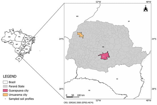
Figure 1. Locations of the sampled soil profiles in Paraná State, southern Brazil (central-southern and northwestern regions).

Table 1. The soil profiles were sampled and classified according to the Brazilian Soil Classification System (SiBCS).

1 SiBCS Soil Class	2 Profile ID	N° of Horizons	3 n
Organossolo Fólico Hêmico Típico	Ooy	2	800
Latossolo Vermelho Tb Distrófico Típico	LVd	3	800
Latossolo Vermelho Distrófico Típico	LVd1	4	800
Latossolo Vermelho Distrófico Típico	LVd2	5	800
Argissolo Vermelho-Amarelo Distrófico Típico	PVAd	3	800
Argissolo Vermelho Distrófico Típico	PVd	5	800

¹ SiBCS, Brazilian Soil Classification System; ² Profile ID, identifier used in this study; ³ n, number of spectral measurements acquired per soil monolith (per sensor). Note: “Profile ID” denotes the identifier used in this study for each monolith, where multiple monoliths belong to the same SiBCS class and numeric suffixes indicate distinct sampled profiles/sites rather than additional SiBCS taxonomic levels.

The use of intact monoliths with high vertical spectral density provides a controlled experimental framework that isolates pedogenic variability from broader landscape heterogeneity, enabling clearer attribution of spectral discrimination to soil-forming processes.

Within each profile, soil samples were collected at 0.10 m depth increments for physical and chemical characterisation. The particle size distribution (sand, silt, and clay) was determined via combined sieving and pipette methods after dispersion with 0.1 mol L⁻¹ NaOH. The soil organic carbon (SOC) content was measured via the Walkley–Black wet oxidation method.

2.2. Spectral Data Acquisition and Pre-Processing

Spectral reflectance measurements were acquired directly on the monolith face, totalling 800 spectra per monolith for each sensor (i.e., 4800 spectra per sensor across the six monoliths; Figure 2). VIS–NIR–SWIR spectra (350–2500 nm) were collected via a FieldSpec 3 Jr spectroradiometer (Analytical Spectral Devices Inc., Boulder, CO, USA) fitted with a contact probe (Analytical Spectral Devices Inc., Boulder, CO, USA), which acquires spectra through direct contact with the soil surface via an internal illumination source. Instrument calibration was performed via a Spectralon diffuse reflectance standard (Labsphere Inc., North Sutton, NH, USA). To avoid re-sampling the same material, the contact probe was repositioned between acquisitions so that the probe footprint did not overlap with previously measured spots; thus, the 800 contact-probe spectra collected per monolith corresponded to 800 distinct measurement locations.

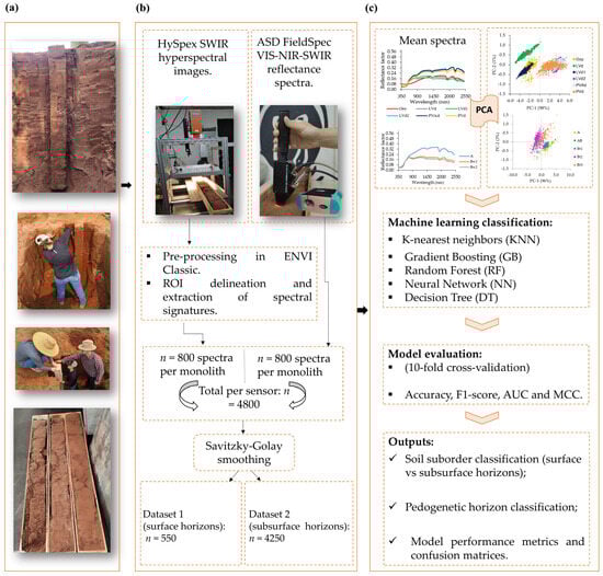
Figure 2. Workflow of the study: (a) collection of soil monoliths; (b) SWIR hyperspectral imaging (HySpex) and VIS–NIR–SWIR spectral acquisition (ASD FieldSpec), including pre-processing and dataset organisation; (c) exploratory analysis (mean spectra and PCA) and machine learning classification with model evaluation.

The spectra were processed in ViewSpec Pro version 6.2 (Analytical Spectral Devices Inc., Boulder, CO, USA) and converted to reflectance via the ratio between the radiance measured on the soil and the radiance measured on the Lambertian reference panel.

$$\rho \left(\lambda \right) ={\displaystyle \frac{L_{\mathrm{soil}}\left(\lambda \right)}{L_{\mathrm{ref}}\left(\lambda \right)}}$$

(1)

where $\rho \left(\lambda \right)$ is the reflectance at wavelength $\lambda$, $L_{\mathrm{soil}}\left(\lambda \right)$ is the radiance recorded on the soil surface, and $L_{\mathrm{ref}}\left(\lambda \right)$ is the radiance recorded on the white reference.

Each monolith was also scanned individually to acquire SWIR hyperspectral images via a HySpex Mjolnir S-620 SWIR camera (Norsk Elektro Optikk AS, Skedsmokorset, Norway; 970–2500 nm), which was mounted on a fixed support above a translation platform. The acquisition speed was set according to the camera frame specifications. The sensor-to-sample distance was fixed at 85 cm to standardise spatial sampling and minimise geometry-driven variability. Acquisition was performed under controlled laboratory conditions: twelve 20 W halogen lamps were evenly placed around the scan window to provide uniform illumination, the ambient temperature was maintained at 25 °C, and external light interference was eliminated. Camera cooling was enabled, and the system was allowed to thermally stabilise prior to acquisition to reduce drift and electronic noise. Reflectance calibration relied on diffuse Spectralon^® (Labsphere Inc., North Sutton, NH, USA) reference target and dark-current measurements, enabling conversion from raw intensity to relative reflectance values.

Image processing was carried out in ENVI Classic version 5.3 (Exelis Visual Information Solutions Inc., Boulder, CO, USA), and the reflectance was obtained via the “Scan Normalisation” procedure. From each reflectance cube, 50 regions of interest were defined at each 0.10 m depth interval via the ENVI ROI tool version 5.3 (Exelis Visual Information Solutions Inc., Boulder, CO, USA), yielding 800 ROI-derived spectra per monolith. ROIs were selected in visually homogeneous areas within each depth interval, avoiding cracks, roots, stones, shadowed pixels and specular highlights. Each ROI comprised a fixed 10 × 5-pixel window (the mean spectrum was extracted per ROI); the ROIs were non-overlapping within monoliths. Noisy portions of the SWIR spectra at the beginning and end of the wavelength range were excluded; therefore, the SWIR interval used in subsequent analyses ranged from 1200–2450 nm. The spectra from both sensors were smoothed via a Savitzky–Golay filter in The Unscrambler X version 10.4 (CAMO Software AS, Oslo, Norway).

2.3. Exploratory Analysis of Spectral Data

Principal component analysis (PCA) was used as an unsupervised approach to summarise spectral variability, visualise sample clustering, and screen for spectra with atypical behaviour prior to supervised modelling. PCA was carried out in The Unscrambler X version 10.4 (CAMO Software AS, Oslo, Norway) using the smoothed reflectance matrices described in Section 2.2. Separate PCA models were fitted to (i) the SWIR spectra and (ii) VIS–NIR–SWIR spectra, each of which was evaluated for surface-horizon and subsurface-horizon datasets. Additional PCA score plots were generated to assess the separation of pedogenetic horizons within each profile.

Potential outliers were assessed via Hotelling’s T² statistic (95%), with observations flagged at p ≤ 0.05 and examined in the score space. Clustering patterns among soil suborders and among horizons were evaluated from PCA score plots, and class separation was described on the basis of the distribution of scores along PC1 and PC2.

2.4. Validation Design and Independence of Data Splits

Evaluation was performed using 10-fold cross-validation, in which the spectra were randomly partitioned into ten mutually exclusive folds, and each fold served as the test set once the remaining nine folds were used for training. No spectrum was used simultaneously for training and testing within a given iteration. The data were shuffled prior to partitioning.

Because multiple spectra/ROIs originate from the same physical monolith (but each spectrum/ROI corresponds to a distinct, non-overlapping measurement location; Section 2.2), spectrum-level random k-fold cross-validation primarily quantifies within-dataset discrimination and may not fully represent transferability to entirely independent profiles if profile-specific spectral structure is strong. Accordingly, we interpret the k-fold results as internal validation within the six-monolith dataset, and we discuss the need for groupwise (e.g., leave-one-profile-out) or spatially blocked validation when broader datasets are available (see Section 4.3).

When hyperparameter optimisation was applied, it was conducted using only the training data (nested within the evaluation procedure) to avoid information leakage into the held-out data.

2.5. Soil Suborder and Horizon Classification via Machine Learning

Supervised classification was performed to predict (i) soil suborders and (ii) pedogenetic horizons from spectral reflectance. For soil suborder classification, datasets were organised separately for each sensor and split into two subsets according to pedogenetic position. The surface-horizon dataset comprises spectra collected within the uppermost horizon of each profile (or organic surface horizon), totalling n = 550 spectra per sensor, whereas the subsurface-horizon dataset comprises spectra from all remaining horizons, totalling n = 4250 spectra. In both cases, the target variable was the soil suborder (Ooy, LVd, LVd1, LVd2, PVAd, and PVd). For horizon classification, models were trained and evaluated separately within each profile via VIS–NIR–SWIR spectra (n = 800 per profile), with the target classes corresponding to the pedogenetic horizons identified during field description (e.g., A, BA, Bw, Bt, Oo, Od). Neural networks were applied only to horizon classification because they provided the most consistent within-profile performance for this multi-class task (Section 3.7); for suborder discrimination, we restricted the benchmark to KNN and tree-based classifiers, which offered strong performance with lower model complexity and clearer interpretability given the limited number of independent profiles.

All modelling was implemented in Orange Data Mining v3.32.0 (Bioinformatics Laboratory, University of Ljubljana, Ljubljana, Slovenia) following the z-score standardisation of predictors (μ = 0, σ² = 1) via the Preprocess widget. Model evaluation used 10-fold cross-validation within the “Test & Score” widget, with folds of approximately equal size. The evaluated algorithms were k-nearest neighbours (KNN), random forest (RF), decision tree, gradient boosting (GB), and a feed-forward neural network (NN). The hyperparameter settings followed the configuration in Table 2, with ranges indicating the values examined during optimisation and the final settings applied consistently during the cross-validation runs; where available, the replicable training option was enabled to ensure reproducible model fitting.

Table 2. Machine learning models and hyperparameter settings used for soil suborder and horizon classification.

Models	Hyperparameter Settings
k-nearest neighbours (KNN)	Number of neighbours: 5; metric: Euclidean; weight: By Distances.
Random Forest (RF)	Number of trees: 10–100; maximal number of considered features: $\sqrt{features}$ in each analysis; replicable training: Yes; maximum tree depth: 8; stop splitting nodes with maximum instances: 5.
Decision Tree	Pruning: at least 2 instances in leaves, at least 5 instances in internal nodes, maximum depth: 30 to 100; splitting: stop splitting when majority reaches 95% (classification only); binary trees: Yes.
Gradient Boosting	Method: scikit-learn; number of trees: 100; learning rate: 0.05; replicable training: Yes; maximum tree depth: 3; fraction of training instances: 1; stop splitting nodes with maximum instances: 2.
Neural Network	Activation: Logistic Solver: Adam Alpha: 0.01; Replicable training: Yes

Ranges indicate values evaluated during hyperparameter optimisation (if applicable). All the models were trained with standardised predictors (μ = 0, σ² = 1) and evaluated via 10-fold cross-validation.

Model performance was quantified via accuracy, the F-score (F1), the area under the ROC curve (AUC), and the Matthews correlation coefficient (MCC). The overall accuracy was computed as the proportion of correctly classified spectra:

$$\begin{array}{cccc}& \mathrm{Accuracy}={\displaystyle \frac{\sum _{i=1}^K{x}_{ii}}{n}}& & \end{array}$$

(2)

where $x_{ii}$ are the diagonal elements of the confusion matrix for $K$ classes and where $n$ is the total number of observations. The F-score was computed as the harmonic mean of precision and recall:

$$\begin{array}{cccc}& F_1=2\times {\displaystyle \frac{\mathrm{Precision}\times \mathrm{Recall}}{\mathrm{Precision}+\mathrm{Recall}}}& & \end{array}$$

(3)

The AUC was computed for multiclass classification via a one-versus-rest strategy, which is based on the integral of the true-positive rate (TPR) as a function of the false-positive rate (FPR):

$$\begin{array}{cccc}& \mathrm{AUC}={{\displaystyle \int }}_0^1\mathrm{TPR}\left(\mathrm{FPR}\right)\hspace{0.17em}\mathrm{d}\left(\mathrm{FPR}\right)& & \end{array}$$

(4)

The MCC was used as a global measure of classification quality derived from the confusion matrix; for multiclass problems, it was computed via the multiclass formulation implemented in Orange, expressed as follows:

$$\begin{array}{cccc}& \mathrm{MCC}={\displaystyle \frac{c\hspace{0.17em}s-\sum _{k=1}^K{p}_k{t}_k}{\sqrt{(s^2-\sum _{k=1}^K{p}_k^2)(s^2-\sum _{k=1}^K{t}_k^2)}}}& & \end{array}$$

(5)

where $c={\sum }_{k=1}^K{x}_{kk}$ is the trace of the confusion matrix, $s=n$ is the total number of observations, $p_k={\sum }_{j=1}^K{x}_{kj}$ are row sums, and $t_k={\sum }_{i=1}^K{x}_{ik}$ are column sums. Confusion matrices were also inspected for the best-performing models; to facilitate comparisons among classes, the matrices were row-normalised so that each measured class was summed to 100%.

Hyperparameter tuning (where applicable) was performed in Orange (Tune Model) using only the training data within each cross-validation iteration to prevent information leakage. Candidate settings (ranges in Table 2) were compared by internal cross-validation on the training folds, and the configuration maximising the macro-averaged F1-score was selected (with the MCC inspected as a complementary metric). The selected hyperparameters were then fixed for the outer 10-fold cross-validation evaluation.

3. Results

3.1. Soil Properties

Table 3 shows that the sampled profiles spanned a wide textural range, from very clayey horizons dominated by the clay fraction to sand-rich horizons with comparatively low fines. Across all the profiles, the silt contents were generally minor (typically ≤6%), indicating that the particle–size distributions were largely governed by the sand–clay balance.

Table 3. Mean particle size distribution, soil organic carbon (SOC), and moisture colour for each horizon in the sampled soil profiles.

Class	Id	Horizon		Particle-Size Distribution (%)			SOC	Soil Colour When Moist
SiBCS		Symbol	Depth (m)	Sand	Silt	Clay	g dm−3	Hue, Value, Chroma
Organossolo Fólico Hêmico Típico	Ooy	Oo	0.00–0.30	22	3	75	56.0	10YR 2/1
		Od	0.30–1.60	15	5	80	38.9	10YR 2/1
Latossolo Vermelho Tb Distrófico Típico		A	0.00–0.10	7	6	87	44.8	2.5YR 3/2
	LVd	Bw1	0.10–1.00	6	3	91	13.1	2.5YR 3/4
		Bw2	1.00–1.60	13	2	85	4.2	2.5YR 3/4
Latossolo Vermelho Distrófico Típico		A	0.00–0.10	7	4	89	29.7	2.5YR 3/2
		BA	0.10–0.30	5	3	92	26.3	2.5YR 3/2
	LVd1	Bw1	0.30–1.10	6	2	92	17.6	2.5YR 3/4
		Bw2	1.10–1.60	6	2	92	8.6	2.5YR 3/4
Latossolo Vermelho Distrófico Típico		A	0.00–0.20	75	2	23	3.6	10R 3/4
		Bw1	0.20–0.60	75	2	23	1.4	10R 3/6
	LVd2	Bw2	0.60–0.90	78	1	21	1.1	10R 3/4
		Bw3	0.90–1.10	80	1	19	1.1	10R 3/6
		Bw4	1.10–1.60	77	1	22	0.8	10R 3/6
Argissolo Vermelho-Amarelo Distrófico Típico		A	0.00–0.20	81	1	18	6.9	5YR 3/4
	PVAd	Bt1	0.20–0.90	73	2	25	3.6	5YR 3/4
		Bt2	0.90–1.60	76	2	22	2.0	5YR 3/3
Argissolo Vermelho Distrófico Típico		A	0.00–0.20	84	2	14	8.7	10R 3/2
		AB	0.20–0.30	82	1	17	5.5	10R 3/4
	PVd	Bt1	0.30–0.80	78	1	21	2.6	10R 3/4
		Bt2	0.80–1.40	63	2	35	2.4	10R 3/6
		Bt3	1.40–1.60	65	1	34	10.4	10R 3/6

Notes: SOC = soil organic carbon (Walkley–Black). The particle size distribution was determined via the pipette/sieving method. The colour-reference is given in Munsell notation under moist conditions.

The Organossolo Fólico Hêmico Típico (Ooy) combined a very clayey mineral matrix (75–80% clay) with the highest soil organic carbon (SOC) concentrations observed in the dataset, reaching 56.0 g dm⁻³ in the Oo horizon and remaining high at depth (38.9 g dm⁻³ in Od). The moist colour was uniformly very dark (10YR 2/1) throughout the profile, which is consistent with sustained organic matter dominance in the visual expression of the soil matrix.

The two clayey Latossolos (LVd and LVd1) were consistently very clayey across their sampled horizons, with clay contents between 85% and 92% and sand remaining low (5–13%). Both profiles exhibited limited vertical variation in clay content, indicating weak textural differentiation with depth. In these Latossolos, the SOC content sharply decreased: the surface horizons contained relatively high SOC contents (29.7–44.8 g dm⁻³), whereas the deepest Bw horizons contained much lower SOC contents (4.2–8.6 g dm⁻³). The moist colours were persistently red, with darker surface hues (2.5YR 3/2) and slightly brighter subsurface colours (2.5YR 3/4).

In contrast, LVd2 was coarse-textured throughout, with a sand content of 75–80% and a clay content between 19% and 24%. This profile also exhibited uniformly low SOC, from 3.6 g dm⁻³ at the surface to 0.8–1.4 g dm⁻³ in subsurface horizons, alongside intense red moist colours (10R 3/4–3/6).

The Argissolos (PVAd and PVd) samples presented sand-dominated surface horizons and increased clay contents in subsurface Bt horizons, which was consistent with a clear textural contrast within each profile. In the PVAd, the A horizon was sandy loam in texture (81% sand; 18% clay), whereas the Bt horizons were finer (22–25% clay), accompanied by a decrease in the SOC profile from 6.9 to 2.0 g dm⁻³. Moist colour remained within the 5YR hue range, with a slight reduction in chroma in the deeper Bt2 horizon (5YR 3/3). In the PVd, the upper horizons (A–Bt1) remained sand-rich (77–84% sand) with lower clay (14–21%), whereas the deeper Bt horizons reached substantially higher clay contents (33–35%). The SOC decreased from 8.7 g dm⁻³ in the surface horizon to 2.4–2.6 g dm⁻³ in Bt1–Bt2 but increased again in the deepest sampled horizon (10.4 g dm⁻³ in Bt3), which contrasts with the monotonic declines observed in the Latossolos.

3.2. Spectral Behaviour of Soil Horizons and Suborders

The mean VIS–NIR–SWIR spectra (350–2500 nm) revealed marked within-profile contrasts in spectral intensity for some profiles, alongside clear between-soil separation in overall albedo and diagnostic absorptions (Figure 3). Across the dataset, differences among horizons were expressed primarily as changes in spectral intensity (albedo), whereas differences among soil suborders were expressed both in intensity and in the relative prominence of iron- and clay-related spectral features.

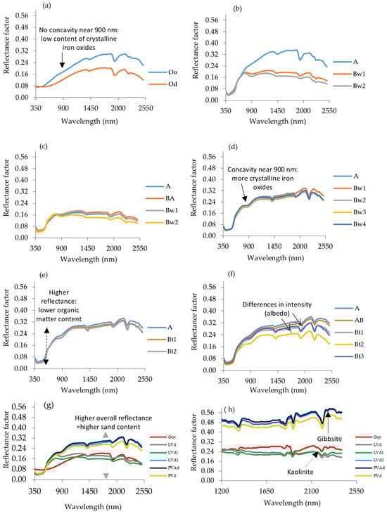
Figure 3. Mean reflectance spectra of the soil horizons and suborders: (a) Ooy; (b) LVd; (c) LVd1; (d) LVd2; (e) PVAd; (f) PVd; (g) mean VIS–NIR–SWIR spectra (350–2500 nm) by soil suborder; and (h) mean SWIR spectra (1200–2450 nm) by soil suborder. Curves represent the mean reflectance; within-horizon variability is explored via PCA (Figures 4 and 5, see below) and is reflected in the class overlap and confusion patterns in the classification results (Tables 4–6; Figures 6–8, see below).

In Organossolo (Ooy) and clayey Latossolo (LVd), the surface horizons displayed higher reflectances than their subsurface counterparts did (Figure 3a,b). In Ooy, the Oo horizon maintained a consistently higher reflectance than Od throughout the spectrum, and both horizons lacked a pronounced concavity at ~900 nm (Figure 3a), indicating weak expression of crystalline iron oxide absorption within the sampled material. In LVd, the A horizon presented the highest reflectance, whereas the Bw horizons presented a systematically lower curve (Figure 3b). The subsurface LVd horizons also exhibited a clearer inflection at ~900 nm than did the surface horizon, which was consistent with the stronger spectral expression of crystalline Fe oxides at depth, whereas the surface signal appeared to be relatively muted in that region.

The second clayey Latossolo (LVd1) showed minimal spectral stratification: curves from the A, BA and Bw horizons largely overlapped across VIS–NIR–SWIR wavelengths (Figure 3c), indicating that the vertical variability captured by spectroscopy was small relative to the between-profile variability. In contrast, the sandier Latossolo (LVd2) exhibited a distinctly higher overall reflectance and a more evident concavity at ~900 nm across its horizons (Figure 3d). This combination of high albedo with a strong ~900 nm feature points to a spectrum dominated by efficient scattering from a quartz-rich matrix while still retaining a conspicuous absorption associated with more crystalline iron phases.

The two Argissolos (PVAd and PVd) showed broadly similar spectral shapes, with differences expressed mainly in albedo rather than in the position of absorption features (Figure 3e,f). In PVAd, the A, Bt1 and Bt2 horizons followed closely aligned trajectories, with consistently high reflectances throughout the VIS–NIR–SWIR domain (Figure 3e). In PVd, the spectral intensity varied more strongly among horizons (Figure 3f): the clay-enriched Bt horizons, particularly Bt2 and Bt3, as indicated by the particle-size distribution (Table 3), exhibited lower reflectances than the sandier upper horizons did, reflecting stronger net absorption and reduced multiple scattering typically associated with finer-textured, more pigment-rich subsurface material.

When the spectra were aggregated by soil suborder, two spectral “families” became apparent (Figure 3g). The clay-rich soils (Ooy, LVd and LVd1) clustered at lower reflectances, whereas the sand-rich profiles (LVd2, PVAd and PVd) clustered at higher reflectances, with the greatest separation occurring in the NIR and SWIR regions, where mineralogical and textural controls on scattering dominate. The ~900 nm feature, which is indicative of iron oxide absorption, was most evident in the spectra with higher overall intensity (Figure 3g), where high albedo makes concavity easier to resolve. In the SWIR window (1200–2450 nm), absorption features centred near ~2200 nm and ~2260 nm were evident in the mean spectra (Figure 3h), which is consistent with the Al–OH combination bands typically attributed to kaolinite (~2200 nm) and gibbsite (~2260 nm). The clearer expression of these clay–mineral features in the higher-albedo spectra indicates that, beyond composition, the background scattering environment modulates how strongly mineralogical signatures are expressed in reflectance space.

3.3. Principal Component Analysis of the Soil Suborders

Figure 4 presents PCA score plots derived from spectral reflectance data for the sampled soil suborders, considering the SWIR-only and full VIS–NIR–SWIR inputs and separating the surface and subsurface horizons. In all the cases, PC1 accounted for the dominant share of variance, explaining 97% (SWIR surface; Figure 4a), 91% (VIS–NIR–SWIR surface; Figure 4b), 98% (SWIR subsurface; Figure 4c), and 92% (VIS–NIR–SWIR subsurface; Figure 4d) of the variance. PC2 explained a smaller fraction of the variance, corresponding to 2%, 5%, 1%, and 6% for panels (a–d), respectively.

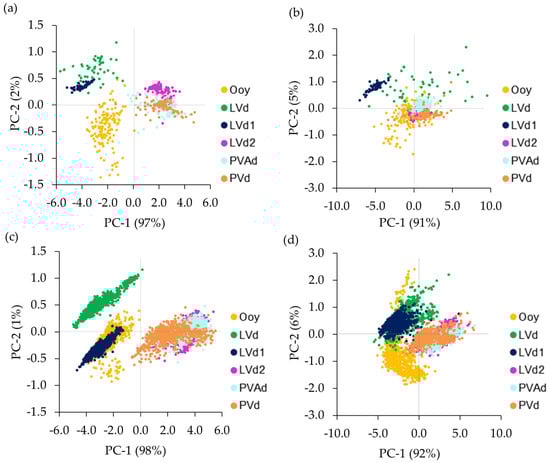
Figure 4. Principal component analysis (PCA) score plots for soil suborders via spectral reflectance data: (a) SWIR surface horizons; (b) VIS–NIR–SWIR surface horizons; (c) SWIR subsurface horizons; and (d) VIS–NIR–SWIR subsurface horizons. The percentages indicate the variance explained by each principal component.

Using the SWIR reflectance from the surface horizons (Figure 4a), LVd2, PVAd and PVd formed a compact group at positive PC1 scores, whereas Ooy, LVd and LVd1 were positioned at negative PC1 scores. Within the negative PC1 domain, compared with the other classes, LVd was associated with predominantly positive PC2 scores, whereas Ooy tended toward negative PC2 scores, and LVd1 was concentrated at more negative PC1 values.

When the surface-horizon PCA was performed using the full VIS–NIR–SWIR range (Figure 4b), the separation among classes was less distinct, with increased overlap in score space. LVd showed the broadest dispersion across both PC1 and PC2. LVd2, PVAd and PVd remained concentrated near the central to positive portion of PC1, although their clusters overlapped more strongly than in the SWIR-only PCA did. LVd1 retained a distinct position at negative PC1 values with positive PC2 values.

For subsurface horizons analysed via SWIR reflectance (Figure 4c), class separation was pronounced along PC1, with LVd2, PVAd and PVd located at positive PC1 scores and Ooy, LVd and LVd1 located at negative PC1 scores. LVd also showed a marked displacement toward higher PC2 scores relative to the other classes, whereas LVd1 was concentrated at negative PC1 with slightly negative to near-zero PC2 values.

In the VIS–NIR–SWIR PCA of subsurface horizons (Figure 4d), LVd2 and PVAd were grouped at positive PC1 scores, and PVd occupied an intermediate position, extending from near-zero to positive PC1 values. Ooy, LVd and LVd1 were mainly distributed at negative PC1 scores, with Ooy spanning a relatively wide range of PC2 values and LVd concentrated at positive PC2 values.

3.4. Principal Component Analysis of Pedogenetic Horizons

Figure 5 shows PCA score plots constructed from VIS–NIR–SWIR reflectance (350–2500 nm) for horizons within each soil profile. In Ooy, PC1 and PC2 explained 85% and 13% of the variance, respectively (Figure 5a), and the two horizons clearly formed separate score domains. Oo was concentrated at positive PC1 scores, whereas Od occupied predominantly negative PC1 scores and displayed a wider spread along PC2.

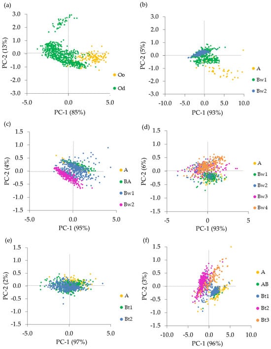
Figure 5. PCA score plots for pedogenetic horizons within each soil profile via VIS–NIR–SWIR reflectance spectra (350–2500 nm): (a) Ooy; (b) LVd; (c) LVd1; (d) LVd2; (e) PVAd; and (f) PVd.

In LVd, PC1 explained 93% of the variance, and PC2 explained 5% (Figure 5b). The Bw1 and Bw2 scores overlapped strongly and clustered around the centre of the plot, whereas the A horizon formed a separate distribution displaced towards positive PC1 and negative PC2.

In LVd1, PC1 and PC2 accounted for 95% and 4% of the variance, respectively (Figure 5c). The A, BA and Bw1 horizons showed substantial overlap in score space, whereas Bw2 formed a distinct cluster that shifted towards more negative PC2 values relative to the other horizons.

In LVd2, PC1 explained 93% of the variance, and PC2 explained 6% (Figure 5d). The scores from all horizons overlapped broadly, with Bw1 forming a compact cluster near the origin and slightly negative PC2 values, whereas A and the remaining Bw horizons were predominantly distributed at neutral to positive PC2 values with similar PC1 scores.

In the PVAd, PC1 and PC2 explained 97% and 2% of the variance, respectively (Figure 5e). The A, Bt1 and Bt2 horizons strongly overlap, with scores concentrated close to the origin and only minor dispersion along PC2.

For PVd, PC1 explained 96% of the variance, and PC2 explained 3% (Figure 5f). The A and AB horizons showed substantial overlap at positive PC1 values, Bt1 clustered near the plot centre, and Bt2 was concentrated at negative PC1 scores. Bt3 overlapped partially with Bt2 towards negative to near-zero PC1 values but extended to higher PC2 scores.

3.5. Machine Learning Classification of Soil Suborders via Surface-Horizon Spectra

Table 4 summarises the performance of the machine learning models for soil-suborder classification via surface-horizon spectra. Using the SWIR reflectance, the overall accuracy ranged from 0.83–0.89. The k-nearest neighbour model achieved the highest accuracy (0.89) and F-score (0.89), followed by gradient boosting (accuracy = 0.88; F-score = 0.88) and random forest (accuracy = 0.87; F-score = 0.87). These three models had identical AUC values (0.98), with MCC values of 0.87 (k-nearest neighbours), 0.85 (gradient boosting) and 0.83 (random forest). The decision tree model showed the lowest performance with the SWIR data (accuracy = 0.83; AUC = 0.90; MCC = 0.79).

Table 4. Performance of machine learning models for soil suborder classification via surface-horizon spectra.

Model	SWIR				VIS–NIR–SWIR
	Accuracy	F-Score	AUC	MCC	Accuracy	F-Score	AUC	MCC
K-Nearest Neighbours	0.89	0.89	0.98	0.87	0.86	0.85	0.94	0.82
Random Forest	0.87	0.87	0.98	0.83	0.79	0.78	0.94	0.74
Decision Tree	0.83	0.83	0.90	0.79	0.76	0.76	0.87	0.71
Gradient Boosting	0.88	0.88	0.98	0.85	0.79	0.80	0.94	0.75

Note: SWIR spectra were derived from a hyperspectral imaging sensor (HySpex; analysis range 1200–2450 nm). VIS–NIR–SWIR spectra were derived from a non-imaging spectroradiometer (FieldSpec; 350–2500 nm). Metrics were computed via 10-fold cross-validation. AUC = area under the ROC curve (multiclass, one-versus-rest). MCC = Matthews correlation coefficient.

With VIS–NIR–SWIR reflectance, the highest accuracy was again obtained with k-nearest neighbours (0.86), whereas the accuracy of random forest and gradient boosting reached 0.79, and that of the decision tree reached 0.76. The F-scores followed the same pattern, with values of 0.85 (k-nearest neighbours), 0.78 (random forest), 0.80 (gradient boosting) and 0.76 (decision tree). The AUC values were 0.94 for k-nearest neighbours, random forest and gradient boosting, and 0.87 for the decision tree; the MCC values ranged from 0.71 (decision tree) to 0.82 (k-nearest neighbours).

Figure 6 shows the row-normalised confusion matrices for the three best-performing models (k-nearest neighbours, random forest and gradient boosting) using the SWIR and VIS–NIR–SWIR surface-horizon spectra. For the SWIR inputs (Figure 6a,c,e), the highest diagonal values were observed for Ooy (97.0–98.0), LVd1 (94.0–100.0), LVd2 (88.0–90.0) and PVd (82.1–87.0), whereas PVAd (75.0–80.0) and LVd (74.0–84.0) presented lower diagonal values. The greatest off-diagonal contributions for the SWIR band were concentrated between PVAd and PVd and between LVd2 and PVAd. In the random forest model, 16.0% of the PVd samples were predicted as PVAd, whereas 16.0% of the PVAd samples were predicted as PVd (Figure 6c). Across the three SWIR-based models, PVAd was predicted as LVd2 in 7.0–9.0% of the cases, and LVd2 was predicted as PVAd in 8.0–11.0% of the cases (Figure 6a,c,e).

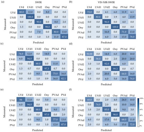
Figure 6. Row-normalised confusion matrices (%) for soil suborder classification via surface-horizon spectra: (a,b) k-nearest neighbours (KNN); (c,d) random forest; (e,f) gradient boosting. (Left panels): SWIR; (right panels): VIS–NIR–SWIR. The values are normalised to 100% within each measured class (rows). The main confusion occurred between PVAd and PVd and between LVd2 and PVAd, which is consistent with their similar albedo-dominated spectral behaviour.

With respect to the VIS–NIR–SWIR inputs (Figure 6b,d,f), the diagonal values remained high for Ooy (98.0–100.0) and LVd2 (85.0–96.0), whereas LVd ranged from 50.0–72.0 and LVd1 ranged from 58.0–80.0. The lowest diagonal values were again associated with PVAd (64.0–71.0) and PVd (72.0–78.0). The off-diagonal contributions were distributed across multiple classes: LVd was predicted as PVAd in 11.9–24.0% of the cases and as PVd in 6.1–10.0% of the cases; PVAd was predicted as LVd2 in 16.0–20.0% of the cases; and PVAd and PVd showed reciprocal confusion (PVAd→PVd: 11.0–14.0%; PVd→PVAd: 13.0–15.0%) (Figure 6b,d,f).

3.6. Machine Learning Classification of Soil Suborders Using Subsurface-Horizon Spectra

Table 5 reports the cross-validated performance of the four models trained with subsurface-horizon spectra. Using the SWIR reflectance, the overall accuracy ranged from 0.89–0.96. Gradient boosting yielded the highest values across all the metrics (accuracy = 0.96; F-score = 0.96; AUC = 0.99; MCC = 0.95). The k-nearest neighbours also showed high performance (accuracy = 0.94; F-score = 0.94; AUC = 0.99; MCC = 0.93), followed by the random forest (accuracy = 0.90; F-score = 0.90; AUC = 0.98; MCC = 0.88) and decision tree (accuracy = 0.89; F-score = 0.89; AUC = 0.94; MCC = 0.87) classifiers.

Table 5. Performance of machine learning models for soil suborder classification via subsurface-horizon spectra.

Model	SWIR				VIS-NIR-SWIR
	Accuracy	F-Score	1 AUC	2 MCC	Accuracy	F-Score	1 AUC	2 MCC
K-Nearest Neighbours	0.94	0.94	0.99	0.93	0.87	0.87	0.97	0.84
Random Forest	0.90	0.90	0.98	0.88	0.82	0.82	0.97	0.78
Decision Tree	0.89	0.89	0.94	0.87	0.81	0.80	0.88	0.77
Gradient Boosting	0.96	0.96	0.99	0.95	0.85	0.85	0.98	0.82

Note: SWIR spectra were derived from a hyperspectral imaging sensor (HySpex; analysis range 1200–2450 nm). VIS–NIR–SWIR spectra were derived from a non-imaging spectroradiometer (FieldSpec; 350–2500 nm). Metrics were computed via 10-fold cross-validation. ¹ AUC = area under the ROC curve (multiclass, one-versus-rest). ² MCC = Matthews correlation coefficient.

When VIS–NIR–SWIR reflectance was used, the accuracy values ranged from 0.81–0.87. The k-nearest neighbours achieved the highest accuracy and F-scores (0.87 and 0.87) with AUC = 0.97 and MCC = 0.84. Gradient boosting reached an accuracy of 0.85 (F-score = 0.85; AUC = 0.98; MCC = 0.82), random forest reached 0.82 (F-score = 0.82; AUC = 0.97; MCC = 0.78), and the decision tree reached 0.81 (F-score = 0.80; AUC = 0.88; MCC = 0.77).

Figure 7 presents row-normalised confusion matrices for the three best-performing models (k-nearest neighbours, random forest and gradient boosting) using the SWIR and VIS–NIR–SWIR subsurface-horizon spectra. For the SWIR inputs (Figure 7a,c,e), the diagonal values were the highest for LVd (99.7–100.0), LVd1 (99.4–99.8) and Ooy (98.5–99.3). PVd also had high diagonal values (84.9–92.9), whereas LVd2 (80.7–93.0) and PVAd (79.2–91.9) presented lower diagonal values and greater cross-confusion. In the random forest model, LVd2 was predicted as PVAd in 17.4% of the cases and as PVd in 2.0% of the cases (Figure 7c), whereas PVAd was predicted as LVd2 in 17.2% of the cases and as PVd in 3.6% of the cases. The gradient boosting model showed reduced cross-confusion between LVd2 and PVAd, with LVd2 being predicted as PVAd in 5.4% of the cases and as PVd in 1.6% of the cases (Figure 7e).

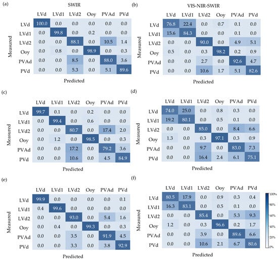
Figure 7. Row-normalised confusion matrices (%) for soil suborder classification via subsurface-horizon spectra: (a,b) k-nearest neighbours (KNN); (c,d) random forest; (e,f) gradient boosting. (Left panels): SWIR; (right panels): VIS–NIR–SWIR. The values are normalised to 100% within each measured class (rows). The main confusion occurred between PVAd and PVd and between LVd2 and PVAd, which is consistent with their similar albedo-dominated spectral behaviour.

For VIS–NIR–SWIR inputs (Figure 7b,d,f), the diagonal values remained high for Ooy (96.6–98.2), whereas LVd and LVd1 presented lower diagonals and stronger reciprocal mixing. Across the three models, LVd samples were predicted as LVd in 74.0–80.5% of the cases and as LVd1 in 17.9–24.9% of the cases, whereas LVd1 samples were predicted as LVd1 in 80.1–84.3% of the cases and as LVd in 15.6–19.2% of the cases (Figure 7b,d,f). LVd2 retained diagonal values between 85.0% and 90.0%, with the main off-diagonal contributions coming from PVAd (4.9–8.4%) and PVd (5.1–9.3%). For PVAd and PVd, the diagonal values ranged from 83.0% to 92.6% (PVAd) and from 75.1% to 82.6% (PVd), respectively, with off-diagonal contributions primarily involving LVd2 and reciprocal confusion between PVAd and PVd (PVAd→PVd: 4.7–7.3%; PVd→PVAd: 5.1–6.7%) (Figure 7b,d,f).

3.7. Horizon Classification via Machine Learning Models and VIS–NIR–SWIR Reflectance Spectra

Table 6 summarises the within-profile classification performance for pedogenetic horizons via VIS–NIR–SWIR spectra. Across the six profiles, the neural network achieved accuracies between 0.84 and 0.97, with F-scores between 0.84 and 0.97 and AUC values between 0.94 and 0.99. The highest neural network accuracy was obtained for LVd1 (0.97), and the lowest was obtained for LVd2 (0.84), while Ooy, LVd, PVAd and PVd achieved accuracies of 0.96, 0.88, 0.86 and 0.90, respectively. The random forest accuracies ranged from 0.73 (PVAd) to 0.95 (Ooy), with AUC values ranging from 0.85 to 0.99. The gradient boosting accuracies ranged from 0.74 (PVAd) to 0.97 (PVd), with AUC values ranging from 0.85 to 0.99. The k-nearest neighbour model yielded accuracies between 0.72 (PVAd) and 0.96 (Ooy), with AUC values ranging from 0.83 to 0.98.

Table 6. Performance of machine learning models for pedogenetic horizon classification within each soil profile (VIS–NIR–SWIR).

Model	Metric	Soil Class
		Ooy	LVd	LVd1	LVd2	PVAd	PVd
Neural Network	Accuracy	0.96	0.88	0.97	0.84	0.86	0.90
	F-Score	0.95	0.88	0.97	0.84	0.86	0.90
	AUC	0.98	0.95	0.99	0.97	0.94	0.98
Random Forest	Accuracy	0.95	0.78	0.92	0.78	0.73	0.80
	F-Score	0.96	0.77	0.92	0.78	0.72	0.80
	AUC	0.97	0.88	0.99	0.95	0.85	0.94
Gradient Boosting	Accuracy	0.96	0.81	0.91	0.77	0.74	0.97
	F-Score	0.96	0.81	0.91	0.77	0.74	0.95
	AUC	0.98	0.90	0.98	0.94	0.85	0.99
K-Nearest Neighbours	Accuracy	0.96	0.78	0.92	0.77	0.72	0.86
	F-Score	0.96	0.78	0.92	0.77	0.72	0.86
	AUC	0.97	0.87	0.98	0.93	0.83	0.96

Note: Metrics refer to horizon classification performed separately within each profile via VIS–NIR–SWIR spectra. AUC = area under the ROC curve (multiclass, one-versus-rest).

The row-normalised confusion matrices for the neural network model are shown in Figure 8, indicating the distribution of the predicted horizons within each measured horizon class. For LVd2 (Figure 8a), the diagonal values were 95.0% for A, 88.5% for Bw1, 69.3% for Bw2, 74.0% for Bw3 and 90.4% for Bw4. Most confusion occurred among the Bw horizons: Bw2 was predicted as Bw1 in 22.7% of the cases and as Bw3 in 8.0% of the cases, Bw1 was predicted as Bw2 in 8.0% of the cases, and Bw3 was predicted as Bw4 in 17.0% of the cases (Figure 8a). For PVd (Figure 8b), the diagonal values were 88.0% for A, 60.0% for AB, 89.0% for Bt1, 93.0% for Bt2 and 92.0% for Bt3; the main off-diagonal contribution was the reciprocal confusion between A and AB (A→AB: 4.0%; AB→A: 32.0%), and AB was also predicted as Bt1 in 8.0% of the cases (Figure 8b). For LVd1 (Figure 8c), the diagonal values were 92.0% for A, 93.0% for BA, 98.0% for Bw1 and 98.8% for Bw2, with most misclassifications occurring between A and BA (A→BA: 8.0%; BA→A: 6.0%) and minor confusion between Bw1 and Bw2 (Bw1→Bw2: 1.7%; Bw2→Bw1: 1.2%). In the PVAd (Figure 8d), Bt1 and Bt2 showed reciprocal confusion (Bt1→Bt2: 17.4%; Bt2→Bt1: 11.7%), whereas A remained well classified (90.0%). In LVd (Figure 8e), the diagonal values were 78.0% for A, 91.3% for Bw1 and 83.7% for Bw2, with the main confusion between Bw1 and Bw2 (Bw1→Bw2: 8.4%; Bw2→Bw1: 16.0%). For Ooy (Figure 8f), the diagonal values were 90.0% for Oo and 97.1% for Od, with Oo predicted as Od in 10.0% of the cases and Od predicted as Oo in 2.9% of the cases.

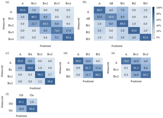
Figure 8. Row-normalised confusion matrices (%) for pedogenetic horizon classification via the neural network model: (a) LVd2; (b) PVd; (c) LVd1; (d) PVAd; (e) LVd; and (f) Ooy. The values are normalised to 100% within each measured horizon class (rows). Most misclassifications occurred between vertically adjacent horizons (e.g., Bw2–Bw3–Bw4 in LVd2; A–AB and Bt1–Bt2 in PVd; Bt1–Bt2 in PVAd), which is consistent with gradual spectral transitions along the profile.

4. Discussion

4.1. Pedogenic Controls on Spectral Expression Across Profiles and Horizons

The spectral behaviour observed across the six profiles is consistent with competition between strongly absorbing phases (organic matter, iron oxides and hydroxyl-bearing clay minerals) and highly scattered phases dominated by quartz-rich fractions [24,25,26,27,28]. In the clay-rich profiles, the progressive strengthening of the diagnostic absorption structure in the VIS–NIR bands (notably around the broad Fe-related feature in the 800–1000 nm region) suggests that subsurface materials increasingly express iron–oxide signatures once the surface-specific masking effects are reduced [29,30,31,32,33,34,35]. Laboratory experiments have demonstrated that organic matter can attenuate and even obliterate iron oxide absorption features in the VIS–NIR region, with the masking threshold depending on organic matter type and concentration [35,36,37]; this provides a mechanistic framework for understanding why near-surface spectra may retain higher albedo or weaker Fe-driven concavity even when soils are otherwise iron rich [24,38,39,40,41,42].

In the quartz-rich profiles, the higher and more uniform albedo across VIS–NIR–SWIR indicates a radiative-transfer regime dominated by multiple scattering from coarse mineral grains, which reduces the contrast of mineral-specific absorptions and compresses interclass separability in spectral space [40]. This is particularly relevant when distinct taxonomic units share a common lithological template because the parent material control on quartz abundance can overwhelm subtler spectral differences associated with horizonation and clay translocation. Depth-resolved spectroscopy has previously shown that spectral–texture relationships and their predictive stability can vary substantially with the depth interval considered, highlighting the importance of explicitly separating surface and subsurface layers when the aim is classification rather than property prediction [25].

The SWIR domain remains critical because it contains overtone and combination bands linked to hydroxyl groups in secondary minerals, providing a mineralogical “process fingerprint” of weathering intensity. The absorption structures at ~2200 nm and ~2260 nm are consistent with kaolinite- and gibbsite-related vibrations [23,29], and the relative prominence of these features can be interpreted as a proxy for the balance between silicate weathering, desilication, and aluminium-hydroxide accumulation. Recent work in Brazilian soils has explicitly used Vis–NIR–SWIR diffuse reflectance to map kaolinite–gibbsite relationships at the landscape scale, supporting the interpretation that these SWIR features encode pedogenic differences that should be detectable even when grain-size effects inflate albedo [1,26,43,44].

A testable hypothesis that emerges from the combined horizon and suborder patterns is that, in clay-rich Ferralsol/Latosol materials, the depth-dependent increase in Fe-oxide spectral expression reflects not only a decrease in surface masking but also an aging trajectory in which iron oxides become more crystalline with increasing depth as organic ligands, redox oscillations, and bioturbation diminish. This mechanism could be evaluated by pairing continuum-removed Fe feature indices with selective dissolution metrics (e.g., oxalate- vs dithionite-extractable Fe) and mineralogical quantification, thereby linking spectral changes to explicit pedogenic kinetics rather than treating them as purely statistical correlates [21,27,41,43].

4.2. PCA as an Exploratory Decomposition of Functional Spectral Variability

The PCA results indicate that a single dominant axis captured most of the spectral variability among the soil suborders, implying that a broad compositional contrast—rather than many independent, small-amplitude effects—structures the spectral space. Given the clustering patterns, this dominant axis is most plausibly associated with the integrated albedo–absorption balance driven by quartz scattering versus clay/oxide/organic absorption, which is consistent with the strong separation between quartz-rich and clay-rich groups in the SWIR-based ordinations [38,42,43,44,45,46,47]. Importantly, the greater overlap observed when the VIS–NIR region was included suggests that adding wavelengths can increase within-class variance when those wavelengths are sensitive to transient surface controls (microroughness, organic coatings, moisture gradients, and illumination–contact effects), thereby weakening group separability despite the larger feature set. Similarly, evidence from multirange soil classification studies indicates that expanding or fusing spectral domains does not guarantee improved discrimination and can even dilute diagnostically strong ranges when additional domains introduce redundancy or noise [6,38,42,43,44,45,46].

Although the second component explained a small fraction of the variance, its capacity to separate specific suborders and horizons implies that it may encode mechanistically meaningful, process-linked variation that is orthogonal to the dominant albedo gradient [48,49,50]. A productive next step is to investigate PCA loadings (and/or continuum-removed band–depth ratios) to identify whether PC2 aligns with Fe-oxide crystallinity proxies in the VIS–NIR or with kaolinite–gibbsite contrast in the SWIR. This would convert PCA from a purely visual clustering tool into a hypothesis generator for pedogenic thresholds, for example, by testing whether the wavelengths driving PC2 correspond to mineral assemblage transitions expected under differing weathering regimes or parent materials [21,27,28,29].

4.3. Why Subsurface SWIR Improved Suborder Discrimination via Machine Learning

The consistently stronger classification performance achieved with subsurface spectra is mechanistically consistent with the idea that subsurface horizons preserve more stable mineralogical and textural signals, whereas surface horizons amplify transient and anthropogenically mediated variability. In many settings, surface layers exhibit greater spatial heterogeneity in terms of organic inputs, aggregation, and moisture dynamics, all of which alter scattering and mask diagnostic mineral absorption; subsurface layers, in contrast, better reflect longer-term pedogenic processes such as clay translocation, oxide accumulation and mineral transformation. Depth-resolved taxonomic prediction has previously demonstrated improved discrimination when focusing on diagnostically informative subsurface layers (often B horizons), reinforcing the inference that subsurface spectra better encode taxonomic signals than surface spectra alone do [30,45,46,47,48,49].

The stronger performance of the SWIR-only data, relative to the full VIS–NIR–SWIR range, suggests that mineralogical absorptions in the SWIR provided a more robust decision basis than VIS-driven colour and chromophore effects in this dataset [31]. This aligns with broader soil classification evidence that, depending on the classes involved, adding weaker or more disturbance-sensitive spectral regions can degrade discrimination by increasing collinearity and introducing variability unrelated to the targeted pedogenic differences [2,21]. A recent global-scale classification comparison, for example, reported that fusing vis–NIR with MIR did not necessarily outperform the best single-range models, underscoring that “more wavelengths” are not synonymous with “more separable classes” [9,32].

From a pedological perspective, the remaining confusion among quartz-rich classes indicates that spectral similarity can reflect genuine convergence in mineralogy and texture driven by shared parent material, even when taxonomic separation depends on diagnostic horizon criteria that are only weakly expressed in reflectance. This points to an important boundary condition for spectroscopy-only classification: where the dominant control is a high-quartz matrix, additional sources of information that directly capture pedogenic redistribution (e.g., MIR fundamentals, pXRF elemental ratios, or structural descriptors from imaging texture) may be required to resolve classes that are pedogenetically distinct yet spectrally convergent in the VIS–NIR–SWIR [27,30].

A second boundary condition concerns generalisation. Because each monolith contributes many spectra from distinct sampling locations, random spectrum-level k-fold cross-validation can still inflate the apparent performance if spectra from the same monolith are split between training and testing, allowing the model to leverage profile-specific spectral idiosyncrasies. Spatially explicit or groupwise validation (e.g., leave-one-profile-out, blocking by depth intervals, or region-wise holdout) would provide a more stringent estimate of transfer across landscapes and is increasingly considered essential for honest assessment of geospatial prediction [33].

A mechanistic route to improve transfer is to treat soil spectroscopy as a domain-shift problem: the spectra–class relationship learned in one landscape may not hold in another because the conditional distributions differ with mineralogy, moisture regime, and measurement geometry. Transfer-learning approaches designed for soil spectral libraries explicitly target this issue by borrowing information from large libraries while fitting local calibration points; adopting such approaches for taxonomic classification, combined with uncertainty-aware decision rules, would allow models to signal when a sample lies outside the training domain rather than forcing overconfident class assignments [34,35].

Importantly, the present dataset was designed to evaluate controlled vertical spectral structure within representative profiles rather than to maximise geographic heterogeneity (Figure 3, Figure 4, Figure 5, Figure 6, Figure 7 and Figure 8 and Table 3, Table 4 and Table 5). Accordingly, the strong discrimination observed here reflects consistent pedogenic spectral patterns under controlled conditions and should be viewed as evidence of mechanistic separability rather than immediate large-scale transferability.

4.4. Horizon Classification and the Spectral Continuity of Profile Development

Within-profile horizon classification highlights a fundamental feature of soil genesis: horizons are discrete for description and taxonomy, but many of the controlling properties vary continuously with depth [34,35,36,37,38]. The predominance of confusion between adjacent horizons is therefore mechanistically informative rather than merely a modelling limitation because it reflects gradual transitions in clay content, oxide accumulation and organic coatings across boundary zones. This implies that the model learns a depth-ordered gradient in spectral controls and then discretises it into horizon labels, which is consistent with pedogenetic continuity rather than abrupt stratigraphic breaks. A comparable pattern has been reported in recent hyperspectral studies of pedogenetic horizons, suggesting that adjacency-driven confusion is a recurring outcome when horizons differ by progressive rather than discontinuous changes [19,36,45,46,47,48,49,50,51].

These results motivate a testable modelling extension that is more faithful to pedogenesis: horizon prediction could be reframed as a depth-sequence segmentation problem, in which the classifier is constrained by profile order and encouraged to detect change points where spectral controls shift beyond expected within-horizon variability [49,50,51,52]. Such an approach would explicitly couple machine learning with a process-informed prior to vertical organisation and could be validated against independent morphological descriptions and laboratory measurements of textural and mineralogical gradients. Finally, uncertainty quantification should be elevated from a reporting metric to a diagnostic tool: calibrated class probabilities or conformal prediction could identify spectra in transitional zones where multiple horizon assignments are plausible, enabling a probabilistic interpretation of horizon boundaries that better matches the gradual nature of soil development [37,52]. Importantly, not all apparent misclassifications necessarily indicate purely algorithmic failure. Some confusion occurs because classes can share overlapping mineralogical and structural signals, transitions can be gradual, and within-horizon heterogeneity (e.g., mottling or micro-aggregation) can locally deviate from the modal horizon characteristics. In addition, “ground truth” labels derived from field description and decision keys inherently carry uncertainty near boundaries and in subtle transitional zones; thus, part of the observed error can be understood as label noise or taxonomic nuance rather than a definitively incorrect prediction. This motivates probability-based outputs and uncertainty-aware decision rules (rather than hard labels only) for operational use.

5. Conclusions

Optical reflectance measured along intact soil monoliths captured consistent, depth-structured spectral contrasts among SiBCS soil suborders and pedogenetic horizons. The mean spectra and PCA results jointly indicated that most spectral variability was organised along a dominant gradient, separating quartz-rich, high-albedo materials from clay- and oxide-rich matrices with stronger electromagnetic absorption, whereas the SWIR domain added a diagnostically relevant structure associated with hydroxyl-bearing secondary minerals.

Across the evaluated classifiers, soil-suborder discrimination was more reliable when the models were trained on subsurface horizons than when they were trained on surface horizons and when the input was restricted to the SWIR range rather than the full VIS–NIR–SWIR spectrum. Horizon classification within profiles was also feasible via VIS–NIR–SWIR spectra, with the neural network providing the most consistent performance. Misclassifications occurred predominantly between immediately adjacent horizons, which is consistent with the gradual vertical nature of many pedogenic transitions captured by spectroscopy.

Overall, the results support the use of proximal spectroscopy and SWIR hyperspectral imaging as a complementary layer of evidence for soil classification workflows, particularly when the aim is to strengthen taxonomic discrimination via subsurface information and mineralogically diagnostic wavelengths. Extending this framework to broader landscapes will require validation designs that test transfer across profiles and sites, alongside uncertainty-aware predictions, to identify transitional zones and spectra that fall outside the model’s training domain. For operational workflows that can access exposed subsurface horizons (e.g., trench walls or cut faces), SWIR hyperspectral imaging should be prioritised because it consistently delivered the most reliable taxonomic discrimination in this study.

References

- dos Santos, H.G.; Jacomine, P.K.T.; dos Anjos, L.H.C.; de Oliveira, V.A.; Lumbreras, J.F.; Coelho, M.R.; de Almeida, J.A.; de Araujo Filho, J.C.; de Oliveira, J.B.; Cunha, T.J.F. Sistema Brasileiro de Classificação de Solos, 6th ed.; Embrapa: Brasília, DF, Brazil, 2025; 393p, ISBN 978-65-5467-104-0. [Google Scholar]
- de Rezende, S.B.; Franzmeier, D.P.; Resende, M.; Mancini, M.; Curi, N. Pedogenic Processes in a Chronosequence of Very Deeply Weathered Soils in Southeastern Brazil. Catena 2022, 215, 106362. [Google Scholar] [CrossRef]
- Nocita, M.; Stevens, A.; van Wesemael, B.; Aitkenhead, M.; Bachmann, M.; Barthès, B.; Ben-Dor, E.; Brown, D.J.; Clairotte, M.; Csorba, A.; et al. Soil Spectroscopy: An Alternative to Wet Chemistry for Soil Monitoring. In Advances in Agronomy; Sparks, D.L., Ed.; Academic Press: San Diego, CA, USA, 2015; Volume 132, pp. 139–159. [Google Scholar] [CrossRef]
- Wadoux, A.M.J.-C.; McBratney, A.B. Digital Soil Science and Beyond. Soil Sci. Soc. Am. J. 2021, 85, 1313–1331. [Google Scholar] [CrossRef]
- McBratney, A.B.; Santos, M.M.; Minasny, B. On Digital Soil Mapping. Geoderma 2003, 117, 3–52. [Google Scholar] [CrossRef]
- Afriyie, E.; Verdoodt, A.; Mouazen, A.M. Data Fusion of Visible Near-Infrared and Mid-Infrared Spectroscopy for Rapid Estimation of Soil Aggregate Stability Indices. Comput. Electron. Agric. 2021, 187, 106229. [Google Scholar] [CrossRef]
- Li, S.; Shen, X.; Shen, X.; Cheng, J.; Xu, D.; Makar, R.S.; Guo, Y.; Hu, B.; Chen, S.; Hong, Y.; et al. Improving the Accuracy of Soil Classification by Using Vis–NIR, MIR, and Their Spectra Fusion. Remote Sens. 2025, 17, 1524. [Google Scholar] [CrossRef]
- Entezari, I.; Rivard, B.; Geramian, M.; Lipsett, M.G. Predicting the Abundance of Clays and Quartz in Oil Sands Using Hyperspectral Measurements. Int. J. Appl. Earth Obs. Geoinf. 2017, 59, 1–8. [Google Scholar] [CrossRef]
- Qiu, N.-X.; Xie, X.-L.; Guan, L.; Li, A.-B.; Liu, J.; Liu, M.; Zhao, Y.-G. Eliminating the Influence of Free Iron Oxides on the Prediction of Organic Matter in Red Soils Using Vis-NIR Reflectance Spectroscopy. Geoderma 2025, 464, 117639. [Google Scholar] [CrossRef]
- Zhang, Y.; Hartemink, A.E.; Huang, J. Spectral Signatures of Soil Horizons and Soil Orders—An Exploratory Study of 270 Soil Profiles. Geoderma 2021, 389, 114961. [Google Scholar] [CrossRef]
- de Oliveira, J.F.; Brossard, M.; Corazza, E.J.; Marchão, R.L.; de Fátima Guimarães, M. Visible and Near Infrared Spectra of Ferralsols According to Their Structural Features. J. Near Infrared Spectrosc. 2016, 24, 243–254. [Google Scholar] [CrossRef]
- de Oliveira, K.M.; Ferreira Gonçalves, J.V.; Falcioni, R.; Almeida de Oliveira, C.; de Fatima da Silva Haubert, D.; Mendonça, W.A.; Teixeira Crusiol, L.G.; Berti de Oliveira, R.; Reis, A.S.; Cezar, E.; et al. Classification of Soil Horizons Based on Vis–NIR and SWIR Hyperspectral Images and Machine Learning Models. Remote Sens. Appl. Soc. Environ. 2024, 36, 101362. [Google Scholar] [CrossRef]
- Mahmud, M.S.; Goyne, K.W.; Kremer, R.J.; Raza, M.M. Comparing Field and Imaging Spectroscopy to Estimate Soil Organic Carbon and Soil Nitrogen Under Varying Agricultural Management Practices. Catena 2024, 243, 108180. [Google Scholar] [CrossRef]
- Ma, Y.; Minasny, B.; Demattê, J.A.M.; McBratney, A.B. Incorporating Soil Knowledge into Machine-Learning Prediction of Soil Properties from Soil Spectra. Eur. J. Soil Sci. 2023, 74, e13438. [Google Scholar] [CrossRef]
- Wadoux, A.M.J.-C. Interpretable Spectroscopic Modelling of Soil with Machine Learning. Eur. J. Soil Sci. 2023, 74, e13370. [Google Scholar] [CrossRef]
- Canero, F.M.; Rodriguez-Galiano, V.; Aragones, D. Machine Learning and Feature Selection for Soil Spectroscopy: An Evaluation of Random Forest Wrappers to Predict Soil Organic Matter, Clay, and Carbonates. Heliyon 2024, 10, e30228. [Google Scholar] [CrossRef] [PubMed]
- Kok, M.; Sarjant, S.; Verweij, S.; Vaessen, S.F.C.; Ros, G.H. On-Site Soil Analysis: A Novel Approach Combining NIR Spectroscopy, Remote Sensing and Deep Learning. Geoderma 2024, 446, 116903. [Google Scholar] [CrossRef]
- Xu, H.; Xu, D.; Chen, S.; Ma, W.; Shi, Z. Rapid Determination of Soil Class Based on Visible-Near Infrared, Mid-Infrared Spectroscopy and Data Fusion. Remote Sens. 2020, 12, 1512. [Google Scholar] [CrossRef]
- Chen, S.; Li, S.; Ma, W.; Ji, W.; Shi, Z. Rapid Determination of Soil Classes in Soil Profiles Using Vis–Nir Spectroscopy and Multiple Objectives Mixed Support Vector Classification. Eur. J. Soil Sci. 2019, 70, 42–53. [Google Scholar] [CrossRef]
- Shi, Z.; Wang, Q.; Peng, J.; Ji, W.; Liu, H.; Li, X.; Viscarra Rossel, R.A. Development of a National VNIR Soil-Spectral Library for Soil Classification and Prediction of Organic Matter Concentrations. Sci. China Earth Sci. 2014, 57, 1671–1680. [Google Scholar] [CrossRef]
- Xu, S.; Zhao, Y.; Wang, M.; Shi, X. A Comparison of Machine Learning Algorithms for Mapping Soil Iron Parameters Indicative of Pedogenic Processes by Hyperspectral Imaging of Intact Soil Profiles. Eur. J. Soil Sci. 2022, 73, e13204. [Google Scholar] [CrossRef]
- Teng, H.; Viscarra Rossel, R.A.; Shi, Z.; Behrens, T. Updating a National Soil Classification with Spectroscopic Predictions and Digital Soil Mapping. Catena 2018, 164, 125–134. [Google Scholar] [CrossRef]
- Stenberg, B.; Viscarra Rossel, R.A.; Mouazen, A.M.; Wetterlind, J. Visible and Near Infrared Spectroscopy in Soil Science. In Advances in Agronomy; Sparks, D.L., Ed.; Academic Press: Burlington, MA, USA, 2010; Volume 107, pp. 163–215. [Google Scholar] [CrossRef]
- Heller Pearlshtien, D.; Ben-Dor, E. Effect of Organic Matter Content on the Spectral Signature of Iron Oxides across the VIS–NIR Spectral Region in Artificial Mixtures: An Example from a Red Soil from Israel. Remote Sens. 2020, 12, 1960. [Google Scholar] [CrossRef]
- Xie, X.-L.; Li, A.-B. Identification of Soil Profile Classes Using Depth-Weighted Visible–Near-Infrared Spectral Reflectance. Geoderma 2018, 325, 90–101. [Google Scholar] [CrossRef]
- Viscarra Rossel, R.A.; Webster, R. Discrimination of Australian Soil Horizons and Classes from Their Visible–Near Infrared Spectra. Eur. J. Soil Sci. 2011, 62, 637–647. [Google Scholar] [CrossRef]
- Vicente, L.E.; de Souza Filho, C.R. Identification of Mineral Components in Tropical Soils Using Reflectance Spectroscopy and Advanced Spaceborne Thermal Emission and Reflection Radiometer (ASTER) Data. Remote Sens. Environ. 2011, 115, 1824–1836. [Google Scholar] [CrossRef]
- Wang, D.; Cao, W.; Zhang, F.; Li, Z.; Xu, S.; Wu, X. A Review of Deep Learning in Multiscale Agricultural Sensing. Remote Sens. 2022, 14, 559. [Google Scholar] [CrossRef]
- Fang, Q.; Hong, H.; Zhao, L.; Kukolich, S.; Yin, K.; Wang, C. Visible and Near-Infrared Reflectance Spectroscopy for Investigating Soil Mineralogy: A Review. J. Spectrosc. 2018, 2018, 3168974. [Google Scholar] [CrossRef]
- Huang, Y.-C.; Huang, C.-Y.; Minasny, B.; Chen, Z.-S.; Hseu, Z.-Y. Using Pxrf and VIS-NIR For Characterizing Diagnostic Horizons of Fine-Textured Podzolic Soils in Subtropical Forests. Geoderma 2023, 437, 116582. [Google Scholar] [CrossRef]
- de Souza Bahia, A.S.R.; Marques, J.; Siqueira, D.S. Procedures Using Diffuse Reflectance Spectroscopy for Estimating Hematite and Goethite in Oxisols of São Paulo, Brazil. Geoderma Reg. 2015, 5, 150–156. [Google Scholar] [CrossRef]
- Viscarra Rossel, R.A.; Walvoort, D.J.J.; McBratney, A.B.; Janik, L.J.; Skjemstad, J.O. Visible, Near Infrared, Mid Infrared or Combined Diffuse Reflectance Spectroscopy for Simultaneous Assessment of Various Soil Properties. Geoderma 2006, 131, 59–75. [Google Scholar] [CrossRef]
- Ploton, P.; Mortier, F.; Réjou-Méchain, M.; Barbier, N.; Picard, N.; Rossi, V.; Dormann, C.; Cornu, G.; Viennois, G.; Bayol, N.; et al. Spatial Validation Reveals Poor Predictive Performance of Large-Scale Ecological Mapping Models. Nat. Commun. 2020, 11, 4540. [Google Scholar] [CrossRef]
- Viscarra Rossel, R.A.; Shen, Z.; Ramírez-López, L.; Behrens, T.; Shi, Z.; Wetterlind, J.; Sudduth, K.A.; Stenberg, B.; Guerrero, C.; Gholizadeh, A.; et al. An Imperative for Soil Spectroscopic Modelling Is to Think Global but Fit Local with Transfer Learning. Earth-Sci. Rev. 2024, 254, 104797. [Google Scholar] [CrossRef]
- Padarian, J.; Fuentes, M.; Minasny, B.; McBratney, A.B.; McVicar, T. Assessing the Uncertainty of Deep Learning Soil Spectral Models. Geoderma 2022, 412, 115721. [Google Scholar] [CrossRef]
- de Oliveira, K.M.; Falcioni, R.; Gonçalves, J.V.F.; de Oliveira, C.A.; Mendonça, W.A.; Crusiol, L.G.T.; de Oliveira, R.B.; Furlanetto, R.H.; Reis, A.S.; Nanni, M.R. Rapid Determination of Soil Horizons and Suborders Based on VIS-NIR-SWIR Spectroscopy and Machine Learning Models. Remote Sens. 2023, 15, 4859. [Google Scholar] [CrossRef]
- Kakhani, N.; Alamdar, S.; Kebonye, N.M.; Amani, M.; Scholten, T. Uncertainty Quantification of Soil Organic Carbon Estimation from Remote Sensing Data with Conformal Prediction. Remote Sens. 2024, 16, 438. [Google Scholar] [CrossRef]
- Sun, W.; Liu, S.; Zhang, X.; Li, Y. Estimation of Soil Organic Matter Content Using Selected Spectral Subset of Hyperspectral Data. Geoderma 2022, 409, 115653. [Google Scholar] [CrossRef]
- Li, Q.; Hu, W.; Li, L.; Li, Y. Interactions Between Organic Matter and Fe Oxides at Soil Micro-Interfaces: Quantification, Associations, and Influencing Factors. Sci. Total Environ. 2023, 855, 158710. [Google Scholar] [CrossRef]
- Dupiau, A.; Jacquemoud, S.; Briottet, X.; Fabre, S.; Viallefont-Robinet, F.; Philpot, W.; Di Biagio, C.; Hébert, M.; Formenti, P. MARMIT-2: An Improved Version of the MARMIT Model to Predict Soil Reflectance as a Function of Surface Water Content in the Solar Domain. Remote Sens. Environ. 2022, 281, 112951. [Google Scholar] [CrossRef]
- Fisher, A.; Hess, A.J.; Pasquier, C.S.; Hirschmann, M.F.; Schlunegger, F. Mineral Surface Area in Deep Weathering Profiles Reveals the Depth Extent of Secondary Iron Oxide and Phyllosilicate Weathering Fronts. Earth Surf. Dynam. 2023, 11, 51–68. [Google Scholar] [CrossRef]
- Wetterlind, J.; Viscarra Rossel, R.A.; Steffens, M. Diffuse Reflectance Spectroscopy Characterises the Functional Chemistry of Soil Organic Carbon in Agricultural Soils. Eur. J. Soil Sci. 2022, 73, e13263. [Google Scholar] [CrossRef]
- Mikutta, C.; Niegisch, M.; Thompson, A.; Behrens, R.; Schnee, L.S.; Hoppe, M.; Dohrmann, R. Redox Cycling of Straw-Amended Soil Simultaneously Increases Iron Oxide Crystallinity and the Content of Highly Disordered Organo-Iron(III) Solids. Geochim. Cosmochim. Acta 2024, 371, 126–143. [Google Scholar] [CrossRef]
- Huang, Y.-C.; Ng, W.; Minasny, B.; McBratney, A.B. Characterising and Quantifying Soil Clay-Sized Minerals Using Mid-Infrared Spectroscopy. Soil Tillage Res. 2025, 252, 106590. [Google Scholar] [CrossRef]
- Bhargava, A.; Sachdeva, A.; Sharma, K.; Alsharif, M.H.; Uthansakul, P.; Uthansakul, M. Hyperspectral Imaging and its Applications: A Review. Heliyon 2024, 10, e33208. [Google Scholar] [CrossRef] [PubMed]
- Zhou, Y.; Biswas, A.; Hong, Y.; Chen, S.; Hu, B.; Shi, Z.; Guo, Y.; Li, S. Enhancing Soil Profile Analysis with Soil Spectral Libraries and Laboratory Hyperspectral Imaging. Geoderma 2024, 450, 117036. [Google Scholar] [CrossRef]
- Wang, X.; Zhang, M.-W.; Guo, Q.; Yang, H.-L.; Wang, H.-L.; Sun, X.-L. Estimation of Soil Organic Matter by in situ Vis-NIR Spectroscopy Using an Automatically Optimized Hybrid Model of Convolutional Neural Network and Long Short-Term Memory Network. Comput. Electron. Agric. 2023, 214, 108350. [Google Scholar] [CrossRef]
- Wang, Y.; Khodadadzadeh, M.; Zurita-Milla, R. Spatial+: A New Cross-Validation Method to Evaluate Geospatial Machine Learning Models. Int. J. Appl. Earth Obs. Geoinf. 2023, 121, 103364. [Google Scholar] [CrossRef]
- Shen, Z.; Ramirez-Lopez, L.; Behrens, T.; Cui, L.; Zhang, M.; Walden, L.; Wetterlind, J.; Shi, Z.; Sudduth, K.A.; Baumann, P.; et al. Deep Transfer Learning of Global Spectra for Local Soil Carbon Monitoring. ISPRS J. Photogramm. Remote Sens. 2022, 188, 190–200. [Google Scholar] [CrossRef]
- Weerasekara, C.S.; Macdonald, L.M.; McLaughlin, M.J.; Janik, L.J.; Baldock, J.; Hong, S.Y.; Briedis, C.; Bishop, T.F.A. Midinfrared Spectroscopy to Classify Soil Orders and Horizons in Pedons from Southeastern Australia. Soil Sci. Soc. Am. J. 2024, 88, 1725–1741. [Google Scholar] [CrossRef]
- Rau, M.; Schneider, F.; Blaschek, M.; Hennig, P.; Scholten, T. Quantifying Spatial Uncertainty to Improve Soil Predictions in Data-Sparse Regions. Soil 2025, 11, 833–847. [Google Scholar] [CrossRef]
- Singh, V.; Chiaburu, T.; Eberhardt, E.; Broda, S.; Prüssing, J.; Haußer, F.; Bießmann, F. SoilNet: A Multimodal Multitask Model for Hierarchical Classification of Soil Horizons. Geoderma 2026, 466, 117684. [Google Scholar] [CrossRef]
Disclaimer/Publisher’s Note: The statements, opinions and data contained in all publications are solely those of the individual author(s) and contributor(s) and not of MDPI and/or the editor(s). MDPI and/or the editor(s) disclaim responsibility for any injury to people or property resulting from any ideas, methods, instructions or products referred to in the content. |
© 2026 by the authors. Licensee MDPI, Basel, Switzerland. This article is an open access article distributed under the terms and conditions of the Creative Commons Attribution (CC BY) license.