Mapping of Threatened Vereda Wetlands in the Brazilian Midwest Using a Domain-Specific U-Net

Highlights

What are the main findings?

• Introduces the first annotated dataset and a segmentation-oriented pretrained U-Net model for mapping Vereda wetlands in the Brazilian Cerrado using high-resolution RGB imagery.

What are the implications of the main finding?

• Demonstrates robust and transferable wetland segmentation (IoU = 0.76; F1 = 0.91) and publicly releases data and pretrained weights to support reproducible and scalable wetland monitoring.

Abstract

The palm swamp landscapes, particularly the Vereda wetlands and their associated swamp gallery forests (VED.SGF), comprise essential yet threatened ecosystems within the Brazilian Cerrado. In addition to supporting significant portions of biodiversity, they provide critical ecosystem services such as storing and filtering excess rainwater and serving as major carbon reservoirs in organic soils. These wetlands are directly linked to the drainage systems of the headwaters of the main Cerrado river basins, which together account for about two-thirds of Brazil’s hydrographic basins. Mapping and managing VED.SGF ecosystems through remote sensing present major challenges addressed in this first study. Their narrow, dendritic, and complex tabular spatial pattern, often elongated along watersheds on scales of hundreds of kilometers, suffering distortions due to human impact, and the limited amount of annotated data make segmentation particularly challenging. Existing deep learning (DL) methods, typically pre-trained on natural images, struggle to capture the spectral and spatial intricacies of these ecosystems. This study introduces a trained-from-scratch U-Net model supported by field-based experimental procedures to ensure high-quality wetland annotations. The resulting dataset covers approximately 7300 km² in western Bahia and provides domain-specific weights tailored to remote sensing applications. Using high-resolution (4.6 m) RGB mosaics, the model was trained, validated, and tested to establish a reproducible and scalable pipeline. The proposed method achieved robust results in an independent test area of 8040 km², with a mean IoU of 0.728, F1-score of 0.843, and Cohen’s Kappa of 0.837. These results demonstrate consistent performance and strong generalization to new areas, establishing a scientifically reliable baseline that situates the model competitively within the current state of the art. By releasing both the model weights and annotated dataset, this study provides valuable resources to advance future research on mapping and monitoring these unique and strategic wetland ecosystems.

1. Introduction

Across the globe, despite the critical ecological functions of wetlands—providing essential services such as hydrological regulation, biodiversity support, and carbon sequestration—these ecosystems are increasingly suffering from intensive degradation processes [1,2,3]. Changes in land cover interact with other anthropogenic pressures, including climate change [4] and biological invasions, thereby intensifying their combined impacts [5]. Globally, wetlands have declined by approximately 21% since the 18th century, mainly due to large-scale drainage and the conversion of natural vegetation into agroecosystems, urban areas, and forestry plantations, as well as the creation of artificial lakes, irrigation systems, and soil degradation [6]. Currently, the rate of wetland loss is three times higher than that of forest loss, and extinction rates of freshwater biodiversity remain alarmingly high worldwide [7].

The Brazilian Cerrado, one of the world’s biodiversity hotspots [8,9], comprises numerous headwaters that supply the principal watersheds of South America, including the Araguaia–Tocantins, Paraná, and São Francisco basins [10,11]. The Cerrado accounts for 19% of Brazil’s hydropower capacity [10] and provides water to eight of the country’s twelve hydrographic regions [12]. Beyond its ecological and hydrological importance, the Cerrado has also become one of Brazil’s most significant agribusiness frontiers, having lost more than 50% of its total natural land cover in less than sixty years [13]. In Brazil, wetlands are legally designated as Permanent Protected Areas (PPAs); however, law enforcement is often weak, compromising the conservation of these ecosystems [14]. This has resulted in extensive devegetation [15] and severe alterations to rivers and other drainage or water accumulation systems [11,16].

The Cerrado wetlands, which cover nearly 15% of the biome, constitute a significant reservoir of peatlands and account for approximately 13.3% of the region’s total soil carbon storage [17]. Like wetlands worldwide, they are highly vulnerable to deforestation, agricultural expansion, and climate change [14]. In the Cerrado, these wetlands primarily comprise marshy grasslands, swampy riparian forests, and palm swamps—specifically, the functional landscape units known as Veredas and swamp gallery forests (VED.SGF), which are directly associated with headwaters. The main objective of this study is precisely to advance the development of remote sensing tools for the autonomous mapping of VED.SGF, focusing on an empirical effort to map these ecosystems in western Bahia, thereby expanding on the earlier work of Brasil et al. [18] concerning Veredas in northern Minas Gerais.

Semantic segmentation provides a pixel-level approach crucial for ecosystem monitoring [19]. Unlike global classification, which labels entire patches, segmentation identifies the class of every individual pixel. This allows the model to “draw” precise boundaries and internal structures, capturing narrow features like Vereda paths that are typically lost in broader approaches. However, achieving robust results requires deep learning (DL) models capable of capturing fine spatial details. Common convolutional neural networks (CNNs) pretrained on natural datasets, such as ResNet [20] and VGG [21], often prioritize global features and underperform in these detailed segmentation tasks [22].

Recent studies have leveraged diverse data sources and models for wetland mapping, including Sentinel-1, Sentinel-2, NAIP, LIDAR imagery [23,24,25,26]; SAR imagery [27,28,29]; high-resolution optical imagery [30,31]; and drone-based data [32,33]. Segmentation architectures have evolved considerably, incorporating approaches such as object-oriented integration with AlexNet [34], DeepLabv3+ with multi-scale feature extraction [35], and encoder–decoder networks such as U-Net [28,36].

Studies such as Bendini et al. [28] and Mainali et al. [36] show important progress in using DL for wetland mapping, with different regions, data, and methods. However, DL applications for Brazilian wetlands are still limited. Although U-Net and similar models have shown good results elsewhere, adapting them to the Cerrado biome is challenging because of the high variability of wetlands and the lack of labelled data and standard benchmarks. Unlike computer vision tasks, where large datasets like ImageNet [37] drive reproducibility and generalization, remote sensing of niche ecosystems relies on small, fragmented, and heterogeneous data. Addressing these constraints requires architectures capable of learning robust features directly from domain-specific data, as observed in segmentation frameworks developed by [22,30,31,38,39]. While recent literature explores transfer learning and foundation models to mitigate domain shifts [40,41], the effectiveness of DL in these landscapes depends on the availability of high-quality annotated data tailored to the specific ecological patterns of the Cerrado.

Mapping the VED.SGF is particularly challenging due to the diversity of its geomorphological types, heterogeneous vegetation mosaics, and narrow, dendritic, highly elongated spatial patterns, as well as the wide range of distortions caused by anthropogenic (especially agricultural) impacts. These complexities, combined with the lack of high-quality benchmarks for the Cerrado, hinder the scalability of deep learning (DL) applications in the region. Unlike computer vision tasks driven by massive datasets, remote sensing of niche ecosystems relies on fragmented data, requiring architectures capable of learning robust features directly from domain-specific patterns [19].

This lack of specialized data has motivated the development of domain-specific models that can serve as a basis for transfer learning—a process where a model’s knowledge is reused to accelerate learning on related tasks [19]. By optimizing a U-Net architecture for the unique textures of the Cerrado, this study provides a specialized “backbone” that future researchers can leverage as a pre-trained starting point for regional monitoring.

In this study, we propose a trained-from-scratch U-Net model for wetland mapping using high-resolution (4.6 m) RGB mosaics from the Google Static Maps API [42]. Instead of relying on non-specialized weights (e.g., ImageNet [37]), we trained the architecture directly on the VED.SGF dataset to capture the intrinsic geomorphological signatures of these ecosystems. This approach allows the development of a domain-specific model that serves as a basis for transfer learning—a process where a model’s knowledge is reused to accelerate learning on new, related tasks [19]. By providing a model optimized for the unique textures of the Cerrado, we offer a specialized “backbone” (a structural framework) that future researchers can leverage as a pre-trained starting point.

Our main contributions include: (i) the release of an expert-annotated dataset covering approximately 7300 km² in western Bahia to support reproducibility; (ii) the provision of domain-specific model weights tailored for transfer learning; and (iii) the establishment of a scalable workflow that situates our approach alongside existing methods to demonstrate its operational potential. By releasing these resources, this study establishes a baseline for wetland segmentation and provides a robust pipeline for advancing DL applications in ecosystem monitoring and conservation.

2. Materials and Methods

Our approach begins with image data acquisition and area delimitation, where shapefiles define the spatial boundaries of the study region (Figure 1). In parallel, experts performed manual image labeling to generate masks, which were used as the ground-truth dataset. The images then undergo data processing, followed by data augmentation to enhance model robustness, and are subsequently split into training, validation, and testing sets. The U-Net architecture is employed as the segmentation backbone, trained and fine-tuned on the prepared datasets. Finally, model performance is evaluated using standard segmentation metrics, ensuring reproducible and reliable results for wetland mapping.

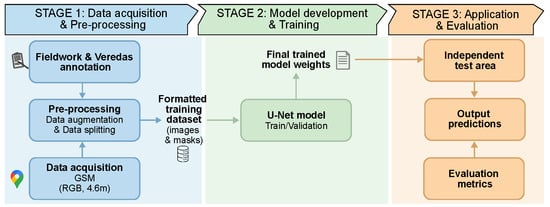
Figure 1. Proposed pipeline for the segmentation of mosaic images using a U-Net model.

2.1. Study Area

VED.SGF wetlands were selected using a hierarchical downscaling approach (Figure 2): (i) the Cerrado domain (noting that Veredas are not restricted to the Cerrado); (ii) the Sub-Middle São Francisco River Basin (247,518 km²); and (iii) the southwestern Chapadão do São Francisco in western Bahia. At this scale, two areas were defined: one for training and an adjacent area for testing (Figure 3A). This region was chosen for hosting the largest tabular Vereda wetlands in the Cerrado, linked to the São Francisco River Basin—northeastern Brazil’s most vital river system. Furthermore, these tabular wetlands are highly distinguishable, with well-defined spatial patterns that contrast sharply with surrounding Cerrado physiognomies.

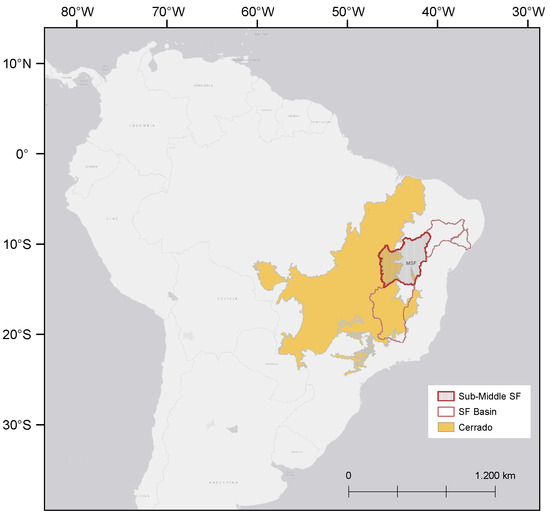
Figure 2. Geographic location of the study area within the South American landscape. The map highlights the Cerrado biome (yellow) and the Sub-middle São Francisco River Basin (red), detailing the sub-regional divisions of the São Francisco River Basin: High, Middle, Sub-Middle, and Low.

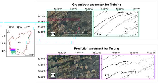
Figure 3. (A) Study area indicating the regions used for model training and independent testing. (B1) Preview of the RGB mosaic used for training. (B2) Corresponding expert-validated ground-truth binary mask used for model training. (C1) RGB mosaic of the independent testing area; and (C2) Ground-truth mask exclusively used for final model evaluation and error analysis (unseen during the training phase).

2.2. Data Acquisition

2.2.1. Satellite Imagery

Two subsets of the study area, representing typical VED.SGF wetlands, were selected to build the dataset: one for the training phase that corresponds to 7299.7 km² and another for independent testing with 8040.57 km² (Figure 3). While the training subset was used for model supervision (Figure 3B), the testing subset (Figure 3C) was reserved exclusively for final evaluation and error analysis, using a reference mask manually delineated by an expert to ensure an independent validation of the model’s performance. Although geographically adjacent, the testing area was strictly isolated to ensure statistical independence. This configuration allows the model to be validated within the same geological context, where anthropogenic patterns—such as irrigation pivots and distinct degradation stages—vary significantly over short distances, establishing a reliable baseline for the Cerrado domain. For each subset, mosaics of Google Maps satellite imagery were generated and exported as georeferenced GeoTIFF files.

The satellite tiles were downloaded between March and May 2021 using the Google Maps Static API, corresponding to the end of the wet season. Each image was captured at Zoom Level 15, providing an approximate spatial resolution of 4.6 m per pixel. At this zoom level, the resolution is determined by the Google Maps tiling system based on the latitude of the study area [42]. The images were then processed to remove unwanted elements, such as Google logos, before being converted into GeoTIFF format.

It is important to note that Google Maps imagery provides only RGB composites (red, green, and blue channels), rather than multispectral data. These images are orthorectified and visually consistent mosaics, making them suitable for DL–based segmentation. While the API does not provide the Near-Infrared (NIR) band or precise acquisition dates, our strategy focused on stable ecosystem features. We assumed that perennial plants (such as palm groves) and stable geomorphological patterns would provide more reliable visual patterns for the model than seasonal water pools. This approach leverages the U-Net’s ability to recognize textures and shapes that remain consistent across seasons, making the model compatible with widely available RGB data.

2.2.2. Fieldwork and Ground-Truth Annotation

To establish a robust basis for annotation, extensive fieldwork was conducted across vast areas of the Cerrado to refine qualitative knowledge at multiple scales—from their integration within landscape mosaics to geomorphological types and internal variation patterns. As part of this effort, a series of drone transects (DJI Mavic Air 2) equipped with 4K cameras were flown at approximately 30 m above ground level to document landscape patterns and validate visual signatures (Appendix A). This multi-scale assessment ensured that even the most complex tabular VED.SGF expressions were correctly identified, reaching a stage where no significant errors were detected in the pre-diagnosis of the targeted ecosystems.

Ground-truth data were produced through these field validation procedures and manual annotation of selected satellite images. Field specialists assisted the interpretation, ensuring ecological accuracy in the labeling process. With this level of understanding of the tabular Vereda expressions, polygons were subsequently delineated in Google Earth Engine to create the training (Figure 3B) and independent testing (Figure 3C) datasets. The wetlands within these images were manually delineated and converted into binary masks with two classes: VED.SGF (1) and background (0).

These binary masks served as reference data for training and evaluating the classification accuracy of the DL models. The ground-truth masks were carefully prepared through visual inspection to account for variations between the images, particularly due to differences in acquisition dates of Google Maps satellite imagery.

The initial size of the training dataset was determined empirically. After observing a high occurrence of false positives in preliminary predictions across the study area, the dataset was expanded by adding additional images with corresponding manually annotated masks. This iterative process improved model performance and ensured more robust generalization across the study region.

2.3. Deep Learning Framework

2.3.1. Model Architecture

The U-Net architecture [43], originally developed for biomedical image segmentation, has demonstrated strong performance in remote sensing tasks [28,36], including plant species classification [44] and forest type mapping [45], among other tasks.

The proposed architecture follows (Figure 4) an encoder–decoder structure with skip connections. The encoder captures context through convolutional blocks, each with two convolutional layers (kernel size $3\times 3$), batch normalization (BN) and Exponential Linear Unit (ELU) activation. A $2\times 2$ max pooling to increase feature depth. The decoder reconstructs spatial dimensions using transposed convolutions and $2\times 2$ convolutions to reduce feature channels. Skip connections concatenate feature maps from the encoder to the decoder to preserve fine-grained details. The final layer applies a $1\times 1$ convolution with a sigmoid activation for binary predictions (0 = background; 1 = VED.SGF).

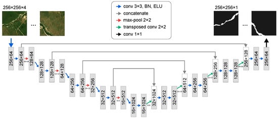
Figure 4. U-net architecture designed to receive imagery of $256\times 256$ and returns a prediction of the same dimension but with values 0 (background) and 1 (VED.SGF).

2.3.2. Model Training and Optimization

The proposed U-Net was trained from scratch using our domain-specific dataset. Weights were initialized using the He-normal method [46], as implemented in the Keras framework, to facilitate numerical stability and faster convergence. This ensures the network learns feature representations directly from the RGB mosaics, capturing the intrinsic patterns of Vereda.

During training, 75% of the dataset was allocated for training and 25% for validation. Random data augmentation was applied to increase model robustness, including flips, rotations (multiples of ${90}^{\circ }$), and scaling. Hyperparameters were set as follows: a learning rate of $0.001$, a maximum of 1000 epochs with early stopping (patience of 15 epochs), and a batch size of 10. This batch size was selected to ensure stable gradient estimation while remaining within the memory constraints of the hardware. Training was conducted on an NVIDIA Tesla T4 GPU (16 GB memory) with CUDA version 12.2, using TensorFlow 2.16.1 with the Keras API, provided by Google Colab environment.

2.3.3. Inference and Prediction Strategy

The input images were cropped into $256\times 256$ pixel chips, and the network outputs segmentation masks of the same dimensions. This size was selected as a standard benchmark in literature to balance spatial context with computational efficiency. During the inference phase, while training used non-overlapping chips, a sliding window approach with a 10% overlap (230-pixel stride) was applied during prediction to mitigate edge effects. These overlapping predictions were combined and binarized to ensure spatial continuity across tile boundaries.

2.3.4. Loss Function and Evaluation Metrics

The performance of the segmentation model was assessed using four widely adopted metrics for binary classification: F1-Score, Cohen’s Kappa (K), Average Accuracy, and Intersection over Union (IoU), also known as the Jaccard Index. In this context, positives refer to pixels classified as VED.SGF, and negatives refer to pixels classified as background. The terms $TP$ (True Positives), $TN$ (True Negatives), $FP$ (False Positives), and $FN$ (False Negatives) denote the number of correctly and incorrectly classified pixels with respect to the ground-truth masks.

The F1-score is the harmonic mean of precision and recall:

$$F1={\displaystyle \frac{2P\times R}{P+R}},$$

(1)

where precision (P) and recall (R) are defined as

$$P={\displaystyle \frac{TP}{TP+FP}},R={\displaystyle \frac{TP}{TP+FN}}.$$

(2)

Average Accuracy (Av. Acc.) represents the mean accuracy across the two classes (VED.SGF and background). Cohen’s Kappa (K) measures the agreement between predictions and ground-truth, adjusted for chance:

$$K={\displaystyle \frac{P_O-P_E}{1-P_E}},$$

(3)

where the observed accuracy is ${\displaystyle P_O=\frac{TP+TN}{TP+TN+FP+FN}}$, and $P_E$ is the expected accuracy by chance, computed as:

$$P_E=P_{\mathrm{VED}.\mathrm{SGF}}+P_{\mathrm{background}},$$

(4)

with:

$$P_{\mathrm{VED}.\mathrm{SGF}}={\displaystyle \frac{(TP+FN)(TP+FP)}{{(TP+TN+FP+FN)}^2}},$$

(5)

$$P_{\mathrm{background}}={\displaystyle \frac{(TN+FP)(TN+FN)}{{(TP+TN+FP+FN)}^2}}.$$

(6)

The IoU quantifies the overlap between the predicted segmentation and the ground-truth:

$$IoU={\displaystyle \frac{TP}{TP+FP+FN}}.$$

(7)

In addition, the loss function used during model training was the binary cross-entropy, which remains standard in segmentation tasks [19], which measures the pixel-wise error between predicted probabilities and ground-truth labels, and is expressed as:

$$L=-{\displaystyle \frac{1}{N}}\sum _{i=1}^N\left[y_{i}log\left({\widehat{y}}_i\right)+(1-y_i)log(1-{\widehat{y}}_i)\right],$$

(8)

where $y_i$ is the ground-truth label for pixel i, ${\widehat{y}}_i$ is the predicted probability, and N is the total number of pixels.

3. Results

3.1. Model Performance and Training Metrics

The U-Net model was trained for 53 epochs, achieving stable convergence around the 38th epoch, where the best-performing checkpoint was saved. As shown in Figure 5A, the loss function decreased rapidly with no signs of overfitting, reaching a minimum validation loss of $0.0461$, which indicates efficient optimization. Regarding computational costs, the training process was performed on an NVIDIA Tesla T4 GPU, totaling 4 h 4 min (averaging 275 s per epoch).

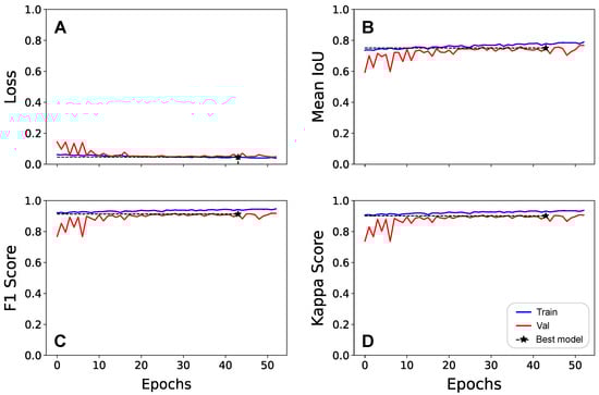
Figure 5. Training and validation curves for the U-Net model over 50 epochs, showing the evolution of (A) loss, (B) mean IoU, (C) F1-Score, and (D) Cohen’s Kappa. The y-axis represents the metric values, while the x-axis represents the number of epochs. The black marker indicates the best model checkpoint based on validation performance.

The mean IoU metric (Figure 5B) showed a steady increase, achieving $0.77$ for the training set and $0.76$ for the validation set. The minimal gap between the training and validation curves across all metrics (Figure 5B–D) demonstrates consistent convergence and robust generalization, confirming that the model learned the underlying patterns of the Cerrado wetlands rather than memorizing the training samples.

As detailed in Table 1, the model achieved high accuracy (94.95%) and a Cohen’s Kappa of 0.90 on the validation set, with an F1-score of 0.91. These results evidence excellent generalization with minimal performance drop, highlighting the model’s ability to accurately delineate VED.SGF wetlands across heterogeneous landscapes.

Table 1. Performance analysis of the trained U-Net model on training and validation sets for VED.SGF segmentation, situated alongside literature benchmarks. Values marked with (*) were calculated or adapted from the original studies for standardization.

Dataset	Author	Loss	IoU	F1	Kappa	Acc. (%)	Recall	Spec.
Validation	This study	0.046	0.76	0.91	0.90	94.95	—	—
Validation	Mainali et al. [36]	—	0.83	0.91 *	—	91.60	0.91	—
Validation	Bendini et al. [28]	—	0.14 *	0.24	0.17 *	79.00	0.58	0.80
Training	This study	0.042	0.77	0.94	0.93	96.46	—	—
Training	Bendini et al. [28]	—	0.58 *	0.72	0.71 *	97.00	0.73	0.98

3.2. Contextualization with Existing Literature

While a direct numerical comparison between studies is limited by differences in spatial resolution, sensors, and geographic contexts (e.g., USA vs. Brazil), it serves to contextualize our findings within the current state of the art. Thus, our model demonstrated consistent and robust performance across training and validation phases (Table 1).

Previous studies have made significant contributions to DL-based wetland mapping, though with different contexts, input data, and methodological approaches. Mainali et al. [36] conducted in the United States, focused on high-resolution mapping (1 m) using multispectral NAIP and Sentinel-2 imagery, combined with LiDAR-derived data and geomorphons. They implemented a U-Net architecture, achieving strong performance in training areas (precision of 96.5%, AUC of 95.2%), but showed limited spatial transferability to distant geographies. Bendini et al. [28] targeted Brazilian Veredas in the Cerrado, using Sentinel-2 imagery at 10 m resolution. They compared GEOBIA (an image processing method) with Random Forest and a fully convolutional U-Net. While the U-Net outperformed GEOBIA in transferability, overall results were modest (IoU = 0.14, F1 = 0.24), reflecting challenges due to coarser resolution and high landscape heterogeneity.

When situated alongside these benchmarks (Table 1), our model exhibits greater consistency and robustness for the Cerrado domain. It yielded a validation accuracy (94.95%) that stands competitively against both Mainali et al. [36] (91.60%) and Bendini et al. [28] (79.00%), with minimal drop between training and validation. While the IoU is slightly lower than the values reported by Mainali et al. [36], the combination of 4.6 m Google Maps imagery and a U-Net architecture provided a balanced trade-off between spatial detail and computational efficiency, enabling reliable mapping of VED.SGF areas in a complex biome.

3.3. Spatial Generalization on Unseen Test Areas

After the initial training and validation phases, the U-Net model was applied to an unseen test area (Figure 3C), completely excluded from the training and validation datasets, to assess its generalization capability in a real-world scenario. While validation metrics are useful for benchmarking against existing literature, we consider the performance on this independent area to be the authoritative assessment of the model’s operational capability. Consequently, the metrics derived from this unseen region are those formally reported as the model’s effective accuracy for regional mapping and future monitoring tasks.

To provide a rigorous quantitative evaluation, the model’s predictions were compared against a dedicated ground-truth mask specifically reserved for this unseen region (Figure 3C). The input satellite imagery maintained the same parameters used during training, with a spectral resolution of 4.6 m. Regarding the computational efficiency, the model processed the entire test area ($8040.57$ km²) in 13 min and 38 s using a sliding window approach, demonstrating its scalability for large-scale applications.

Figure 6 illustrates the VED.SGF segmentation for the selected test region, with predicted areas highlighted in magenta.

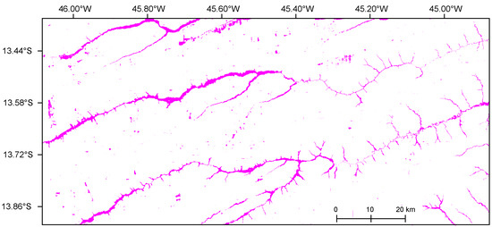
Figure 6. Predicted wetland segmentation in the test area, with magenta representing VED.SGF.

The model’s performance was evaluated through both quantitative metrics and a spatial qualitative analysis. The quantitative results, summarized in Table 2, confirm a robust performance in complex landscape classification, with a Kappa Index of $0.837$ and an F1-Score of $0.843$. The detailed distribution of pixel-wise classifications is provided in the confusion matrix (Table 3), which highlights a high sensitivity, with a Recall of $0.936$. This metric indicates that the model successfully identified 213.72 km² (2.66%) of Veredas, while omitting only $14.61$ km² (0.18%) in terms of total area. Although the Precision of $0.766$ reflects some degree of over-prediction, amounting to $65.30$ km² (0.81%) of False Positives, the Specificity remains remarkably high ($0.992$). The specific nature and spatial distribution of these quantified errors are further examined in the following qualitative analysis.

Table 2. Quantitative performance metrics of the U-Net model on the unseen test area.

Metric	Value
IoU	0.728
F1-Score	0.843
Kappa Coefficient	0.837
Accuracy	0.990
Recall	0.936
Precision	0.766
Specificity	0.992

Table 3. Confusion matrix results for the unseen test area expressed in square kilometers (km²).

Observed/Predicted	Vereda	Non-Vereda	Total Predicted
Vereda	$213.72$ (TP)	$65.30$ (FP)	$279.02$
Non-Vereda	$14.61$ (FN)	7746.66 (TN)	7761.27
Total observed	$228.33$	7811.96	8040.29

3.4. Qualitative Visual and Error Analysis

Overall, the model achieved visually coherent delineations, accurately mapping VED.SGF areas across heterogeneous landscapes. As shown in the top panel from Figure 7), the model maintains structural connectivity across the 8040 km² domain, with errors appearing as localized clusters rather than systemic bias. The results confirm that the architecture prioritized stable geometric features—such as dendritic and elongated shapes—over transient spectral variations.

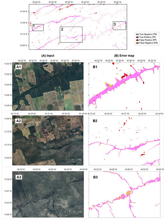
Figure 7. Qualitative assessment and error analysis of the U-Net segmentation results. Top-panel showing an overview of the test area showing the spatial distribution of True Positives, False Positives, and False Negatives; (A1–A3) Original high-resolution RGB mosaics; (B1–B3) Pixel-wise error maps classification: TP (light magenta) representing correct wetland identification; FP (red) indicating misclassifications; FN (yellow) showing omitted wetland areas; and True Negatives (TN, white background) representing correctly identified non-wetland areas.

To provide a spatial diagnostic of the quantitative discrepancies (False Positives and False Negatives) reported in reported in Section 3.3 and Table 3, three subsets were selected representing distinct environmental contexts: preserved wetlands, anthropogenic interference, and complex drainage networks. These samples illustrate where spectral or textural similarities may lead to localized misclassifications.

• Preserved wetlands (Figure 7(A1,B1)): In regions with minimal anthropogenic influence, the model demonstrated high fidelity in delineating the elongated and dendritic morphology of wetlands. The high density of True Positives indicates that our model effectively captures the intrinsic spatial structures of the Cerrado from RGB imagery, confirming that spatial geometry is a reliable proxy for wetland identification.
• Anthropogenic interference (Figure 7(A2,B2)): The primary limitation observed involves spectral confusion with center-pivot irrigation systems. These “anthropogenic impostors” maintain high vegetation vigor and moisture, producing spectral responses in the visible range similar to natural Veredas. The well-defined circular geometry of these False Positives (red) suggests that incorporating auxiliary descriptors, such as shape or topographic information, may further improve classification accuracy.
• Complex drainage networks (Figure 7(A3,B3)): In areas with dense, sinuous networks and high fragmentation, the model remained robust. False Negatives (yellow) are mostly limited to extremely narrow wetland fringes. These omissions occur where the wetland width approaches the pixel resolution limit (4.6 m), representing a boundary effect rather than a failure in pattern recognition.

4. Discussion

The proposed U-Net model showed strong and stable performance, with high accuracy and balanced generalization across training, validation, and the unseen test area. Visual inspection confirmed reliable delineations even in complex regions, showing that moderate-resolution imagery (4.6 m) can effectively support DL-based wetland mapping in heterogeneous Cerrado landscapes. While the validation IoU reached 0.76, the model sustained a robust IoU of 0.728 in a completely independent test area of 8040 km². This slight decrease is expected in real-world scenarios and demonstrates that the model achieved high generalization without suffering from overfitting. The model’s computational efficiency underscores its operational potential for large-scale monitoring. Completing the training process in approximately 4 h on a single mid-range GPU indicates accessibility for regional mapping, while the high inference throughput—processing over 8000 km² in under 14 min (approximately 1.1 s per km²)—demonstrates its scalability for the entire Cerrado domain.

When situated alongside previous studies, our approach exhibits competitive performance with specific operational advantages. For instance, Mainali et al. [36], using 1 m imagery and additional LiDAR data, achieved a higher IoU (0.83) but a lower overall accuracy (91.6%) than our formal test results (99.0%), suggesting that our approach yielded highly reliable predictions even without very high-resolution imagery. Bendini et al. [28], conversely, faced spatial precision limits with 10 m Sentinel-2 imagery, yielding modest IoU (0.14). These variations highlight that our intermediate resolution and specialized training provide a superior balance between precision and computational efficiency for the Cerrado domain.

While multispectral and SAR data would likely enhance spectral depth, the reliance on high-resolution RGB imagery was a strategic choice for this initial stage. Our experiments show that RGB data is reliable because the main visual signs of Veredas—such as their narrow, dendritic shapes and permanent palm groves—remain consistent throughout the year. Our strategy focused on these stable features to ensure that the acquisition date of the image (whether from the dry or rainy season) would not compromise the results. This allowed the U-Net to maintain its accuracy even without precise satellite acquisition dates or NIR bands, establishing a computationally light and accessible baseline. By prioritizing these stable geometries over infrared bands, we ensured the methodology remains seasonally robust and ready for geographic expansion across the continental dimensions of the Brazilian Cerrado.

This study also introduces the second annotated dataset for VED.SGF wetlands (following Brasil et al. [18]), providing a valuable resource for future research and benchmarking. However, the current annotated area coverage (∼7300 km²), represents only a fraction of the São Francisco basin, which may limit sample diversity. Qualitative analysis indicates that while the model captures complex dendritic geometries, localized false positives occur primarily in center-pivot irrigation systems and, occasionally, in topographic shadows. Conversely, omissions tend to occur in extremely narrow wetland fringes where patterns approach the pixel resolution limit. These geomorphological and anthropogenic “impostors” are key challenges to be mitigated in future iterations by including digital elevation models and multispectral sensors.

Expanding the dataset is essential to encompass the full range of Vereda types—complex systems functioning as macro-community organisms—and their various stages of anthropogenic distortion. This expansion must also broaden the environmental contexts sampled, as their floristic composition varies across ecoregions. Such variability introduces a significant learning challenge: ecologically equivalent landscapes acting as misleading analogues (“false homologues”) that the model must eventually learn to distinguish.

Finally, the use of a trained-from-scratch U-Net backbone eliminates the need for manual feature engineering and supports scalability to other biomes. By avoiding the use of generic, non-specialized pre-trained weights (e.g., ImageNet [37]), the model was able to learn features specifically tailored to the complex geometries of VED.SGF wetlands. Overall, this work demonstrates that combining U-Net with moderate-resolution imagery provides a practical and accurate solution for mapping wetlands in complex and underexplored ecosystems, supporting data-driven conservation strategies.

5. Conclusions

The progress achieved in this study should be understood as an initial step within a broader research program aimed at mapping functional landscape units in the Cerrado domain. Even within Vereda wetlands, substantial challenges remain and will require continued investment and methodological refinement. Our initial dataset covers approximately 7300 km² of the São Francisco Basin representing only a small fraction of the total wetland distribution in South America, which extends beyond the Cerrado into the Pantanal and Caatinga domains. Future efforts should therefore prioritize geographic expansion, the creation of Veredas subclasses, and the incorporation of distinct degradation stages.

To support these future efforts, we provide the public availability of our model weights and annotated data, which were designed to map the complex landscapes of wetlands and riparian forests in the Cerrado. This establishes a foundation for reproducible research and standardized benchmarks in the Cerrado. In summary, the main contributions of this study are (i) the development of a specialized U-Net model whose weights are optimized for domain-specific transfer learning; (ii) the release of high-quality, field-validated annotations that help fill the gap of labeled data for this biome; and (iii) the establishment of a scalable pipeline capable of rapid processing (over 1 km²/s), enabling efficient ecological assessment in regions under intense agricultural pressure.

The model achieved robust performance, as formally demonstrated by the results in the unseen test area (IoU = 0.728; F1-score = 0.843; Kappa = 0.837), with stable generalization that confirms the potential of our deep learning approach for heterogeneous ecosystems. These resources serve as a pre-trained foundation for transfer learning, enabling adaptation to other wetland types, regions, or datasets with comparable spectral and spatial characteristics. Expanding annotated coverage and integrating multispectral and/or SAR data will be essential to enhance robustness, scalability, and overall accuracy.

From an ecological and conservation perspective, precise and dynamic mapping of Vereda wetlands provides critical support for biodiversity management in the Cerrado—vast savanna-like landscapes of Central Brazil increasingly exposed to anthropogenic pressures, particularly large-scale agricultural expansion.

Future research should also explore Explainable AI (XAI) approaches to improve model interpretability, more advanced architectures such as DeepLabV3+ and Transformer-based models, and near real-time monitoring frameworks for seasonal and long-term landscape dynamics. Such developments will further strengthen the role of deep learning in ecological monitoring and evidence-based decision-making.

Appendix A.1. Panoramic Photographs from São Francisco Basin

To build a critical understanding of Vereda wetlands, extensive fieldwork was conducted across vast areas of the Cerrado to refine qualitative knowledge at multiple scales—from their integration within landscape mosaics to smaller-scale assessments of geomorphological types and internal variation patterns. As part of this effort, a series of drone transects (DJI Mavic Air 2) equipped with 4K cameras were flown approximately 30 m above ground level to document the observed landscape patterns (Figure A1). After extensive fieldwork testing of predictions based on Google Earth imagery, followed by validation exercises, we reached a stage in which no significant errors were detected in the pre-diagnosis, particularly for the tabular type of VED.SGF. With this level of understanding of the tabular Vereda expressions, polygons were subsequently delineated in Google Earth Engine as input data for model training.

Figure A1. Drone imagery of Vereda wetlands in the São Francisco Basin, Brazilian Midwest. (A) Oblique view showing transitions from flooded grasslands to palm-dominated vegetation along groundwater discharge zones. (B) Nadir view highlighting sinuous drainage channels bordered by dense vegetation within open wet grasslands.

Figure A1. Drone imagery of Vereda wetlands in the São Francisco Basin, Brazilian Midwest. (A) Oblique view showing transitions from flooded grasslands to palm-dominated vegetation along groundwater discharge zones. (B) Nadir view highlighting sinuous drainage channels bordered by dense vegetation within open wet grasslands.

References

- Zedler, J.B.; Kercher, S. Wetland Resources: Status, Trends, Ecosystem Services, and Restorability. Annu. Rev. Environ. Resour. 2005, 30, 39–74. [Google Scholar] [CrossRef]
- Vörösmarty, C.J.; McIntyre, P.B.; Gessner, M.O.; Dudgeon, D.; Prusevich, A.; Green, P.; Glidden, S.; Bunn, S.E.; Sullivan, C.A.; Liermann, C.R.; et al. Global Threats to Human Water Security and River Biodiversity. Nature 2010, 467, 555–561. [Google Scholar] [CrossRef] [PubMed]
- Mitsch, W.J.; Gosselink, J.G.; Anderson, C.J.; Fennessy, M.S. Wetlands, 6th ed.; Wiley: Hoboken, NJ, USA, 2023. [Google Scholar]
- Hofmann, G.S.; Weber, E.J.; Bastazini, V.A.G.; Rossato, D.R.; Franco, A.C.; Granada, C.E.; Kaminski, L.A.; Ubaid, F.K.; Leandro-Silva, V.; Borges-Martins, M.; et al. Climate Change in the Brazilian Cerrado: A Looming Threat to Terrestrial Biodiversity. WIREs Clim. Change 2025, 16, e70022. [Google Scholar] [CrossRef]
- Dudgeon, D. Multiple Threats Imperil Freshwater Biodiversity in the Anthropocene. Curr. Biol. 2019, 29, R960–R967. [Google Scholar] [CrossRef]
- Fluet-Chouinard, E.; Stocker, B.D.; Zhang, Z.; Malhotra, A.; Melton, J.R.; Poulter, B.; Kaplan, J.O.; Goldewijk, K.K.; Siebert, S.; Minayeva, T.; et al. Extensive Global Wetland Loss over the Past Three Centuries. Nature 2023, 614, 281–286. [Google Scholar] [CrossRef]
- Harrison, I.; Abell, R.; Darwall, W.; Thieme, M.L.; Tickner, D.; Timboe, I. The Freshwater Biodiversity Crisis. Science 2018, 362, 1369. [Google Scholar] [CrossRef]
- Myers, N.; Mittermeier, R.A.; Mittermeier, C.G.; Fonseca, G.A.B.; Kent, J. Biodiversity Hotspots for Conservation Priorities. Nature 2000, 403, 853–858. [Google Scholar] [CrossRef]
- Oliveira, P.S.; Marquis, R.J. The Cerrados of Brazil: Ecology and Natural History of a Neotropical Savanna; Columbia University Press: New York, NY, USA, 2002. [Google Scholar]
- Latrubesse, E.M.; Arima, E.; Ferreira, M.E.; Nogueira, S.H.; Wittmann, F.; Dias, M.S.; Dagosta, F.C.P.; Bayer, M. Fostering Water Resource Governance and Conservation in the Brazilian Cerrado Biome. Conserv. Sci. Pract. 2019, 1, e77. [Google Scholar] [CrossRef]
- Ferreira, M.E.; Nogueira, S.H.M.; Latrubesse, E.M.; Macedo, M.N.; Callisto, M.; Bezerra, N.; Neto, J.F.; Fernandes, G.W. Dams Pose a Critical Threat to Rivers in Brazil’s Cerrado Hotspot. Water 2022, 14, 3762. [Google Scholar] [CrossRef]
- Pereira, C.C.; Fernandes, G.W. Cerrado Conservation Is Key to the Water Crisis. Science 2022, 377, 270. [Google Scholar] [CrossRef]
- Alencar, A.; Z. Shimbo, J.; Lenti, F.; Balzani Marques, C.; Zimbres, B.; Rosa, M.; Arruda, V.; Castro, I.; Fernandes Márcico Ribeiro, J.; Varela, V.; et al. Mapping Three Decades of Changes in the Brazilian Savanna Native Vegetation Using Landsat Data Processed in the Google Earth Engine Platform. Remote Sens. 2020, 12, 924. [Google Scholar] [CrossRef]
- Durigan, G.; Munhoz, C.B.; Zakia, M.J.B.; Oliveira, R.S.; Pilon, N.A.L.; Valle, R.S.T.; Walter, B.M.T.; Honda, E.A.; Pott, A. Cerrado Wetlands: Multiple Ecosystems Deserving Legal Protection. Perspect. Ecol. Conserv. 2022, 20, 185–196. [Google Scholar] [CrossRef]
- Machado, R.B.; Sano, L.M.S.A.; Bustamante, M.M.C. Why Is It So Easy to Undergo Devegetation in the Brazilian Cerrado? Perspect. Ecol. Conserv. 2024, 22, 209–212. [Google Scholar] [CrossRef]
- Salmona, Y.B.; Matricardi, E.A.T.; Skole, D.L.; Silva, J.F.A.; Coelho Filho, O.d.A.; Pedlowski, M.A.; Sampaio, J.M.; Castrillón, L.C.R.; Brandão, R.A.; Silva, A.L.; et al. A Worrying Future for River Flows in the Brazilian Cerrado. Sustainability 2023, 15, 4251. [Google Scholar] [CrossRef]
- Beer, F.; Munhoz, C.B.R.; Couwenberg, J.; Horák-Terra, I.; Fonseca, L.M.G.; Bijos, N.R.; Nunes Da Cunha, C.; Wantzen, K.M. Peatlands in the Brazilian Cerrado: Insights into Knowledge, Status and Research Needs. Perspect. Ecol. Conserv. 2024, 22, 260–269. [Google Scholar] [CrossRef]
- Brasil, M.C.O.; Magalhães-Filho, R.; Espírito-Santo, M.M.; Leite, M.E.; Veloso, M.D.M.; Falcão, L.A.D. Land-Cover Changes and Drivers of Palm Swamp Degradation in Southeastern Brazil from 1984 to 2018. Appl. Geogr. 2021, 137, 102604. [Google Scholar] [CrossRef]
- Hasan, K.R.; Tuli, A.B.; Khan, M.A.M.; Kee, S.H.; Samad, M.A.; Nahid, A.A. Deep-Learning-Based Semantic Segmentation for Remote Sensing. IEEE J. Sel. Top. Appl. Earth Obs. Remote Sens. 2024, 17, 1390–1418. [Google Scholar] [CrossRef]
- He, K.; Zhang, X.; Ren, S.; Sun, J. Deep Residual Learning for Image Recognition. In Proceedings of the IEEE Conference on Computer Vision and Pattern Recognition, Las Vegas, NV, USA, 27–30 June 2016; pp. 770–778. [Google Scholar] [CrossRef]
- Simonyan, K.; Zisserman, A. Very Deep Convolutional Networks for Large-Scale Image Recognition. In Proceedings of the International Conference on Learning Representations, San Diego, CA, USA, 7–9 May 2015. [Google Scholar] [CrossRef]
- Fan, L.; Wang, W.C.; Zha, F.; Yan, J. Exploring New Backbone and Attention Module for Semantic Segmentation. IEEE Access 2018, 6, 71566–71580. [Google Scholar] [CrossRef]
- Mahdianpari, M.; Salehi, B.; Mohammadimanesh, F.; Homayouni, S.; Gill, E. The First Wetland Inventory Map of Newfoundland at a Spatial Resolution of 10 m Using Sentinel-1 and Sentinel-2 Data on the Google Earth Engine Cloud Computing Platform. Remote Sens. 2019, 11, 43. [Google Scholar] [CrossRef]
- Onojeghuo, A.O.; Onojeghuo, A.R.; Cotton, M.; Potter, J.; Jones, B. Wetland Mapping with Multi-Temporal Sentinel-1 and Sentinel-2 Imagery and LiDAR Data in the Grassland Natural Region of Alberta. GIScience Remote Sens. 2021, 58, 999–1021. [Google Scholar] [CrossRef]
- Mohseni, F.; Amani, M.; Mohammadpour, P.; Kakooei, M.; Jin, S.; Moghimi, A. Wetland Mapping in Great Lakes Using Sentinel-1/2 Time-Series Imagery and DEM Data in Google Earth Engine. Remote Sens. 2023, 15, 3495. [Google Scholar] [CrossRef]
- Bakkestuen, V.; Venter, Z.; Ganerød, A.J.; Framstad, E. Delineation of Wetland Areas in South Norway from Sentinel-2 Imagery and LiDAR Using TensorFlow, U-Net, and Google Earth Engine. Remote Sens. 2023, 15, 1203. [Google Scholar] [CrossRef]
- Mohammadimanesh, F.; Salehi, B.; Mahdianpari, M.; Gill, E.; Molinier, M. A New Fully Convolutional Neural Network for Semantic Segmentation of Polarimetric SAR Imagery in Complex Land Cover Ecosystem. Isprs J. Photogramm. Remote Sens. 2019, 154, 151–164. [Google Scholar] [CrossRef]
- Bendini, H.N.; Fonseca, L.M.G.; Maretto, R.V.; Matosak, B.M.; Taquary, E.C.; Simões, P.S.; Haidar, R.F.; Valeriano, D.D.M. Exploring a Deep Convolutional Neural Network and GEOBIA for Automatic Recognition of Brazilian Palm Swamps (Veredas) Using Sentinel-2 Optical Data. In Proceedings of the IEEE International Geoscience and Remote Sensing Symposium (IGARSS), Brussels, Belgium, 12–16 July 2021. [Google Scholar] [CrossRef]
- Peña, F.J.; Hübinger, C.; Payberah, A.H.; Jaramillo, F. DeepAqua: Semantic Segmentation of Wetland Water Surfaces with SAR Imagery using Deep Neural Networks without Manually Annotated Data. Int. J. Appl. Earth Obs. Geoinf. 2024, 126, 103624. [Google Scholar] [CrossRef]
- Panboonyuen, T.; Jitkajornwanich, K.; Lawawirojwong, S.; Srestasathiern, P.; Vateekul, P. Semantic Segmentation on Remotely Sensed Images Using an Enhanced Global Convolutional Network with Channel Attention and Domain Specific Transfer Learning. Remote Sens. 2019, 11, 83. [Google Scholar] [CrossRef]
- Wurm, M.; Stark, T.; Zhu, X.X.; Weigand, M.; Taubenböck, H. Semantic Segmentation of Slums in Satellite Images using Transfer Learning on Fully Convolutional Neural Networks. Isprs J. Photogramm. Remote Sens. 2019, 150, 59–69. [Google Scholar] [CrossRef]
- Bhatnagar, S.; Gill, L.; Ghosh, B. Drone Image Segmentation Using Machine and Deep Learning for Mapping Raised Bog Vegetation Communities. Remote Sens. 2020, 12, 2602. [Google Scholar] [CrossRef]
- Saltiel, T.; Dennison, P.; Campbell, M.; Thompson, T.; Hambrecht, K. Tradeoffs between UAS Spatial Resolution and Accuracy for Deep Learning Semantic Segmentation Applied to Wetland Vegetation Species Mapping. Remote Sens. 2022, 14, 2703. [Google Scholar] [CrossRef]
- Guan, X.; Wang, D.; Wan, L.; Zhang, J. Extracting Wetland Type Information with a Deep Convolutional Neural Network. Comput. Intell. Neurosci. 2022, 2022, 5303872. [Google Scholar] [CrossRef] [PubMed]
- Chen, Z.; Chen, J.; Yue, Y.; Lan, Y.; Ling, M.; Li, X.; You, H.; Han, X.; Zhou, G. Tradeoffs among Multi-Source Remote Sensing Images, Spatial Resolution, and Accuracy for the Classification of Wetland Plant Species and Surface Objects based on the MRS_DeepLabV3+ Model. Ecol. Inform. 2024, 81, 102594. [Google Scholar] [CrossRef]
- Mainali, K.; Evans, M.; Saavedra, D.; Mills, E.; Madsen, B.; Minnemeyer, S. Convolutional Neural Network for High-Resolution Wetland Mapping with Open Data: Variable Selection and the Challenges of a Generalizable Model. Sci. Total Environ. 2023, 861, 160622. [Google Scholar] [CrossRef]
- Deng, J.; Dong, W.; Socher, R.; Li, L.J.; Li, K.; Fei-Fei, L. ImageNet: A Large-Scale Hierarchical Image Database. In Proceedings of the IEEE Conference on Computer Vision and Pattern Recognition, Miami, FL, USA, 20–25 June 2009; pp. 248–255. [Google Scholar] [CrossRef]
- Yan, Z.; Zheng, H.; Li, Y. Detail Injection with Heterogeneous Composite Backbone Network for Object Detection. Multimed. Tools Appl. 2022, 81, 11621–11637. [Google Scholar] [CrossRef]
- Shi, B.; Zhang, X.; Wang, Y.; Dai, W.; Zou, J.; Xiong, H. MENSA: Multi-Dataset Harmonized Pretraining for Semantic Segmentation. IEEE Trans. Multimed. 2025, 27, 2127–2140. [Google Scholar] [CrossRef]
- Liu, R.; Liang, J.; Yang, J.; Hu, M.; He, J.; Zhu, P.; Zhang, L. DHSNet: Dual Classification Head Self-Training Network for Cross-Scene Hyperspectral Image Classification. IEEE Trans. Geosci. Remote Sens. 2025, 63, 5534515. [Google Scholar] [CrossRef]
- Liu, R.; Zhou, M.; Yang, J.; Wang, J. Adaptive Smooth Adversarial Learning for Cross-Domain Hyperspectral Image Classification. IEEE Trans. Geosci. Remote Sens. 2025, 63, 5529017. [Google Scholar] [CrossRef]
- Google. Google Maps Platform: Static Maps API; Online Documentation; Google: Mountain View, CA, USA, 2025. [Google Scholar]
- Ronneberger, O.; Fischer, P.; Brox, T. U-Net: Convolutional Networks for Biomedical Image Segmentation. In Medical Image Computing and Computer-Assisted Intervention—MICCAI 2015; Springer: Cham, Switzerland, 2015; pp. 234–241. [Google Scholar] [CrossRef]
- Kattenborn, T.; Eichel, J.; Fassnacht, F.E. Convolutional Neural Networks Enable Efficient, Accurate and Fine-Grained Segmentation of Plant Species and Communities from High-Resolution UAV Imagery. Sci. Rep. 2019, 9, 17656. [Google Scholar] [CrossRef]
- Wagner, F.H.; Sanchez, A.; Tarabalka, Y.; Lotte, R.G.; Ferreira, M.P.; Aidar, M.P.M.; Gloor, E.; Phillips, O.L.; Aragão, L.E.O.C. Using the U-Net Convolutional Network to Map Forest Types and Disturbance in the Atlantic Rainforest with very High Resolution Images. Remote Sens. Ecol. Conserv. 2019, 5, 360–375. [Google Scholar] [CrossRef]
- He, K.; Zhang, X.; Ren, S.; Sun, J. Delving Deep into Rectifiers: Surpassing Human-Level Performance on ImageNet Classification. arXiv 2015, arXiv:1502.01852. [Google Scholar] [CrossRef]
Disclaimer/Publisher’s Note: The statements, opinions and data contained in all publications are solely those of the individual author(s) and contributor(s) and not of MDPI and/or the editor(s). MDPI and/or the editor(s) disclaim responsibility for any injury to people or property resulting from any ideas, methods, instructions or products referred to in the content. |
© 2026 by the authors. Licensee MDPI, Basel, Switzerland. This article is an open access article distributed under the terms and conditions of the Creative Commons Attribution (CC BY) license.