Forecasting Diurnal Sea Surface Temperature Variation in the Equatorial Pacific Based on Improved CoTCN

Highlights

What are the main findings?

• To forecast diurnal sea surface temperature (SST) variation (DSV), CoTCN-DSV is proposed based on CoTCN and an improved loss function including the maximum and minimum SST over the equatorial Pacific.
• CoTCN-DSV has the good ability (good skill and generalization) to forecast DSV due to the perfect representation of the maximum and minimum SSTs in a day.

What are the implications of the main findings?

• CoTCN-DSV has the potential to forecast extreme values for different scenarios.
• High-quality data are important for deep learning models to advance the forecast accuracy.

Abstract

The diurnal sea surface temperature variation (DSV) influences atmospheric convection and precipitation through air–sea interactions in the equatorial Pacific. Deep learning-based DSV forecasting has been less explored compared to traditional methods, presenting the potential for a substantial leap in forecast accuracy. In this study, a forecast model is developed for 24 h DSV in the equatorial Pacific using an improved coupled Transformer-CNN (CoTCN-DSV) by incorporating a new loss function including maximal and minimal values. The CoTCN-DSV forecasts diurnal variation in SST at the interval of 3 h based on 3 h SST from the WHOI dataset. The CoTCN-DSV captures DSV well with root mean square error (RMSE) of DSA below 0.03 °C/0.13 °C at 3 h/12 h lead times and maintains high forecast skill with the temporal correlation coefficient (R) of 0.78 at the lead times of 12 h in the equatorial Pacific. The CoTCN-DSV reduces RMSE for daily max/min SST by 10.9% and 12.8% due to replacing the new loss function, then significantly improving DSV forecast. There are systematic SST biases in the WHOI dataset and this leads to relatively large RMSEs when DSV forecasts trained using WHOI are evaluated against TAO observations. Replaced WHOI SST by TAO SST, the forecasted DSA RMSE by CoTCN-DSV is reduced by an average of 43%. This confirms that the CoTCN-DSV has good generalization ability and high-quality data are important to advance the forecast accuracy. These finding show that CoTCN-DSV has the potential to forecast extreme values for different scenarios.

1. Introduction

Sea surface temperature (SST) is one of the most important indicators of climate variability [1]. Driven by solar radiation, wind forcing, and tidal currents, SST exhibits pronounced diurnal variability [2,3]. Diurnal SST variations (denoted as DSV) regulate air–sea interaction processes [4]. In tropics, DSV is also closely associated with the phase locking of the El Niño-Southern Oscillation (ENSO) [5]. Moreover, DSV affects the spatiotemporal distribution of phytoplankton and fisheries resource assessment. Therefore, accurate and high-frequency DSV forecast is particularly critical, especially over the equatorial Pacific, a key region for ENSO development.

Traditional approaches for forecasting DSV can be categorized into three main types [6]. Empirical parametric models typically offer high computational efficiency but rely primarily on statistical relationships and lack a strong physical basis [2,7]. Bulk models are more physically based than empirical models, yet they often omit key dynamical processes involved in air–sea interactions [8,9,10,11]. Dynamical models possess clear physical interpretations but require very-high vertical resolution and a large number of parameters, and also entail high computational complexity [12,13,14].

In recent years, artificial intelligence methods (including machine learning) such as random forests [15], support vector machines (SVM) [16] and neural networks [17] have demonstrated significant improvements in SST forecasts across various time scales. In particular, deep learning models based on multi-layer neural networks exhibit strong forecast capability when handling large-scale, high-dimensional datasets, enabling effective extraction of SST variability characteristics. At monthly and seasonal scales, gated recurrent unit (GRU) neural networks have been successfully applied to monthly and seasonal SST forecasting, showing good robustness [18]. In addition, hybrid architectures such as UNet-LSTM, which combine multi-scale spatial feature extraction with temporal dependency modeling, have achieved accurate forecasts of global monthly mean SST [19]. At daily scales, the introduction of advanced architectures—including long short-term memory (LSTM), Convolutional Neural Network (CNN), ConvLSTM, graph convolutional networks (GCNs), and Transformer models—has significantly enhanced SST forecast performance [20,21,22,23,24]. Most of these studies focus on applying deep learning to daily forecast, whereas investigations that specifically target DSV in a day receive less attention.

The equatorial Pacific exhibits the pronounced SST pattern including warm pool in the western part and cold tongue in the eastern part, which is the key region for ENSO events [25]. DSV can induce strong air–sea interaction and modulate or interact with ENSO. Machine learning approaches such as the LDS-XGBoost model have been applied to forecast diurnal SST amplitudes (denoted as DSA) for multiple tropical stations [26], achieving better performance than empirical models [27], RBF neural networks [28], random forests, and stacking ensembles [29]. Nevertheless, such findings are primarily based on station-based observation data and utilize traditional machine learning approaches which are frequently inadequate for modeling the spatial correlations in SST. Deep learning models can be a good choice for forecasting DSV over the equatorial Pacific. To capture DSV well, the maximal and minimal values should be described well in the first step. Therefore, to advance DSV forecasting in the equatorial Pacific, it is imperative to develop a deep learning network that can not only characterize spatiotemporal patterns but also specifically enhance the representation of key extremes—namely, the maximum and minimum values.

In this study, we developed a network to forecast DSV in the equatorial Pacific based on a coupled Transformer-CNN (CoTCN, [30]). To enhance the capability of capturing SST extreme values in a day, a loss function incorporating the maximum and minimum values was designed. Using this network, forecasted diurnal variations in SST are systematically investigated. The paper is organized as follows: Section 1 introduces the study background and provides the review of previous studies briefly. Section 2 describes the study region, datasets, and methodology. Section 3 presents forecast maximum and minimum SST, DSA, and evaluation using different datasets. Section 4 provides the discussion. Section 5 provides conclusions.

2. Data and Methods

2.1. Study Area and Data

The study focuses on the equatorial Pacific, spanning 15°S–15°N and 130°E–80°W. The primary dataset used is the NOAA–WHOI climate data record, which combines high-resolution Advanced Very High Resolution Radiometer (AVHRR) SST observations with simulations of diurnal variations. The dataset provides SST at 3 h intervals, corresponding to eight time points per day (UTC 01:30, 04:30, 07:30, 10:30, 13:30, 16:30, 19:30, and 22:30), with a spatial resolution of 0.25° × 0.25°. The study period covers 31 years, from 1 January 1988 to 31 December 2018. The data can download from https://www.ncei.noaa.gov/data/sea-surface-temperature-whoi/access/ (accessed on 14 August 2025).

To further evaluate the SST from WHOI dataset and the diurnal SST forecasts, in situ observations from the Tropical Atmosphere Ocean (TAO) project are also employed, with a temporal span matching that of the WHOI-SST testing set. The TAO array, designed to monitor air–sea interaction processes in the tropical Pacific, consists of 55 moored buoys distributed primarily between 8°S and 9°N and 165°E–95°W. We employed 10 min SST data to validate the forecast data which can be downloaded from https://www.pmel.noaa.gov/tao/drupal/disdel/ (accessed on 4 November 2025).

2.2. Data Preprocessing

Before training, the SST data from WHOI dataset were clipped based on the spatial extent of the study region and chosen according to good quality data in which only valid observation was used. Missing values were subsequently filled using a forward-fill method along the temporal dimension in pandas.

To accelerate the convergence, stabilize gradients, and mitigate the issues of gradient explosion or vanishing, the data were standardized using the Z-score method. The calculation formula is as follows:

$$\overline{x}={\displaystyle \frac{1}{n}}{\displaystyle \sum _{i=1}^n{x}_i}$$

(1)

$$\sigma =\sqrt{{\displaystyle \frac{1}{n}}{\displaystyle \sum _{i=1}^n{(x_i-\overline{x})}^2}}$$

(2)

$$x_{scaled}={\displaystyle \frac{x-\overline{x}}{\sigma }}$$

(3)

where $x_i$ denotes the input sequence, $n$ represents the total number of samples in the input sequence, $\overline{x}$ is the mean of the input sequence, $\sigma$ is the standard deviation, and $X_{scaler}$ is the standardized value.

To compare the impact of different input datasets, selected WHOI-SST grid values were replaced using TAO buoy observations. For each buoy location, the four nearest WHOI grid points were identified, and the buoy SST value at each time step was directly assigned to these neighboring grid cells when valid observations were available.

For validation against TAO observations, the forecasts were bilinearly interpolated to the buoy locations using the four surrounding grid points. If any of these four grid points contained missing values, the interpolated value was calculated as the mean of the remaining valid grid points. This approach ensures a consistent spatial comparison between gridded forecasts and point-based buoy observations.

2.3. Building DSV Network

Given that the CoTCN has been demonstrated to outperform various deep learning models in short-term global SST forecasting [30], this study develops a DSV forecast network based on the CoTCN (Figure 1). By leveraging its proven architectural advantages, we aim to extend its superior predictive capabilities to the task of diurnal SST variation forecast. The network takes eight time steps as input, with each time step representing a 3 h interval. The outputs also have eight time steps with the interval of 3 h. To accommodate the spatial resolution and domain characteristics of the equatorial Pacific, several modifications were made relative to the original CoTCN. Specifically, the patch size was set to 3, and the depth of the U-Net architecture was adjusted accordingly to better adapt to the reduced latitudinal extent and regional feature scales of the equatorial Pacific.

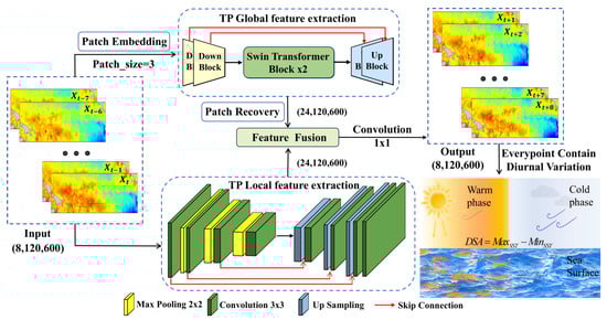
Figure 1. The Network CoTCN-DSV based on CoTCN to forecast diurnal SST variation (DSV).

The CoTCN consists of two parallel branches designed to capture complementary information. The first branch extracts large-scale (global) features using a Swin Transformer backbone, while the second branch focuses on fine-scale (local) features using a CNN-based U-Net. The first and second branches are called global branch and local branch, respectively. The outputs from the two branches are adaptively fused through a Squeeze-and-Excitation (SE) channel attention mechanism [31], followed by a 1 × 1 convolution to generate the final SST forecasts.

In the global branch, patch embedding was first applied using sliding 3 × 3 convolutions to divide the SST field into smaller patches. Two downsampling stages compressed the spatial dimensions, after which Swin Transformer [32] modules learnt long-range spatial dependencies. The features were then progressively upsampled, with skip connections restoring spatial details before patch recovery reconstructs the original spatial layout.

In the local branch, a CNN-based U-Net [33] structure was used. The encoder extracts local features through convolutional layers and pooling operations, while the decoder restores spatial resolution using upsampling layers and skip connections. The final convolution layer generates local SST features for forecasting.

A concise summary of the main architectural settings is provided in Table 1 to improve clarity for readers.

Table 1. Summary the key components of the CoTCN-DSV Architecture.

Parameters	Patch_Size	Embed_Dim	Window_Size	Dropout	UNet_Channels
Value	3	96	5	0.2	48

The SSTs from WHOI dataset have eight values at the 3 h intervals within a solar day. Therefore, each day contains the maximum and minimum SST values. To improve capturing SST extreme values (maximum and minimum), an Extreme Loss (EL) function was designed. Most existing forecast networks rely on the mean squared error (MSE) as the loss function, which tends to bias networks toward fitting smoothed mean states, thereby reducing their ability to represent extreme features in the diurnal cycle of SST. The proposed loss function extends the conventional MSE by incorporating additional terms associated with extreme values, thereby enhancing the network’s sensitivity to the maximum and minimum SST while preserving robust overall forecast performance.

$$Loss=L_{MSE}+{\alpha }_1{L}_{MAX}+{\alpha }_2{L}_{MIN}$$

(4)

$$L_{MSE}={\displaystyle \frac{1}{BTHW}}{\displaystyle \sum _{b=1}^B{\displaystyle \sum _{h=1}^H{\displaystyle \sum _{w=1}^W{\displaystyle \sum _{t=1}^T{(y_{b,t,h,w}-{\widehat{y}}_{b,t,h,w})}^2}}}}$$

(5)

$$L_{MAX}={\displaystyle \frac{1}{BHW}}{\displaystyle \sum _{b=1}^B{\displaystyle \sum _{h=1}^H{\displaystyle \sum _{w=1}^W{\displaystyle \sum _{t=1}^T{w}_{max,t}^{(b,h,w)}{(y_{b,t,h,w}-{\widehat{y}}_{b,t,h,w})}^2}}}}$$

(6)

$$L_{MIN}={\displaystyle \frac{1}{BHW}}{\displaystyle \sum _{b=1}^B{\displaystyle \sum _{h=1}^H{\displaystyle \sum _{w=1}^W{\displaystyle \sum _{t=1}^T{w}_{min,t}^{(b,h,w)}{(y_{b,t,h,w}-{\widehat{y}}_{b,t,h,w})}^2}}}}$$

(7)

$$w_{max,t}^{(b,h,w)}={\displaystyle \frac{e^{\beta y_{b,t,h,w}}}{{\displaystyle \sum _{t^{\prime }=1}^T{e}^{\beta y_{b,t^{\prime },h,w}}}}}$$

(8)

$$w_{min,t}^{(b,h,w)}={\displaystyle \frac{e^{-\beta y_{b,t,h,w}}}{{\displaystyle \sum _{t^{\prime }=1}^T{e}^{-\beta y_{b,t^{\prime },h,w}}}}}$$

(9)

where $B$ is Batch Size, $T$ is the length of the forecast sequence, and $H$ and $W$ represent the spatial dimensions. $y_{b,t,h,w}$ denotes the observed SST at batch b, time step t, and spatial location (h,w), while ${\widehat{y}}_{b,t,h,w}$ represents the corresponding SST forecast. $L_{MSE}$ is the global mean squared error that measures the overall prediction accuracy across all time steps and spatial locations, $L_{MAX}$ and $L_{MIN}$ are weighted error terms designed to emphasize prediction errors occurring near the temporal maximum and minimum SST states within each forecast sequence. The weighting mechanism is inspired by the Softmax function. In practice, this assigns relatively larger weights to time steps whose SST values are higher (for $L_{MAX}$) or lower (for $L_{MIN}$) compared to other time steps in the same sequence. As a result, errors associated with extreme SST states receive greater emphasis and contribute more strongly to gradient updates during network training. This design encourages the network to allocate more learning capacity to extreme SST conditions, which are often linked to important climate variability signals, while the global MSE term ensures stable overall prediction performance. Therefore, the loss function achieves a balance between global accuracy and extreme-event fidelity. Considering the exponential growth property of the exponential function, a scaling parameter $\beta$ was introduced to control the penalty strength for extreme values. Larger $\beta$ values produce sharper focus on the most extreme time steps. In addition, weighting coefficients ${\alpha }_1$ and ${\alpha }_2$ are used to balance the contributions of the maximum and minimum loss terms within the overall loss function. After extensive sensitivity experiments, the optimal parameter configuration ${\alpha }_1={\alpha }_2=4,\beta =5$ was selected.

All networks were trained under consistent experimental conditions on a platform equipped with eight DCU accelerators, which are optimized for deep learning workloads. The training was performed using the AdamW [34,35] optimizer. The initial learning rate was set to 0.001, with a weight decay coefficient of 0.1. The network was trained for 100 epochs with a batch size of 8.

2.4. Evaluation Indicators

To evaluate the forecasting skill of the model, this study employs the temporal correlation coefficient (R), spatial correlation coefficient (SCC), root mean square error (RMSE), mean absolute error (MAE), and bias as evaluation metrics. This study uses DSA to evaluate the intensity of DSV. These indicators are defined as follows:

$$R={\displaystyle \frac{{\displaystyle \sum _{t=1}^n}\left(y_t-\overline{y}\right)\left(y_t^{\prime }-\overline{y^{\prime }}\right)}{\sqrt{{\displaystyle \sum _{t=1}^n}{\left(y_t-\overline{y}\right)}^2}\sqrt{{\displaystyle \sum _{t=1}^n}{\left(y_t^{\prime }-\overline{y^{\prime }}\right)}^2}}}$$

(10)

$$SCC={\displaystyle \frac{{\displaystyle \sum _{i=1}^N}\left(O_{i,t}-\overline{O_t}\right)\left(O_{i,t}^{\prime }-\overline{O_t^{\prime }}\right)}{\sqrt{{\displaystyle \sum _{i=1}^N}{\left(O_{i,t}-\overline{O_t}\right)}^2}\sqrt{{\displaystyle \sum _{i=1}^N}{\left(O_{i,t}-\overline{O_t}\right)}^2}}}$$

(11)

$$RMSE=\sqrt{{\displaystyle \frac{1}{n}}{\displaystyle \sum _{t=1}^n}{\left(y_t-y_t^{\prime }\right)}^2}$$

(12)

$$MAE={\displaystyle \frac{1}{n}} |y_t^{\prime }-y_t|$$

(13)

$$Bias={\displaystyle \frac{1}{n}}{\displaystyle \sum _{t=1}^n}(y_t^{\prime }-y_t)$$

(14)

$$DSA=Ma{x}_{SST}-Mi{n}_{SST}$$

(15)

where $y_t$ is the referenced value at time t, $\overline{y}$ is the mean value corresponding to the referenced value, $y_t^{\prime }$ is the forecast value at time t, $\overline{y_t^{\prime }}$ is the mean value corresponding to the forecast value, and n is the total number of time series samples. $O_{i,t}$ denotes the referenced value at grid point i and time t, $O_{i,t}^{\prime }$ represents the forecast value, and $N$ is the total number of grid points. $Ma{x}_{SST}$ is the maximum SST within a solar day, and $Mi{n}_{SST}$ is represents the minimum SST within a solar day.

2.5. Experimental Design

In this study, we designed the following experiments. The first experiment uses the SST from WHOI dataset as the input. This was performed to examine the forecast skill of the CoTCN-DSV in diurnal SST variation over the equatorial Pacific. The second experiment was performed to examine the effect of revised loss functions on forecast performance. The third experiment was performed to test the effect of different input datasets on forecast result.

In the first experiment, the SST data from 1988 to 2010 were used for network training and validation, with data from 1988 to 2007 designated as the training set and data from 2008 to 2010 used as the validation set. The training set was employed to train the CoTCN-DSV, while the validation set was used to adjust the network and selected hyperparameters. SST data from 2011 to 2018 were reserved as an independent testing set. For each experiment, the network took SST data from eight consecutive time steps as input and produced SST forecasts for the subsequent eight time steps, which were evaluated against observed datasets for the same time.

After the training, the forecast performance of the daily maximum and minimum SST as well as the DSA was evaluated over the equatorial Pacific. Subsequently, to further investigate the forecast characteristics and regional differences associated with geographic location, three representative sites in the western, central, and eastern equatorial Pacific were selected for detailed analysis, namely the western Pacific site Pw (0.125°N, 140.125°E), the central Pacific site Pc (0.125°N, 162.875°W), and the eastern Pacific site Pe (0.125°N, 92.875°W). For these three sites, the climatological diurnal SST cycles and the probability distributions of DSA during 2011–2018 were analyzed. In addition, DSA during the year of 2016 which was marked by a rapid transition from strong El Niño to La Niña conditions, was analyzed to assess the robustness of the network’s DSV forecasts under extreme interannual climate variability.

In the second experiment, the effects of different data and the revised network with new loss function were compared to prove the advantages of the network.

In the third experiment, TAO buoy observations were also used to evaluate forecasted diurnal variation in SST derived from the WHOI-SST dataset over the testing period. Beyond acting as an independent validation benchmark, raw TAO time series were directly incorporated as network inputs to investigate the network’s sensitivity and generalization across different data sources. Furthermore, the performance of the network specifically trained using the TAO dataset was analyzed to quantify the potential improvement in forecast skill when high-fidelity physical observations are utilized.

3. Results

3.1. Forecasted SST and DSV

3.1.1. Forecasted Daily Maximum and Minimum SST

The maximum and minimum values of SST in a day are key phase characteristics of the diurnal cycle. Figure 2 presents the spatial distributions of the maximum and minimum SST between referenced (WHOI) and CoTCN-DSV forecasted values (Fc) at the lead time of 3 h (denoted as at the 3 h lead time) in the equatorial Pacific. The forecasted value at this lead time by CoTCN-DSV successfully reproduces the zonal and meridional thermal contrast, including the warming pool (>28 °C) in the western and cold tongue in the east, as well as the warm pool in the northeastern Pacific. This indicates that the network provides a reliable representation of the large-scale thermal structure in the tropical ocean. As shown in Figure 2e,f, at the first 3 h lead time, the RMSEs of both the maximum and minimum SSTs remain below 0.05 °C over most parts of the equatorial Pacific. Large errors (RMSE > 0.05 °C) are mainly confined to the eastern coastal regions, the cold tongue, and the coastal area off Peru both for the maximum and minimum SST forecasted by CoTCN-DSV.

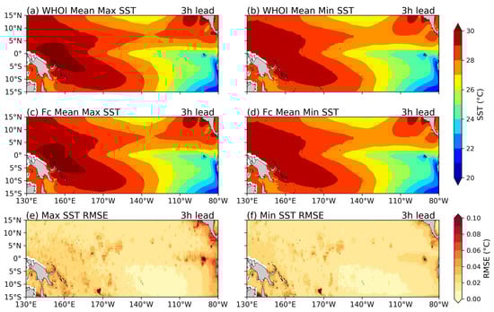
Figure 2. Time-averaged daily maximum and minimum SST from WHOI (a,b) and forecasted values (Fc) at the lead time of 3 h (denoted as at the 3 h lead time) by CoTCN-DSV (c,d). The RMSE values of the maximum (e) and minimum (f) values between WHOI and forecasted ones by CoTCN-DSV. The 2011–2018 data are used.

3.1.2. Forecasted DSA

Besides the maximum and minimum values, the amplitude of the diurnal SST cycle is a good index to quantify the intensity of DSV. In the following, the amplitude of the diurnal SST cycle forecasted by CoTCN-DSV is examined. At the 3 h lead time, the CoTCN-DSV exhibits good skill in forecasting DSA (Figure 3a–c). The forecasted DSA is highly consistent with that in WHOI with SCC reaching 0.99 at this lead time. Meanwhile, the averaged RMSE is less than 0.05 °C over the equatorial Pacific. Large DSA values (>0.4 °C) are primarily distributed in the western Pacific warm pool, the equatorial Pacific cold tongue, and the northeastern tropical Pacific warm pool. The large DSAs are basically located in the region of warm SST (Figure 2) except in the cold tongue. The RMSE of DSA is generally smaller than 0.1 °C compared with that in WHOI (Figure 3c). As with the distribution of large DSAs, large RMSEs are also located in the equatorial eastern Pacific, northeastern tropical Pacific warm pool and western Pacific warm pool. In the equator, the RMSE is larger in the eastern than that in the western Pacific. This spatial difference is likely related to the magnitude of DSA itself. The central Pacific is characterized by relatively weak diurnal SST variability, resulting in a smoother and more stable diurnal signal that may be easier for the model to learn and forecast.

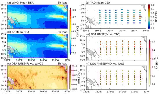
Figure 3. Time-averaged DSAs derived from the WHOI dataset (a), and forecasted DSA at 3 h lead time by CoTCN-DSV (b), and the RMSE between forecasted DSA at 3 h lead time by CoTCN-DSV and the WHOI DSA (c). Time-averaged DSA derived from TAO observations (d). RMSE of DSA between forecasted at 3 h lead time by CoTCN-DSV and TAO datasets (e), and between the WHOI and TAO datasets (f). The 2011–2018 data are used.

To validate forecasted DSA, the 10 min SST from buoy data from TAO are used. The observed DSA distribution is captured well by CoTCN-DSV (Figure 3d). The large DSAs (~0.5 °C) are also distributed in the western Pacific warm pool and the equatorial Pacific cold tongue. The low DSAs (<0.4 °C) are mainly located in the northwest and southwest corners in the study area. In TAO, the maximum DSA (>0.7 °C) occurs near the position at (0°, 95°W), which belongs to the Pacific cold tongue. In this region, rapid warming due to strong solar insolation daytime and strong cooling nighttime will induce the large DSA.

3.1.3. Forecasted DSA at Three Represented Positions

The forecasted and referenced DSVs present obvious spatial contrast, larger in the west and east, and smaller in the central on the equator. There are larger DSVs on the equator and small ones off the equator. To further investigate this spatial heterogeneity, three representative locations located in the western (Pw), central (Pc), and eastern (Pe) Pacific were selected for analysis. Figure 4 shows climatological mean forecasted DSVs for Pw, Pc and Pe at the 3 h lead time averaged over 2011–2018. The forecasted DSVs capture well the DSVs derived from WHOI data. Both in the forecasted and WHOI, the SST minimum values appear at 5:00–8:00 LT (Local Time), and the maximum values appear at 15:00–17:00 LT. The primary drivers of the diurnal variability of SST are solar radiation, wind forcing, and vertical mixing within the mixed layer. Although solar radiation reaches its maximum around local noon (12:00), the large heat capacity of the ocean causes a delayed thermal response, such that the SST maximum daytime typically occurs in the late afternoon (15:00–17:00 LT) [36]. After sunset, solar radiation vanished and the sea surface continuously loses heat through upward longwave radiation, and latent and sensible heat fluxes. This cooling destabilizes the water column, triggering convective mixing characterized by the sinking of colder surface water and the upward transport of warmer subsurface water, while wind stress further deepens the mixed layer. The nocturnal deepening of the mixed layer enhances surface cooling, leading to the minimum SST observed in the early morning hours (05:00–08:00 LT) [2].

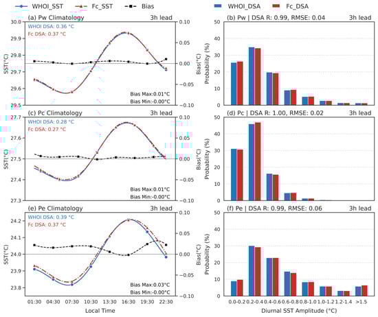
Figure 4. Climatological mean SST forecasts at the 3 h lead time for different locations (a,c,e) and the corresponding probability distributions of DSA (b,d,f). The 2011–2018 data are used.

In these three locations, the forecasted diurnal SST cycles match those from WHOI very well, respectively. The forecasted timings of the minimum and maximum SST for three locations are also consistent with those from WHOI. The forecasted maximum SST values are captured better than the forecasted minimum SST values at three locations, particularly at the Pe. At the Pe, the forecasted minimum value is larger than that from WHOI.

The forecasted climatological mean DSA values can capture the WHOI ones. In the WHOI, DSA are 0.36 °C, 0.28 °C and 0.39 °C at Pw, Pc and Pe, respectively. The forecasted DSA are 0.37 °C, 0.27 °C and 0.37 °C at Pw, Pc and Pe, respectively (Figure 4a,c,e). Among the three selected locations, Pe has the largest DSA error. Pc and Pw exhibit the smaller biases. At the Pe, the small, forecasted DSA is mainly due to the larger minimum value compared to that from WHOI.

At the 3 h lead time, the RMSE does not exceed 0.06 °C, and all the temporal correlation coefficients (Rs) exceed 0.99 at the three locations, indicating that the CoTCN-DSV network achieves very high forecast accuracy and reliability at short-term lead times. Notably, the RMSE at the central Pacific point Pc is only 0.02 °C, numerically lower than at Pw and Pe, indicating superior forecast performance at the central Pacific.

The probability density distributions of DSA (Figure 4b,d,f) can be used to estimate the underestimation or overestimation of the probability percentage at different DSA ranges. Most of the forecasted or referenced DSAs at Pw and Pc are primarily concentrated within the range of 0.0–0.4 °C, exceeding 50% and 70%, respectively. At Pe, forecasted or referenced DSAs within the range of 0.0–0.4 °C are less than 40%. At Pw, Pc and Pe relative to the WHOI, the forecasted DSAs are overestimated within the range of 0.0–0.2 °C, 0.2–0.4 °C and 0.0–0.2 °C, respectively.

At three points, when DSA values are greater than 0.8 °C, the probability percentage of forecasted DSA is overestimated. At the Pe, the forecast percentage exceeds the WHOI by 0.7% as the range > 1.5 °C. Therefore, the forecasted DSAs are slightly overestimated for large DSAs (>0.8 °C).

3.1.4. DSA Forecast as Different Lead Times

The above analysis primarily focused on forecast performance at the 3 h lead time. To further evaluate the network’s capability in capturing the diurnal cycle of SST, the DSA was further assessed across different lead times (Figure 5a–c).

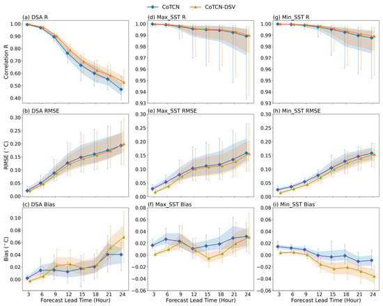
Figure 5. The effect of different loss functions on forecast metrics. R, RMSE and bias of DSA (a–c), daily maximum (d–f) and minimum (g–i) SST at different forecast lead times (from 3 h to 24 h). The CoTCN is trained using the mean squared error (MSE) loss, while the CoTCN-DSV is trained using the extreme loss (EL). The correlation coefficient R (a,d,g), RMSE (b,e,h), and Bias (c,f,i) are shown. The upper and lower error bars correspond to the 90th and 10th percentiles, while the shaded areas represent the interquartile range (75th–25th percentiles). The 2011–2018 data are used.

As the forecast lead time increases from 3 h to 24 h, forecast errors (RMSE, MAE, biases) increase and temporal correlation coefficients decrease. Forecasted RMSEs rise from 0.02 °C to 0.21 °C, MAEs increases from 0.01 °C to 0.15 °C, and R decreases from 0.99 to 0.53 (Table 2). As the lead times increase from 3 h to 24 h, CoTCN-DSV consistently maintains a high skill of DSA at all lead times. The median R (Figure 5a) remains above 0.5 at 24 h lead time, while the median RMSE (Figure 5b) is below 0.20 °C. At all lead times, CoTCN-DSV consistently maintains a very high skill for the maximum and minimum SST values. The median Rs are kept >0.98 and RMSEs are lower than 0.15 °C. The biases of the maximum/minimum SST value increase/decrease but are kept within 0.05 °C. These results demonstrate that the proposed network preserves reliable accuracy and consistency to forecast DSA.

Table 2. The median RMSE, MAE and R of DSA forecasted by the CoTCN-DSV network for the 2011–2018 test dataset.

Lead Times (h)	DSA RMSE (°C)	DSA MAE (°C)	DSA R
3	0.02	0.01	0.99
6	0.05	0.03	0.97
9	0.09	0.06	0.89
12	0.13	0.09	0.78
15	0.15	0.11	0.68
18	0.17	0.12	0.62
21	0.18	0.13	0.59
24	0.21	0.15	0.53

Feng et al. [26] applied an improved XGBoost model driven by wind speed and shortwave radiation in the equatorial Pacific region, obtaining an DSA RMSE of 0.23 °C and MAE of 0.16 °C. In contrast, the present network CoTCN-DSV achieves RMSE and MAE of 0.02 °C and 0.01 °C at the 3 h lead time, respectively. At the 24 h lead times, CoTCN-DSV can achieve RMSE and MAE of 0.21 °C and 0.15 °C. This indicates that the CoTCN-DSV has a good ability to forecast DSV and surpasses the XGBoost model which was built based on traditional machine learning even at the 24 h lead time. This can be attributed to the representation ability of nonlinear features.

3.1.5. Causes of DSA Forecast Errors

To further clarify where the DSA forecast errors mainly originate from, the errors of the forecasted maximum or minimum SST at the 24 h lead time are analyzed in detail. The distribution of time-averaged forecasted DSA exhibits highly spatial consistency with that of the DSA from WHOI (Figure 3a), with a SCC of 0.95. This is because the CoTCN-DSV network can capture the dominant spatial distributions of both the daily maximum and minimum SST at the 3 h lead time and at the 24 h lead time (Figure 6a,b).

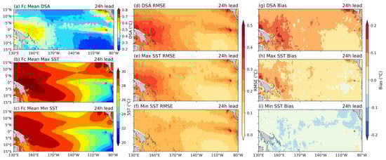
Figure 6. Spatial distributions of time-averaged forecasted DSA (a), daily maximum SST (b) and daily minimum SST (c), RMSE (d–f), and Bias (g–i) for DSA (a,d,g), daily maximum SST (b,e,h), and daily minimum SST (c,f,i) at the lead time of 24 h. The 2011–2018 data are used.

Spatially, the forecast error is smaller in the central equatorial region, than those in both the western and eastern equatorial regions. In the western Pacific warm pool region (130°E−170°W, 10°S–10°N), the RMSEs of DSA exceed 0.3 °C at the 24 h lead time. Correspondingly, substantial forecast errors in both the maximum and minimum SST are found in this region. In particular, the RMSEs of forecasted maximum SST generally reach 0.3–0.5 °C, whereas the RMSEs of forecasted minimum SST remain mostly within 0.1–0.2 °C. These results indicate that the DSA forecast errors in the western Pacific warm pool are primarily driven by insufficient representation of daytime warming in the afternoon, with errors in the maximum SST playing a dominant role. In the eastern Pacific cold tongue region (140°W–80°W, 5°S–5°N), the Peruvian coastal region, and the northeastern Pacific warm pool (120°W–80°W, 5°N–15°N), the RMSEs of both the maximum and minimum SST generally exceed 0.2 °C. Their combined contributions lead to relatively large DSA RMSEs in these regions. Further examination of the bias distribution shows that regions with large DSA RMSE values (>0.3 °C) are often accompanied by positive biases in forecasted maximum SST and negative biases in the forecasted minimum SST. This indicates that, at the 24 h lead time, the large RMSEs of DSA are mainly caused by the overestimation of the daily maximum SST and the underestimation of the daily minimum SST.

3.1.6. Forecasted DSA at Different Seasons in 2016

To examine the performance of CoTCN-DSV under strong events of interannual variability, this study focuses on the spatial distributions of forecasted RMSE of SST and DSA in 2016. According to the Oceanic Niño Index (ONI) released by NOAA/CPC, 2016 is a year characterized by a pronounced climate phase transition: the year began with the rapid decay of one of the strongest El Niño events on record, followed by a swift transition into a La Niña phase from mid-year to the latter half of the year. Such strong background-state provides an ideal testbed for evaluating the network’s forecasted performance under nonstationary climate conditions. To clearly characterize the seasonal evolution of forecasted errors, the forecasts at the 24 h lead time are analyzed for different seasons in 2016.

The forecasted RMSEs of DSA by CoTCN-DSV (Figure 7a–d) present seasonal variation associated with the distribution warm SST. From a spatial perspective, large forecast errors are primarily concentrated in three key regions: the Western Pacific Warm Pool (130°E–170°E, 10°S–10°N), the eastern Pacific cold tongue (120°W–80°W, 5°S–5°N), and the northeastern Pacific warm pool (110°W–80°W, 5°N–15°N). CoTCN-DSV has averaged RMSE values ranging from 0.216 °C to 0.23 °C throughout the year. The averaged SST RMSE also present seasonal variation (Figure 7e–h). By comparison, the seasonal variation in DSA RMSE is consistent with that of daily mean SST RMSE. The area-averaged SST RMSE consistently remains below 0.14 °C. The RMSE of daily mean SST at the 24 h lead time is within 0.12–0.15 °C. This forecast daily mean SST is pretty good as compared with previous studies by Zhang et al. [24,30,37]. These results indicate that the CoTCN-DSV achieves good daily mean SST and DSV across the entire equatorial Pacific. Even under conditions characterized by a rapid climate transition from El Niño to La Niña, the CoTCN-DSV demonstrates the strong generalization capability and forecast stability of SST and its diurnal cycle.

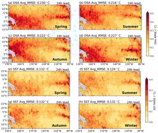
Figure 7. Spatial distributions of RMSE for DSA (a–d) and daily mean SST (e–h) across spring (a,e), summer (b,f), autumn (c,g), and winter (d,h) at the lead time of 8 h. The spring, summer, autumn, and winter represent March–May, June–August, September–November, and December–February, respectively. The 2016 data are used.

A detailed analysis was conducted for these regions with large RMSEs by examining the daily mean SST evolution and the corresponding daily DSA variations from March 2016 to February 2017 (Figure 8). Overall, across all three regions, the forecasted daily mean SST exhibits high consistency with that from WHOI in terms of phase evolution and oscillatory behavior, indicating that the CoTCN-DSV effectively captures the SST variation.

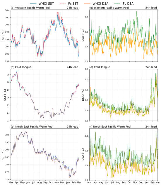
Figure 8. Seasonal variations in daily mean SST in 2016 (a,c,e) and DSA (b,d,f) in the Western Pacific Warm Pool (WP, 130°E–170°E, 10°S–10°N), the eastern Pacific cold tongue (CT, 120°W–80°W, 5°S–5°N), and the northeastern Pacific warm pool (NEP, 110°W–80°W, 5°N–15°N) at the lead time of 24 h. The WP (a,b), CT (c,d), and NEP (e,f) regions are shown. The 2016 data are used.

In the Western Pacific warm pool (WP) region (Figure 8a,b), SST remains above 29 °C throughout the year with relatively small variabilities. The fluctuations generally do not exceed 0.5 °C. During spring (March–May), SST shows a brief decline associated with the decay of the El Niño event, followed by a gradual increase driven by enhanced incoming solar shortwave radiation. In autumn (September–November), with the establishment of La Niña conditions, SST increases from approximately 29.1 °C in late August to 30.3 °C. During this period, the CoTCN-DSV slightly overestimates SST relative to that from WHOI, resulting in a seasonal mean SST RMSE of 0.253 °C—the highest among all seasons—while RMSE values in other seasons remain below 0.231 °C. Consistently, the forecast DSA RMSE in the WP region also increases markedly in autumn, with the RMSE of 0.351 °C, whereas values are below 0.314 °C in the other seasons. These results indicate that the CoTCN-DSV will overestimate diurnal variation under strong warming conditions in the warm pool.

In the eastern Pacific cold tongue (CT) region (Figure 8c,d), the forecasted daily mean SST variation captures that from WHOI well. This is because of the positive bias of the maximum SST and the negative bias of the minimum SST in a day in this region. The forecasted and WHOI SSTs undergo a pronounced rise followed by a rapid decline during spring, driven by the combined effects of the strong El Niño event and its subsequent rapid decay. Specifically, SST increases from approximately 28.3 °C in March to a peak of 29.5 °C in April, then sharply decreases to 23.5 °C by August within roughly four months. This intense thermodynamic adjustment substantially increases forecast difficulty, leading to the largest seasonal errors in this region, with springtime SST and DSA RMSE values reaching 0.242 °C and 0.322 °C, respectively.

In the northeastern Pacific warm pool (NEP) region (Figure 8e,f), the seasonal variability of DSA forecast errors is relatively small, with RMSE values ranging from 0.26 °C to 0.294 °C across the four seasons. In contrast, larger errors occur during spring (El Niño phase) and autumn (La Niña phase). SST RMSE reaches 0.213 °C during autumn, corresponding to multiple high-frequency oscillations in the SST time series between September and November (Figure 8e), during which the forecasted SST is generally slightly lower than that from WHOI.

Overall, despite the rapid transition between ENSO phases in 2016, the CoTCN-DSV maintains a robust capability to represent the evolution of SST and DSA across the equatorial Pacific. Nevertheless, forecast errors exhibit pronounced regional and seasonal dependence, with substantially larger errors occurring in the Western Pacific warm pool and eastern Pacific cold tongue during ENSO phase transitions, whereas forecast performance in the northeastern Pacific warm pool remains comparatively stable.

3.2. Effects of Improved Loss Functions

To assess the effectiveness of CoTCN-DSV by including the extreme loss (EL) and the forecasted DSA, the daily maximum and minimum SST are evaluated across all lead times using an independent testing dataset spanning 2011–2018.

As we know, CoTCN focused on global SST forecast and it employed a weighted loss function to account for spatial heterogeneity across different oceanic regions [30]. However, since the present study focuses on the equatorial Pacific, we chose the CoTCN trained with the MSE loss function as the baseline for comparison, ensuring a consistent and region-specific evaluation of the extreme loss.

Figure 5a–i provide the R, RMSE and bias of the forecasted DSA, and the daily maximum and minimum SST across different loss functions as a function of 3–24 h lead times. As the lead times increase from 3 h to 24 h, the CoTCN-DSV employing the EL consistently achieves larger R than that by the network using MSE-based loss function, daily maximum SST, and daily minimum SST forecasts. The reduction in RMSE achieved by the EL-based network relative to the MSE-based network persists across all lead times. As the lead time increases, the RMSEs by the CoTCN-DSV and CoTCN become closer. This behavior is likely attributable to the accumulation of forecast errors. The EL effectively mitigates the overestimation in the maximum SST forecasts, albeit with the side effect of introducing a slight underestimation for the minimum SST. It can be found that the DSA forecasted by the CoTCN-DSV exhibits a relatively large positive bias, slightly exceeding that of the MSE-based CoTCN at the 24 h lead time.

Quantification via regionally averaged RMSE confirms that the EL effectively enhances the forecast skill for the maximum and minimum SST in a day. Compared with the MSE-based CoTCN, the CoTCN-DSV reduces the forecasted time-averaged RMSEs of daily maximum SST by 10.9% at all lead times. From 3 h to 9 h, the RMSEs of daily maximum reduce by 38.1%, 27.1%, 5.1% by the CoTCN-DSV, respectively. For the daily minimum SST, time-averaged RMSEs reduce by 12.8%. From 3 h to 12 h, the RMSEs reduce by 42.1%, 20.5%, 17.7%, 10.0% by the CoTCN-DSV, respectively. These results demonstrate that incorporating EL effectively enhances the forecast skill of DSA and the daily maximum and minimum SST.

3.3. Effects of SST Data

To further assess the network’s capability in reproducing diurnal SST variation in a day, the forecast outputs were evaluated against TAO buoy observations (55 mooring sites) over the period 2011–2018. As the lead time increases from 3 h to 24 h (green curves in Figure 9), the median R between the forecast whose input is from WHOI SST and TAO observations decreases slightly from 0.951 to 0.946, while the median RMSE increases slightly from 0.323 °C to 0.343 °C. Meanwhile, the bias exhibits a persistently fluctuating positive offset. The mean R remains consistently above 0.93 at all lead times, this indicates strong spatiotemporal consistency. However, the relatively large initial mean RMSE (>0. 34 °C) and the sustained positive bias (>0.03 °C) suggest the possible presence of an inherent systematic discrepancy between the WHOI and TAO datasets.

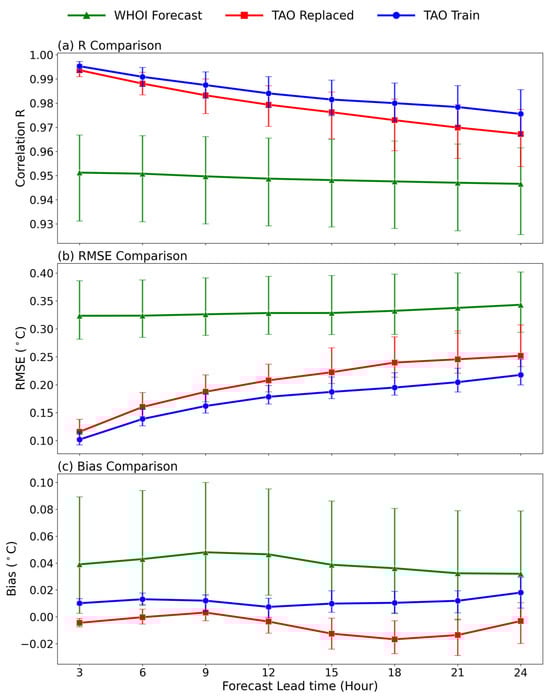
Figure 9. Against TAO buoy observations, evaluation metrics of forecasts 3 h SST whose forecast input employed WHOI-SST (green) and TAO data (red), and whose forecast and train inputs employed by TAO data (blue) compared with TAO buoy observations at the different lead times. The correlation coefficient R (a), RMSE (b), and Bias (c) are shown. The upper and lower error bars correspond to the 75th and 25th percentiles. The 2011–2018 data are used.

To determine whether these discrepancies originate from deficiencies in the CoTCN-DSV or from dataset-related biases, TAO buoy observations were directly fed into the CoTCN-DSV to generate forecasts but with no training using TAO data (red curves in Figure 9). Substantial improvements have been found across three evaluation metrics: the median R increases to 0.994, the median RMSE is reduced by approximately 64%, and the median bias is corrected from 0.040 °C to −0.004 °C at the 3 h lead time. In addition, the dispersion of these evaluation metrics is significantly narrowed, markedly enhancing the stability and consistency of the CoTCN-DSV. This comparison provides strong evidence that the previously forecast errors between WHOI and TAO primarily arise from systematic inconsistencies between datasets rather than deficiencies in the CoTCN-DSV, and also demonstrates the strong generalization capability of the CoTCN-DSV network across different data sources.

To examine the impact of data-source inconsistency on forecast performance, we further investigated whether unifying the training data can mitigate the bias. Specifically, since each TAO mooring is surrounded by four grid cells, the TAO observations were mapped back to these four collocated grid points using weights derived from inverse bilinear interpolation. These grid values in the training set were then replaced with the TAO-adjusted values, and the network was retrained accordingly (blue curves in Figure 9). The retrained network was then compared with forecasts generated by directly inputting TAO data (red curves). The results show clear improvements in both R and RMSE across all lead times, accompanied by a noticeable reduction in the dispersion of the evaluation metrics. In particular, the median R increases from 0.967 to 0.976, the median RMSE is reduced by approximately 13% at the 24 h lead time. Although the bias cannot be fully quantified by mean values due to positive–negative cancelation, the significantly narrowed interquartile range of the bias indicates a substantial reduction in systematic stability. This suggests that unifying data sources can effectively suppress the forecast errors.

Beyond high-frequency SST variation itself, the DSA performance of the CoTCN-DSV was further evaluated. Comparison of the forecasted DSA by the CoTCN-DSV using the WHOI SST at the 3 h lead time with TAO buoy observations (Figure 3e) reveals relatively large RMSE values at most buoy locations, with the largest errors concentrated in the eastern equatorial Pacific cold tongue. To determine whether these DSA discrepancies also stem from dataset-related biases, an additional comparison between WHOI-derived DSA and TAO-derived DSA was conducted. As shown in Figure 3e,f, the spatial distributions of RMSE are highly consistent between the two comparisons, with the largest errors consistently located in the cold tongue region. This further confirms that the apparent DSA forecast errors are largely attributable to systematic inconsistencies between the WHOI and TAO datasets rather than deficiencies in the forecast network (CoTCN-DSV) itself.

Finally, to verify the robustness and reliability of the CoTCN-DSV under different datasets, TAO buoy observations were incorporated into the WHOI-SST dataset at the corresponding grid points for network re-training, and the DSA forecast performance at the 3 h lead time was re-evaluated. The results indicate that for the CoTCN-DSV network trained with TAO data, the RMSE between the forecasted DSA and TAO-derived DSA is generally below 0.20 °C at most buoy locations, except for the eastern equatorial Pacific site at (0°, 95°W, Figure 10a).

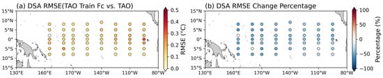
Figure 10. RMSE between forecasted DSA by the CoTCN-DSV that trained using TAO data and the derived DSA from TAO observations at the 3 h lead time (a). The percentage change in RMSE between forecasted DSA by the CoTCN-DSV (a) and that shown in Figure 3e (b). The 2011–2018 TAO data and WHOI data are used to test.

To further investigate the sources of error in simulating large-amplitude DSA, a diagnostic analysis was conducted at the (0°, 95°W) TAO mooring station. Given the absence of continuous shortwave radiation (SW) and mixed layer depth (MLD) observations at this site during 2011–2018, wind speed was utilized as the primary physical proxy to characterize the local air–sea conditions, owing to its dominant role in modulating surface mixing and MLD evolution. After rigorous quality control and temporal alignment, 2052 valid wind speed samples were obtained, yielding a long-term average of 5.33 m/s.

Figure 11 illustrates that while the network captures the overall seasonal cycle, it tends to overestimate DSA during extreme events (>0.87 °C), with a maximum positive bias of 2.92 °C. A representative extreme event on May 28, 2018, was selected for a detailed case study (Figure 12). During this event, the observed DSA reached 1.01 °C, while the forecasted DSA was 1.28 °C. The daily average wind speed was 3.36 m/s, which is 1.97 m/s lower than the long-term climatological mean of the station. Such distinct low-wind conditions suppress surface mixing in the upper ocean, serving as a key physical driver for the formation of this large DSA event [2]. High-resolution time-series analysis reveals that the forecast biases are not uniformly distributed throughout the day but are instead triggered by specific wind speed fluctuations. Specifically, between 13:30 and 16:30 LT, a sharp decline in wind speed (from 4.76 m/s to 3.58 m/s) coincided with a rapid divergence between the forecasted SST and the TAO observations. During this period of further weakened wind-driven mixing, the forecasted SST curve exhibited a significantly steeper gradient, reflecting that the network’s thermal response mechanism is highly sensitive to the transient weakening of vertical mixing. This led to a peak forecasted SST of 25.21 °C around 16:30 LT, notably higher than the observed 24.99 °C, resulting in an overestimated DSA of 1.28 °C. This case study partially explains the potential physical drivers of the network’s overestimation during extreme events, suggesting that the simulated response to surface heat accumulation may be too intense under transient low-wind scenarios.

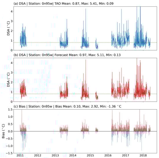
Figure 11. DSA derived from TAO observations at the (0°, 95°W) mooring during 2011–2018 (a). Forecasted DSA obtained from the network trained with TAO-substituted data (b). Bias between the forecasted DSA and the TAO-derived DSA (c).

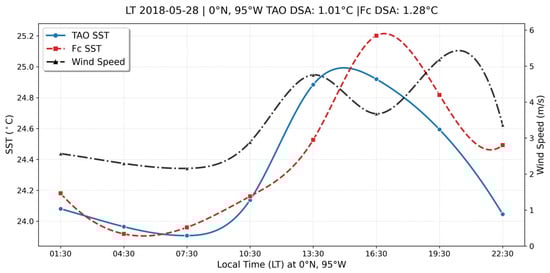
Figure 12. Variations in SST observed by TAO, forecasted SST (Fc SST), and wind speed at the (0°, 95°W) mooring on 28 May (LT).

Compared with the RMSE distribution obtained from the CoTCN-DSV trained by the WHOI dataset (Figure 3e), RMSEs are reduced at all grid points, with decreases ranging from 8% to 58% and an average reduction of 43% (Figure 10b). These results demonstrate that the CoTCN-DSV is suited for representing the diurnal variability of SST, and further confirm that the previously observed forecast errors primarily arise from systematic inconsistencies between datasets.

4. Conclusions

This study develops a DSV forecast network (CoTCN-DSV) based on the CoTCN and a revised loss function including the role of extremes to improve the forecast diurnal cycle of SST over the equatorial Pacific. This network is employed to forecast diurnal SST variation over the equatorial Pacific. At the 3 h lead time, the averaged RMSEs of both daily maximum and minimum SST are below 0.05 °C over most of the equatorial Pacific, indicating that the CoTCN-DSV effectively captures the spatial distribution of diurnal extremes. In addition, the overall forecast performance of the DSA is satisfactory, with a SCC of 0.99 between the time-averaged forecasted DSA and WHOI DSA, demonstrating strong spatial consistency. Across most regions, the DSA RMSE remains below 0.10 °C. Large DSAs from referenced data are well captured in the western Pacific warm pool, the equatorial Pacific cold tongue, and northeastern coastal regions, with TAO observations confirming accurate representation of extreme values. Additionally, the forecast skill over the central equatorial Pacific is higher than that over the western and eastern regions.

As the lead times increase, forecast errors gradually grow and correlations decrease. Nevertheless, even at the 24 h lead time, the CoTCN-DSV maintains high forecast accuracy, with RMSE below 0.21 °C and MAE below 0.16 °C. Overall, the model consistently outperforms traditional machine learning approaches, effectively capturing the nonlinear variability of SST and the spatiotemporal structure of DSA. At the larger lead time (e.g., 24h), The positive forecast bias in DSA is primarily caused by the overestimation of the daily maximum SST and the underestimation of the daily minimum SST.

For the year 2016, which experienced a rapid transition from El Niño to La Niña, the proposed model demonstrates robust generalization capability and forecast stability. At the 24 h lead time, the seasonal RMSE of DSA remains below 0.23 °C across all four seasons, while the corresponding daily mean SST RMSE maintains below 0.14 °C consistently. However, significant regional and seasonal differences in forecast errors are observed. In particular, errors increase markedly over the western Pacific warm pool and the eastern Pacific cold tongue during ENSO phase transitions, whereas forecast performance over the northeastern Pacific warm pool remains relatively stable.

Compared with the CoTCN using the conventional MSE loss, the CoTCN-DSV with improved loss shows improvements in forecasting daily maximum and minimum SST. Averaged across all lead times (24 h at the interval of 3 h), the averaged RMSE of daily maximum SST is reduced by 10.9%, and that of the daily minimum SST decreases by 12.8%, resulting in an overall enhancement of SST forecast skill. Moreover, the evaluation of high-frequency WHOI-SST and DSA forecasts against TAO observations further indicates that the relatively large forecast errors are primarily attributable to systematic discrepancies between the two datasets rather than deficiencies in the network architecture. When TAO data are directly incorporated into network training, the errors relative to TAO observations are markedly reduced, with an average reduction of 43%, further demonstrating the robustness of the network.

5. Discussion

This study focuses on DSV forecasting within a single-variable SST framework. Several directions may further improve DSV forecast performance in future work.

First, key factors influencing DSV, such as solar shortwave radiation, wind, and tidal currents could be incorporated as additional model inputs. Exploring appropriate data processing strategies will be investigated to enable the model to better capture diurnal variability and to learn the complex interactions among multiple variables, thereby achieving improved forecast skill.

Second, integrating dynamical model outputs with deep learning frameworks represents a crucial pathway to overcome the inherent limitations of single AI models, such as high data dependency and insufficient physical constraints. This integration can be implemented through two complementary strategies. On one hand, the outputs from ocean circulation models or air–sea coupled models can be incorporated as auxiliary input features or physical constraint conditions within the CoTCN-DSV architecture [38]. By leveraging the physical consistency of dynamical systems, such physics-informed AI approaches can effectively compensate for the lack of interpretability in purely data-driven models, thereby enhancing forecast robustness under complex or changing climate scenarios. On the other hand, a dedicated post-processing error correction system can be constructed by mining the spatiotemporal patterns of historical forecast errors. By analyzing error distributions across different lead times and regions—utilizing methods such as the “local dynamical analog”—targeted regression models can be developed to recalibrate the original CoTCN-DSV outputs [39,40]. Such hybrid schemes, which combine the powerful feature extraction of deep learning with the systematic bias reduction in post-processing, have demonstrated significant potential in SST forecasting studies. Implementing these integration strategies will likely further improve the physical consistency, stability, and reliability of DSV predictions.

It is also important to recognize the limitations associated with the current 3-hourly temporal sampling. Although 3-hourly data can resolve the overall structure of the diurnal cycle, SST peaks occurring on hourly or shorter timescales may be missed due to sampling frequency limitations, which may lead to underestimation of short-lived extremes, especially in regions with rapid SST changes. High-frequency observations from moored buoys or hourly satellite products can better resolve fine-scale temporal variations and provide valuable references for future model validation and improvement.

Future studies will further explore high-temporal-resolution reanalysis products and satellite observations, utilizing multi-source data fusion strategies to incorporate relevant physical variables and constraints from dynamical models. By bridging data-driven architectures with physical principles, we aim to achieve more accurate, robust, and physically consistent DSV forecasts.

References

- Sumner, M.D.; Michael, K.J.; Bradshaw, C.J.; Hindell, M.A. Remote Sensing of Southern Ocean Sea Surface Temperature: Implications for Marine Biophysical Models. Remote Sens. Environ. 2003, 84, 161–173. [Google Scholar] [CrossRef]
- Gentemann, C.L.; Donlon, C.J.; Stuart-Menteth, A.; Wentz, F.J. Diurnal Signals in Satellite Sea Surface Temperature Measurements. Geophys. Res. Lett. 2003, 30, 2002GL016291. [Google Scholar] [CrossRef]
- Steffen, J.; Seo, H.; Clayson, C.A.; Pei, S.; Shinoda, T. Impacts of Tidal Mixing on Diurnal and Intraseasonal Air-Sea Interactions in the Maritime Continent. Deep Sea Res. Part II Top. Stud. Oceanogr. 2023, 212, 105343. [Google Scholar] [CrossRef]
- Noh, Y.; Lee, E.; Kim, D.; Hong, S.; Kim, M.; Ou, M. Prediction of the Diurnal Warming of Sea Surface Temperature Using an Atmosphere-ocean Mixed Layer Coupled Model. J. Geophys. Res. 2011, 116, 2011JC006970. [Google Scholar] [CrossRef]
- Yang, X.; Bao, Y.; Song, Z.; Shu, Q.; Song, Y.; Wang, X.; Qiao, F. Key to ENSO Phase-Locking Simulation: Effects of Sea Surface Temperature Diurnal Amplitude. npj Clim. Atmos. Sci. 2023, 6, 159. [Google Scholar] [CrossRef]
- Kawai, Y.; Wada, A. Diurnal Sea Surface Temperature Variation and Its Impact on the Atmosphere and Ocean: A Review. J. Ocean. 2007, 63, 721–744. [Google Scholar] [CrossRef]
- Clayson, C.A.; Weitlich, D. Variability of Tropical Diurnal Sea Surface Temperature. J. Clim. 2007, 20, 334–352. [Google Scholar] [CrossRef]
- Zeng, X.; Beljaars, A. A Prognostic Scheme of Sea Surface Skin Temperature for Modeling and Data Assimilation. Geophys. Res. Lett. 2005, 32, 2005GL023030. [Google Scholar] [CrossRef]
- Takaya, Y.; Bidlot, J.; Beljaars, A.C.M.; Janssen, P.A.E.M. Refinements to a Prognostic Scheme of Skin Sea Surface Temperature. J. Geophys. Res. 2010, 115, 2009JC005985. [Google Scholar] [CrossRef]
- Zhang, H.; Beggs, H.; Merchant, C.J.; Wang, X.H.; Majewski, L.; Kiss, A.E.; Rodríguez, J.; Thorpe, L.; Gentemann, C.; Brunke, M. Comparison of SST Diurnal Variation Models Over the Tropical Warm Pool Region. JGR Ocean. 2018, 123, 3467–3488. [Google Scholar] [CrossRef]
- Weihs, R.R.; Bourassa, M.A. Modeled Diurnally Varying Sea Surface Temperatures and Their Influence on Surface Heat Fluxes. JGR Ocean. 2014, 119, 4101–4123. [Google Scholar] [CrossRef]
- Kantha, L.H.; Clayson, C.A. An Improved Mixed Layer Model for Geophysical Applications. J. Geophys. Res. 1994, 99, 25235–25266. [Google Scholar] [CrossRef]
- Karagali, I.; Høyer, J.L.; Donlon, C.J. Using a 1-D Model to Reproduce the Diurnal Variability of SST. JGR Ocean. 2017, 122, 2945–2959. [Google Scholar] [CrossRef]
- Börner, R.; Haerter, J.O.; Fiévet, R. DiuSST: A Conceptual Model of Diurnal Warm Layers for Idealized Atmospheric Simulations with Interactive Sea Surface Temperature. Geosci. Model Dev. 2025, 18, 1333–1356. [Google Scholar] [CrossRef]
- Breiman, L. Random Forests. Mach. Learn. 2001, 45, 5–32. [Google Scholar] [CrossRef]
- Cortes, C.; Vapnik, V. Support-Vector Networks. Mach. Learn. 1995, 20, 273–297. [Google Scholar] [CrossRef]
- LeCun, Y.; Bengio, Y.; Hinton, G. Deep Learning. Nature 2015, 521, 436–444. [Google Scholar] [CrossRef]
- Zhang, Z.; Pan, X.; Jiang, T.; Sui, B.; Liu, C.; Sun, W. Monthly and Quarterly Sea Surface Temperature Prediction Based on Gated Recurrent Unit Neural Network. J. Mar. Sci. Eng. 2020, 8, 249. [Google Scholar] [CrossRef]
- Taylor, J.; Feng, M. A Deep Learning Model for Forecasting Global Monthly Mean Sea Surface Temperature Anomalies. Front. Clim. 2022, 4, 932932. [Google Scholar] [CrossRef]
- Jia, X.; Ji, Q.; Han, L.; Liu, Y.; Han, G.; Lin, X. Prediction of Sea Surface Temperature in the East China Sea Based on LSTM Neural Network. Remote Sens. 2022, 14, 3300. [Google Scholar] [CrossRef]
- Zheng, G.; Li, X.; Zhang, R.-H.; Liu, B. Purely Satellite Data–Driven Deep Learning Forecast of Complicated Tropical Instability Waves. Sci. Adv. 2020, 6, eaba1482. [Google Scholar] [CrossRef] [PubMed]
- Xiao, C.; Chen, N.; Hu, C.; Wang, K.; Xu, Z.; Cai, Y.; Xu, L.; Chen, Z.; Gong, J. A Spatiotemporal Deep Learning Model for Sea Surface Temperature Field Prediction Using Time-Series Satellite Data. Environ. Model. Softw. 2019, 120, 104502. [Google Scholar] [CrossRef]
- Zhang, X.; Li, Y.; Frery, A.C.; Ren, P. Sea Surface Temperature Prediction with Memory Graph Convolutional Networks. IEEE Geosci. Remote Sens. Lett. 2021, 19, 8017105. [Google Scholar] [CrossRef]
- Zhang, T.; Lin, P.; Liu, H.; Wang, P.; Wang, Y.; Zheng, W.; Yu, Z.; Jiang, J.; Li, Y.; He, H. A New Transformer Network for Short-Term Global Sea Surface Temperature Forecasting: Importance of Eddies. Remote Sens. 2025, 17, 1507. [Google Scholar] [CrossRef]
- Von der Heydt, A.S.; Nnafie, A.; Dijkstra, H.A. Cold Tongue/Warm Pool and ENSO Dynamics in the Pliocene. Clim. Past 2011, 7, 903–915. [Google Scholar] [CrossRef]
- Feng, Y.; Gao, Z.; Xiao, H.; Yang, X.; Song, Z. Predicting the Tropical Sea Surface Temperature Diurnal Cycle Amplitude Using an Improved XGBoost Algorithm. J. Mar. Sci. Eng. 2022, 10, 1686. [Google Scholar] [CrossRef]
- Kawai, Y.; Kawamura, H. Evaluation of the Diurnal Warming of Sea Surface Temperature Using Satellite-Derived Marine Meteorological Data. J. Oceanogr. 2002, 58, 805–814. [Google Scholar] [CrossRef]
- Moody, J.; Darken, C.J. Fast Learning in Networks of Locally-Tuned Processing Units. Neural Comput. 1989, 1, 281–294. [Google Scholar] [CrossRef]
- Wolpert, D.H. Stacked Generalization. Neural Netw. 1992, 5, 241–259. [Google Scholar] [CrossRef]
- Zhang, T.; Lin, P.; Liu, H.; Wang, P.; Wang, Y.; Xu, K.; Zheng, W.; Li, Y.; Jiang, J.; Zhao, L. A Coupled Transformer-CNN Network: Advancing Sea Surface Temperature Forecast Accuracy. IEEE Trans. Geosci. Remote Sens. 2025, 63, 4207414. [Google Scholar] [CrossRef]
- Hu, J.; Shen, L.; Sun, G. Squeeze-and-Excitation Networks. In Proceedings of the IEEE Conference on Computer Vision and Pattern Recognition, Salt Lake City, UT, USA, 18–23 June 2018; IEEE Computer Society: Washington, DC, USA, 2018; pp. 7132–7141. [Google Scholar]
- Liu, Z.; Lin, Y.; Cao, Y.; Hu, H.; Wei, Y.; Zhang, Z.; Lin, S.; Guo, B. Swin Transformer: Hierarchical Vision Transformer Using Shifted Windows. In Proceedings of the IEEE/CVF International Conference on Computer Vision, Montreal, BC, Canada, 11–17 October 2021; pp. 10012–10022. [Google Scholar]
- Çiçek, Ö.; Abdulkadir, A.; Lienkamp, S.S.; Brox, T.; Ronneberger, O. 3D U-Net: Learning Dense Volumetric Segmentation from Sparse Annotation. In Medical Image Computing and Computer-Assisted Intervention—MICCAI 2016; Ourselin, S., Joskowicz, L., Sabuncu, M.R., Unal, G., Wells, W., Eds.; Lecture Notes in Computer Science; Springer International Publishing: Cham, Switzerland, 2016; Volume 9901, pp. 424–432. ISBN 978-3-319-46722-1. [Google Scholar]
- Kingma, D.P. Adam: A Method for Stochastic Optimization. arXiv 2014, arXiv:1412.6980. [Google Scholar]
- Loshchilov, I.; Hutter, F. Decoupled Weight Decay Regularization. arXiv 2017, arXiv:1509.03545. [Google Scholar] [CrossRef]
- Tu, Q.; Hao, Z.; Liu, D.; Tao, B.; Shi, L.; Yan, Y. The Impact of Diurnal Variability of Sea Surface Temperature on Air–Sea Heat Flux Estimation over the Northwest Pacific Ocean. Remote Sens. 2024, 16, 628. [Google Scholar] [CrossRef]
- Zhang, T.; Lin, P.; Liu, H.; Zheng, W.; Wang, P.; Xu, T.; Li, Y.; Liu, J.; Chen, C. Short-Term Sea Surface Temperature Forecasts for the Equatorial Pacific Based on Long Short-Term Memory Network. Chin. J. Atmos. Sci. 2024, 48, 745–754. [Google Scholar]
- Ham, Y.-G.; Kim, J.-H.; Luo, J.-J. Deep Learning for Multi-Year ENSO Forecasts. Nature 2019, 573, 568–572. [Google Scholar] [CrossRef]
- Hou, Z.; Zuo, B.; Zhang, S.; Huang, F.; Ding, R.; Duan, W.; Li, J. Model Forecast Error Correction Based on the Local Dynamical Analog Method: An Example Application to the ENSO Forecast by an Intermediate Coupled Model. Geophys. Res. Lett. 2020, 47, e2020GL088986. [Google Scholar] [CrossRef]
- Hou, Z.; Li, J.; Zuo, B. Correction of Monthly SST Forecasts in CFSv2 Using the Local Dynamical Analog Method. Weather Forecast. 2021, 36, 843–858. [Google Scholar] [CrossRef]
Disclaimer/Publisher’s Note: The statements, opinions and data contained in all publications are solely those of the individual author(s) and contributor(s) and not of MDPI and/or the editor(s). MDPI and/or the editor(s) disclaim responsibility for any injury to people or property resulting from any ideas, methods, instructions or products referred to in the content. |
© 2026 by the authors. Licensee MDPI, Basel, Switzerland. This article is an open access article distributed under the terms and conditions of the Creative Commons Attribution (CC BY) license.