Mapping Soil Trace Metals Using VIS–NIR–SWIR Spectroscopy and Machine Learning in Aligudarz District, Western Iran

Highlights

What are the main findings?

• VIS–NIR–SWIR spectroscopy combined with ML (ANNs, SVR) accurately predicts soil Cr, As, Cu, and Cd.
• Predicted spatial patterns match key geological features of the Sanandaj–Sirjan Zone (western Iran).

What are the implications of the main findings?

• Provides a fast, non-destructive, and scalable alternative to laboratory geochemical assays.
• The workflow can be transferable to airborne and satellite hyperspectral missions for large-area soil metal mapping.

Abstract

Detecting trace metals in soil across geologically diverse terrains remains challenging due to complex mineral–metal interactions and the limited spatial coverage of traditional geochemical tests. This study develops a scalable VIS–NIR–SWIR spectroscopy and machine learning (ML) framework to predict and map soil concentrations of Cr, As, Cu, and Cd in the Aligudarz District, located within the geotectonically complex Sanandaj–Sirjan Zone of western Iran. Laboratory reflectance spectra (~350–2500 nm) obtained from 110 soil samples were pre-processed using derivative filtering, scatter-correction techniques, and genetic algorithm (GA)-based wavelength optimisation to enhance diagnostic absorption features linked to Fe-oxides, clay minerals, and carbonates. Multiple ML-based approaches, including artificial neural networks (ANNs), support vector regression (SVR), and partial least squares regression (PLSR), as well as stepwise multiple linear regression (SMLR), were compared using nested, spatial, and external validation. Nonlinear models, particularly ANNs, exhibited the highest predictive accuracy, with strong generalisation confirmed via an independent test set. GA-selected wavelengths and derivative-enhanced spectra revealed mineralogical controls on metal retention, confirming that spectral predictions reflect underlying geological processes. Ordinary kriging of spectral-ML residuals generated spatially consistent metal-distribution maps that aligned well with local and regional geological features. The integrated framework demonstrates high predictive accuracy and operational scalability, providing a reproducible, field-ready method for rapid geochemical assessment. The findings highlight the potential of VIS–NIR–SWIR spectroscopy, combined with advanced modelling and geostatistics, to support environmental monitoring, mineral exploration, and risk assessment in geologically complex terrains.

1. Introduction

Soil-borne trace metals, including chromium (Cr), copper (Cu), arsenic (As), and cadmium (Cd), have a significant impact on environmental quality, ecosystem stability, and human health [1,2,3,4]. Their mobility, bioavailability, and ecological effects are influenced by complex interactions among mineralogical composition, redox conditions, and sorption–desorption processes. Conventional laboratory-based geochemical methods, such as inductively coupled plasma mass spectrometry (ICP-MS) and X-ray fluorescence (XRF), offer precise quantitative measurements but are inherently destructive, costly, and limited in spatial coverage, restricting their usefulness for large-scale environmental monitoring and prompt risk assessment [5,6,7].

Reflectance spectroscopy across the visible, near-infrared, and shortwave infrared (VIS–NIR–SWIR; ~400–2500 nm) spectral ranges has thus become a fast, non-invasive, and scalable remote sensing method for characterising soil mineralogy and related geochemical properties [8,9,10,11,12]. The physical basis of VIS–NIR–SWIR spectroscopy lies in electronic transitions and molecular vibrational processes that give rise to diagnostic absorption features linked to specific mineral components. In soils, Fe-oxides and hydroxides (e.g., hematite and goethite) dominate spectral behaviour in the VIS–NIR region via crystal-field electronic transitions, resulting in broad absorptions between ~400 and 550 nm and distinctive reflectance shifts across the red/near-infrared boundary [13]. Conversely, clay minerals and carbonates mainly influence the SWIR region, where overtone and combination absorptions of OH⁻ and CO₃²⁻ molecular bonds produce diagnostic features near ~1400 and ~1900 nm, as well as near ~2200–2250 nm for Al–OH–bearing phyllosilicates and around ~2300–2350 nm for carbonate minerals [14]. In addition, moisture content decreases reflectance across the entire spectrum, with a more pronounced effect on specific absorption features near 1400 nm and 1900 nm, as well as throughout the SWIR region [15]. These absorption mechanisms and their mineralogical relevance are well understood in rock and mineral spectroscopy and underpin soil spectral interpretation within the VIS–NIR–SWIR domain [8,9].

When combined with appropriate calibration and modelling strategies, VIS–NIR–SWIR spectroscopy enables indirect estimation of trace-metal concentrations in soils, plants, and rocks, offering strong potential for environmental monitoring and mineral exploration [16,17,18,19,20,21,22,23]. However, most trace metals do not exhibit unique or directly observable absorption features within the VIS–NIR–SWIR range. Their spectral detectability therefore depends largely on indirect mineralogical proxies, such as Fe-oxides, hydroxides, and phyllosilicates, which govern metal retention, adsorption, and co-precipitation processes in soils [24,25]. This indirect spectral–geochemical relationship requires analytical frameworks that prioritise robust spectral pre-processing to enhance subtle diagnostic features, transparent and reproducible feature-selection strategies, and modelling approaches capable of capturing high-dimensional and nonlinear relationships between spectral responses and geochemical variables [23,24,25,26]. Recent studies have shown that derivative-based spectral transformations and targeted wavelength selection can substantially improve model stability, predictive accuracy, and physical interpretability [27,28,29].

Over the past decade, the integration of VIS–NIR–SWIR spectroscopy with machine learning (ML) techniques has become increasingly common for soil geochemical characterisation and for assessing mining-related contamination, demonstrating strong potential for predicting the levels of potentially toxic elements in various environments [30,31,32]. At the same time, notable progress has been made in mineral exploration, including mapping Cu mineralisation, identifying hazardous mineral fibres, and detecting regional hydrothermal alteration zones [23,33,34,35]. Despite these advances, several methodological challenges still exist. Many studies rely on single-model workflows, which limit systematic comparisons of spectral pre-processing, feature selection, and modelling approaches, thereby reducing reproducibility [36,37,38,39,40,41]. Model validation often remains limited to internal k-fold cross-validation, with infrequent use of independent test sets, nested validation, and spatial or block-based cross-validation, leading to overly optimistic accuracy estimates and limited robustness assessment [42,43]. Moreover, spectroscopic predictions are often presented without sufficient geological context, which diminishes their interpretability and operational usefulness for environmental monitoring and mineral exploration [42,43,44,45]. As a result, issues related to reproducibility, transferability, and uncertainty quantification are still widely acknowledged in the remote sensing literature (e.g., [16,19,46]).

To address these limitations, this study develops an integrated and reproducible framework that combines VIS–NIR–SWIR spectroscopy, ML, and geostatistics to predict and map soil trace-metal concentrations. The methodological innovation involves systematically evaluating spectral pre-processing techniques, using genetic algorithms (GA) to optimise wavelength selection, and comparing both linear and nonlinear modelling strategies within a unified workflow. Modelling performance and robustness are assessed using nested, spatial/block, and external validation strategies, and the results are interpreted within a clear geological and mineralogical context. By explicitly linking spectral–ML predictions to lithological and structural controls and integrating them with geostatistical interpolation, the framework produces spatially consistent and physically interpretable maps of trace-metal distribution.

The framework is applied to the Aligudarz District in Lorestan Province, western Iran, situated within the Sanandaj–Sirjan zone of the Zagros orogenic belt. This region is characterised by a complex tectono-magmatic history involving magmatism, metamorphism, sedimentation, active faulting, and hydrothermal alteration, leading to significant spatial heterogeneity and enrichment of Cr, As, Cu, and Cd [47,48,49]. Hydro-climatic variability further influences trace-metal mobility, particularly Cr in ultramafic-hosted terrains [50,51], making the area a challenging yet representative natural laboratory for testing predictive geochemical mapping approaches under heterogeneous geological conditions.

Accordingly, the objectives of this study are: (1) to develop a reproducible VIS–NIR–SWIR spectroscopy-ML modelling workflow for predicting soil Cr, As, Cu, and Cd concentrations; (2) to systematically evaluate the impact of spectral pre-processing, feature selection, and modelling strategy on predictive performance; (3) to assess the robustness and generalisation of modelling outcomes using nested, spatial/block, and external validation schemes; and (4) to integrate spectral–ML predictions with geostatistical interpolation and geological information to produce spatially continuous and interpretable soil trace-metal maps relevant to environmental monitoring, public health risk assessment, and mineral exploration.

2. Regional Setting and Study Area

The study area is in the Aligudarz District of Lorestan Province, western Iran, within 49°40′08′′–49°41′10′′E and 33°25′47′′–33°26′38′′N (Figure 1). The landscape features rugged mountains that rise to more than 2000 m. The average annual precipitation varies from 450 to 800 mm in a temperate montane climate, resulting in distinct weathering regimes that notably influence soil mineralogy and geochemistry [52].

Shaped by long-term tectono-magmatic geological processes, the district lies within the Sanandaj–Sirjan Zone (SSZ) of the Zagros orogen, a primary tectono-magmatic belt formed through successive phases of convergence and continental collision between the Arabian and Eurasian plates [47,49,53]. This evolution has produced a heterogeneous assemblage of Palaeozoic–Cenozoic igneous, metamorphic, and sedimentary units, extensive fault networks, and chemically variable alteration zones, creating complex spatial patterns in the near-surface geochemistry. Thus, the region contains extensive intrusive and volcanic rocks, including basalts, andesites, diorites, and granitic bodies, that record multiple episodes of emplacement and deformation. Hydrothermal alteration linked to these units has enhanced Cu–Cr enrichment through magmatic differentiation and fluid-mediated remobilisation [54]. Iron-rich minerals such as magnetite and hematite are abundant and exhibit distinctive VIS–NIR–SWIR spectral features that aid in predicting Cu and Cr. Metamorphic rocks, including schists, amphibolites, and gneisses, reflect high-temperature, high-pressure tectono-thermal events within the SSZ [55]. Contact metamorphism between intrusions and carbonate hosts has generated skarn-type Cu–Cr systems [56]. These metamorphic units contain chlorite, epidote, and amphibole, adding to spectral diversity in the SWIR region and providing a valuable test of spectral modelling generalisation. Jurassic–Neogene sedimentary successions, comprising sandstone, limestone, and shale, are widespread. Carbonate and shale units may host As and Cd, mobilised through weathering and leaching processes [48]. These lithologies induce subtle spectral variations related to carbonate absorption and clay content, further increasing the heterogeneity of the geochemical landscape.

Figure 1. The regional geographic location of the study area, the corresponding geological map [47,49,57], and the spatial distribution of the 110 soil samples collected are shown.

Figure 1. The regional geographic location of the study area, the corresponding geological map [47,49,57], and the spatial distribution of the 110 soil samples collected are shown.

Beyond its geological complexity, the SSZ is recognised as one of Iran’s most important metallogenic belts, hosting numerous mineral deposits and small-scale mining operations related to Cu, Fe, Cr, and associated trace elements [47,49]. In the study area, mineralisations are primarily structurally controlled and linked to intrusive activity, alteration zones, and fault-guided fluid pathways. Although large-scale industrial mining remains limited, historical and artisanal extraction, along with documented mineral prospects, indicate a long-standing interaction between mineralised bedrock and surface environments. From an environmental perspective, this context is vital: elevated soil concentrations of trace metals may reflect natural geogenic enrichment rather than direct human activities, yet they still pose potential ecological and human health risks when mobilised into soils, waters, and food chains. This issue is particularly relevant in the context of Iran’s strategic objectives to expand and modernise its mining sector, which includes increasing mineral production and developing exploration and extraction activities in resource-rich regions such as the Aligudarz District.

The regional active compressional tectonic regime promotes the movement of hydrothermal fluids through fractures, leading to structurally controlled enrichments of Cu, Cr, and As [47,49]. These features create significant spatial anisotropy in trace-metal distributions and induce spectral overprinting, facilitating a detailed assessment of geological sensitivity in spectral modelling.

3. Materials and Methods

Figure 2 shows the main methodological stages and procedures of this investigation, highlighting (1) field sampling and laboratory analysis, (2) spectral data processing, (3) model-building strategies, and (4) geostatistical integration and mapping.

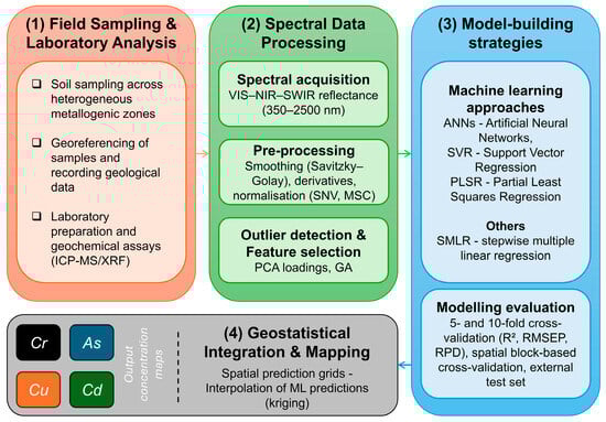
Figure 2. Methodological flowchart used in this work (more details in the text).

All used analytical techniques, processing procedures, modelling parameters, and spatial integration approaches were predefined to ensure reproducibility and prevent post hoc adjustments [58,59,60].

3.1. Field Sampling and Laboratory Analysis

The sampling strategy was developed through a geological assessment of the study area. A regional 1:100,000-scale geological map was examined to characterise the spatial lithostratigraphic variability and the structural controls related to the SSZ [47,49,57] (Figure 1). Additional insights from more recent structural and metallogenic studies have further enhanced the understanding of the interactions among deformations, intrusive activity, and hydrothermal processes in shaping the near-surface geochemical patterns of the study area [61,62].

In the field, 110 soil samples were collected across the study area as composite samples from the continuous 10–20 cm depth interval. Material was extracted throughout the entire interval and homogenised to reduce the influence of transient surface contamination and organic inputs, while capturing the geochemically active sub-surface soil horizon. This depth range was selected to ensure consistency among samples and to represent soil layers most relevant to weathering processes, trace-metal mobility, and surface–subsurface geochemical interactions (e.g., [7]). Sampling locations were selected using a stratified random design, in which the study area was first divided into spatial domains defined by lithostratigraphic units, major structural features, and hydrothermal alteration (metallogenic) zones. Within each sampling domain, locations were randomly assigned to ensure unbiased spatial coverage while maintaining geological representativeness. This method aimed to capture both regional- and local-scale variability related to lithology, structure, and alteration intensity. All samples were georeferenced, and lithological attributes along with structural context were recorded during fieldwork to support the interpretation of the predictive geochemical maps.

Concentrations of Cr, Cu, As, and Cd were measured at the Geological Survey of Iran, Central Laboratory, in Tehran. Before analysis, soil samples were oven-dried at 40–45 °C, homogenised, sieved through a 2-mm nylon mesh, and then ground to less than 75 μm using an agate mill to prevent metal contamination. For ICP–MS analysis, approximately 0.5 g of homogenised soil sample was digested with a multi-acid protocol (HF–HNO₃–HClO₄) in a closed-vessel microwave digestion system (Milestone Ethos UP, Sorisole, Italy). Major and trace element concentrations were analysed using an Agilent 7900 ICP–MS (Santa Clara, CA, USA), following internationally recognised protocols for soil geochemistry. Sample preparation, digestion, calibration, and quality control procedures adhered to U.S. Environmental Protection Agency (EPA) methods for total metal determination in soils (e.g., EPA Method 3052) and relevant ISO standards for elemental analysis in solid matrices (e.g., ISO 17294-2 and ISO 11466). Detection limits for the instruments typically were Cr < 0.2 mg/kg, Cu < 0.1 mg/kg, As < 0.05 mg/kg, and Cd < 0.01 mg/kg. Analytical precision, evaluated through repeated measurements of certified reference materials (NIST 2711a, GBW 07405), was generally better than 5%. To independently verify the ICP–MS results and ensure inter-instrument consistency, X-ray fluorescence analyses were performed using a PANalytical Axios FAST wavelength-dispersive XRF (WD-XRF) spectrometer (Malvern Panalytical, Almelo, The Netherlands) (see https://www.malvernpanalytical.com/en/products/product-range/axios-fast (accessed on 10 January 2026)), operated under vacuum conditions on pressed powder pellets. The XRF analytical uncertainty for the target elements was less than 3%. Quality assurance and quality control included instrument calibration with multi-element standards, procedural blanks, laboratory duplicates (10% of all samples), and certified reference materials to guarantee accuracy and reproducibility of the geochemical dataset.

After data acquisition, geochemical raw data were subjected to statistical analysis, including Pearson’s correlation to elucidate relationships among elements within the dataset [63,64], and a one-way analysis of variance (ANOVA) (see https://www.sciencedirect.com/topics/psychology/analysis-of-variance (accessed on 10 January 2026)) to assess spatial variation across data subsets [65,66,67].

3.2. Spectral Data Processing

VIS–NIR–SWIR reflectance spectra were acquired in the laboratory using an ASD FieldSpec^® 3 spectroradiometer (Analytical Spectral Devices, Boulder, CO, USA; see www.asdi.com), covering the spectral range of ~350–2500 nm. Measurements were performed under consistent lighting conditions and free from atmospheric interference. Prior to each measurement, the instrument was calibrated using a Spectralon white reference panel (Labsphere, Inc., North Sutton, NH, USA) to ensure radiometric accuracy. A uniform spectral geometry was maintained with a probe height of approximately 30 cm and an illumination incidence angle of 30°, using a fixed measurement stand to ensure consistency across samples. Each sample was scanned three times, and the average spectrum was calculated after discarding any spurious or noisy scans [21,68]. Although the mid-infrared (MIR) region beyond 2500 nm was inaccessible, the SWIR range encompasses many diagnostic overtones and combination bands related to Fe-oxides, hydroxyl-bearing minerals, and clay structures, which are key indicators of trace-metal adsorption mechanisms in soils [69,70,71].

Mineralogical interpretation and spectral identification were supported by reference spectral libraries, including the ASTER Spectral Library Version 2.0 [72] and the USGS Spectral Library Version 7 [73]. These library spectra were supplemented by in-house measurements of pure mineral standards under controlled laboratory conditions. All reference spectra were acquired at the same resolution as the sample measurements (3 nm in the VIS–NIR, 10 nm in the SWIR).

Spectral pre-processing aimed to reduce noise, correct scattering effects, and enhance diagnostic absorption features while preserving spectral interpretability. Raw spectra were trimmed to 400–2450 nm to remove detector-edge noise and spectral overlap artefacts [74,75], then smoothed using a Savitzky–Golay filter (window size = 11, polynomial order = 2) [58]. First- and second-derivative transformations were applied to highlight broad, overlapping absorption bands typically associated with Fe-oxide and clay minerals [32,76]. Baseline offsets and scattering due to grain-size heterogeneity were corrected using standard normal variate and multiplicative scatter correction sequentially [77,78], improving visibility of subtle features critical for indirect geochemical modelling [79,80]. For interpretative and visualisation purposes, selected spectra were also expressed in absorbance units, calculated as A = log₁₀(1/R), where R is reflectance. While reflectance is the conventional representation for mineral spectral signatures, absorbance representation enhances subtle absorption features by linearising weak spectral responses and reducing continuum effects, particularly in the VIS and NIR regions. This transformation is widely used in derivative-based spectral analysis and chemometric applications to improve the identification of overlapping absorption bands associated with Fe-oxides, clay minerals, and other indirect mineralogical proxies relevant to trace-metal retention. Importantly, absorbance was derived directly from reflectance measurements and does not alter the underlying spectral information used for modelling.

Outlier spectra were identified using Mahalanobis distance analysis within the principal component analysis (PCA) space [81]. PCA was also employed to characterise major variance components and to facilitate reproducible calibration–validation partitioning [82], serving as a quality-control step for internal spectral consistency.

Feature selection for predicting soil concentrations of Cr, Cu, As, and Cd was performed using a genetic algorithm (GA) [36,83]. GA parameters included a population size of 100, crossover probability of 0.8, mutation rate of 0.05, 100 generations, and 5-fold RMSE cross-validation as the fitness criterion, balancing exploration and convergence while reducing overfitting risk [28,84]. Only the GA-selected wavelength subsets were used as inputs for spectral modelling.

3.3. Model-Building Strategies

Spectral ML-based modelling was conducted using artificial neural networks (ANNs), support vector regression (SVR), and partial least squares regression (PLSR) approaches. ANNs offer nonlinear, multilayer computational frameworks capable of learning complex relationships between spectral variables and geochemical concentrations [85,86,87]. The ANN architecture used was a two-layer feedforward network with 64 and 32 neurons, respectively, and ReLU activations. ANN training employed the Adam optimiser (learning rate = 0.001; batch size = 16), with early stopping to prevent overfitting. SVR, based on statistical learning theory, utilises kernel functions to transform high-dimensional spectral features into an optimised regression space while balancing model complexity [88,89]. SVR was implemented with a radial basis function kernel, and optimal hyperparameters (C = 10, γ = 0.01, ε = 0.1) were identified using 5-fold cross-validation with a grid search. PLSR, a commonly used latent-variable method, reduces spectral collinearity by projecting predictors onto orthogonal components that maximise covariance with the response [90,91]. PLSR employed the NIPALS algorithm [92], selecting 15 latent variables based on the lowest cross-validated RMSE.

To provide a transparent statistical benchmark, stepwise multiple linear regression (SMLR) was also utilised. Although not an ML technique, SMLR provides a clear linear comparison with nonlinear approaches [93]. It iteratively selects significant predictors using information-theoretical criteria, providing a complementary linear baseline [83]. SMLR was implemented using an AIC-based forward–backward procedure as described in [94,95].

All models were trained using identical data partitions to enable fair comparison. The dataset of 110 samples was divided into a calibration subset (85 samples; 77%) and an internal validation subset (25 samples; 23%) using stratified random sampling to preserve the distribution of element concentrations.

Modelling evaluation followed a multi-stage protocol aligned with best-practice guidelines for predictive modelling [96,97]. Nested cross-validation was used to separate hyperparameter tuning from unbiased performance estimation: a 5-fold inner loop optimised ANNs and SVR hyperparameters and selected PLSR latent variables [98], while a 10-fold outer loop generated independent estimates of predictive performance. Metrics included the predictive coefficient of determination (R²_p), root mean square error of prediction (RMSEP), and the ratio of performance to deviation (RPD), following [65,99].

To evaluate spatial transferability and reduce inflation caused by spatial autocorrelation, block-based cross-validation was used. Sampling locations were split into five geographically contiguous subsets, each of which was excluded in turn to test robustness across geological zones, following established procedures in geospatial modelling [100,101]. An external test set of 25 samples from outside the calibration area was also used to assess regional generalisation, in line with hydrogeochemical modelling guidelines [102]. Cd was excluded from external testing due to its narrow concentration range, which limited meaningful extrapolation [103].

All modelling and evaluation procedures were conducted in Python (v. 3.10) using scikit-learn (v. 1.3), Keras (v. 2.11) and statsmodels (v. 0.14) [104], as well as in MATLAB R2022b. Fixed random seeds were applied to ensure reproducibility, following [105]. Pre-processing configurations, wavelength-selection methods, and all modelling parameters are summarised in Table S1 of the Supplementary Material for reproducibility.

3.4. Geostatistical Integration and Mapping

Spatial prediction grids for Cr, As, Cu, and Cd in the study area were created using an integrated spectral–ML and geostatistical method based on residual ordinary kriging. This method clearly separates the deterministic component captured by spectral–ML modelling from the spatially autocorrelated component not explained by spectroscopy, thereby preventing bias and double-counting of spatial trends.

Formally, the observed concentration of a trace metal at location $s$ can be expressed as:

$$Z(s)={\hat{\mathrm{Z}}}_{ML}\left(s\right)+ \mathsf{\epsilon }\left(s\right)$$

where

• $Z\left(s\right)$ is the true soil trace-metal concentration,
• ${\hat{\mathrm{Z}}}_{ML}\left(s\right)$ is the concentration predicted by the spectral-ML modelling, and
• $\mathsf{\epsilon }\left(s\right)$ represent the residual component.

Residuals were calculated at each sampling location as:

$$\mathsf{\epsilon }(s_i)=Z\left(s_i\right)-{\hat{\mathrm{Z}}}_{ML}\left(s_i\right)$$

Ordinary kriging was then applied to the residuals because it offers optimal linear unbiased predictions by explicitly modelling spatial dependence through the variogram [59,106,107]. Experimental variograms were computed from the residuals for each element, ensuring that the captured spatial structure reflected unexplained spatial variability rather than deterministic patterns already accounted for by the spectral–ML modelling. This residual-based approach is widely recommended when integrating ML outputs with geostatistical interpolation to maintain statistical consistency and avoid spatial overfitting.

Spherical variogram models were fitted because they best represented the short- to mid-range spatial continuity observed in the study area, which is characteristic of structurally controlled geochemical processes. Variogram parameters—including nugget, sill, partial sill, and effective range [108,109]—were estimated using weighted least-squares fitting of the experimental variograms. The resulting models exhibited stable structures and physically meaningful spatial ranges for all analysed elements.

Residuals were interpolated at unsampled locations using the ordinary kriging estimator:

$${\mathsf{\epsilon }}^{^}\left(s_0\right)={\displaystyle \sum }_{i=1}^n{\lambda }_i\mathsf{\epsilon }(s_i)$$

where ${\lambda }_i$ are the kriging weights derived from the fitted variogram model, and $n$ is the number of neighbouring observations.

The final predicted trace-metal concentration at each grid cell was obtained by recombining the spectral–ML prediction with the kriged residual:

$$\hat{\mathrm{Z}}\left(s_0\right)={\hat{\mathrm{Z}}}_{ML}\left(s_0\right)+ {\mathsf{\epsilon }}^{^}\left(s_0\right)$$

Continuous geochemical prediction surfaces on a regular spatial grid covering the entire study area were generated. These kriged surfaces illustrate the predictive ability of spectral-ML modelling and the spatial distribution of residuals, producing spatially coherent maps suitable for assessing contamination gradients, identifying geochemically anomalous zones, and supporting spatial risk evaluations.

4. Results

4.1. Geochemical Characterisation of Collected Samples

The raw results from the geochemical laboratory analysis are summarised in a comprehensive Table S2 of the Supplementary Material. Descriptive statistics for the entire geochemical dataset are displayed in Table 1. These statistics show that Cr and Cu exhibit relatively moderate variation, while As and Cd display higher coefficients of variation. The distributional patterns of all four selected elements generally resemble a normal distribution, supporting the use of both linear and nonlinear regression modelling approaches for subsequent predictive analyses.

Table 1. Descriptive statistics results that were used to assess the distributional assumptions for concentrations of selected heavy metals obtained from laboratory analyses of 110 soil samples collected from the study area. Std. Dev. = Standard deviation; CV = Coefficient of variation.

Element	Mean (mg/kg)	Median (mg/kg)	Mode (mg/kg)	Skewness	Kurtosis	Std. Dev. (mg/kg)	CV (%)
Cr	85	82	78	0.42	−0.8	15.0	17.6
Cu	70	68	65	0.15	−0.5	12.5	17.9
As	35	34	32	0.68	−0.3	10.5	30.0
Cd	2.5	2.3	2	0.51	0.1	0.8	32.0

The results of the Pearson correlation indicate moderate relationships between the analysed metal pairs: Cr-Cu (0.58), Cr-As (0.41), Cr-Cd (0.65), Cu-As (0.44), Cu-Cd (0.69), and As-Cd (0.55). This suggests partly shared mineralogical or geochemical controls and highlights the low potential for multicollinearity among elemental concentrations. Additionally, the ANOVA results show spatially significant heterogeneity for Cu and Cd (p-values < 0.05), while Cr and As display more uniform distributions (p-values of 0.3 and 0.1, respectively). These statistical findings demonstrate that the geochemical dataset collected exhibits sufficient variability, structure, and spatial differentiation across the study area, supporting reliable spectral modelling.

4.2. Spectral Pre-Processing and Outlier Detection

The VIS–NIR–SWIR reflectance raw spectra of the collected samples showed significant heterogeneity, reflecting the complex mineralogy of the study area. Variations in Fe-oxide abundance, phyllosilicate hydration levels, and carbonate content caused systematic differences in both albedo and absorption-band geometry, resulting in a diverse range of spectral curves that form the foundation for all subsequent pre-processing steps (Figure 3). These initial patterns observed in the raw and continuum-removed spectra highlight the importance of thorough spectral conditioning before modelling.

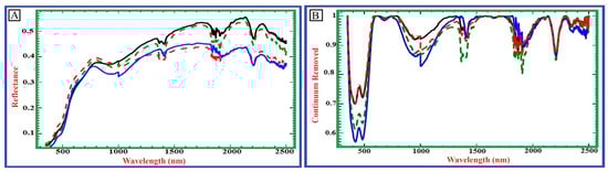
Figure 3. Examples of VIS–NIR–SWIR reflectance spectra of representative soil samples collected from the study area, demonstrating spectral variability linked to differences in mineralogical composition (A). Continuum-removed spectra highlight diagnostic absorption features indicative of the dominant mineral constituents in the soils (B). Key absorption features include Fe-oxide-related bands in the visible spectrum (~450–550 nm), OH-related overtones of clay minerals (~1400 nm), H₂O-related absorptions (~1900 nm), Al–OH clay mineral features (~2200–2250 nm), and carbonate and/or Mg–OH-related absorptions (~2300–2350 nm). Each coloured curve in both panels represents the same representative soil sample, with solid and dashed lines used solely to distinguish individual samples.

Figure 4 presents a PCA score plot highlighting several anomalous spectra from collected samples that fall outside the 95% confidence ellipse, likely caused by illumination artefacts, particle-size irregularities, or surface roughness. These outliers were removed to avoid bias in subsequent modelling steps and to ensure the dataset’s statistical consistency.

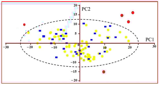
Figure 4. PCA of the absorption spectra for the studied soil samples, showing a two-dimensional plot of the first two principal components. Red circles indicate outliers, yellow circles represent calibration samples (training set), and blue squares denote validation samples. The dashed ellipse marks the 95% confidence region of the main data distribution in the PCA space. This analysis was conducted to reduce data dimensionality and enhance spectral feature extraction.

Following outlier removal, VIS–NIR–SWIR spectra were resampled at 10-nm intervals, resulting in a harmonised dataset of 205 spectral variables per sample. This resampling step improved numerical stability across applied algorithms by standardising dimensionality. Derivative processing further emphasised diagnostic mineralogical features that had previously been obscured by broad continuum curvature. Iron-oxide overtones near approximately 0.55 μm and the Al–OH/Mg–OH absorption complexes around 2.17–2.25 μm became more visible, enabling more accurate identification of mineralogical controls on trace-metal behaviour (Figure 5 and Figure 6). The quantitative benefits of the pre-processing sequence in spectral modelling are summarised in Table S3 of the Supplementary Material.

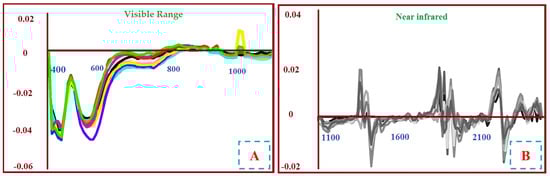
Figure 5. Raw absorption spectra of representative soil samples in the visible spectral range (~400–700 nm) (A) and in the near-infrared to shortwave infrared range (~1100–2500 nm) (B), expressed in absorbance units (A = log₁₀(1/R), where R is reflectance). Different coloured curves represent individual soil samples and illustrate inter-sample spectral variability. The absorbance representation is used here to enhance subtle and overlapping mineral absorption features and to facilitate comparison of spectral behaviour across samples. (A) highlights variability in Fe-oxide-related absorption features in the visible range, while (B) emphasises absorption characteristics linked to clay minerals, hydroxyl-bearing phases, and carbonates in the NIR–SWIR domain. In both (A) and (B), wavelength (nm) is shown on the x-axis and absorbance on the y-axis.

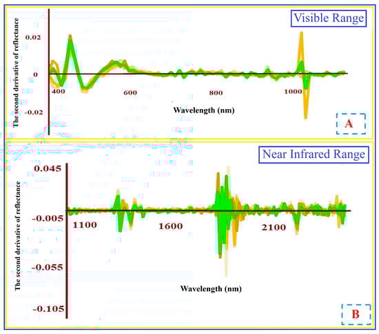
Figure 6. Second-derivative absorption spectra of representative soil samples in the visible spectral range (~400–700 nm) (A), and in the near-infrared (~1100–2500 nm) (B). The spectra emphasise key absorption features related to mineralogical and geochemical properties of the soils. In both (A) and (B), the x-axis indicates wavelength (nm). Each coloured curve in the two graphs corresponds to the same representative soil sample.

4.3. Spectral Feature Selection

Pre-processed VIS–NIR–SWIR spectra revealed distinct, element-specific wavelength relationships that align with known mineralogical controls on trace-metal retention and mobility in hydrothermally altered soils. These relationships only became apparent after derivative transformation, which enhanced subtle, overlapping absorption features and enabled the identification of diagnostically relevant spectral domains associated with Fe-oxides, phyllosilicates, and carbonate-rich matrices. Since trace metals do not show direct electronic absorptions in the VIS–NIR–SWIR range, their spectral predictability is inherently indirect and is controlled by mineral phases that influence metal sorption, substitution, and surface complexation.

Chromium showed notable spectral responses in the visible region around 540–560 nm, near 1400 nm, and in the SWIR region around 2200 nm. The visible wavelengths correspond to Fe-oxide-related ligand-field transitions, indicating Cr’s strong affinity for Fe-bearing phases via substitution and adsorption mechanisms. The significance of the ~1400 nm region does not denote direct Cr absorption but instead reflects OH-related absorptions in clay minerals, such as kaolinite and smectite, which serve as indirect mineralogical proxies that influence Cr retention. Similarly, the ~2200 nm region corresponds to Al–OH and Mg–OH vibrational features typical of phyllosilicates that affect Cr distribution through cation exchange and surface complexation.

Arsenic showed diagnostic spectral responses primarily in the visible spectrum, between approximately 460 and 580 nm. These wavelengths are associated with Fe-oxide absorption features and are consistent with the well-documented regulation of As mobility and accumulation by adsorption and co-precipitation on Fe-oxides. Additional contributions in the SWIR region further indicate the influence of clay minerals on As retention, reinforcing the indirect mineralogical basis of the observed spectral–geochemical relationships.

Copper exhibited correlated spectral features at 470, 660, 1280, and 2210 nm, indicating its association with hematite-rich, clay-dominated soil fractions. The features in the visible region relate to Fe-oxides and organic–mineral complexes that influence Cu adsorption, while the SWIR responses suggest the involvement of clay minerals and carbonate phases that provide additional sorption sites under different geochemical conditions.

Cadmium, which has no direct absorptions in the VIS–NIR–SWIR domain, displayed consistent spectral shoulders near 570 nm, around 920 nm, close to 1390 nm, and throughout the 2200–2340 nm range. These wavelength regions are associated with Fe-oxides, phyllosilicates, and carbonate-related absorption bands, which serve as indirect mineralogical indicators of Cd binding and retention via cation exchange and surface complexation.

The contribution of the ~1400 nm region indicates OH-related mineral absorptions rather than moisture effects. All soil samples were oven-dried prior to spectral measurement and analysed under controlled laboratory conditions, minimising the influence of soil moisture and atmospheric water absorption near 1400 and 1900 nm. Moreover, spectral trimming, scatter correction, and derivative pre-processing significantly reduced the impact of residual water-related absorptions while highlighting mineral-specific spectral features relevant for trace-metal estimation.

Additional support for these wavelength–metal relationships is provided by the GA feature selection results (Figure 7), which identify spectral intervals exhibiting the strongest covariance with laboratory-measured metal concentrations. The GA-selected bands cluster within mineralogically interpretable absorption regions, reinforcing the idea that trace-metal predictability in the VIS–NIR–SWIR spectrum arises from indirect mineralogical proxies rather than metal-specific absorptions. Derivative-based correlation analysis further clarifies these relationships (Figure 8), with each element (Cr, As, Cu, and Cd) displaying distinct correlation peaks that coincide with Fe-oxide, Al–OH, and Mg–OH absorption features.

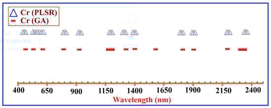
Figure 7. Wavelength intervals identified by the GA and PLSR as the most informative spectral features for predicting soil Cr concentrations from VIS–NIR–SWIR spectra using indirect mineralogical proxies. The selected intervals largely match mineralogically diagnostic absorption characteristics, including Fe-oxide-related electronic transitions in the visible range (~540–560 nm) and OH-related clay mineral absorptions in the NIR–SWIR regions around ~1400 nm and ~2200–2250 nm. The distribution of chosen wavelengths indicates that Cr predictability mainly depends on indirect mineralogical proxies rather than direct spectral responses of chromium.

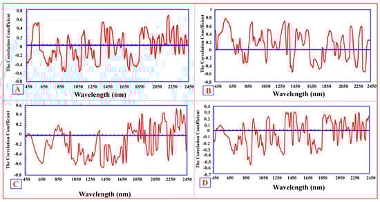
Figure 8. First-derivative spectral correlation profiles between VIS–NIR–SWIR reflectance and laboratory-measured concentrations of Cr (A), As (B), Cu (C), and Cd (D). Correlation maxima generally occur near mineralogically interpretable absorption features, including Fe-oxide-related ligand-field transitions in the visible region (~460–580 nm) and OH-bearing clay and carbonate absorptions in the NIR–SWIR regions (~1400, ~2200, and ~2300 nm). These element-specific correlation patterns suggest that trace-metal predictability mainly relates to indirect mineralogical controls rather than to direct electronic absorption by the metals themselves.

The importance of the identified wavelength regions is independently supported by PLSR loading patterns (Figure 9). Dominant loadings consistently highlight the same spectral areas previously selected by the GA and confirmed through derivative-based correlation analysis, indicating that these features reflect genuine mineralogical differences rather than artefacts of model optimisation. The observed loading peaks align with mineralogically interpretable absorption features within the VIS–NIR–SWIR spectral range, underscoring their physical significance for trace-metal prediction.

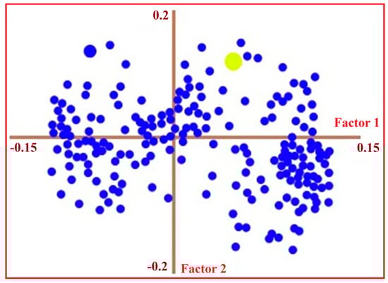
Figure 9. PLSR loading plot showing the contribution of individual spectral variables across the VIS–NIR–SWIR domain to the variance structure of the chosen trace-metal prediction model. Each point indicates a wavelength variable projected onto the first two latent factors (Factor 1 and Factor 2), which account for the greatest proportion of covariance between spectral data and measured trace-metal concentrations. The highlighted light-green point marks the wavelength with the highest absolute loading value, indicating the spectral region with the strongest influence on modelling performance.

Together, these results establish a consistent spectral–geochemical framework in which diagnostic mineralogical proxies—primarily Fe-oxides, clay minerals, and carbonate phases—govern trace-metal estimates. The agreement among GA-selected wavelengths, derivative-based correlations, and PLSR loading structures confirms the robustness and reproducibility of these spectral–metal relationships. This integrated validation provides a solid foundation for future predictive modelling across the study area.

4.4. Modelling Prediction, Evaluation and Mapping

Using the GA-selected and derivative-enhanced spectral features as input variables, spectral predictive modelling with ANNs, SVR, PLSR, and SMLR was performed. As noted earlier, the performance of all models was assessed using R²_p, RMSEP, and RPD metrics. The overall results for the four selected soil trace metals are summarised in Table 2, where the nonlinear approaches (ANNs and SVR) consistently outperform the linear techniques (PLSR and SMLR).

Table 2. Results of the overall performance of the spectral predictive modelling conducted for the selected geochemical elements (Cr, As, Cu, and Cd).

Modelling Approach	R2p	RMSEP	RPD
ANNs	0.83	1.06	2.61
SVR	0.78	1.15	2.24
PLSR	0.72	1.82	2.1
SMLR	0.65	2.05	1.92

When analysing each element individually, the behaviour of the spectral modelling approaches varies considerably (see Tables S4–S7 of the Supplementary Materials). For Cr, a clear trend emerges: predictive accuracy steadily improves as the complexity of the derivative or pre-processing increases, and among all configurations, the second-derivative ANNs achieve the highest performance. For As, the first-derivative SVR performed best, as evidenced by spectral group error patterns. Figure 10 displays the PLSR-derived diagnostic wavelengths related to As prediction, while Figure 11 illustrates the corresponding loading profiles highlighting As-sensitive spectral intervals. In addition to scalar prediction accuracy, a comparative plot of predicted versus measured As-concentrations for PLSR and SVR is shown in Figure 12, confirming SVR’s superior alignment in the validation space.

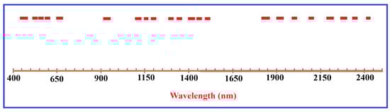
Figure 10. Wavelengths chosen by the PLSR model as the most informative spectral variables for trace-element prediction in the studied soil samples across the VIS–NIR–SWIR range (~400–2500 nm). Red markers denote wavelengths with high significance in the PLSR model, indicating spectral regions linked to mineralogical absorption features that indirectly affect trace-element variability. These selected wavelengths emphasise the spectral domains that contribute most significantly to the modelling performance.

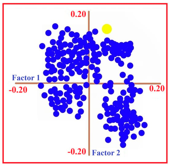
Figure 11. PLSR loading plot showing the distribution of spectral variables linked to As concentration in soil samples from the study area. Blue points indicate individual spectral loadings across the VIS–NIR–SWIR domain, while the highlighted yellow point emphasises a wavelength with a relatively high loading magnitude, suggesting its greater contribution to the PLSR model.

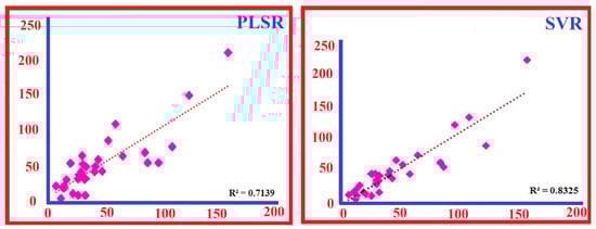
Figure 12. Comparative performance of PLSR and SVR models in predicting As concentrations in soil samples from the study area. Scatter plots display predicted versus measured As concentrations for the PLSR (left) and SVR (right) models, with modelling performance assessed using the coefficient of determination (R²). In both panels, measured As concentrations are shown on the x-axis and predicted As concentrations on the y-axis. The SVR model demonstrates higher predictive accuracy (R² = 0.8325) compared to the PLSR model (R² = 0.7139).

For Cu, the modelling results showed significant improvements with derivative-based pre-processing, with the first-derivative SMLR achieving the highest predictive accuracy (R²_p = 0.92, RPD = 3.43, RMSEP = 0.96). Among nonlinear ML-based techniques, ANNs performed well under derivative transformations (R²_p = 0.82 for the first derivative), while SVR showed moderate but consistent results across all pre-processing options. In contrast, the PLSR demonstrated comparatively lower accuracy, confirming that derivative-enhanced linear and nonlinear techniques are more effective at capturing the spectral–geochemical relationships that influence Cu variability in the study area. Cd benefits greatly from derivative enhancement combined with a linear regression strategy, achieving the best performance with the first-derivative SMLR.

Spatial prediction diagnostics derived from model residuals were employed to assess the suitability of the regression outputs for kriging. For Cr and As, the variogram parameters, including nugget, sill, and effective range, are summarised in Table 3, confirming the presence of moderate spatial continuity within each element’s residual structure. The corresponding variogram characteristics for Cu and Cd are shown in Table 4, demonstrating similar behaviour and supporting subsequent spatial interpolation.

Table 3. Variogram parameters for Cr and As, including nugget, sill, sill/nugget ratio, effective range, and kriging cross-validation RMSE.

Element	Nugget	Sill	Sill/Nugget	Effective Range	RMSE
Cr	0.745	0.868	0.85	442	1.07
As	0.475	0.862	0.552	561	0.95

Table 4. Variogram parameters for Cu and Cd, including nugget, sill, sill/nugget ratio, effective range, and kriging cross-validation RMSE.

Element	Nugget	Sill	Sill/Nugget	Effective Range	RMSE
Cu	0.313	0.924	0.338	456	0.82
Cd	0.372	0.831	0.48	372	0.88

Collectively, these results indicate that nonlinear models (ANNs and SVR) deliver the strongest overall predictive performance for most selected elements. Meanwhile, derivative-enhanced linear approaches, such as first-derivative SMLR and PLSR, can outperform nonlinear methods for Cu and Cd concentrations. The convergence of scalar performance metrics, wavelength-selection behaviour, and variogram diagnostics confirms the internal consistency of the modelling framework and its appropriateness for integration with external validation and spatial prediction mapping.

Additionally, the results of external validation for ANNs and SVR, using the 25 soil samples that were entirely excluded from previous calibration and internal cross-validation, are reported in Table 5, where ANNs consistently achieved the highest external predictive accuracy across the considered trace metal concentrations.

Table 5. External validation results for the ML-based approaches (ANNs and SVR) for predicting As, Cr, and Cu concentrations using an independent test dataset.

Element	Approach	R2p	RMSEP	RPD
As	ANNs	0.929	3.35	3.76
As	SVR	0.877	4.41	2.85
Cr	ANNs	0.82	5.74	2.35
Cr	SVR	0.39	10.56	1.28
Cu	ANNs	0.867	4.45	2.74
Cu	SVR	0.707	6.61	1.85

To visualise the alignment between predicted and observed concentrations, Figure 13 shows scatter plots for Cr, As, and Cu using both ANNs and SVR. Error diagnostics confirmed the reliability of these predictions. The residual–prediction plots in Figure 14 demonstrate that errors for both ANNs and SVR are symmetrically distributed around zero, with no visual signs of heteroscedasticity. This pattern indicates consistent modelling performance throughout the entire concentration range. Further examination of prediction uncertainties was performed using histogram analysis. As shown in Figure 15, the prediction error distributions for Cr, As, and Cu resemble a normal distribution across both ML-based modelling approaches. The slight skewness observed in the distributions of As-ANNs and Cu-ANNs appears minor and does not influence the overall predictive behaviour.

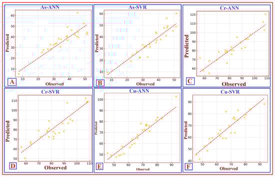
Figure 13. Scatter plots showing the predicted versus observed concentration values for soil trace elements using different ML-based approaches. These include the predicted As by the ANN (As–ANN) (A); the As predicted by the SVR (As–SVR) (B); the Cr predicted by the ANN (Cr–ANN) (C); the Cr predicted by the SVR (Cr–SVR) (D); the Cu predicted by the ANN (Cu–ANN) (E); and the Cu predicted by the SVR (Cu–SVR) (F). The red dashed line indicates the 1:1 line, representing good agreement between predicted and observed values and demonstrating the model’s predictive accuracy.

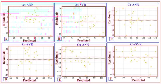
Figure 14. Scatter plots showing the residuals versus predicted concentration values for soil trace elements using different ML-based approaches. These include the residuals of As predicted by the ANN (As–ANN) (A); the residuals of As predicted by the SVR (As–SVR) (B); the residuals of Cr predicted by the ANN (Cr–ANN) (C); the residuals of Cr predicted by the SVR (Cr–SVR) (D); the residuals of Cu predicted by the ANN (Cu–ANN) (E); and the residuals of Cu predicted by the SVR (Cu–SVR) (F). The red dashed line indicates zero residuals, and the distribution of residuals around this line confirms the absence of bias. The randomness and symmetry of the residuals suggest that both modelling procedures are stable and unbiased, with no signs of heteroscedasticity or systematic errors across the prediction range.

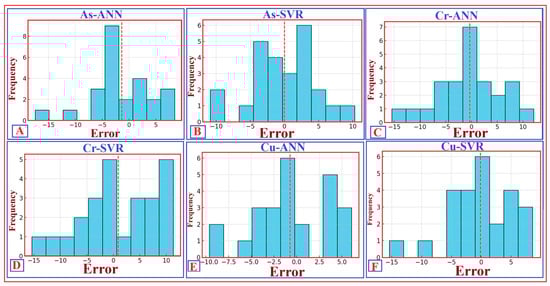
Figure 15. Histograms depict the distributions of prediction errors for soil trace element concentrations using different ML-based approaches. These include the error distribution for As predicted by the ANN (As–ANN) (A); the error distribution for As predicted by the SVR (As–SVR) (B); the error distribution for Cr predicted by the ANN (Cr–ANN) (C); the error distribution for Cr predicted by the SVR (Cr–SVR) (D); the error distribution for Cu predicted by the ANN (Cu–ANN) (E); and the error distribution for Cu predicted by the SVR (Cu–SVR) (F). The red-dashed line indicates the zero-error line, which shows the central tendency of the errors. The histograms mainly show symmetric error distributions, with some mild skewness in As-ANN and Cu-ANN, likely due to local variations in spectral behaviour or geochemical anomalies. The distributions suggest that both modelling approaches offer reliable predictions with only minor deviations from the actual values.

Finally, to assess local deviations and the smoothness of error distributions, kernel density functions were calculated. The resulting curves, shown in Figure 16, are unimodal and centred near zero for all models and elements, confirming that deviations between predicted and observed concentrations are minimal and largely symmetric.

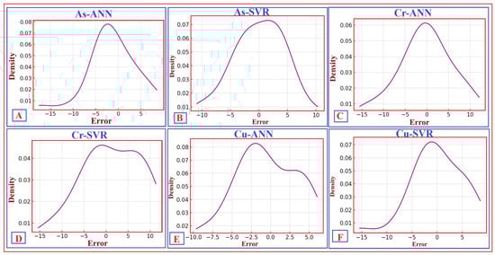
Figure 16. Kernel density plots showing the distribution of prediction errors for soil trace element concentrations using different ML-based approaches. These include the error density for As predicted by the ANN (As–ANN) (A); the error density for As predicted by the SVR (As–SVR) (B); the error density for Cr predicted by the ANN (Cr–ANN) (C); the error density for Cr predicted by the SVR (Cr–SVR) (D); the error density for Cu predicted by the ANN (Cu–ANN) (E); and the error density for Cu predicted by the SVR (Cu–SVR) (F). The plots display nearly unimodal, symmetric distributions centred around zero, indicating that most errors are minor and that the models provide accurate predictions. Slight deviations from perfect symmetry are observed for As-ANN and Cu-ANN, suggesting minor local variations or anomalies in spectral behaviour.

Overall, the external validation results demonstrate that both ANNs and SVR generalise effectively to new samples, with ANNs consistently delivering higher predictive accuracy. The close agreement between observed and predicted external concentrations, along with stable and well-behaved error distributions, affirms the robustness of the proposed nonlinear methods for spectral modelling and supports their use in subsequent spatial interpolation of selected geochemical elements and mapping.

To convert point-based predictions into continuous concentration fields, ordinary kriging was applied using variograms derived from modelling residuals. Effective ranges of approximately 442 m for Cr, 561 m for As, 456 m for Cu, and 372 m for Cd (Table 3 and Table 4), combined with low cross-validation errors, suggest moderate yet meaningful spatial autocorrelation. The resulting maps accurately reflect the measured geochemical heterogeneity (Figure 17).

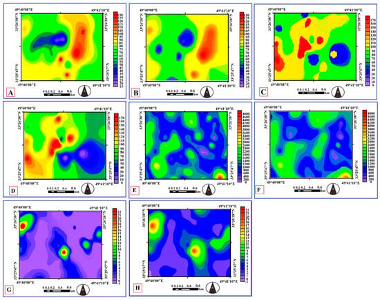
Figure 17. Spatial distribution maps of measured (A,C,E,G) and model-predicted (B,D,F,H) soil concentrations of Cr, As, Cu, and Cd in the study area. Measured grid surfaces were generated using ordinary kriging applied to geochemical assays, and predicted surfaces were interpolated from spectral modelling outputs. Values are expressed in mg/kg. These spatial patterns should be interpreted alongside Figure 1, which provides the geological context for the observed trace-metal distributions.

5. Discussion

5.1. Modelling Performance and Predictive Fidelity

Benchmarking the four spectral modelling approaches reveals a clear hierarchy in their ability to capture nonlinear spectral–geochemical relationships. Across all selected trace metals, nonlinear algorithms (ANNs, SVR) consistently outperform linear baselines (PLSR, SMLR), confirming the well-documented suitability of neural- and kernel-based models for high-dimensional, collinear soil spectra [110,111]. The ANNs approach achieves the highest overall predictive accuracy (R²_p = 0.83; RMSEP = 1.06), with element-specific gains notably pronounced for Cr (R²_p = 0.92).

Derivative-based pre-processing proved vital for enhancing subtle absorption features and reducing scattering noise, aligning with established theory [58]. First- and second-order derivatives enhanced the detectability of diagnostic clay, Fe-oxide, and carbonate features, explaining the superior results of derivative-enhanced approaches, most notably the second-derivative ANNs for Cr, the first-derivative SVR for As, the first-derivative SMLR for Cu, and the first-derivative PLSR for Cd. These improvements show that derivative transformations pinpoint chemically meaningful inflexion points that relate to mineralogical proxies of metal retention.

Variations in ANNs performance among individual elements mainly stem from differences in the strength and complexity of their spectral–mineralogical coupling. Elements like Cr and As are closely associated with spectrally active mineral phases, especially Fe-oxides and clay minerals, which display diagnostic but overlapping absorption features in the VIS–NIR–SWIR range. These interactions result in nonlinear spectral responses that are effectively modelled by ANN architectures. Conversely, elements such as Cu and Cd are often present at trace levels, in sulfide phases, or in organic–metal complexes, producing weaker or more indirect spectral signals, thereby limiting the effectiveness of highly nonlinear models.

The integration of GA-based feature selection further enhanced predictive accuracy by decreasing spectral redundancy and pinpointing the most informative wavelengths. The resulting ANNs and SVR models demonstrated minimal bias, random residuals, and near-normal error structures. External validation confirmed strong generalisability (e.g., ANN R² values of 0.929 for As, 0.867 for Cu, 0.82 for Cr), showing that high-resolution VIS–NIR–SWIR spectroscopy, when combined with derivative filtering and targeted feature reduction, can produce reliable geochemical estimates even without MIR inputs.

Together, these findings demonstrate that computational optimisation can address spectral gaps and highlight the benefits of physically informed spectral pre-processing in ML-based geochemical modelling.

5.2. Geological Controls and Mineral–Metal Coupling

The integrated geochemical, spectral, and spatial analyses demonstrate that the distributions of Cr, As, Cu, and Cd in the study area are primarily governed by lithological heterogeneity, alteration mineralogy, and the tectono-magmatic fabric of the SSZ. The strong association between diagnostic VIS–NIR–SWIR absorption features and metal-enriched zones suggests that the models developed capture mechanistic mineralogical interactions rather than merely empirical correlations, in accordance with previous soil spectroscopy studies [110]. This convergence underscores the reliability of the employed techniques in hydrothermally altered terrains where soil formation closely relates to underlying lithology and weathering processes.

Cr shows characteristic spectral responses near 540–550 nm, 1400 nm, and around 2200 nm, corresponding to overtone and combination bands of kaolinite and montmorillonite minerals that are known to retain Cr through cation exchange and surface complexation mechanisms [7,112]. The spatial clustering of Cr anomalies along ultramafic units and fault-controlled alteration belts highlights the combined influence of hydrothermal remobilisation and subsequent weathering, aligning with regional tectono-magmatic reconstructions [49,54]. Additionally, Cr demonstrates strong spectral coupling with ferric iron oxides, evidenced by absorption features between 460 and 580 nm characteristic of hematite and goethite [113]. The spatial coincidence of Cr enrichment with Fe-oxide-rich horizons supports redox-controlled adsorption as a dominant immobilisation process [114].

Cu and Cd show similar mineralogical associations. Cu spectral features at roughly 470, 660, and 2210 nm are consistent with sorption onto hematite and aluminosilicate phases [115], while Cd exhibits broader responses between 1390 and 2340 nm, indicating its preferential association with phyllosilicates and secondary carbonate minerals [35]. These element-specific yet convergent spectral signatures highlight the importance of alteration-driven mineralogical variability as the main factor influencing trace-metal retention across the study area.

The robustness of these spectral–geochemical relationships, however, is affected by geomorphological and pedogenetic context. In regions dominated by residual soils formed in place, the VIS–NIR–SWIR response accurately indicates local mineralogical assemblages, creating a strong link between spectral features and trace-metal concentrations. Conversely, areas influenced by colluvial or alluvial regolith transport may show partial decoupling from local bedrock geology due to sediment mixing, varying provenance, and post-depositional reworking. In such conditions, trace-metal distributions are influenced by upstream lithologies and secondary weathering processes, thereby increasing spatial uncertainty. Nonetheless, because the proposed framework relies on mineralogical proxies—particularly Fe-oxides, clay minerals, and carbonate phases—rather than direct metal absorptions, it remains valid in transported settings as long as these sorptive phases dominate the soil matrix.

Ordinary kriging was used to convert point-based measurements and model predictions into continuous geochemical surfaces. Spherical variogram models show moderate spatial autocorrelation, with effective ranges of 442–561 m for Cr and As, and 372–456 m for Cd and Cu. Nugget-to-sill ratios below 0.5 indicate significant spatial structure, supporting the suitability of kriging for interpolation. The resulting prediction maps display strong spatial coherence, with metal enrichment zones aligning with recognised SSZ tectono-stratigraphic boundaries and hydrothermal alteration belts [116].

As noted by [117], ordinary kriging can introduce smoothing effects and yield relatively coarse spatial resolution, potentially reducing the accuracy of heavy metal mapping in geologically complex areas. In our study, several factors help to mitigate these limitations. The soil sampling network was designed to capture the main lithological and tectono-stratigraphic variability, reducing undersampling effects that often amplify smoothing. Spherical variogram models were carefully fitted for each metal to accurately represent both short- and medium-range spatial autocorrelation, thereby preserving meaningful local heterogeneity. Cross-validation confirmed that kriging predictions were unbiased and accurate, while integrating measured data with derivative spectral and ML-based predictions further improved effective spatial resolution and accounted for local variations that kriging alone might smooth out.

Localised mismatches between observed and predicted values, most evident for Cd, likely reflect residual micro-scale heterogeneity or local variations in soil chemistry. These discrepancies could be further addressed in future work by incorporating additional environmental covariates (e.g., pH, organic carbon, and moisture content) or by applying advanced geostatistical approaches such as co-kriging and sequential Gaussian simulation [118,119]. By combining careful sampling, variogram modelling, cross-validation, and integration with predictive models, our approach provides a statistically robust representation of soil heavy metal distributions while maintaining meaningful spatial detail, despite the inherent limitations of ordinary kriging.

5.3. Environmental and Practical Implications

The mapped geochemical heterogeneity offers essential insights for environmental management in the Zagros region. Elevated Cr and Cu levels coincide with ultramafic and hematitic terrains, indicating mainly geogenic enrichment [47,55]. In contrast, the more localised As and Cd hotspots linked to drainage networks and alteration zones suggest secondary mobilisation driven by redox fluctuations and hydro-climatic processes [50].

Predicted concentrations of As (≈35 mg kg⁻¹) and Cd (≈2.5 mg kg⁻¹) surpass WHO/FAO [120] thresholds in several sub-catchments, indicating potential ecological and human health risks under varying moisture and redox conditions. The potential ecological risk index (PERI) yields an RI ≈ 156, categorising the study area as having a low-to-moderate ecological risk, predominantly due to Cd (Erᵢ ≈ 62) and As (Erᵢ ≈ 48). Consequently, these elements warrant targeted monitoring.

The demonstrated predictive accuracy and spatial fidelity of VIS–NIR–SWIR with ML–kriging integration highlight its usefulness as a quick, non-destructive, scalable alternative to laboratory-based ICP–MS and XRF analyses [8,9]. The workflow developed here, including derivative pre-processing, GA-based wavelength selection, multi-model benchmarking, and geostatistical interpolation, can be applied to other geologically complex regions. Paired with field-deployable VIS–NIR sensors, this approach can support real-time hotspot detection, land-use planning, agricultural management, and contamination mitigation in orogenic terrains.

5.4. Limitations and Future Perspectives

Although the modelling framework demonstrated strong predictive capacity and spatial accuracy, several limitations should be acknowledged to guide future methodological enhancements and remote sensing applications. First, the sample size (110 + 25) restricts the ability to fully address micro-scale heterogeneity, especially in geologically complex areas where weathering gradients, alteration fronts, and soil mineralogical transitions occur over short distances. Increasing sampling density, particularly across fault-controlled alteration belts and along drainage networks, would reduce kriging uncertainty and improve model stability. Although the calibration dataset is moderate relative to the dimensionality of hyperspectral data, effective modelling complexity was substantially constrained through derivative-based pre-processing and GA-driven wavelength selection, and robust generalisation was confirmed using nested, spatial/block, and external validation, thereby reducing the risk of overfitting in high-dimensional spectral space.

Second, while VIS–NIR–SWIR spectroscopy captured key mineralogical proxies for Cr, As, Cu, and Cd, specific soil processes, such as organic–metal complexation, micro-aggregate effects, and poorly crystalline Fe phases, produce weak or ambiguous spectral signals. Extending the spectral range to include MIR (e.g., 2500–25,000 nm), where fundamental vibrations of clays, carbonates, and organic compounds are more prominent, may further enhance predictive accuracy, in line with prior studies emphasising MIR’s benefits in soil chemistry estimation [121].

It should be emphasised that this study does not perform direct or synchronous inversion of airborne or spaceborne hyperspectral imagery in mountainous terrain. Instead, laboratory VIS–NIR–SWIR spectroscopy was deliberately used to establish physically interpretable spectral–geochemical relationships under controlled conditions, thereby eliminating topographic, illumination, and adjacency effects that commonly degrade airborne and satellite observations in rugged landscapes. The derivative-based pre-processing and mineralogical proxy approach adopted here relies on absorption feature positions and shapes rather than absolute reflectance magnitudes, making the framework inherently robust to illumination-induced spectral distortions. Future extension of this workflow to airborne or satellite hyperspectral data will nevertheless require explicit topographic and bidirectional reflectance distribution function corrections [122] to preserve predictive accuracy at the regional scale.

Third, uncertainty propagation remains a vital area for development in operational remote sensing. Although nested cross-validation, external validation, and bootstrap resampling confirmed high model stability, future efforts should incorporate Bayesian inference, ensemble modelling, and Monte Carlo error propagation to more accurately quantify prediction intervals [42]. Such approaches would improve transparency and facilitate risk-based decision-making for environmental monitoring authorities.

In terms of geospatial modelling, local inconsistencies, especially for Cd, probably reflect lithological anisotropy and sub-sampling of fine-scale sedimentary patches. Adding additional predictors, typically available from remote sensing platforms (e.g., NDVI, soil moisture indices, terrain derivatives, SWIR mineralogical indices), could reduce mapping uncertainty and improve the representativeness of spatial interpolation. The intentional exclusion of auxiliary environmental covariates in the present study allowed isolation of spectral–mineralogical controls on trace-metal behaviour and avoided location-driven overfitting; their integration is therefore viewed as a logical extension for future operational mapping rather than a prerequisite for validating the spectral–ML relationships established here. Hybrid methods, including co-kriging, regression kriging, or ML geostatistical ensembles, might further improve spatial predictions in structurally complex terrains.

From an applied remote sensing perspective, the demonstrated ability of spectral-ML integration to quantify trace metals in heterogeneous orogenic environments has important implications. The method can be expanded to imagery spectroscopy platforms such as PRISMA, EnMAP, DESIS, and upcoming missions, including CHIME (see https://www.eoportal.org/ (accessed on 10 January 2026)), enabling object-based detection of geochemically enriched zones across large areas. The mechanistic links identified between spectral characteristics and mineral–metal associations provide a strong basis for developing transferable spectral indicators of soil metal dynamics. When used with handheld sensors suitable for field deployment, these spaceborne capabilities can support rapid environmental risk assessments, near-real-time hotspot detection, and sustainable land-use planning, particularly in regions where laboratory testing is logistically or economically challenging.

Overall, while additional sampling, advanced uncertainty quantification, and the incorporation of supplementary environmental data could further improve predictive modelling, the present study develops a practical, transferable spectral–ML–geostatistical workflow that is directly applicable to remote sensing in environmental geochemistry, soil monitoring, and mineralogical mapping.

6. Conclusions and Recommendations

This study demonstrates that combining VIS–NIR–SWIR spectroscopy with derivative spectral pre-processing, GA feature selection, ML-based modelling, and geostatistical interpolation methods offers a reproducible and scalable framework for predicting and mapping soil trace metals (Cr, As, Cu, and Cd) in geologically complex orogenic terrains. The transparent benchmarking of modelling components addresses major reproducibility issues that have constrained the wider practical use of spectroscopic techniques in environmental geochemistry.

Systematic evaluation of pre-processing, feature-selection strategies, and model types confirms that derivative transformations and GA-based wavelength reduction are essential for enhancing diagnostic absorption features and stabilising modelling performance. Nonlinear algorithms—particularly ANNs and SVR—consistently outperform linear approaches, emphasising the importance of adaptable learning structures for capturing nonlinear spectral–geochemical relationships in heterogeneous soils. These findings highlight the need to carefully match modelling complexity to soil mineralogical variability and geochemical processes.

The use of nested, spatial/block, and external validation shows that the proposed workflow achieves strong generalisation under real-world conditions, reducing overfitting and increasing confidence in predictive performance. The demonstrated reliability supports applying this framework to decision-making tasks such as environmental assessment, agricultural management, and contamination risk mitigation. However, the results also indicate that modelling performance still depends on sampling density and the representativeness of training datasets, especially in highly diverse environments.

Combining spectral–ML predictions with geostatistical interpolation produces spatially continuous, geologically meaningful soil trace-metal maps. The identified mineral–metal associations—Cr with clay minerals, As with ferric iron oxides, Cu with hematite and aluminosilicates, and Cd with phyllosilicates and carbonates—correlate spatially with the main tectonostratigraphic structures of the Sanandaj–Sirjan Zone. Environmentally, the results suggest mostly geogenic enrichment of Cr and Cu in ultramafic and hematitic units, whereas As and Cd hotspots are linked to redox-sensitive drainage pathways. Several sites exceed international soil guideline standards, emphasising the importance of targeted monitoring and risk-based land-use planning.

The robustness of the proposed framework is greatest in residual soils where spectral responses directly reflect local mineralogical compositions and weathering processes. In areas affected by colluvial or alluvial transport, trace-metal patterns may combine mixed sediment sources, requiring careful interpretation while remaining manageable through mineralogical proxy-based modelling.

To improve transferability, future research should evaluate the robustness of this framework across regions with different climates, weathering regimes, soil-forming processes, and mineralogical compositions. Considering the indirect nature of spectral–metal relationships, it is advisable to develop adaptable, region-specific training datasets to accurately reflect variations in mineralogical controls and enhance both linear and nonlinear predictive models. Comparative studies across multiple regions will be especially valuable for identifying thresholds where nonlinear modelling approaches become necessary. Moreover, integrating multi-temporal imaging spectroscopy from emerging hyperspectral satellite missions (e.g., PRISMA, EnMAP, CHIME), along with advanced uncertainty quantification, transfer-learning strategies, and physically informed soil–process models, is recommended to boost scalability and operational reliability.

Overall, this study presents a reproducible, physically grounded, and operationally reliable method for predicting and mapping soil trace metals. By clearly integrating spectroscopy, ML, geostatistics, and geological interpretation, the proposed framework improves remote sensing applications for environmental intelligence across tectonically and lithologically diverse landscapes and provides a solid foundation for future regional-to-global monitoring efforts.

References

- Yuan, G.-L.; Sun, T.-H.; Han, P.; Li, J.; Lang, X.-X. Source identification and ecological risk assessment of heavy metals in topsoil using environmental geochemical mapping: Typical urban renewal area in Beijing, China. J. Geochem. Explor. 2014, 136, 40–47. [Google Scholar] [CrossRef]
- Wang, X.; Zhao, C.; Li, Z.; Huang, J. Modeling risk assessment of soil heavy metal pollution using partial least squares and fuzzy logic: A case study of a gully type coal-based solid waste dumpsite. Environ. Pollut. 2024, 352, 124147. [Google Scholar] [CrossRef] [PubMed]
- Komadja, G.C.; Westman, E.; Rana, A.; Vitalis, A. A machine learning approach to lithology classification in mining using measurement while drilling and exploration data. Min. Metall. Explor. 2025, 42, 1955–1973. [Google Scholar] [CrossRef]
- Tavallaie-Nejad, A.; Vila, M.C.; Paneiro, G.; Santos Baptista, J. A systematic review of machine learning algorithms for soil pollutant detection using satellite imagery. Remote Sens. 2025, 17, 1207. [Google Scholar] [CrossRef]
- Adriano, D.C. Trace Elements in Terrestrial Environments: Biogeochemistry, Bioavailability, and Risks of Metals, 2nd ed.; Springer: Berlin/Heidelberg, Germany, 2001. [Google Scholar]
- Smedley, P.L.; Kinniburgh, D.G. A review of the source, behaviour and distribution of arsenic in natural waters. Appl. Geochem. 2002, 17, 517–568. [Google Scholar] [CrossRef]
- Alloway, B.J. Heavy Metals in Soils: Trace Metals and Metalloids in Soils and Their Bioavailability, 3rd ed.; Springer: Berlin/Heidelberg, Germany, 2013. [Google Scholar]
- Clark, R.N. Spectroscopy of rocks and minerals, and principles of spectroscopy. Man. Remote Sens. 1999, 3, 3–58. [Google Scholar]
- Ben-Dor, E.; Chabrillat, S.; Demattê, J.A.M.; Taylor, G.R.; Hill, J.; Whiting, M.L.; Sommer, S. Using imaging spectroscopy to study soil properties. Remote Sens. Environ. 2009, 113, S38–S55. [Google Scholar] [CrossRef]
- Bartholomeus, H.M.; Schaepman, M.E.; Kooistra, L.; Stevens, A.; van Leeuwen, M. Spectral reflectance-based indices for soil organic carbon quantification. Geoderma 2011, 162, 230–238. [Google Scholar] [CrossRef]
- Wudil, Y.S.; Al-Osta, M.A.; Gondal, M.A.; Kunwar, S. Predicting soil moisture content based on laser-induced breakdown spectroscopy-informed machine learning. Arab. J. Sci. Eng. 2024, 49, 10021–11034. [Google Scholar] [CrossRef]
- Li, C.; Tan, X.; Li, X.; Huang, Y.; Xiang, C.; Wu, C.; Guo, J.; Xue, S. Simultaneous stabilization of cadmium and arsenic in soil by humic acid and mechanically activated phosphate rock. J. Hazard. Mater. 2025, 489, 137628. [Google Scholar] [CrossRef] [PubMed]
- Chabrillat, S.; Ben-Dor, E.; Cierniewski, J.; Gomez, C.; Schmid, T.; van Wesemael, B. Imaging spectroscopy for soil mapping and monitoring. Surv. Geophys. 2019, 40, 361–399. [Google Scholar] [CrossRef]
- Lagacherie, P.; Baret, F.; Feret, J.-B.; Madeira Netto, J.; Robbez-Masson, J.-M. Estimation of soil clay and calcium carbonate using laboratory, field and airborne hyperspectral measurements. Remote Sens. Environ. 2008, 112, 825–835. [Google Scholar] [CrossRef]
- Lobell, D.B.; Asner, G.P. Moisture effects on soil reflectance. Soil Sci. Soc. Am. J. 2002, 66, 722–727. [Google Scholar] [CrossRef]
- Zhai, Y.; Zhou, L.; Qi, H.; Gao, P.; Zhang, C. Application of visible/near-infrared spectroscopy and hyperspectral imaging with machine learning for high-throughput plant heavy metal stress phenotyping: A review. Plant Phenomics 2023, 2023, 0124. [Google Scholar] [CrossRef]
- Kraal, K.; Ayling, B.; DeOreo, S.; Calvin, W. Infrared spectroscopy as a tool for hydrothermal alteration mineral analysis to support geothermal reservoir characterization at The Geysers, California, USA. J. Volcanol. Geotherm. Res. 2024, 445, 107968. [Google Scholar] [CrossRef]
- Li, Y.; Chen, Z.; Chen, Y.; Li, T.; Wang, C.; Li, C. Predicting the spatial distribution of soil organic carbon in the Black Soil Area of Northeast Plain, China. Sustainability 2025, 17, 396. [Google Scholar] [CrossRef]
- Sangoi, D.V.d.S.; Dalmolin, R.S.D.; Moura-Bueno, J.M.; Pedron, F.d.A.; Brunetto, G.; Hindersmann, J.; Grando, D.L.; Fontana, A.E. Combining Vis–NIR–SWIR spectroscopy and machine learning to predict soil available copper and zinc in southern Brazil vineyards. J. Soil Sci. Plant Nutr. 2025, 25, 4439–4453. [Google Scholar] [CrossRef]
- Berlanga, G.; Acosta-Maeda, T.; Sharma, S.; Porter, J.; Dera, P.; Shelton, H. Remote Raman spectroscopy of natural rocks. Appl. Opt. 2019, 58, 8971–8980. [Google Scholar] [CrossRef] [PubMed]
- Angelopoulou, T.; Balafoutis, A.; Zalidis, G.; Bochtis, D. From Laboratory to Proximal Sensing Spectroscopy for Soil Organic Carbon Estimation: A Review. Sustainability 2020, 12, 443. [Google Scholar] [CrossRef]
- Imgram, P.; Konig, K.; Kramer, J.; Ratajczyk, T.; Maab, B.; Muller, P. High-precision collinear laser spectroscopy at the Collinear Apparatus for Laser Spectroscopy and Applied Physics (COALA). Hyperfine Interact. 2020, 241, 48. [Google Scholar] [CrossRef]
- Bonifazi, G.; Bellagamba, S.; Capobianco, G.; Gasbarone, R.; Longiro, I.; Malinconico, S.; Paglietti, F.; Serranti, S. Short-wave infrared spectroscopy for on-site discrimination of hazardous mineral fibers using machine learning techniques. Sustainability 2025, 17, 972. [Google Scholar] [CrossRef]
- Scheinost, A.C.; Schulze, D.G.; Schwertmann, U. Diffuse reflectance spectra of Al-substituted goethite: A ligand field approach. Clays Clay Miner. 2008, 46, 528–536. [Google Scholar] [CrossRef]
- Coblinski, J.A.; Inda, A.V.; Demattê, J.A.M.; Dotto, A.C.; Gholizadeh, A.; Giasson, É. Identification of minerals in subtropical soils with different textural classes by VIS–NIR–SWIR reflectance spectroscopy. CATENA 2021, 203, 105334. [Google Scholar] [CrossRef]
- Mark, H.L.; Tunnell, D. Qualitative near-infrared reflectance analysis using Mahalanobis distances. Anal. Chem. 1985, 57, 1449–1456. [Google Scholar] [CrossRef]
- Deiss, L.; Margenot, A.; Culman, S.; Demyan, M. Tuning support vector machines regression models improves prediction accuracy of soil properties in MIR spectroscopy. Geoderma 2020, 365, 114227. [Google Scholar] [CrossRef]
- Barra, I.; Haefele, S.M.; Sakrabani, R.; Kebede, F. Soil spectroscopy with the use of chemometrics, machine learning and pre-processing techniques in soil diagnosis: Recent advances—A review. TrAC Trends Anal. Chem. 2021, 135, 116166. [Google Scholar] [CrossRef]
- Atalay, F. Effect of Domaining in Mineral Resource Estimation with Machine Learning. Minerals 2025, 15, 330. [Google Scholar] [CrossRef]
- Qi, C.; Wu, M.; Li, K.; Hu, T.; Armaghani, D.J.; Chen, Q.; Yilmaz, E. Identifying mining-induced chromium contamination in soil through visible–near infrared spectroscopy and machine learning. Green Smart Min. Eng. 2024, 1, 132–139. [Google Scholar] [CrossRef]
- Sangoi, D.V.d.S.; Dalmolin, R.S.D.; Moura-Bueno, J.M.; Pedron, F.d.A.; Tiecher, T.; Brunetto, G. Performance of global and regional Vis–NIR–SWIR models in predicting soil copper and zinc in vineyards in southern Brazil. Environ. Monit. Assess. 2025, 197, 319. [Google Scholar] [CrossRef]
- Jamal, M.; Liu, Y.; Gu, T.; Hu, W.; Ren, F.; Cui, S.; Li, F. Hyperspectral remote sensing and machine learning techniques for assessing soil contamination by potentially toxic elements: A case study from the Zeïda mining area, Morocco. J. Afr. Earth Sci. 2026, 234, 105912. [Google Scholar] [CrossRef]
- Es-sahly, S.; Elbasbas, A.; Naji, K.; Lakssir, B.; Faqiri, H.; Dadi, S.; Rabie, R. NIR-spectroscopy and machine learning models to pre-concentrate copper hosted within sedimentary rocks. Min. Metall. Explor. 2024, 41, 1979–1995. [Google Scholar] [CrossRef]
- Zheng, G.; Ryu, D.; Jiao, C.; Xie, X.; Cui, X.; Shang, G. Visible and near-infrared reflectance spectroscopy analysis of a coastal soil chronosequence. Remote Sens. 2019, 11, 2336. [Google Scholar] [CrossRef]
- Li, B.; Lin, K.; Liu, X.; Ma, X.; Li, X.; Wu, Z.; Li, C.; Yu, T.; Wu, T.; Yang, Z. Mechanism of cadmium (Cd) enrichment in the soil of karst areas with high geochemical background in Southwest China. Chem. Geol. 2025, 673, 122523. [Google Scholar] [CrossRef]
- Daviran, M.; Ghezelbash, R.; Hajihosseinlou, M.; Maghsoudi, A. Uncertainty quantification in genetic algorithm-optimized artificial intelligence-based mineral prospectivity models: Automated hyperparameter tuning for support vector machines and random forest. Model. Earth Syst. Environ. 2025, 11, 10. [Google Scholar] [CrossRef]
- Tsakiridis, N.L.; Keramaris, K.D.; Theocharis, J.B.; Zalidis, G.C. Simultaneous prediction of soil properties from VNIR-SWIR spectra using a localized multi-channel 1-D convolutional neural network. Geoderma 2020, 367, 114208. [Google Scholar] [CrossRef]
- Kohler, M.; Hanelli, D.; Schaefer, S.; Barth, A.; Knobloch, A.; Hielscher, P.; Cardoso-Fernandes, J.; Lima, A.; Teodoro, A.C. Lithium Potential Mapping Using Artificial Neural Networks: A Case Study from Central Portugal. Minerals 2021, 11, 1046. [Google Scholar] [CrossRef]
- Davies, R.S.; Trott, M.; Georgi, J.; Farrar, A. Artificial intelligence and machine learning to enhance critical mineral deposit discovery. Geosystems Geoenvironment 2025, 4, 100361. [Google Scholar] [CrossRef]
- El-Omairi, M.A.; El Garouani, M.; El Garouani, A. Enhanced lithological mapping via remote sensing: Employing SVM, random trees, ANN, with MNF and PCA transformations. Egypt. J. Remote Sens. Space Sci. 2025, 28, 34–52. [Google Scholar] [CrossRef]
- Li, Z.; PuBu, Z.; Chen, X.; Chen, G.; Wei, J.; Pan, D.; Jiang, X. Identifying new copper mineralization via multispectral remote sensing (MSRS) and short-wave infrared (SWIR) spectral analysis in Dingyang, Western Gangdese Belt, Xizang. Minerals 2025, 15, 1045. [Google Scholar] [CrossRef]
- Izzaddin, A.; Langousis, A.; Totaro, V.; Yaseen, M.; Iacobellis, V. A New Diagram for Performance Evaluation of Complex Models. Stoch. Environ. Res. Risk Assess. 2024, 38, 2261–2281. [Google Scholar] [CrossRef]
- Wong, T.-T.; Yeh, P.-Y. Reliable accuracy estimates from k-fold cross validation. IEEE Trans. Knowl. Data Eng. 2020, 32, 1586–1594. [Google Scholar] [CrossRef]
- Chen, Y.; Qiao, Y.; Liu, G.; Zhao, W. Integration of spectroscopy and geostatistics for mapping heavy metal pollution in peri-urban soils. J. Hazard. Mater. 2021, 416, 125856. [Google Scholar] [CrossRef]
- Li, Y.; Yuan, X.; Gan, S.; Mu, C.; Lin, Z.; Duan, X.; Shao, Y.; Wang, Y.; Hu, L. Environmentally Sustainable Lithium Exploration: A Multi-Source Remote Sensing and Comprehensive Analysis Approach for Clay-Type Deposits in Central Yunnan, China. Sustainability 2025, 17, 3732. [Google Scholar] [CrossRef]
- Li, X.; Chen, R.; Liu, F.; You, Z.; Huang, J.; Peng, J.; Li, G. Quantitative detection of soil cadmium with graphite enhancement and spectral fusion model using laser-induced breakdown spectroscopy. Comput. Electron. Agric. 2025, 229, 109831. [Google Scholar] [CrossRef]
- Alavi, M. Tectonics of the Zagros orogenic belt of Iran: New data and interpretations. Tectonophysics 1994, 229, 211–238. [Google Scholar] [CrossRef]
- Walker, R.; Jackson, J. Active tectonics and late Cenozoic strain distribution in central and eastern Iran. Tectonics 2004, 23, 1–24. [Google Scholar] [CrossRef]
- Agard, P.; Omrani, J.; Jolivet, L.; Mouthereau, F. Convergence history across Zagros (Iran): Constraints from collisional and earlier deformation. Int. J. Earth Sci. 2005, 94, 401–419. [Google Scholar] [CrossRef]
- Boschetti, T.; Segadelli, S.; Gori, F.; Antolini, G.; Bellini, L.; Raso, A.; Selmo, E.; Barbieri, M.; Iacumin, P.; Guidetti, E.; et al. A preliminary study on the effects of rainfall-related conditions on chromium increase in ultramafic-hosted springs: A possible climate change concern? Sci. Total Environ. 2025, 958, 177826. [Google Scholar] [CrossRef]
- Li, M.; Cai, Q.; Zhang, T.; Tang, H.; Li, H. Progress of complex system process analysis based on modern spectroscopy combined with chemometrics. J. Chemom. 2025, 39, e70006. [Google Scholar] [CrossRef]
- Akbari, M.; Neamatollahi, E.; Memarian, H.; Alizadeh Noughani, M. Assessing impacts of floods disaster on soil erosion risk based on the RUSLE-GloSEM approach in western Iran. Nat. Hazards 2023, 117, 1689–1710. [Google Scholar] [CrossRef]
- Heydari, S.; Bromand, S.; Zeinali, B.; Pourghasemi, E. Precipitation Forecast of Three Stations of Lorestan Province in the Next 20 Years. J. Environ. Sci. Stud. 2024, 9, 7963–7976. [Google Scholar]
- Ghasemi, A.; Talbot, C.J. A new tectonic scenario for the Sanandaj-Sirjan Zone (Iran). J. Asian Earth Sci. 2005, 26, 683–693. [Google Scholar] [CrossRef]
- Golonka, J. Plate tectonic evolution of the southern margin of Eurasia in the Mesozoic and Cenozoic. Tectonophysics 2004, 381, 235–273. [Google Scholar] [CrossRef]
- Fazlnia, A.N.; Schenk, V.; van der Straaten, F.; Mirmohammadi, M.S. Petrology, geochemistry, and geochronology of trondhjemites from the Qori Complex, Neyriz, Iran. Lithos 2009, 112, 413–433. [Google Scholar] [CrossRef]
- Nadimi, A.; Nadimi, H. Exhumation of Old Rocks During the Zagros Collision in the Northwestern Part of Zagros Mountains, Iran. Geol. Soc. Am. Bull. 2008, 65, 674–687. [Google Scholar] [CrossRef]
- Savitzky, A.; Golay, M.J.E. Smoothing and Differentiation of Data by Simplified Least Squares Procedures. Anal. Chem. 1964, 36, 1627–1639. [Google Scholar] [CrossRef]
- Dathe, F.; Dehn, F. Alkali Activation of Common Clay Deposits: Evaluation of the Suitability by an IR Spectroscopic Method. Int. J. Concr. Struct. Mater. 2024, 18, 913–929. [Google Scholar] [CrossRef]
- Owonubi, A. Copper fractions and selected soil characteristics of a tropical toposequence. J. Agric. Environ. Res. Manag. 2024, 7, 1–9. [Google Scholar]
- Omondiagbe, O.P.; Roudier, P.; Lilburne, L.; Ma, Y.; McNeill, S. Quantifying uncertainty in the prediction of soil properties using mid-infrared spectra. Geoderma 2024, 448, 116954. [Google Scholar] [CrossRef]
- Tasan, M.; Demir, Y.; Taşan, S.; Ozturk, E. Comparative analysis of different machine learning algorithms for predicting trace metal concentrations in soils under intensive paddy cultivation. Comput. Electron. Agric. 2024, 219, 108772. [Google Scholar] [CrossRef]
- Fusaro, L.; Lanni, F.; Varone, L.; Falasca, G.; Serranti, S.; Gasbarrone, R.; Gattabria, D.; Cozzolino, V.; Piccolo, A.; Manes, F. Functional traits as indicators of maize (Zea mays L.) strategies to cope with Zn, Pb and Cr heavy metal-induced stress. Chem. Biol. Technol. Agric. 2025, 12, 82. [Google Scholar] [CrossRef]
- Li, J.; Zhang, Y.; Wang, F.; Wang, L.; Liu, J.; Hashimoto, Y.; Hosomi, M. Arsenic immobilization and removal in contaminated soil using zero-valent iron or magnetic biochar amendment followed by dry magnetic separation. Sci. Total Environ. 2021, 768, 144521. [Google Scholar] [CrossRef]
- Willmott, C.J. On the Validation of Models. Phys. Geogr. 1981, 2, 184–194. [Google Scholar] [CrossRef]
- Fouad, Y.; Soltani, I.; Cudennec, C.; Michot, D. Using near-infrared spectroscopy to estimate soil water retention curves with the van Genuchten model. Geoderma 2025, 454, 117175. [Google Scholar] [CrossRef]
- Ramsey, M.H.; Thompson, M.; Hale, M. Objective evaluation of precision requirements for geochemical analysis using robust analysis of variance. J. Geochem. Explor. 1992, 44, 23–36. [Google Scholar] [CrossRef]
- Ramifehiarivo, N.; Barthes, B.; Cambou, A.; Chapuis-Lardy, L.; Chevallier, T.; Albrecht, A. Comparison of near and mid-infrared reflectance spectroscopy for the estimation of soil organic carbon fractions in Madagascar agricultural soils. Geoderma Reg. 2023, 33, e00638. [Google Scholar] [CrossRef]
- Parish, R.M. Reflectance spectroscopy as a chert sourcing method. Archaeol. Pol. 2016, 54, 115–128. [Google Scholar]
- Beriro, D.; Vane, C. Infrared spectroscopy and chemometric modelling of organic carbon measured by Rock-Eval pyrolysis of UK shale rock. Geol. Soc. Lond. Spec. Publ. 2023, 534, 165–182. [Google Scholar] [CrossRef]
- Zhao, L.; Deng, A.; Hong, H.; Zhao, J.; Algeo, T.J.; Liu, F.; Luozhui, N.; Fang, Q. Unraveling clay-mineral genesis and climate change on Earth and Mars using machine learning-based VNIR spectral modeling. Am. Mineral. 2025, 110, 217–231. [Google Scholar] [CrossRef]
- Baldridge, A.M.; Hook, S.J.; Grove, C.I.; Rivera, G. The ASTER spectral library version 2.0. Remote Sens. Environ. 2009, 113, 711–715. [Google Scholar] [CrossRef]
- Kokaly, R.F.; Clark, R.N.; Swayze, G.A.; Livo, K.E.; Hoefen, T.M.; Pearson, N.C.; Wise, R.A.; Benzel, W.M.; Lowers, H.A.; Driscoll, R.L.; et al. USGS Spectral Library Version 7: U.S. Geological Survey Data Series 1035 (61 pp.) [Data Set]; U.S. Geological Survey: Reston, VA, USA, 2017. [Google Scholar]
- Zhou, Y.; Wang, T.; Fan, F.; Chen, S.; Guo, W.; Xing, G.; Sun, J.; Xiao, F. Advances on Exploration Indicators of Mineral VNIR-SWIR Spectroscopy and Chemistry: A Review. Minerals 2022, 12, 958. [Google Scholar] [CrossRef]
- Patel, C.M.; Patel, C.D.; Rami, J.M.; Patel, K.R. Optical spectroscopic study of natural rock’s minerals. Mater. Today Proc. 2021, 43, 497–501. [Google Scholar] [CrossRef]
- Kemper, T.; Sommer, S. Estimate of heavy metal contamination in soils after a mining accident using reflectance spectroscopy. Environ. Sci. Technol. 2002, 36, 2742–2747. [Google Scholar] [CrossRef]
- Bi, Y.; Yuan, K.; Xiao, W.; Wu, J.; Shi, C.; Xia, J.; Chu, G.; Zhang, G.; Zhou, G. A local pre-processing method for near-infrared spectra, combined with spectral segmentation and standard normal variate transformation. Anal. Chim. Acta 2016, 909, 30–40. [Google Scholar] [CrossRef]
- Helland, I.S.; Næs, T.; Isaksson, T. Related versions of the multiplicative scatter correction method for preprocessing spectroscopic data. Chemom. Intell. Lab. Syst. 1995, 29, 233–241. [Google Scholar] [CrossRef]
- Santos, U.J.; Demattê, J.A.M.; Menezes, R.S.C.; Dotto, A.C.; Guimarães, C.C.B.; Alves, B.J.R.; Primo, D.C.; Sampaio, E.V.S.B. Predicting carbon and nitrogen by visible near-infrared (Vis-NIR) and mid-infrared (MIR) spectroscopy in soils of Northeast Brazil. Geoderma Reg. 2020, 23, e00333. [Google Scholar] [CrossRef]
- Wu, J.; Huang, C. Machine learning-supported determination for site-specific natural background values of soil heavy metals. J. Hazard. Mater. 2025, 487, 137276. [Google Scholar] [CrossRef] [PubMed]
- Mahalanobis, P.C. On the Generalised Distance in Statistics. Natl. Inst. Sci. India 1936, 2, 49–55, Reprint in Sankhya A 2018, 80, 1–7. [Google Scholar] [CrossRef]
- Hastie, T.; Tibshirani, R.; Friedman, J. The Elements of Statistical Learning: Data Mining, Inference, and Prediction, 2nd ed.; Springer: New York, NY, USA, 2009. [Google Scholar]
- Tsakiridis, N.L.; Tziolas, N.V.; Theocharis, J.B.; Zalidis, G.C. A genetic algorithm-based stacking algorithm for predicting soil organic matter from vis–NIR spectral data. Eur. J. Soil Sci. 2019, 70, 578–590. [Google Scholar] [CrossRef]
- Moradpouri, F.; Dolatshahi, M.B. Optimization and machine learning methods in multivariate geochemical analysis for anomaly detection. In Optimizing Solutions for Real-Life Problems; Springer: Berlin/Heidelberg, Germany, 2025; pp. 181–236. [Google Scholar]
- Baalousha, H.M. Machine learning approaches for groundwater vulnerability assessment in arid environments: Enhancing DRASTIC with ANN and Random Forest. Groundw. Sustain. Dev. 2025, 30, 101496. [Google Scholar] [CrossRef]
- Abd-Elmaboud, M.E.; Saqr, A.M.; El-Rawy, M.; Al-Arifi, N.; Ezzeldin, R. Evaluation of groundwater potential using ANN-based mountain gazelle optimization: A framework to achieve SDGs in East El Oweinat, Egypt. J. Hydrol. Reg. Stud. 2024, 52, 101703. [Google Scholar] [CrossRef]
- Lu, Q.; Liu, S.H.; Mao, W.Z.; Yu, Y.; Long, X. A numerical simulation-based ANN method to determine the shear strength parameters of rock minerals in nanoscale. Comput. Geotech. 2024, 169, 106175. [Google Scholar] [CrossRef]
- Taşan, M. Improved prediction of groundwater quality index by hybrid machine learning models in a coastal region: A case study from Southern Turkey. Int. J. Environ. Res. 2025, 19, 147. [Google Scholar] [CrossRef]
- Achite, M.; Jehanzaib, M.; Elshaboury, N.; Khan, M.U.; Pandey, K.; Mirzania, E. Evaluating performances of SVR, HBA–SVR, and COOT–SVR techniques: Monthly evaporation modeling in Algeria. Euro-Mediterr. J. Environ. Integr. 2025, 10, 5333–5350. [Google Scholar] [CrossRef]
- Chen, X.; Xiao, T.; Ma, W.; Cai, M.; Ren, Z.; Li, H.; Bi, X.; Shi, Y.; Yue, C. Study on the Impact of Vegetation Restoration on Groundwater Resources in Tianshan Mountain and Yili Valley in Xinjiang, China. Water 2024, 16, 696. [Google Scholar] [CrossRef]
- Jeihouni, M.; Valizadeh Kamran, K.; Kusak, L. Modeling and digital mapping of shallow water table depth using satellite-based spectral and thermal data: Introducing a framework for digital shallow water table mapping. Soil Tillage Res. 2025, 245, 106317. [Google Scholar] [CrossRef]
- Miyashita, Y.; Itozawa, T.; Katsumi, H.; Sasaki, S.-I. Comments on the NIPALS algorithm. J. Chemom. 1990, 4, 97–100. [Google Scholar] [CrossRef]
- Pal, M.; Foody, G.M. Evaluation of SVM, RVM and SMLR for accurate image classification with limited ground data. IEEE J. Sel. Top. Appl. Earth Obs. Remote Sens. 2012, 5, 1344–1355. [Google Scholar] [CrossRef]
- Burnham, K.P.; Anderson, D.R. Model Selection and Multimodel Inference, 2nd ed.; Springer: Berlin/Heidelberg, Germany, 2002. [Google Scholar]
- Draper, N.R.; Smith, H. Applied Regression Analysis, 3rd ed.; Wiley: Hoboken, NJ, USA, 1998. [Google Scholar]
- Varma, S.; Simon, R. Bias in error estimation when using cross-validation for model selection. BMC Bioinform. 2006, 7, 91. [Google Scholar] [CrossRef]
- Cawley, G.C.; Talbot, N.L. On over-fitting in model selection and practice. J. Mach. Learn. Res. 2010, 11, 2079–2107. [Google Scholar]
- Wold, S.; Sjöström, M.; Eriksson, L. PLS-regression: A basic tool of chemometrics. Chemom. Intell. Lab. Syst. 2001, 58, 109–130. [Google Scholar] [CrossRef]
- Chang, C.W.; Laird, D.A.; Mausbach, M.J.; Hurburgh, C.R. Near-infrared reflectance spectroscopy–principal components regression analyses. Soil Sci. Soc. Am. J. 2001, 65, 480–490. [Google Scholar] [CrossRef]
- Roberts, D.R.; Bahn, V.; Ciuti, S.; Boyce, M.S.; Elith, J.; Guillera-Arroita, G.; Hauenstein, S.; Lahoz-Monfort, J.J.; Schröder, B.; Thuiller, W.; et al. Cross-validation strategies for data with spatial structure. Ecography 2017, 40, 913–929. [Google Scholar] [CrossRef]
- Brenning, A. Spatial cross-validation and bootstrap for the assessment of prediction rules in remote sensing. R package sperrorest documentation. In Proceedings of the 2012 IEEE International Geoscience and Remote Sensing Symposium, Munich, Germany, 22–27 July 2012. [Google Scholar]
- Shrestha, S.; Kazama, F. Assessment of surface water quality using multivariate statistical techniques. Environ. Model. Softw. 2007, 22, 464–475. [Google Scholar] [CrossRef]
- Desgraupes, B. Clustering Performance Evaluation; Université Paris Ouest: Nanterre, France, 2018. [Google Scholar]
- Seabold, S.; Perktold, J. Statsmodels: Econometric and statistical modeling with Python. In Proceedings of the 9th Python in Science Conference, Austin, TX, USA, 3–28 July 2010; Available online: https://conference.scipy.org/proceedings/scipy2010/seabold.html (accessed on 8 November 2025).
- Reimers, N.; Gurevych, I. Reporting score distributions makes a difference. arXiv 2017, arXiv:1707.09861. [Google Scholar] [CrossRef]
- Ali, D.; Hayat, M.B.; Khalid, H. Artificial intelligence and machine learning models for predicting the metallurgical performance of complex sulfide ore flotation process. Miner. Process. Extr. Metall. Trans. Inst. Min. Metall. 2025, 134, 13–32. [Google Scholar] [CrossRef]
- Li, Q.; Chen, G.; Wang, D. Mineral prospectivity mapping using semi-supervised machine learning. Math. Geosci. 2025, 57, 275–305. [Google Scholar] [CrossRef]
- Goovaerts, P. Geostatistics for Natural Resources Evaluation; Oxford University Press: Oxford, UK, 1997. [Google Scholar]
- Wang, J.; Wang, B.; Zhao, Q.; Cao, J.; Xiao, X.; Zhao, D.; Chen, Z.; Wu, D. Sources analysis and risk assessment of heavy metals in soil in a polymetallic mining area in southeastern Hubei based on Monte Carlo simulation. Ecotoxicol. Environ. Saf. 2025, 290, 117607. [Google Scholar] [CrossRef] [PubMed]
- Ngoc, L.T.; Nguyen, H.; Bui, X.-N.; Tran, T.-T. Dynamic weighting and genetic algorithm-based hybrid SVR-Ridge model for improving PM2.5 forecasting in open-pit copper mines. Int. J. Min. Reclam. Environ. 2025, 1–31. [Google Scholar] [CrossRef]
- Weindorf, D.C.; Chakraborty, S.; Li, S.; Emadi, M. Unlocking the Secrets of Soil: Applying AI and Sensor Technologies for Sustainable Land Use; Elsevier: Amsterdam, The Netherlands, 2025. [Google Scholar]
- Berberian, M.; King, G.C.P. Towards a paleogeography and tectonic evolution of Iran. Can. J. Earth Sci. 1981, 18, 210–265. [Google Scholar] [CrossRef]
- Schwertmann, U.; Cornell, R.M. Iron Oxides in the Laboratory: Preparation and Characterization, 2nd ed.; Wiley-VCH: Hoboken, NJ, USA, 2007. [Google Scholar]
- Vandeuren, A.; Pereira, B.; Van de Casteele, C.; Sonnet, P.; Delmelle, P. Processes controlling geogenic arsenic distribution in soils formed from iron-rich sedimentary rocks. J. Hazard. Mater. 2025, 483, 136610. [Google Scholar] [CrossRef]
- Zhou, Q.; Liao, B.; Lin, L.; Qiu, W.; Song, Z. Adsorption of Cu(II) and Cd(II) from aqueous solutions by ferromanganese binary oxide–biochar composites. Sci. Total Environ. 2018, 615, 115–122. [Google Scholar] [CrossRef]
- Mohajjel, M.; Fergusson, C.L.; Sahandi, M.R. Cretaceous-Tertiary convergence and continental collision, Sanandaj-Sirjan zone, Western Iran. J. Asian Earth Sci. 2003, 21, 397–412. [Google Scholar] [CrossRef]
- Xu, X.; Wang, Z.; Song, X.; Zhan, W.; Yang, S. A remote sensing-based strategy for mapping potentially toxic elements of soils: Temporal-spatial-spectral covariates combined with random forest. Environ. Res. 2024, 240, 117570. [Google Scholar] [CrossRef] [PubMed]
- Wang, L.; Liu, H.; Kang, L.; Su, H.; Shu, S.; Wang, J. Spatiotemporal continuous shallow water bathymetry from a Kriged Kalman filter. Photogramm. Eng. Remote Sens. 2025, 91, 463–471. [Google Scholar] [CrossRef]
- Lei, X.; Li, J.; Chen, Y.; Huang, H. Estimation of chromium potential risk stock in karst soils: Insights from spatial and depth variations in Southwestern China. J. Hazard. Mater. 2025, 488, 137449. [Google Scholar] [CrossRef]
- World Health Organization; Food and Agriculture Organization of the United Nations. Evaluation of Certain Food Additives and Contaminants: Sixty-Seventh Report of the Joint FAO/WHO Expert Committee on Food Additives (WHO Technical Report Series, No. 940); World Health Organization: Geneva, Switzerland, 2007; Available online: https://iris.who.int/handle/10665/43646 (accessed on 8 November 2025).
- Soriano-Disla, J.M.; Janik, L.J.; Viscarra Rossel, R.A.; Macdonald, L.M.; McLaughlin, M.J. The performance of visible, near-, and mid-infrared reflectance spectroscopy for prediction of soil physical, chemical, and biological properties. Appl. Spectrosc. Rev. 2014, 49, 139–186. [Google Scholar] [CrossRef]
- Schaepman-Strub, G.; Schaepman, M.E.; Painter, T.H.; Dangel, S.; Martonchik, J.V. Reflectance quantities in optical remote sensing—Definitions and case studies. Remote Sens. Environ. 2006, 103, 27–42. [Google Scholar] [CrossRef]
Disclaimer/Publisher’s Note: The statements, opinions and data contained in all publications are solely those of the individual author(s) and contributor(s) and not of MDPI and/or the editor(s). MDPI and/or the editor(s) disclaim responsibility for any injury to people or property resulting from any ideas, methods, instructions or products referred to in the content. |
© 2026 by the authors. Licensee MDPI, Basel, Switzerland. This article is an open access article distributed under the terms and conditions of the Creative Commons Attribution (CC BY) license.