Highlights
What are the main findings?
- The first retrieval attempt of Sea Ice Concentration (SIC) in the Arctic and Antarctic regions was successfully carried out using reflected signals from multiple Global Navigation Satellite Systems (GNSS), including GPS, BDS, and Galileo, collected by the GNOS-II instrument aboard the Fengyun-3E satellite.
- A novel Random Forest Regression (RFR)-based inversion framework was proposed, incorporating “multi-GNSS system discrimination” and “rolling window prediction” to enhance retrieval accuracy and robustness.
What are the implications of the main findings?
- The proposed multi-GNSS-based SIC retrieval methodology offers a new and efficient approach for monitoring Sea Ice Concentrations in both polar regions.
- The framework’s ability to handle complex ice–water transition zones and diverse sea ice conditions across different seasons makes it a promising method for polar climate and environmental monitoring.
Abstract
Recognizing the critical role of polar Sea Ice Concentration (SIC) in climate feedback mechanisms, this study presents the first comprehensive investigation of China’s Fengyun-3E(FY-3E) GNOS-II Global Navigation Satellite System Reflectometry (GNSS-R) for bipolar SIC retrieval. Specifically, reflected signals from multiple Global Navigation Satellite Systems (GNSS) are utilized to extract characteristic parameters from Delay Doppler Maps (DDMs). By integrating regional partitioning and dynamic thresholding for sea ice detection, a Random Forest Regression (RFR) model incorporating a rolling-window training strategy is developed to estimate SIC. The retrieved SIC products are generated at the native GNSS-R observation resolution of approximately 1 × 6 km, with each SIC estimate corresponding to an individual GNSS-R observation time. Owing to the limited daily spatial coverage of GNSS-R measurements, the retrieved SIC results are further aggregated into monthly composites for spatial distribution analysis. The model is trained and validated across both polar regions, including targeted ice–water boundary zones. Retrieved SIC estimates are compared with reference data from the OSI SAF Special Sensor Microwave Imager Sounder (SSMIS), demonstrating strong agreement. Based on an extensive dataset, the average correlation coefficient (R) reaches 0.9450 in the Arctic and 0.9602 in the Antarctic for the testing set, with corresponding Root Mean Squared Error (RMSE) of 0.1262 and 0.0818, respectively. Even in the more challenging ice–water transition zones, RMSE values remain within acceptable ranges, reaching 0.1486 in the Arctic and 0.1404 in the Antarctic. This study demonstrates the feasibility and accuracy of GNSS-R-based SIC retrieval, offering a robust and effective approach for cryospheric monitoring at high latitudes in both polar regions.
1. Introduction
As climate change accelerates, the rate of sea ice melting has increased significantly [1]. Sea ice is a critical component of the Earth’s climate system [2], playing a vital role in regulating global oceanic and atmospheric circulation patterns [3]. Furthermore, accurate knowledge of sea ice conditions is essential for the safety of Arctic shipping routes and holds strategic significance in polar military operations [4]. Sea Ice Concentration (SIC), defined as the fraction of a given ocean area covered by ice, is a key parameter for assessing the state of sea ice. Accurate monitoring and analysis of SIC provide valuable insights into its spatiotemporal dynamics and potential impacts on global climate. Fortunately, advances in satellite observation technologies [5] have enabled large-scale, high-precision monitoring of sea ice coverage. Currently, various advanced techniques for sea ice detection are widely utilized, with satellite-based microwave remote sensing recognized as one of the most effective methods. The monitoring of SIC primarily relies on satellite remote sensing technologies: passive microwave radiometers (e.g., Advanced Microwave Scanning Radiometer (AMSR) series) [6] achieve daily polar coverage through microwave radiation characteristics but suffer from low spatial resolution and reduced accuracy in summer; synthetic aperture radar (SAR) [7] provides high-resolution imaging (10–100 m) but faces challenges such as long revisit cycles and complex data interpretation; and optical remote sensing (e.g., Moderate Resolution Imaging Spectroradiometer (MODIS)) [8] captures details at a spatial resolution of approximately 1 km but is severely limited by polar nights and cloud cover.
Global Navigation Satellite System Reflectometry (GNSS-R) [9] has emerged as a powerful tool for retrieving key environmental parameters, including wind speed [10,11], soil moisture [12,13,14], snow depth [15,16], and sea ice [17], by capturing L-band reflected signals from ground, airborne [18,19,20], and spaceborne platforms, offering unique advantages: (1) global coverage with high temporal resolution enabled by multi-constellation navigation satellites; (2) penetration capability through clouds and vegetation due to L-band signals; and (3) cost-effectiveness by utilizing existing GNSS signals avoiding dedicated transmitters. The Delay Doppler Map (DDM) is a critical GNSS-R observation dataset that characterizes the scattering properties of reflective surfaces. Due to the distinct surface roughness characteristics exhibited by different sea ice and water surfaces [21], their reflected signals demonstrate notable variations in both peak power and waveform energy distribution [22]. These differential characteristics establish a robust foundation for the retrieval of SIC [23].
In recent years, the application of GNSS-R technology in sea ice research has expanded significantly [24], encompassing multiple domains such as sea ice detection, thickness estimation, and classification [25,26,27,28]. With continuous advancements in model optimization methodologies, these areas have become focal points in polar remote sensing research [29,30], particularly demonstrating substantial potential in SIC retrieval [19,31].
Currently, spaceborne GNSS-R data are derived from multiple types of satellite missions, represented by pioneering experimental satellites such as the UK’s TechDemoSat-1 (TDS-1), operational observation constellations like the U.S. Cyclone Global Navigation Satellite System (CYGNSS), and domestic operational payloads including the Global Navigation Satellite System Occultation Sounder II (GNOS-II) carried on Chinese meteorological satellites such as the Fengyun-3E (FY-3E). In the field of polar sea ice observation, due to its low-inclination orbit design, the CYGNSS satellite cannot extend its coverage to high-latitude polar regions and thus lacks systematic capability for sea ice detection. Early studies in this area predominantly relied on data acquired from the polar-orbiting satellite TDS-1 [32]. Yan et al. [33] pioneered a neural network model for sea ice identification and concentration estimation, achieving a Mean absolute Error (MAE) of 9% and a correlation coefficient (R) of 0.93 in experiments using short-term datasets. Zhu et al. [34] analyzed the scattering characteristics of DDMs and developed a least squares regression model, optimizing the Root Mean Square Error (RMSE) for SIC retrieval to 11.78% in the Northern Hemisphere and 12.10% in the Southern Hemisphere. Furthermore, Yang et al. [35] innovatively integrated DDM-derived ice/water feature parameters with eight environmental variables (including historical sea ice data, sea surface temperature, and mean sea level pressure) to construct a multi-element fusion model based on a deep neural network (DNN), achieving remarkable precision in Arctic SIC retrieval at GNSS-R satellite subpoints, with an RMSE of 3.5% and an R of 0.996. These results strongly validate the critical influence of environmental parameters on SIC retrieval [36]. However, existing methodologies face several challenges. Studies based on TDS-1 GPS-reflected signals often rely on correction strategies that incorporate auxiliary information, such as surface temperature and historical sea ice data, to account for seasonal variations. These approaches primarily depend on posterior adjustments using external data rather than allowing the model to actively learn the intrinsic patterns of sea ice evolution with seasons.
This study pioneers the retrieval of SIC over both the Arctic and Antarctic using GNSS-R data from China’s FY-3E GNOS-II payload. Initially, a regional partitioning is performed based on historical reanalysis data. Sea ice identification is then achieved by incorporating dynamic thresholds. Following this, SIC is retrieved through an inversion process based on the sea ice identification results. Additionally, to address the combined challenges of differing DDM energy distribution characteristics across multi-system signals (GPS/BDS/Galileo) and seasonal sea ice variations, we established a dynamic Random Forest Regression (RFR) model. This model distinguishes multi-GNSS signals and adopts a biweekly rolling-window training strategy, which enables robust GNSS-R SIC retrieval across the entire polar regions, including the complex ice-water transition zones. The method demonstrated robust performance with a mean correlation coefficient (R) exceeding 0.94 in both polar areas, and validation against the Ocean and Sea Ice Satellite Application Facility (OSI SAF) Special Sensor Microwave Imager Sounder (SSMIS) SIC product revealed strong consistency.
2. Data
2.1. Spaceborne GNSS-R Data
The GNSS-R data from the GNOS-II payload carried by the FY-3E meteorological satellite, launched on 5 July 2021, were primarily utilized in this study [37]. FY-3E GNOS-II is a groundbreaking Chinese payload that integrates radio occultation and reflectometry technologies [38]. As a polar-orbiting satellite, its sun-synchronous orbit enables systematic coverage of polar regions, thus complementing low-inclination satellites in high-latitude sea ice monitoring through daily revisits. The GNOS-II instrument is specifically designed to capture global navigation satellite occultation signals and ocean-reflected signals, generating high-precision datasets that support numerical weather modeling and climate change investigations [39]. The GNOS-II GNSS-R system utilized a left-hand circularly polarized antenna [40] to acquire ocean-reflected GNSS signals [41,42]. These signals undergo cross-correlation processing with locally generated pseudo-random codes, generating DDMs that characterize surface scattering properties. The spatial resolution of the GNOS-II GNSS-R data is approximately 1 × 6 km. Additionally, this advanced GNSS-R payload is compatible with multiple constellations, supporting the reception of GPS-R, BDS-R, and GAL-R signals. The FY-3E DDM sampling frequency is 1 Hz, allowing it to capture approximately 36,000 reflection signals from land and 150,000 from the ocean daily [42]. With a 1° resolution, it takes around 6 days to achieve 90% global coverage.
2.2. Referenced SIC Data
Since 1997, the OSI SAF, operated by the European Organization for the Exploitation of Meteorological Satellites (EUMETSAT), has been dedicated to providing daily maps of SIC, Sea Ice Edge (SIE), and Sea Ice Type (SIT) for both the Arctic and Antarctic regions.
In this study, the OSI SAF Level-3 SIC product is adopted as one of the reference datasets for validation. This product, derived from SSMIS passive microwave radiometer brightness temperatures, integrates the Bootstrap frequency mode and Bristol algorithms with additional atmospheric correction to produce polar-gridded datasets at a resolution of 10 km. The datasets are publicly available through the EUMETSAT OSI SAF data portal and are distributed in NetCDF (NC) format, enabling consistent and near-real-time monitoring of sea ice conditions in both polar regions [43,44,45].
In addition, Sea Ice Concentration products derived from Nimbus-7 SMMR and DMSP SSM/I–SSMIS passive microwave observations are obtained from the National Snow and Ice Data Center (NSIDC). These long-term, consistently processed datasets span multiple satellite platforms and time periods and are widely used in sea ice studies. The SIC retrievals are based on passive microwave measurements of the sea ice surface and are generated using established algorithms that account for different surface conditions, including ice-covered areas and open water, as well as relevant environmental influences. The NSIDC products are provided as daily SIC fields on a 25 km × 25 km grid, allowing for consistent monitoring of the spatial distribution of sea ice. In this study, both the OSI SAF and NSIDC SIC products are employed as independent reference datasets for cross-validation of the proposed retrieval method.
2.3. Reanalysis Data
In this study, monthly mean sea ice cover data were sourced from the fifth-generation reanalysis dataset developed by the European Centre for Medium-Range Weather Forecasts (ERA5). As a leading institution in global atmospheric reanalysis, ECMWF has previously released several datasets including ERA-15, ERA-40, and ERA-Interim since the 1990s. ERA5, released in 2017, incorporates a high-resolution numerical model (IFS Cy41r2) and advanced 4D-Var data assimilation, greatly enhancing the spatial and temporal representation of sea ice parameters in polar regions. The purpose of introducing this reanalysis data is to provide reliable initial discrimination between ice and water scenarios for subsequent sea ice parameter inversion. In cases of weak signals or high noise levels, this prior judgment can prevent the algorithm from outputting anomalous values.
3. Principle and Method
3.1. A Priori Region Partitioning and Dynamic Threshold-Based Sea Ice Detection
This study employs a “classification-then-inversion” approach, where sea ice and water are first classified, followed by the retrieval of SIC in identified ice-covered regions. Initially, a priori region partitioning is performed based on the ten-year monthly average SIC data from ERA5 [46]. Monthly averages are calculated, and fixed thresholds are applied to identify pure water and pure ice zones. Specifically, regions with SIC values below 0.1 are classified as pure water zones, while those with SIC values above 0.9 are classified as pure ice zones. For regions with intermediate SIC values (between 0.1 and 0.9), the effective pixel number (N) extracted from the DDM is used for determination. The effective pixel is defined as the number of pixels with power levels exceeding 30% of the peak power. After experimental verification, this parameter has been shown to effectively characterize the diffusion characteristics of the DDM waveform and is highly sensitive to the distinction between sea ice and seawater [47]. By setting the threshold of this parameter of each month and each GNSS system, sea ice and seawater can be effectively distinguished. Finally, the sea ice data obtained from this classification process are used for subsequent SIC retrieval.
3.2. DDM Preprocessing
The FY-3E GNOS-II DDM features a delay axis spanning from −12.25 to 12.125 code chips (122 bins) and a Doppler axis covering 5000 to 4500 Hz (20 bins at 500 Hz resolution). Notably, the delay resolution exhibits a non-uniform distribution: high-resolution sampling (1/8 code chip) within ±2.875 code chips around the specular point and reduced resolution (1/4 code chip) beyond this range [48]. This configuration enhances measurement accuracy near the specular region (Figure 1). DDM amplitude and morphology correlate with sea surface roughness, enabling effective discrimination between sea ice and open-water pixels through scattering signature analysis. Before extracting feature parameters from the DDM, preprocessing is necessary. Given the non-uniform distribution of the delay dimension, the DDM is first interpolated onto a uniform grid with 196 delay bins to ensure consistency. Additionally, background noise reduction and normalization are applied to enhance data quality. In this study, the first four rows in the Delay domain of the DDM data are designated as the noise region. The original DDM is then processed by subtracting the estimated noise values, followed by normalization to standardize the data for further analysis [49,50].
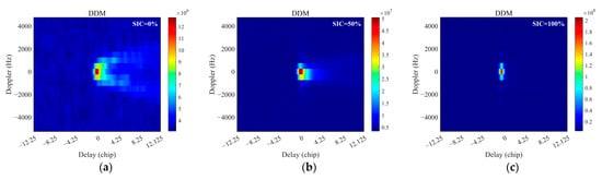
Figure 1.
DDM under different SICs: (a) DDM for a SIC of 0%, (b) DDM for a SIC of 50%, (c) DDM for a SIC of 100%.
3.3. Feature Extraction
The present research identifies six feature parameters [25] from the DDM that are closely associated with SIC, as outlined in the following section:
- 1.
- Power Ratio (PR)The sum of the powers in a 3 × 3 pixel area around the peak power’s delay and Doppler bins, divided by the total power of the entire DDM.
- 2.
- Delay Doppler Average (DDMA):The average power in a 3 × 3 pixel area around the peak power’s delay and Doppler bins.
- 3.
- Equivalent Reflectivity (Γ):Derived from the radar equation and expressed as
- 4.
- Signal-to-Noise Ratio (SNR):The ratio of the average signal power in the delay Doppler region around the DDM peak to the average noise power in the no-signal area of the DDM. The specific calculation is given by the following formula:
- 5.
- Kurtosis (K):Generally, sea ice exhibits higher kurtosis compared to seawater. As SIC increases, power becomes more focused at the specular reflection point, resulting in a higher kurtosis value.
- 6.
- Skewness (S):The skewness observed in the DDM differs between sea ice and seawater. The direction of skewness varies between the two, reflecting differences in surface roughness and scattering characteristics.
Several of these parameters, including SNR, K, S, and Γ, can be directly derived from the GNSS-R L1 data of the FY-3E satellite.
To assess the applicability of these parameters, this study compares their distribution with the reference SIC for a specific day within the corresponding month. The results indicate that the distribution of these parameter values exhibits the same variation with the SIC.
Γ can effectively characterize surface coherence, which is closely related to SIC. PR varies with SIC. Similarly, the DDMA is linked to the scattering power distribution. The SNR is influenced by sea surface roughness. Due to the greater stability of sea ice surfaces under wind forcing compared to open water areas, their reflected signals demonstrate more concentrated patterns (with smaller SNR fluctuations), whereas wind-roughened water surfaces with wave disturbances generate more scattered reflections (showing significant SNR variations). This characteristic divergence establishes SNR as an effective discriminant parameter for SIC retrieval. Therefore, these selected parameters are all related to SIC and can be utilized for its retrieval.
Given the distinct effective scattering areas (ESA) among the BDS, GPS, and Galileo constellations [51], as shown in Figure 2, our model incorporates constellation-specific signal discrimination for GPS, BDS, and Galileo reflections during the training phase [52]. Furthermore, accounting for both hemispheric disparities between Arctic and Antarctic regions and monthly variations in sea ice characteristics, we implement a multi-tiered quality control framework when selecting monthly input features for model training. This systematic process employs parameter-specific thresholds for signal-to-noise ratio (SNR), waveform kurtosis (K), skewness (S), and surface reflectivity (Γ) to identify and remove outliers, thereby ensuring optimal feature parameter selection aligned with seasonal sea ice dynamics. Figure 3 shows the framework for Two-Stage Retrieval.

Figure 2.
DDM of reflected signals from different GNSS constellations: (a) DDM of reflected signals of GPS, (b) DDM of reflected signals of BDS, (c) DDM of reflected signals GALILEO.


Figure 3.
Framework for Two-Stage Retrieval of Sea Ice Concentration via Prior Classification and RF-Based Regression. (a) Step 1: Sea ice detection. (b) Step 2: Develop a Model for Multi-GNSS System Discrimination and Rolling-Window Prediction.
Without prior regional delineation, non-zero SIC values were occasionally observed in typically open-water areas near the Norwegian Sea in the Arctic. Such anomalies are likely associated with calm sea conditions, under which smooth open-water surfaces may exhibit scattering characteristics similar to those of sea ice, leading to false ice detections. To mitigate this issue, a prior regional delineation was introduced to constrain areas that are persistently ice-free, effectively suppressing spurious SIC retrievals in the Arctic open-water regions. As a result, the retrieval accuracy in the Arctic was improved, with the RMSE reduced by 0.0186. In the Antarctic region, the introduction of this prior delineation also led to a notable improvement in retrieval accuracy, with the RMSE reduced by 0.0458.
DDM feature parameters are utilized as model input variables in this study, and a spatiotemporal matching strategy is adopted to align them with the reference SIC product. Each FY-3E GNOS-II L1 observation is spatially matched with the corresponding daily reference Sea Ice Concentration product for the same calendar day. Given that this temporal matching strategy is commonly adopted in sea ice validation studies, this approach represents a justified and standard practice. To address spatial resolution discrepancies between GNSS-R specular points and the passive microwave SIC grid, a bilinear interpolation algorithm was applied to derive corresponding SIC reference data for each specular point. The processed dataset establishes mappings between feature parameters and reference data, providing spatially consistent data for the regression model. Based on the comparative validation using the two reference datasets, the differences in monthly averaged performance metrics over the one-year testing period are relatively small. Specifically, the differences in RMSE between the OSI SAF and NSIDC validations are 0.0089 for the Arctic and 0.0004 for the Antarctic, while the corresponding differences in correlation coefficient (R) are 0.0022 and 0.0036, respectively. These small discrepancies indicate a high level of consistency and stability of the proposed method across different reference datasets. In the following section, we will analyze the use of OSI SAF SIC as the reference data.
Figure 4 clearly shows that the variation trends of the parameter reflectivity in summer and winter differ significantly, indicating a strong seasonal pattern. To evaluate the model’s generalization capability and predictive accuracy, a rolling training-validation scheme was implemented for dataset partitioning. The monthly data were systematically divided into two segments: the first segment served as the training set, while the subsequent segment was reserved for testing. For example, the November 2023 dataset was split into two halves, with the first half used for model training and the second half for validation. This rolling approach [53] was then applied iteratively, where the second half of November’s data became the training set for the first half of December, and so forth.

Figure 4.
(a)The average trend and point distribution of parameter reflectivity of GPS, BDS and GAL systems with SIC in August 2023. (b) The average trend and point distribution of parameter reflectivity of GPS, BDS and GAL systems with SIC in April 2024.
4. Model
Random Forest Regression (RFR)
The Random Forest Regression algorithm is employed to establish an inversion model, through which feature parameters derived from DDMs are systematically mapped to SIC values. As an ensemble learning-based regression method, Random Forest combines multiple decision trees and aggregates their predictions, effectively integrating Bootstrap Aggregation (Bagging) with random feature subspace selection. This mechanism captures complex nonlinear relationships while maintaining low model variance, exhibits strong robustness to high-dimensional features, and is particularly suitable for spaceborne GNSS-R observation scenarios where sea ice monitoring data are limited and feature dimensions are relatively high.
Given the training set {(x1, y1), …, (xn, yn)}, where xj represents the feature vector extracted from the DDM and yj denotes the corresponding SIC value, the Random Forest generates B regression trees {Tb(x)} and averages their outputs to form the final regression function:
Each decision tree Tb is trained on a bootstrap sample drawn with replacement from the original data, and at each node split, only a randomly selected subset of features is considered. This process significantly enhances the model’s generalization ability and suppresses overfitting.
Considering the complex nonlinear relationship between SIC and DDM scattering characteristics—which is influenced by the coupled effects of sea surface temperature, wind turbulence, ocean currents, and other physical processes—this study adopts a Random Forest Regression model. Instead of relying on an explicit kernel mapping, the model automatically learns the interactions between these features through its branching structure, establishing the relationship between SIC and scattering features. Additionally, by optimizing node-splitting criteria (such as mean squared error reduction) and adjusting hyperparameters (e.g., number of trees, tree depth), the model controls its complexity, ensuring high-precision SIC inversion even with limited samples. Furthermore, the feature importance evaluation helps identify key scattering characteristics that significantly impact SIC estimation, providing insight into the main factors driving changes in sea ice conditions.
The evaluation metrics used in the paper are the correlation coefficient (R), Mean Absolute Error (MAE), and Root Mean Squared Error (RMSE). Their calculation formulas are as follows:
In the formulas, n represents the number of samples, is the predicted SIC value for the i-th sample, and is the corresponding reference SIC value.
5. Results
The strategy in this study ensures temporal independence between training and testing datasets within each cycle, facilitating effective model learning while maintaining robust evaluation metrics. This approach dynamically updates model parameters through continuous adaptation, effectively mitigating output deviations caused by seasonal transitions and climatic variations while maintaining precise tracking of environmental parameters. The study period spans from May 2023 to April 2024, covering a full year, with a total of 23 rolling periods.
Furthermore, to account for the distinct characteristics of polar regions—where extensive areas exhibit either high Sea Ice Concentration (SIC > 85%) or open water (SIC < 15%)—the study excluded these extreme values. This targeted analysis focused on the ice-water transition zone, enabling a more accurate evaluation of the model’s performance in dynamic boundary regions.
5.1. Evaluation of SIC Retrieval Accuracy in the Arctic and Antarctic
The monthly performance evaluation aims to assess the overall effectiveness of the retrieval method at the monthly scale. All spatiotemporally matched daily data pairs within the target month are combined to form the evaluation dataset, based on which the monthly error statistics are calculated. For visualization, the monthly maps are generated by directly plotting all valid daily retrieval results within the month at the native spatial resolution of the daily reference product. No temporal averaging or additional weighting is applied. These maps are intended to illustrate the intra-monthly spatial variability of sea ice conditions rather than to represent a statistical monthly mean field.
Based on this comprehensive dataset, the retrieved SIC results (ranging from 0 to 100%) were compared and assessed for accuracy in both the Arctic and Antarctic regions. Figure 5 and Figure 6 present the R and RMSE of the retrieved SIC over a one-year period in the Arctic and Antarctic, respectively, based on two independent reference datasets. To demonstrate the method’s performance across the full range of sea ice conditions, specific months were selected for detailed visualization: during summer, samples with SIC below 80% are more prevalent in both hemispheres, while winter months are predominantly characterized by SIC above 80%. Therefore, Figure 7 and Figure 8 present the predicted top-view Sea Ice Concentration distribution in the Northern and Southern Hemispheres for July 2023 and February 2024, respectively. Table 1 shows the overall results. The comparison of results indicates that, despite the differences between the Antarctic and Arctic regions, the inversion results for most areas each month are close to the reference values, showing good consistency. The monthly SIC results for the Arctic and Antarctic regions using NSIDC Sea Ice Concentration datasets as reference can be found in Appendix A, Table A1. For clarity, the following analysis is conducted using the OSI SAF SIC dataset as the reference.

Figure 5.
The correlation coefficient between retrieved SIC and the OSI SAF and NSIDC reference SIC datasets for the Arctic and Antarctic in the testing set from May 2023 to April 2024.

Figure 6.
The RMSE between retrieved SIC and the OSI SAF and NSIDC reference SIC datasets for the Arctic and Antarctic in the testing set from May 2023 to April 2024.


Figure 7.
(a) Predicted results of the SIC in the testing sets in the Arctic (left), reference data (middle), and their differences (right) in July 2023. (b) Predicted results of the SIC in the testing sets in the Arctic (left), reference data (middle), and their differences (right) in February 2024.

Figure 8.
(a) Predicted results of the SIC in the testing sets in the Antarctic (left), reference data (middle), and their differences (right) in July 2023. (b) Predicted results of the SIC in the testing sets in the Antarctic (left), reference data (middle), and their differences (right) in February 2024.

Table 1.
Results of the SIC for the Arctic and Antarctic regions using NSIDC reference data.
5.1.1. Arctic SIC Retrieval: Accuracy Evaluation
From the time series analysis of rolling test results (Table 1), the prediction accuracy of SIC in the Arctic region exhibited phased stability from May 2023 to April 2024. Except for a significant outlier in September 2023 (R = 0.8796), the R values in other periods remained above 0.9, demonstrating robust model performance under typical seasonal conditions. The sharp decline in September 2023 may be attributed to unpredictable ice-edge variability during the transition from summer melting to autumn freezing, where rapid ice formation or transient polynya dynamics could challenge model parameterization. However, the model showed rapid recovery, with R values rebounding by October 2023, indicating effective adaptation to dynamic environmental changes.
During the spring melt period (March–April 2024), despite increasing thermodynamic instability, the model maintained high accuracy, with R values stabilizing between 0.9617 and 0.9581 and RMSE below 0.1313. This highlights its capability to capture both gradual melt processes and abrupt ice-floe disintegration events.
Compared to traditional single-step retrieval methods, the prior sea ice detection framework proposed in this study effectively addressed the persistent overestimation issue in pure seawater regions, such as open-water areas near the Norwegian Sea. Future research could focus on optimizing input features or refining model architecture, particularly for predictions during September and the period of the early freezing season, to further enhance model stability and accuracy.
5.1.2. Antarctic SIC Retrieval: Accuracy Evaluation
In the Antarctic region, the unique geographical pattern consists of an ice sheet at the core, surrounded by seawater. The presence of a large amount of seawater data could potentially impact the model’s generalization ability. Therefore, in this study, data from latitudes south of 55°S were selected for training and testing.
From the rolling test spanning May 2023 to April 2024, the Antarctic SIC prediction model demonstrated high baseline accuracy during the ice growth period (May–October), achieving exceptional performance (R = 0.9818–0.9854, RMSE = 0.0709–0.0814) and effectively capturing thermodynamically driven ice growth patterns under seasonal radiative cooling (Figure 5 and Figure 6). As the melt season began in November, a sudden rise in accuracy followed by a steady decline indicated the model’s sensitivity to the seasonal retreat of Antarctic sea ice. Notably, the model exhibited rapid seasonal recalibration capability during April 2024, with R values rebounding sharply from 0.8986 in February to 0.9767, accompanied by an RMSE reduction to 0.0755. Overall, Antarctic SIC predictions exhibited stable tendency, with the model effectively capturing the dynamic changes in sea ice and showcasing strong adaptability and generalization capabilities.
5.2. Evaluation of Arctic and Antarctic Ice–Water Transition Zone SIC Retrieval Accuracy
The dataset employed in this study encompasses a wide range of SIC values, including extreme cases of high-density ice (SIC > 85%) and open water (SIC < 15%). To specifically evaluate model performance under dynamic boundary conditions, we constructed a specialized dataset for the ice–water transition zone (SIC = 15–85%) and conducted SIC retrieval.
The dynamic variations in SIC within the ice-water transition zone significantly increase prediction complexity. Analysis of the spatial distribution maps and accuracy evaluation metrics reveals that in the Arctic region as shown in Figure 9 and Table 2, the Arctic ice-water transition zones exhibit higher RMSE values (mean 0.14), peaking at 0.1611 in September due to microwave signal confusion between thin ice and sea water during summer melt season. In contrast, the Antarctic shows significant seasonal variation, with the highest RMSE (0.1690 in February) driven by fragmented ice interference during summer melt, while its rapid model adaptation in winter highlights superior performance in capturing stable ice cover characteristics as shown in Figure 10 and Table 2, particularly excelling throughout the autumn and into the winter sea ice expansion period, which confirms its robust representation of thermodynamics-dominated mechanisms. To address prediction challenges under complex ice conditions, future work could integrate multisource auxiliary data (e.g., Sea Surface Temperature (SST), windspeed) and implement model architecture optimization strategies to further improve retrieval accuracy.

Figure 9.
(a) Results of the SIC for the test set in the Arctic ice-water transition zone (left), reference data (middle), and their differences (right) in July 2023. (b) Results of the SIC for the test set in the Arctic ice-water transition zone (left), reference data (middle), and their differences (right) in February 2024.
Table 2.
Results of SIC in the Arctic and Antarctic ice–water transition zones.

Figure 10.
(a) Results of the SIC for the test set in the Antarctic ice-water transition zone (left), reference data (middle), and their differences (right) in July 2023. (b) Results of the SIC for the test set in the Antarctic ice-water transition zone (left), reference data (middle), and their differences (right) in February 2024.
5.3. Feature Importance
In Random Forest, each tree is trained using bootstrap sampling, meaning that approximately one-third of the data is not used in the training of each tree. This portion of data is referred to as the out-of-bag (OOB) data. To compute the OOB importance, for each tree, we first evaluate the model’s performance—accuracy for classification problems or error for regression problems—using the OOB data. Then, we randomly permute the values of a specific feature and recompute the performance metric. The importance of that feature is defined as the average decrease in accuracy or increase in error before and after the permutation. A larger decrease indicates a more important feature.
The OOB importance measure is highly robust, as it is based on the change in model performance on unseen OOB data. In the accompanying Figure 11, we present the importance values of each feature using a horizontal bar chart, sorted from top to bottom. As shown in Figure 11, specular reflectivity is the paramount parameter for predicting Sea Ice Concentration. The presence of sea ice significantly alters the specular scattering characteristics of the sea surface, thereby directly affecting the reflectivity of GNSS-R signals. However, the discriminative utility of this parameter is modulated by a range of environmental factors. As illustrated in Figure 4, the reflectivity of open water is highly variable: under wind–wave conditions, it can decrease below that of certain thin ice types, complicating accurate retrieval. Furthermore, different ice categories—such as multi-year ice and first-year ice—display overlapping reflectivity signatures owing to distinct internal structures, attenuation properties, and scattering behaviors. Critically, the physical state of sea ice evolves markedly between melting and freezing phases, which induces further shifts in its reflective characteristics. Consequently, the use of reflectivity as a retrieval parameter requires careful consideration of these influences.

Figure 11.
OOB Importance Score of DDM parameters.
6. Discussion
The present study highlights the substantial capabilities of GNSS-R technology for SIC estimation in polar regions. In comparison with traditional remote sensing methods, GNSS-R technology exhibits three significant advantages: global coverage, all-weather observational capacity, and cost-effective synchronous bipolar monitoring via a single satellite platform. Validation against the OSI SAF SIC reference dataset demonstrates the method’s robustness in characterizing stable sea ice distributions. During the respective freezing periods—May to October in the Antarctic and November to April in the Arctic, the technique exhibits strong performance, achieving high consistency in the Arctic (R = 0.95–0.96), and low estimation errors in the Antarctic (RMSE = 0.07–0.08), thereby indicating effective adaptability to seasonal transitions.
Three primary limitations warrant attention: First, accuracy variations emerge under intensified dynamic-thermodynamic coupling across different ice phases. Second, persistent errors in ice-water transition zones reflect unresolved challenges in characterizing dynamic ice margins. Third, frequent ice shelf calving events and extreme polar environmental dynamics (e.g., wind-driven ice advection, abrupt snowfall) may induce localized abrupt errors. To address these issues, future enhancements should prioritize the holistic integration of sea surface environmental factors, particularly by incorporating auxiliary parameters (e.g., SST, wind speed) to strengthen coherence analysis between sea ice dynamics and marine environmental variables. Although current SNR-based filtering effectively preserves most FY-3E observations, developing trajectory-specific denoising algorithms would further minimize manual intervention and optimize processing efficiency.
7. Conclusions
For the first time, this investigation demonstrates the FY-3E mission’s GNOS-II GNSS-R technology as a novel and effective approach for the quantitative retrieval of SIC across both polar regions. Building upon prior region segmentation and adaptive dynamic thresholding for sea ice detection, an innovative RFR-based inversion framework is introduced, which differentiates multi-GNSS signals (GPS, BDS, and Galileo) and integrates a biweekly rolling-window training strategy. Additionally, a comprehensive analysis of DDM scattering characteristics is conducted, strategically extracting and combining key feature parameters to select the most SIC-sensitive parameter set for enhanced retrieval accuracy. However, this framework enables the generation of SIC estimates at the native GNSS-R observation scale (approximately 1 × 6 km), with each estimate corresponding to an individual GNSS-R observation time; owing to the limited daily spatial coverage, the retrieved SIC results are presented at monthly composites for spatial distribution analysis. Large-scale validation demonstrates reliable accuracy, with mean Arctic correlations (R = 0.9450, RMSE = 0.1262) and Antarctic performance (R = 0.9602, RMSE = 0.0818). The biweekly rolling RFR training strategy successfully captures temporal variability, while quantitative error analysis in transition zones provides new insights into GNSS-R scattering mechanisms. Strong consistency with OSI SAF SSMIS products confirms methodological validity. Future efforts will focus on (1) refining ice-water classification algorithms, (2) optimizing SIC inversion for ice-dominated areas, and (3) integrating environmental variables to enhance retrieval robustness. The utilization of FY-3E GNSS-R technology in sea ice monitoring demonstrates great potential, making it a promising avenue for further exploration and advancement.
Author Contributions
Conceptualization, T.X. and C.Y.; methodology, T.X., C.Y., F.H., J.X., W.B. and Q.D.; investigation, T.X.; data curation, X.Z.; writing—original draft preparation, T.X.; writing—review and editing, T.X. and C.Y.; visualization, T.X.; supervision, W.B. and Y.S.; project administration, B.W.; funding acquisition, D.S. All authors have read and agreed to the published version of the manuscript.
Funding
This work was supported by the Key Program of Joint Fund of the National Natural Science Foundation of China and Shandong Province under Grant U22A20586, in part by the Natural Science Foundation of Shandong Province under Grant ZR2022MD015, in part by the Fundamental Research Funds for the Central Universities under Grant 24CX02030A, in part by the Youth Cross Team Scientific Research Project of the Chinese Academy of Sciences under Grant JCTD-2021-10, and in part by the FengYun Application Pioneering Project under Grant FY-APP-2022.0108.
Data Availability Statement
The data presented in this study were obtained from third-party sources. The raw FY-3E GNOS-II data were obtained from the National Satellite Meteorological Center (NSMC) of China and are available at https://satellite.nsmc.org.cn (accessed on 9 March 2025). The ECMWF ERA5 reanalysis data were obtained from the Copernicus Climate Change Service (C3S) Climate Data Store and are available at https://cds.climate.copernicus.eu (accessed on 5 May 2025). The OSI SAF sea ice concentration reference data were obtained from the EUMETSAT Ocean and Sea Ice Satellite Application Facility and are available at https://osi-saf.eumetsat.int (accessed on 15 April 2025). The Sea Ice Concentrations derived from Nimbus-7 SMMR and DMSP SSM/I-SSMIS passive microwave data (NSIDC-0051, Version 2) were obtained from the NASA National Snow and Ice Data Center (NSIDC) and are available at https://nsidc.org/data/nsidc-0051/versions/2 (accessed on 24 December 2025).
Acknowledgments
The authors would like to acknowledge Copernicus Climate Change Service for providing the ECMWF ERA5 reanalysis data, OSI SAF for providing the Sea Ice Concentration data, and the National Snow and Ice Data Center (NSIDC) for providing the Sea Ice Concentration products derived from Nimbus-7 SMMR and DMSP SSM/I–SSMIS passive microwave observations.
Conflicts of Interest
The authors declare no conflicts of interest.
Appendix A
Table A1.
Results of SIC for the Arctic and Antarctic regions using NSIDC reference data.
Table A1.
Results of SIC for the Arctic and Antarctic regions using NSIDC reference data.
| Month | Arctic | Antarctic | ||||
|---|---|---|---|---|---|---|
| R | RMSE | MAE | R | RMSE | MAE | |
| May 2023 | 0.9605 | 0.1233 | 0.0583 | 0.9805 | 0.0697 | 0.0228 |
| June 2023 | 0.9404 | 0.1430 | 0.0776 | 0.9804 | 0.0737 | 0.0269 |
| July 2023 | 0.923 | 0.1247 | 0.0581 | 0.9786 | 0.0809 | 0.0324 |
| August 2023 | 0.8804 | 0.1118 | 0.0450 | 0.9828 | 0.0724 | 0.0288 |
| September 2023 | 0.8963 | 0.1031 | 0.0355 | 0.9768 | 0.0815 | 0.0337 |
| October 2023 | 0.9556 | 0.1151 | 0.0553 | 0.9813 | 0.0744 | 0.0301 |
| November 2023 | 0.9706 | 0.1119 | 0.0515 | 0.9211 | 0.1356 | 0.0535 |
| December 2023 | 0.9678 | 0.1152 | 0.0500 | 0.9328 | 0.1024 | 0.0369 |
| January 2024 | 0.9753 | 0.1032 | 0.0450 | 0.9070 | 0.0862 | 0.0223 |
| February 2024 | 0.9637 | 0.1191 | 0.0551 | 0.9099 | 0.0749 | 0.0178 |
| March 2024 | 0.9636 | 0.1225 | 0.0547 | 0.9502 | 0.0688 | 0.0174 |
| April 2024 | 0.9700 | 0.1146 | 0.0453 | 0.9782 | 0.0663 | 0.0293 |
| Average | 0.9473 | 0.1173 | 0.0527 | 0.9566 | 0.0822 | 0.0293 |
References
- Wang, X.D.; Wu, Z.K. Variability in Polar Sea Ice (1989–2018). IEEE Geosci. Remote Sens. Lett. 2021, 18, 1520–1524. [Google Scholar] [CrossRef]
- Peng, G.; Meier, W.N. Characterization of a Satellite-Based Passive Microwave Sea Ice Concentration Climate Data Record. In Proceedings of the 2013 IEEE International Geoscience and Remote Sensing Symposium (IGARSS), Melbourne, Australia, 21–26 July 2013; pp. 232–235. [Google Scholar] [CrossRef]
- Stroeve, J.C.; Serreze, M.C.; Holland, M.M.; Kay, J.E.; Malanik, J.; Barrett, A.P. The Arctic’s rapidly shrinking sea ice cover: A research synthesis. Clim. Change 2012, 110, 1005–1027. [Google Scholar] [CrossRef]
- Lin, B.; Zheng, M.; Chu, X.; Mao, W.; Zhang, D.; Zhang, M. An overview of scholarly literature on navigation hazards in Arctic shipping routes. Environ. Sci. Pollut. Res. 2024, 31, 40419–40435. [Google Scholar] [CrossRef]
- Comiso, J.C.; Cavalieri, D.J.; Parkinson, C.L.; Gloersen, P. Passive microwave algorithms for sea ice concentration: A comparison of two techniques. Remote Sens. Environ. 1997, 60, 357–384. [Google Scholar] [CrossRef]
- Qu, Z.F.; Su, J. Improved algorithm for determining the freeze onset of Arctic sea ice using AMSR-E/2 data. Remote Sens. Environ. 2023, 297, 113748. [Google Scholar] [CrossRef]
- Qu, M.; Lei, R.B.; Liu, Y.; Li, N. Arctic Sea ice leads detected using sentinel-1B SAR image and their responses to atmosphere circulation and sea ice dynamics. Remote Sens. Environ. 2024, 308, 114193. [Google Scholar] [CrossRef]
- Mäkynen, M.; Karvonen, J. MODIS sea ice thickness and open water–sea ice charts over the Barents and Kara seas for development and validation of sea ice products from microwave sensor data. Remote Sens. 2017, 9, 1324. [Google Scholar] [CrossRef]
- Soulat, F.; Caparrini, M.; Germain, O.; Lopez-Dekker, P.; Taani, M.; Ruffini, G. Sea state monitoring using coastal GNSS-R. Geophys. Res. Lett. 2004, 31, L21303. [Google Scholar] [CrossRef]
- Guo, W.F.; Du, H.; Cheong, J.W.; Southwell, B.J.; Dempster, A.G. GNSS-R Wind Speed Retrieval of Sea Surface Based on Particle Swarm Optimization Algorithm. IEEE Trans. Geosci. Remote Sens. 2022, 60, 4202414. [Google Scholar] [CrossRef]
- Clarizia, M.P.; Ruf, C.S.; Jales, P.; Gommenginger, C. Spaceborne GNSS-R Minimum Variance Wind Speed Estimator. IEEE Trans. Geosci. Remote Sens. 2014, 52, 6829–6843. [Google Scholar] [CrossRef]
- Camps, A.; Park, H.; Pablos, M.; Foti, G.; Gommenginger, C.P.; Liu, P.W.; Judge, J. Sensitivity of GNSS-R Spaceborne Observations to Soil Moisture and Vegetation. IEEE J. Sel. Top. Appl. Earth Obs. Remote Sens. 2016, 9, 4730–4742. [Google Scholar] [CrossRef]
- Wu, X.R.; Ma, W.X.; Xia, J.M.; Bai, W.H.; Jin, S.G.; Calabia, A. Spaceborne GNSS-R Soil Moisture Retrieval: Status, Development Opportunities, and Challenges. Remote Sens. 2021, 13, 45. [Google Scholar] [CrossRef]
- Yang, C.Z.; Mao, K.B.; Guo, Z.H.; Shi, J.C.; Bateni, S.M.; Yuan, Z.J. Review of GNSS-R Technology for Soil Moisture Inversion. Remote Sens. 2024, 16, 1193. [Google Scholar] [CrossRef]
- Hu, Y.; Yuan, X.T.; Liu, W.; Wickert, J.; Jiang, Z.H. GNSS-R Snow Depth Inversion Based on Variational Mode Decomposition With Multi-GNSS Constellations. IEEE Trans. Geosci. Remote Sens. 2022, 60, 2005512. [Google Scholar] [CrossRef]
- Yu, K.; Wang, S.; Li, Y.; Chang, X.; Li, J. Snow depth estimation with GNSS-R dual receiver observation. Remote Sens. 2019, 11, 2056. [Google Scholar] [CrossRef]
- Yan, Q.Y.; Huang, W.M. Sea Ice Remote Sensing Using GNSS-R: A Review. Remote Sens. 2019, 11, 2565. [Google Scholar] [CrossRef]
- Alonso-Arroyo, A.; Camps, A.; Monerris, A.; Rüdiger, C.; Walker, J.P.; Onrubia, R.; Querol, J.; Park, H.; Pascual, D. On the correlation between GNSS-R reflectivity and L-band microwave radiometry. IEEE J. Sel. Top. Appl. Earth Obs. Remote Sens. 2016, 9, 5862–5879. [Google Scholar] [CrossRef]
- Llaveria, D.; Munoz-Martin, J.F.; Herbert, C.; Pablos, M.; Park, H.; Camps, A. Sea Ice Concentration and Sea Ice Extent Mapping with L-Band Microwave Radiometry and GNSS-R Data from the FFSCat Mission Using Neural Networks. Remote Sens. 2021, 13, 1139. [Google Scholar] [CrossRef]
- Buendía, R.N.; Tabibi, S.; Talpe, M.; Otosaka, I. Ice sheet height retrievals from Spire grazing angle GNSS-R. Remote Sens. Environ. 2023, 297, 113757. [Google Scholar] [CrossRef]
- Yan, Q.Y.; Huang, W.M.; Foti, G. Quantification of the Relationship Between Sea Surface Roughness and the Size of the Glistening Zone for GNSS-R. IEEE Geosci. Remote Sens. Lett. 2018, 15, 237–241. [Google Scholar] [CrossRef]
- Camps, A. Spatial Resolution in GNSS-R Under Coherent Scattering. IEEE Geosci. Remote Sens. Lett. 2020, 17, 32–36. [Google Scholar] [CrossRef]
- Bu, J.W.; Liu, X.Y.; Wang, Q.L.; Li, L.H.; Zuo, X.Q.; Yu, K.G.; Huang, W.M. Ocean Remote Sensing Using Spaceborne GNSS-Reflectometry: A Review. IEEE J. Sel. Top. Appl. Earth Obs. Remote Sens. 2024, 17, 13047–13076. [Google Scholar] [CrossRef]
- Strandberg, J.; Hobiger, T.; Haas, R. Coastal Sea Ice Detection Using Ground-Based GNSS-R. IEEE Geosci. Remote Sens. Lett. 2017, 14, 1552–1556. [Google Scholar] [CrossRef]
- Zhu, Y.C.; Tao, T.Y.; Yu, K.G.; Li, Z.X.; Qu, X.C.; Ye, Z.R.; Geng, J.; Zou, J.G.; Semmling, M.; Wickert, J. Sensing Sea Ice Based on Doppler Spread Analysis of Spaceborne GNSS-R Data. IEEE J. Sel. Top. Appl. Earth Obs. Remote Sens. 2020, 13, 217–226. [Google Scholar] [CrossRef]
- Yan, Q.Y.; Huang, W.M. Sea Ice Sensing From GNSS-R Data Using Convolutional Neural Networks. IEEE Geosci. Remote Sens. Lett. 2018, 15, 1510–1514. [Google Scholar] [CrossRef]
- Sun, Y.Q.; Huang, F.X.; Xia, J.M.; Yin, C.; Bai, W.H.; Du, Q.F.; Wang, X.Y.; Cai, Y.R.; Li, W.; Yang, G.L.; et al. GNOS-II on Fengyun-3 Satellite Series: Exploration of Multi-GNSS Reflection Signals for Operational Applications. Remote Sens. 2023, 15, 5756. [Google Scholar] [CrossRef]
- Rodriguez-Alvarez, N.; Holt, B.; Jaruwatanadilok, S.; Podest, E.; Cavanaugh, K.C. An Arctic sea ice multi-step classification based on GNSS-R data from the TDS-1 mission. Remote Sens. Environ. 2019, 230, 111202. [Google Scholar] [CrossRef]
- Yan, Q.Y.; Huang, W.M. Sea Ice Thickness Measurement Using Spaceborne GNSS-R: First Results with TechDemoSat-1 Data. IEEE J. Sel. Top. Appl. Earth Obs. Remote Sens. 2020, 13, 577–587. [Google Scholar] [CrossRef]
- Zhu, Y.C.; Tao, T.Y.; Li, J.Y.; Yu, K.G.; Wang, L.; Qu, X.C.; Li, S.P.; Semmling, M.; Wickert, J. Spaceborne GNSS-R for Sea Ice Classification Using Machine Learning Classifiers. Remote Sens. 2021, 13, 4577. [Google Scholar] [CrossRef]
- Semmling, A.M.; Rosel, A.; Divine, D.V.; Gerland, S.; Stienne, G.; Reboul, S.; Ludwig, M.; Wickert, J.; Schuh, H. Sea-Ice Concentration Derived from GNSS Reflection Measurements in Fram Strait. IEEE Trans. Geosci. Remote Sens. 2019, 57, 10350–10361. [Google Scholar] [CrossRef]
- Foti, G.; Gommenginger, C.; Srokosz, M. First Spaceborne GNSS-Reflectometry Observations of Hurricanes from the UK TechDemoSat-1 Mission. Geophys. Res. Lett. 2017, 44, 12358–12366. [Google Scholar] [CrossRef]
- Yan, Q.Y.; Huang, W.M.; Moloney, C. Neural Networks Based Sea Ice Detection and Concentration Retrieval From GNSS-R Delay-Doppler Maps. IEEE J. Sel. Top. Appl. Earth Obs. Remote Sens. 2017, 10, 3789–3798. [Google Scholar] [CrossRef]
- Zhu, Y.; Tao, T.; Zou, J.; Yu, K.; Wickert, J.; Semmling, M. Spaceborne GNSS Reflectometry for Retrieving Sea Ice Concentration Using TDS-1 Data. IEEE Geosci. Remote Sens. Lett. 2021, 18, 612–616. [Google Scholar] [CrossRef]
- Yang, L.; Guo, B.F.; Zhang, Z.Y.; Zhang, X.F. DNN-Based Retrieval of Arctic Sea Ice Concentration From GNSS-R and Its Effects on the Synoptic-Scale Forecasting as Supplementary Observation Source. Geophys. Res. Lett. 2023, 50, e2023GL104219. [Google Scholar] [CrossRef]
- Ban, W.; Zhang, L.H.; Zhang, X.H.; Nie, H.; Chen, X.L.; Chen, X.J. Wind-Concerned Sea Ice Detection and Concentration Retrieval From GNSS-R Data Using a Modified Convolutional Neural Network. IEEE J. Sel. Top. Appl. Earth Obs. Remote Sens. 2025, 18, 9755–9763. [Google Scholar] [CrossRef]
- Zhang, P.; Hu, X.Q.; Lu, Q.F.; Zhu, A.J.; Lin, M.Y.; Sun, L.; Chen, L.; Xu, N. FY-3E: The First Operational Meteorological Satellite Mission in an Early Morning Orbit. Adv. Atmos. Sci. 2022, 39, 1–8. [Google Scholar] [CrossRef]
- Qiu, T.S.; Wang, X.Y.; Sun, Y.Q.; Li, F.; Wang, Z.Y.; Xia, J.M.; Du, Q.F.; Bai, W.H.; Cai, Y.R.; Wang, D.W.; et al. An Innovative Signal Processing Scheme for Spaceborne Integrated GNSS Remote Sensors. Remote Sens. 2023, 15, 745. [Google Scholar] [CrossRef]
- Sun, Y.; Wang, X.; Du, Q.; Bai, W.; Xia, J.; Cai, Y.; Wang, D.; Wu, C.; Meng, X.; Tian, Y. The status and progress of Fengyun-3E GNOS II mission for GNSS remote sensing. In Proceedings of the 2019 IEEE International Geoscience and Remote Sensing Symposium (IGARSS), Yokohama, Japan, 28 July–2 August 2019; pp. 5181–5184. [Google Scholar] [CrossRef]
- Cui, Z.; Zheng, W.; Wu, F.; Li, X.P.; Zhu, C.; Liu, Z.Q.; Ma, X.F. Improving GNSS-R Sea Surface Altimetry Precision Based on the Novel Dual Circularly Polarized Phased Array Antenna Model. Remote Sens. 2021, 13, 2974. [Google Scholar] [CrossRef]
- Huang, F.; Sun, Y.; Xia, J.; Yin, C.; Bai, W.; Du, Q.; Zhai, X.; Yang, G.; Chen, L.; Lu, W. Progress on the GNSS-R product from Fengyun-3 missions. In Proceedings of the 2024 IEEE International Geoscience and Remote Sensing Symposium (IGARSS), Kuala Lumpur, Malaysia, 7–12 July 2024; pp. 6717–6720. [Google Scholar] [CrossRef]
- Yang, G.; Bai, W.; Wang, J.; Hu, X.; Zhang, P.; Sun, Y.; Xu, N.; Zhai, X.; Xiao, X.; Xia, J. FY3E GNOS II GNSS reflectometry: Mission review and first results. Remote Sens. 2022, 14, 988. [Google Scholar] [CrossRef]
- Lavergne, T.; Down, E. A climate data record of year-round global sea-ice drift from the EUMETSAT Ocean and Sea Ice Satellite Application Facility (OSI SAF). Earth Syst. Sci. Data 2023, 15, 5807–5834. [Google Scholar] [CrossRef]
- Alonso-Arroyo, A.; Zavorotny, V.U.; Camps, A. Sea Ice Detection Using UK TDS-1 GNSS-R Data. IEEE Trans. Geosci. Remote Sens. 2017, 55, 4989–5001. [Google Scholar] [CrossRef]
- Lavergne, T.; Sørensen, A.M.; Kern, S.; Tonboe, R.; Notz, D.; Aaboe, S.; Bell, L.; Dybkjær, G.; Eastwood, S.; Gabarro, C.; et al. Version 2 of the EUMETSAT OSI SAF and ESA CCI sea-ice concentration climate data records. Cryosphere 2019, 13, 49–78. [Google Scholar] [CrossRef]
- Hersbach, H.; Bell, B.; Berrisford, P.; Hirahara, S.; Horányi, A.; Muñoz-Sabater, J.; Nicolas, J.; Peubey, C.; Radu, R.; Schepers, D. The ERA5 global reanalysis. Q. J. R. Meteorol. Soc. 2020, 146, 1999–2049. [Google Scholar] [CrossRef]
- Yan, Q.; Huang, W. Spaceborne GNSS-R Sea Ice Detection Using Delay-Doppler Maps: First Results From the U.K. TechDemoSat-1 Mission. IEEE J. Sel. Top. Appl. Earth Obs. Remote Sens. 2016, 9, 4795–4801. [Google Scholar] [CrossRef]
- Ma, Z.; Camps, A.; Park, H.; Zhang, S.; Li, X.; Wigneron, J.-P. Sensitivity study of multi-constellation GNSS-R to soil moisture and surface roughness using FY-3E GNOS-II data. IEEE J. Sel. Top. Appl. Earth Obs. Remote Sens. 2024, 18, 413–423. [Google Scholar] [CrossRef]
- Zhang, Z.Y.; Guo, B.F.; Nan, Y.; Wu, X.; Du, H.; Li, F.H.; Zhai, J.S. Preliminary Sea Ice Detection Results From GNSS-R Payload on Board Chinese Jilin-1 Wideband-01B (J1-01B) Satellite. IEEE Geosci. Remote Sens. Lett. 2024, 21, 4500405. [Google Scholar] [CrossRef]
- Ma, D.; Gao, Y.; Hou, C.P.; Li, M.L.; Yang, Y. Multi-Task Retrieval of Sea Ice Based on GNSS-R: An Integrated Framework Guided by Semi-Supervised Anomaly Detection. IEEE Access 2024, 12, 181590–181606. [Google Scholar] [CrossRef]
- Yu, H.; Du, Q.; Xia, J.; Huang, F.; Yin, C.; Meng, X.; Bai, W.; Sun, Y.; Wang, X.; Duan, L.; et al. Comparative Analysis of SWH Retrieval Between BDS-R and GPS-R Utilizing FY-3E/GNOS-II Data. IEEE J. Sel. Top. Appl. Earth Obs. Remote Sens. 2025, 18, 6520–6531. [Google Scholar] [CrossRef]
- Zhu, Y.; Guo, F.; Zhang, X. Spaceborne GNSS-R soil moisture retrieval from GPS/BDS-3/Galileo satellites. GPS Sol. 2025, 29, 10. [Google Scholar] [CrossRef]
- Wang, Z.; Zhang, Y.; Fu, H. Autoregressive Prediction with Rolling Mechanism for Time Series Forecasting with Small Sample Size. Math. Probl. Eng. 2014, 2014, 572173. [Google Scholar] [CrossRef]


Disclaimer/Publisher’s Note: The statements, opinions and data contained in all publications are solely those of the individual author(s) and contributor(s) and not of MDPI and/or the editor(s). MDPI and/or the editor(s) disclaim responsibility for any injury to people or property resulting from any ideas, methods, instructions or products referred to in the content. |
© 2026 by the authors. Licensee MDPI, Basel, Switzerland. This article is an open access article distributed under the terms and conditions of the Creative Commons Attribution (CC BY) license.