Highlights
What are the main findings?
- The study presents a novel detector-selection framework that effectively suppresses striping noise in multi-column scanning radiometers by jointly optimizing for inter-detector uniformity (using the proposed IRBTD metric) and sensitivity, achieving a 10–40% reduction in inconsistency with only a 1–4% increase in NEdT.
- The method employs a Viterbi algorithm-based dynamic programming approach to solve the global detector-selection optimization problem with linear time complexity, making it computationally efficient and suitable for potential real-time on-board implementation.
What are the implications of the main findings?
- This source-level suppression approach fundamentally avoids the information loss or distortion associated with image post-processing destriping techniques, thereby preserving the physical authenticity and radiometric consistency of the original observational data.
- The framework provides a generic, calibration-independent enhancement strategy for scanning radiometers with multi-column redundant architectures, offering a practical pathway to improve image quality without modifying existing calibration models or ground processing chains.
Abstract
Striping noise is a common problem in multi-detector scanning radiometers on remote sensing satellites, typically caused by response inconsistency among detector elements. For payloads with a multi-column redundant architecture, this paper proposes a detector-selection framework that jointly considers sensitivity and uniformity from the perspective of detector-element selection to mitigate striping noise. First, the degree of detector consistency is quantified using the Inter-Row Brightness Temperature Difference (IRBTD). Then, a dynamic programming approach based on the Viterbi algorithm is employed to select detector elements row by row with linear time complexity, optimizing the process through a weighted cost function that integrates sensitivity and consistency. Experiments on raw data from the FY-4B Geostationary High-speed Imager (GHI) show that the method reduces inconsistency by 10–40% while increasing the noise-equivalent temperature difference (NEdT) by only 1–4% (≤4 mK). The average IRBTD decreases by approximately 20–100 mK, and high-frequency striping energy is significantly suppressed (reduction of 50–90%). The algorithm exhibits linear time complexity and low computational overhead, making it suitable for real-time on-board processing. Its weighting parameter enables flexible trade-offs between sensitivity and uniformity. By suppressing striping noise directly during the detector-selection stage without introducing data distortion or requiring calibration adjustments, the proposed method can be widely applied to scanning radiometers that employ multi-column long-linear-arrays.
1. Introduction
Striping noise is a common issue in infrared band imaging for remote sensing satellites [1]. For payloads that utilize multi-detector-element linear arrays and perform whiskbroom scanning, this noise primarily originates from inconsistency in the responses among detector elements. Inter-detector consistency describes the degree to which different detector elements produce the same output response when observing an identical target. When the physical quantities retrieved from the same radiance target differ across detector elements, inconsistency occurs, which subsequently manifests as striping noise in the imagery (in staring focal-plane arrays, such inconsistency often appears as isolated noisy pixels). Although radiometric calibration is designed in principle to eliminate these inconsistencies, residual errors frequently persist in practice. Factors contributing to this residual inconsistency include variations in the calibration model fitting accuracy for different detector elements [2], non-uniformity in the spectral response function [3,4,5,6], low-frequency noise [7], and electrical crosstalk [8], among others.
With the continuous improvement in detector sensitivity, the level of random noise has gradually fallen below the error introduced by striping noise, making striping artifacts increasingly conspicuous in imagery, and their impact cannot be overlooked. Specifically, striping can introduce systematic radiometric bias and spatial discontinuities during geometric registration, reprojection, and resampling processes, thereby reducing resampling accuracy and generating spurious structures [9]. Furthermore, striping can obscure or distort genuine features in low-texture regions and near weak boundaries, impairing the accuracy of image classification and target detection [1,10]. In applications sensitive to high temperatures or extreme radiance values—such as hotspot and fire detection—striping, combined with instrument noise, can significantly degrade detection sensitivity [11]. The increase in radiometric bias and variance caused by striping also adversely affects the retrieval accuracy and uncertainty assessment of quantitative products, such as sea surface temperature [12]. Precisely for these reasons, suppressing striping noise is widely regarded as a critical task in satellite data processing standards and product specifications, and enhancing inter-detector consistency has become increasingly important [13,14,15].
Existing methods for correcting striping noise (i.e., inconsistency) can be broadly categorized into two types: calibration-based methods and image-based methods. Calibration-based methods aim to reduce inter-detector errors by refining the calibration model and radiometric correction procedures, though in practice they often struggle to fully eliminate residual inconsistency [16,17]. Image-based methods, on the other hand, apply post-processing directly to the image data, employing techniques such as statistical matching [18], filtering [19], variational optimization [20], and deep learning [21]. While these methods can effectively suppress striping, the image processing inevitably leads to the loss of some original information and may introduce additional distortion. Consequently, many remote sensing satellites users and operational agencies tend to avoid relying solely on image post-processing for striping removal.
In recent years, the infrared bands of new-generation geostationary imagers have widely adopted a multi-column redundant architecture based on large-scale long linear focal plane arrays. Examples include the ABI on the GOES-R series [22], the AHI on Himawari-8/9 [23,24], the AMI on GEO-KOMPSAT-2A [25], the FCI on the MTG platform [26], and the GHI on China’s FY-4B satellite [8]. This architecture arranges identical long linear detector arrays in parallel as multiple columns (typically four or six), enabling them to simultaneously observe the same ground scene. When synthesizing the final remote sensing image, the system selects data from only one optimal detector element per row for image assembly. A schematic of the imaging process is shown in Figure 1. This design not only effectively mitigates the impact of blind detector elements but also significantly enhances data quality.
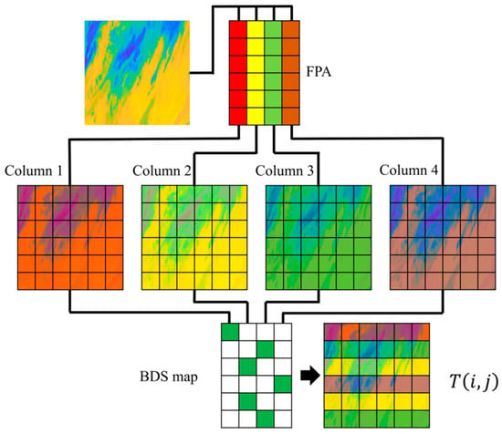
Figure 1.
Schematic diagram of the BDS and image module construction workflow, where different colors indicate different columns of the FPA and the arrows indicate the data flow.
The multi-column redundant architecture provides a new perspective for suppressing striping noise: can the selection strategy of detector elements be optimized to minimize striping noise in the final synthesized image? To date, no research has systematically addressed striping noise suppression from the perspective of detector-element selection. However, utilizing detector selection to improve detector consistency offers unique theoretical and practical value: since all detector elements involved in the synthesis (except for blind ones) are physical measurements of the real scene, this approach essentially performs optimal screening and combination of existing real observational data, rather than transforming or modifying the data values. Consequently, it fundamentally avoids the inevitable information loss or distortion associated with image post-processing, thereby preserving to the greatest extent the physical authenticity and radiometric consistency of the raw observational data. This characteristic is particularly important for high-end applications that rely on original radiance values for quantitative retrieval, long-term time-series analysis, and data assimilation.
From an engineering implementation standpoint, this concept aligns naturally with the existing multi-column redundant hardware architecture and detector-selection workflow, providing a new pathway to enhance image quality without altering the current calibration models or downlink data chains. Therefore, systematically investigating striping noise suppression from the detector-selection perspective holds significant and distinctive research value.
This study takes the infrared band data of FY-4B GHI as an example and proposes a detector-element selection method that strikes a balance between striping noise and detector sensitivity. The method significantly reduces striping noise already at the image-assembly stage, without modifying the existing calibration model or altering the raw detector measurements, and without introducing any image post-processing workflow—thereby avoiding additional physical distortion. The algorithm exhibits low computational complexity and holds potential for real-time on-board implementation.
The main contributions of this work are as follows:
- (1)
- A Source-Level Suppression Framework Based on Detector Selection: To address the limitations of existing calibration and post-processing methods, which may introduce information distortion or complicate engineering deployment, this study proposes a striping noise suppression framework based on optimal detector selection. Without modifying the existing calibration pipeline, the framework effectively suppresses striping noise at its source during the image synthesis stage by intelligently selecting detector data from raw measurements.
- (2)
- Engineering-Oriented Quantitative Metrics: In response to the lack of clear metrics for evaluating in-orbit remote sensing image uniformity and striping noise, this study proposes and adopts the Inter-row Brightness Temperature Difference (IRBTD) as a quantitative indicator to assess inter-detector consistency. This metric provides a clear and reliable basis for defining optimization objectives and evaluating algorithm performance.
- (3)
- An Efficient Solver Based on Viterbi Dynamic Programming: The row-by-row detector selection problem is formulated as a sequential decision-making optimization task. The Viterbi algorithm is introduced to achieve a globally optimal or near-optimal search, reducing the computational complexity to linear scale. This significantly improves processing efficiency, meeting the requirements for speed and stability in offline and near-real-time processing, thereby laying the algorithmic foundation for engineering implementation.
- (4)
- A Tunable Parameter Mechanism for Engineering Trade-offs: A flexible and controllable trade-off between uniformity (IRBTD) and sensitivity (NEdT) is achieved through a weighting coefficient β. Practical guidelines for selecting β based on the “Elbow Method” are provided. Systematic experiments on multi-scene data analyze the impact of β on various performance metrics, demonstrating the method’s strong engineering adaptability and potential for broader application.
The experimental results of this study on FY-4B GHI data indicate that, within an engineering-acceptable range where the NEdT increases by less than 4% on average (1–4 mK), the IRBTD is reduced by 20–100 mK, and high-frequency striping noise energy is decreased by over 50% on average. Both visual comparison and spectral analysis confirm significant suppression of striping noise.
The striping-noise suppression method proposed in this paper is not mutually exclusive with existing destriping approaches; instead, it essentially performs pre-emptive suppression at the detector-selection stage, and can thereafter be seamlessly compatible with or further combined with image post-processing or other techniques. Therefore, the proposed method complements and synergizes with existing methods rather than competing with them.
2. Materials and Methods
2.1. Best Detector Selection
The multi-column redundant detector architecture allows the selection of one “best” detector element from each row of the focal plane to generate the final image—this operation is called Best Detector-element Selection (BDS). The resulting row-index map of the selected detector elements is referred to as the BDS map. For most payloads, the BDS map is determined during pre-launch ground testing and is generally not updated on-orbit to maintain system stability and to avoid the additional risks and costs associated with updates [22]. Payloads such as ABI, AHI, and AMI typically downlink only the data from the selected best detector elements during routine operation, which significantly reduces data volume and downlink burden. In contrast, FY-4B GHI downlinks data from all detector columns and performs image synthesis and post-processing on the ground. This provides an opportunity to study detector-selection strategies in depth. Therefore, this paper uses GHI data to demonstrate the proposed method (Additionally, the raw data from the payload are typically not publicly available to users, while our research team has access to the raw GHI data). The parameters of GHI are listed in Table 1 [8]. Figure 2 shows the four-linear-array observation image from a GHI observation task (Sample 1), where the white horizontal lines indicate blind detector elements.

Table 1.
Main performance parameters of spectral bands of GHI.
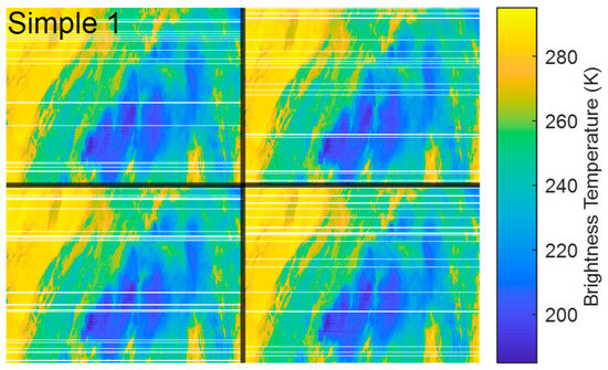
Figure 2.
Raw observation image of Sample 1 from the four detector columns (blind elements are marked by white horizontal lines).
Ideally, the best detector element should exhibit high sensitivity, accurate calibration characteristics, long-term stability, and good inter-detector consistency. However, there is currently no universally accepted evaluation criterion for defining the “best” detector element. Existing BDS maps often prioritize the individual performance of detector elements, such as the sensitivity of a single detector, while giving insufficient consideration to inter-detector consistency. This leads to the frequent appearance of striping noise in the final imagery. For example, the current BDS strategy for GHI selects the detector element with the highest sensitivity (the lowest NEdT) for image assembly. While this approach maximizes the sensitivity of the remote sensing data, it lacks consideration of other metrics such as consistency. As a result, the final assembled images still exhibit a non-negligible level of striping noise. This is illustrated in the sample GHI observation images shown in Figure 3 (Sample 1) and Figure 4 (Sample 2), where regions with pronounced striping are highlighted in enlarged insets.
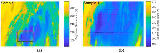
Figure 3.
Remote sensing image of Sample 1 processed by the traditional BDS: (a) full scene; (b) local enlargement of the red box area.
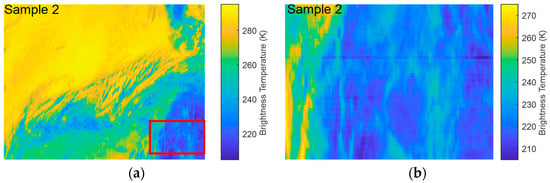
Figure 4.
Remote sensing image of Sample 2 processed by the traditional BDS: (a) full scene; (b) local enlargement of the red box area.
Furthermore, even when attempts are made to account for inter-detector consistency during the selection process, its influencing factors are complex and diverse. It is difficult to conduct comprehensive and precise measurements of these factors during ground testing. Moreover, the relevant characteristics may change after the instrument is in orbit. Consequently, BDS maps determined based on ground testing often struggle to maintain good detector consistency in practical applications.
Some ground systems (e.g., the ground processing chains of ABI and AHI) are capable of monitoring and repairing isolated bad lines on-orbit. When an isolated bad line is detected in a remote sensing image, the system identifies the corresponding detector element in that row as anomalous and further analyzes its calibration coefficients and raw data [2]. If the issue is confirmed to originate from the detector itself, the bad line can be repaired by updating the BDS map to replace the faulty detector element [27]. Although this approach is straightforward and effective, it still has two main limitations: (1) it is primarily suitable for identifying and replacing isolated, clearly abnormal scan lines, but difficult to improve the overall level of striping noise across the entire remote sensing image; (2) the ground-based detection and update process is time-consuming, and once the raw data is corrupted, it cannot be recovered.
Therefore, to effectively enhance image quality, it is necessary to propose a detector-selection method capable of improving striping noise holistically. Moreover, the method should have the potential for real-time on-board processing, thereby avoiding data loss caused by post-facto correction.
2.2. Inter-Row Brightness Temperature Difference
A variety of metrics exist for evaluating striping noise in images, such as peak signal-to-noise ratio, image power spectrum, noise reduction coefficient [28,29], and the streaking metric ratio [30]. Since the remote sensing images processed in this study lack an ideal reference ground truth, it is difficult to directly employ reference-based metrics for effective analysis. Furthermore, as this study aims to suppress striping noise at the level of detector elements, it is necessary to accurately map the observed striping noise to specific detector elements. The streaking metric ratio can, to some extent, meet these requirements. A brief introduction to this method is provided first below.
For an acquired radiance remote sensing image, the average radiance for each row is calculated sequentially. The absolute difference between the current row and the average of its immediately adjacent rows is then determined and divided by the mean radiance of the row itself, yielding the streaking metric ratio for that row. A larger value of this coefficient indicates more pronounced striping noise in the corresponding row and greater inconsistency of the associated detector element. This method has been applied to evaluate detector consistency in the visible band of ABI, and its calculation formula is as follows:
where denotes the streaking metric ratio for the -th row, represents the average radiance of that row, and and are the average radiances of the immediately adjacent rows above and below, respectively.
This method is capable of evaluating detector consistency in actual remote sensing data, but it has certain limitations: the averaging operation may conceal some striping noise. For instance, if part of a row is darker than the adjacent rows while another part is brighter, the streaking metric ratio may fail to accurately identify the inconsistency present in that row. Therefore, it is necessary to improve upon this parameter.
Building upon the streaking metric ratio, this paper proposes an evaluation metric termed Inter-row Brightness Temperature Difference (IRBTD). This metric can more accurately reflect the severity of striping noise in each row of an image and effectively assess the consistency level among different detector elements. A detailed introduction to IRBTD follows.
Assuming that, under a given BDS map, we have acquired remote sensing data—a brightness temperature image denoted as T (for clarity of presentation, brightness temperature data are used here; the method can be equally applied to radiance images, as the underlying principle is entirely the same).
where i and j denote the pixel positions in the image, i.e., the horizontal and vertical coordinates, respectively. The horizontal coordinate i ranges from 1 to the total number of image rows N, and the vertical coordinate j ranges from 1 to the total number of image columns F; F is determined by the observation task and the observation mode.
In the brightness temperature image T, the difference between each pixel and the average brightness temperature of its adjacent rows is given by:
In (3), represents the absolute difference between the brightness temperature at pixel(i,j) and the average brightness temperature of the same column in the adjacent rows above and below. The valid range for i is from 2 to N − 1.
The average brightness temperature difference between row i and its adjacent rows is calculated as:
In (4), IRBTD(i) denotes the IRBTD for row i, expressed in Kelvin. It is evident that different BDS maps produce different IRBTD outcomes.
For Figure 3 and Figure 4, the corresponding IRBTD values are shown in Figure 5. It can be seen that for most detector elements, IRBTD values fluctuate steadily around 1 K, while a few detector elements exhibit significantly higher values. These anomalies appear consistently across both image samples. In Figure 3 and Figure 4, the rows corresponding to these detector elements clearly display inconsistency (manifested as striping noise), indicating that IRBTD serves as a valid metric for characterizing detector uniformity to a certain extent.
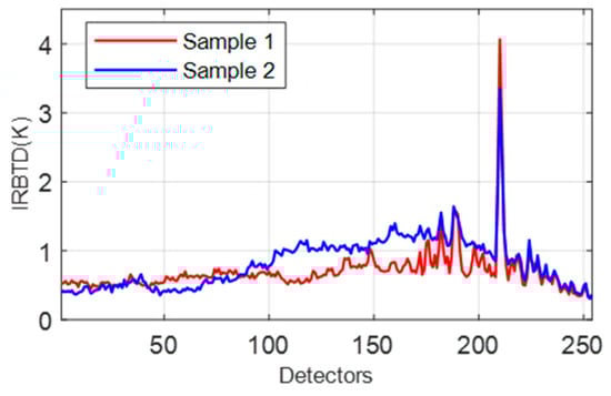
Figure 5.
IRBTD of Sample 1 and Sample 2.
The IRBTD for each detector element consists of three components: the intrinsic inter-row variation in the observed target , the variation caused by detector noise , and the variation due to detector inconsistency (brightness temperature of non-uniformity), as expressed in the following equation
The detector selection method does not influence the target’s intrinsic inter-row variation . Since detector noise is typically small and differences in noise levels across detectors are minimal, the selection method has little effect on . Therefore, the primary influence of the selection method lies in , and thus directly affects IRBTD.
It is worth noting that in scenes such as cloud edges, frontal zones, or areas with abrupt terrain changes, the actual targets observed at corresponding positions in adjacent rows may differ significantly. This leads to an increase in the value of , which in turn causes the IRBTD to rise. Under such conditions, using IRBTD to evaluate detector consistency may result in an overestimation of the degree of inconsistency. However, even in such complex scenes, it remains reasonable to employ IRBTD for assessing the relative strength of consistency among candidate detector elements within the same row of the focal plane: Equation (5) and its physical interpretation still hold. Specifically, although the IRBTD values of all candidate detector elements are generally elevated, comparing their relative magnitudes can still effectively identify detector elements with better consistency, thereby providing a reliable basis for detector-selection decisions. Therefore, for the purpose of detector selection, IRBTD remains applicable even under conditions of highly variable scenes. We will present the processing results for both highly variable and smooth scenes in Results and Discussion.
The average IRBTD across the entire image is calculated as:
Our objective is to determine a BDS map that, after excluding unusable detector elements, selects detector elements with good consistency—specifically by minimizing the average IRBTD—so as to minimize striping noise.
2.3. Detector Selection Based on the Viterbi Algorithm
This section introduces a method for selecting detector elements that optimizes image uniformity. As indicated in (3) and (4), the choice of a detector element in a particular row not only affects the IRBTD(i) for that row but also influences the IRBTD of its adjacent rows, IRBTD(i − 1) and IRBTD(i + 1). These effects can propagate further, impacting uniformity across the entire image. Therefore, the selection problem must be approached holistically, aiming to determine a BDS map that minimizes the overall average IRBTD across all rows.
If brute-force enumeration were used to evaluate all possible selection combinations—and assuming no blind detectors and no elements excluded by sensitivity threshold—the total number of IRBTD computations would be:
This is computationally impractical. To overcome this, we adopt a detector selection approach based on the Viterbi algorithm.
The Viterbi algorithm is a classic dynamic programming technique for determining the most likely sequence of hidden states, widely applied in the field of communications [31]. By reformulating the BDS problem as a shortest-path search, the Viterbi algorithm can be adapted to efficiently compute a globally optimal selection scheme with linear complexity. To illustrate its core concept, we begin with a simplified example.
Consider an Example Matrix (EM) of size N × 4, where i denotes the row index and L denotes the column index. The entries in EM are labeled A, B, C, … up to T; all are positive real numbers, as illustrated in Figure 6. We need to select one entry from each row and compute the absolute difference d between adjacent selected entries. For instance, if the element chosen in the first row is A and in the second row is E, then
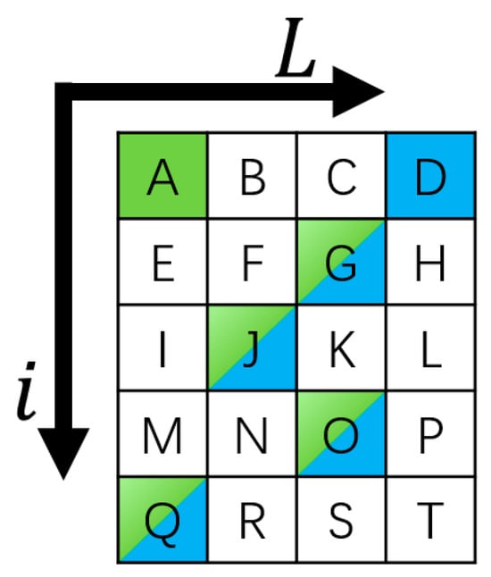
Figure 6.
Example Matrix.
Next, we compute the mean of all such adjacent absolute differences, denoted . Suppose we select entries in the sequence A→G→J→O→Q (the green-marked elements in Figure 6), then…
Similarly, if the blue-marked elements in Figure 6 are selected, then…
We seek a selection scheme that minimizes . First, compare (8) and (9). Their only difference lies in the first term: d(A,G) versus d(D,G). If d(A,G) > d(D,G), then the green scheme cannot minimize , since the blue scheme yields a smaller value. Similarly, compute d(B,G) and d(C,G); if both exceed d(D,G), then no optimal scheme can include B→G or C→G.
From this, we deduce: if in the final scheme the second row chooses G, the transition must be D→G, excluding A→G, B→G, and C→G. Likewise, if the second row chooses E, the same reasoning fixes a unique choice for the first row. By iterating over all possible choices for the second row, we identify, for each, the uniquely determined first-row selection. Continuing in this fashion—row by row—for each choice in row i, we determine the uniquely possible selections for all preceding rows; upon reaching the last row, we obtain the complete optimal selection scheme.
This illustrates the core idea of the Viterbi algorithm. By traversing choices sequentially and pruning infeasible paths at each step, the Viterbi algorithm reduces the computational complexity from O(4N) to O(N), where N is the number of rows.
To apply the Viterbi algorithm to BDS, we adjust the definition of the adjacent-difference d so that it measures the deviation of a selected detector element from the mean of the elements in the adjacent rows. For example, if row 1 selects A, row 2 selects E, and row 3 selects I, then
In this context, and are given by
By comparing (1) with (12), we immediately see which average is smaller; if d(A,G,J) > d(D,G,J), the green scheme is suboptimal and can be discarded. Likewise, by evaluating all 16 combinations for rows 2 and 3, we determine, for each pair, the unique feasible choice for row 1. Extending this logic—iterating over combinations for rows i-1 and i—we identify for each choice the uniquely determined selections in all preceding rows, ultimately yielding the globally optimal selection scheme.
Next, we replace each column L of the EM with the corresponding four-column data (see Figure 7), forming a 3D data volume of size N × 4 × F. We then redefine d in (10) to correspond to the IRBTD, i.e., …
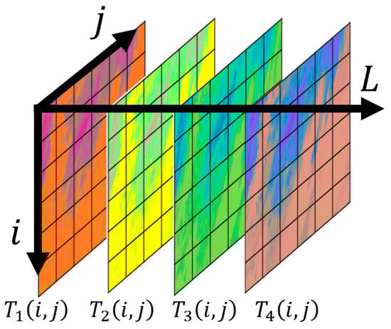
Figure 7.
Four-column data , different colors represent data acquired by different columns of the FPA.
Thus, the uniformity-optimal detector element selection scheme based on the Viterbi algorithm is obtained. To verify the correctness of this algorithm, we conducted a brute-force search on a small-scale dataset to identify the minimum, and the results matched those produced by the Viterbi-based approach, confirming its validity. Using the Viterbi-based selection method, only calculations of IRBTD are required to derive the uniformity-optimal scheme. This significantly reduces computational complexity, making it suitable for real-time onboard operation and enabling BDS for each swath in real time.
2.4. Joint Consideration of Consistency and Sensitivity
In the previous section, we obtained a theoretically consistency-optimal detector selection scheme. While this scheme maximizes image consistency, it does not account for other performance parameters of the detector elements. Traditional detector-selection strategies typically prioritize the individual performance of the detector elements, particularly the sensitivity metric. Therefore, this section will explore a detector-selection strategy that achieves a balance between consistency and sensitivity. It should be noted that in practical applications, the method presented in this paper can also replace sensitivity with other performance metrics or incorporate additional metrics for a comprehensive trade-off.
In the previous section, we treated IRBTD as the “cost” of a selection. When optimizing for uniformity alone, the objective is to minimize the average IRBTD, i.e., to minimize total cost. However, when both uniformity and sensitivity must be considered, the cost cannot be based on IRBTD alone—it must also reflect sensitivity. Therefore, we redefine the cost function to combine IRBTD with a sensitivity term…
where
In (14), denotes the cost associated with selecting a detector element in row i. is the sensitivity-related term defined in (15), where denotes the NEdT of the detector element in column S at row i on the focal plane (in Kelvin). β is a predetermined dimensionless weight coefficient ranging from 0 to 1. A larger β places greater emphasis on uniformity, and when β = 0, the method degenerates to the original approach (i.e., sensitivity-optimal BDS). It should be noted that in Equation (14), IRBTD and NEdT share the same dimension (Kelvin, K), which ensures the validity of their direct linear combination. In this study, no additional normalization was performed; instead, IRBTD (in K) and NEdT (in K) were summed directly via Equation (14). The determination of the weighting coefficient β will be discussed in detail later in the text.
We substitute in (13) with cost(i), thus realizing a BDS scheme that jointly accounts for uniformity and sensitivity. In this formulation, the cost of choosing a detector element in each row depends on both uniformity (via IRBTD(i)) and sensitivity (via ): elements exhibiting better uniformity and higher sensitivity incur a lower cost. Users may also incorporate additional metrics of interest and their corresponding weight coefficients into the cost function. Of course, for evaluation metrics with different dimensions or scales, appropriate non-dimensionalization or normalization is necessary.
The pseudocode is shown in Algorithm 1. The algorithm begins by iterating over every candidate combination of detector elements spanning three consecutive rows, computing the cumulative cost for each via the Viterbi procedure while tracking the minimum cost and its associated choice; once all rows have been processed in this forward pass, a backtracking step is performed to recover the optimal detector element for each row based on the recorded minimum-cost transitions.
| Algorithm 1 Viterbi of BDS |
| Input: [N×K×F], NEdT [N×K], β (0 ≤ β ≤ 1) |
| Output: map [1…N] (selected columns per row) |
cost_dp[1…2,:,:] ← 0.
for k = 1 to K, ℓ = 1 to K (cost_dp[i,k,ℓ], idx[i,k,ℓ]) = argmin_{j = 1 to K} {cost_dp[i − 1,j,k] + c(i,j,k,ℓ)} where c(i,j,k,ℓ) = β · ‖{i − 1,k,:} − ½({i − 2,j,:} + {i,ℓ,:}) ‖1/F + (1 − β)·
map[N − 1] = best_k; map[N] = best_ℓ. for i = N − 2 down to 1 map[i] = idx[i + 2, map[i + 1], map[i + 2]].
|
To verify the linear time complexity and onboard real-time processing capability of the algorithm, this paper analyzes the computational and storage complexity of the proposed Viterbi-based optimizer. The time complexity of the algorithm is , where is the number of focal-plane rows, is the number of detector columns (typically 4 or 6), and is the number of image columns per observation task (for GHI, ). Since both and are sensor-specific constants, the actual computational load of the algorithm grows linearly with . Compared with the exponential complexity of a brute-force enumeration, the proposed method achieves an acceleration of several orders of magnitude. The memory consumption of the algorithm mainly comes from two matrices of size , resulting in a space complexity of and very low storage requirements. Taking FY-4B GHI as an example (), each processing requires only about 1.6 × 10⁷ floating-point operations and several tens of kilobytes of memory. Such a computational load is far below the processing capability of typical space-borne processors (e.g., ARM or LEON running at hundreds of MHz) within an imaging cycle of several seconds, thereby fully demonstrating the feasibility of real-time onboard processing at the algorithmic level.
In contrast, methods based on machine learning or Bayesian optimization may achieve better performance on certain datasets, but they are typically accompanied by higher training costs, greater demands for parameter tuning, and stricter requirements on computational resources and software reliability. These limitations—including the reliance on extensive labeled data, high computational power and power consumption, as well as significant storage demands—are fundamentally at odds with the core constraints of the spaceborne environment, such as limited computing resources, stringent power budgets, tight storage, and the need to withstand radiation risks. Consequently, they are difficult to deploy directly in such scenarios.
In the following chapter, we evaluate the performance of the algorithm, analyze how different values of β affect the BDS results, and propose a recommended strategy for choosing an appropriate β in practical engineering applications.
3. Results
3.1. Preliminary Results
First, we present the remote sensing images reconstructed using the consistency-optimal criterion. Figure 8, Figure 9 and Figure 10 show the imaging results and corresponding IRBTD curves for Sample 1 and Sample 2 under the consistency-optimal BDS map, respectively. Visually, striping noise in the images is markedly suppressed, demonstrating the effectiveness of the proposed method in reducing such noise.
Figure 8.
Image of Sample 1 based on the consistency-optimal BDS: (a) full scene; (b) local enlargement of the red box area.
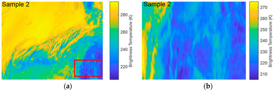
Figure 9.
Image of Sample 2 based on the consistency-optimal BDS: (a) full scene; (b) local enlargement of the red box area.
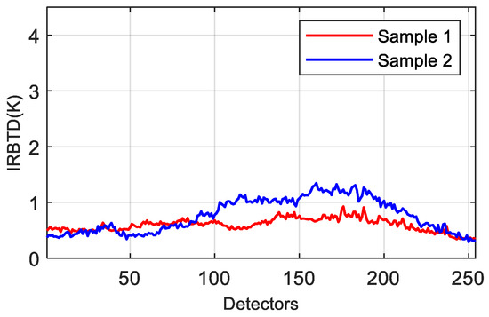
Figure 10.
IRBTD curves of Sample 1 and Sample 2 under the consistency-optimal BDS.
Subsequently, to achieve a balance between consistency and sensitivity, the weighting coefficient β in Equation (13) was initially set to 0.5 and its effect was evaluated. The proposed method was validated using 55 sample datasets from the FY4B-GHI channel 7, which cover diverse observation times, geographic regions and target characteristics. Four representative samples are presented here. Sample 1 focuses on the processing results in low-temperature cloud-top regions; Sample 2 illustrates the scenario with relatively drastic scene variations (where the corresponding IRBTD is generally high); Samples 3 and 4 demonstrate the composite scenario in which the same detector element covers both high-temperature and low-temperature targets simultaneously; additionally, Sample 4 reflects a relatively smooth scene transition (associated with an overall lower IRBTD). The four samples were collected on different days between 25 and 28 June 2022. Each sample represents a 2000 km × 2000 km observational area over a different part of China. This study begins with an in-depth analysis of the four representative samples mentioned above, followed by a report of the aggregated statistics from all samples in Section 3.4. Figure 11, Figure 12, Figure 13, Figure 14, Figure 15, Figure 16, Figure 17 and Figure 18 systematically present the results for these four samples: Figure 11, Figure 13, Figure 15 and Figure 17 compare the remote-sensing images before and after processing for each sample, while Figure 12, Figure 14, Figure 16 and Figure 18 show the corresponding comparisons of IRBTD and NEdT before and after improvement. In these figures, “Baseline” refers to the traditional BDS method, i.e., the sensitivity-optimal (lowest NEdT) BDS strategy, while “Proposed” refers to the BDS method presented in this paper.
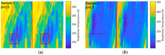
Figure 11.
Comparison of remote sensing images for Sample 1 (baseline method vs. proposed method) with β = 0.5 (the area to the left of the red line shows the baseline method, while the area to the right shows the proposed method): (a) full scene; (b) local enlargement of the red box area.
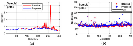
Figure 12.
Comparison of detector-element performance for Sample 1 (baseline method vs. proposed method) with β = 0.5: (a) IRBTD curves; (b) NEdT curves.
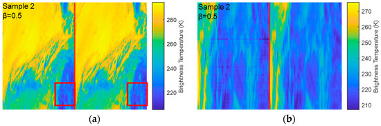
Figure 13.
Comparison of remote sensing images for Sample 2 (baseline method vs. proposed method) with β = 0.5 (the area to the left of the red line shows the baseline method, while the area to the right shows the proposed method): (a) full scene; (b) local enlargement of the red box area.
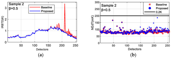
Figure 14.
Comparison of detector-element performance for Sample 2 (baseline method vs. proposed method) with β = 0.5: (a) IRBTD curves; (b) NEdT curves.

Figure 15.
Comparison of remote sensing images for Sample 3 (baseline method vs. proposed method) with β = 0.5 (the area to the left of the red line shows the baseline method, while the area to the right shows the proposed method): (a) full scene; (b) local enlargement of the red box area.
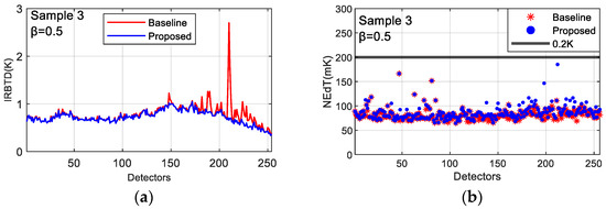
Figure 16.
Comparison of detector-element performance for Sample 3 (baseline method vs. proposed method) with β = 0.5: (a) IRBTD curves; (b) NEdT curves.
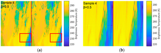
Figure 17.
Comparison of remote sensing images for Sample 4 (baseline method vs. proposed method) with β = 0.5 (the area to the left of the red line shows the baseline method, while the area to the right shows the proposed method): (a) full scene; (b) local enlargement of the red box area.
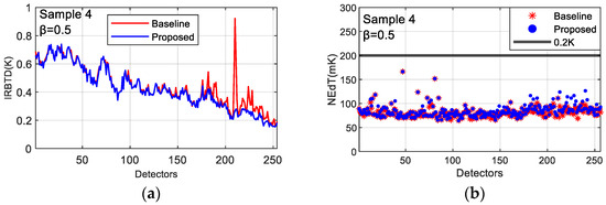
Figure 18.
Comparison of detector-element performance for Sample 4 (baseline method vs. proposed method) with β = 0.5: (a) IRBTD curves; (b) NEdT curves.
It should be noted that the algorithm executes BDS for each swath. For different observation tasks or swaths, the resulting BDS map is essentially the same, which implies that a universal BDS map can be obtained through statistical analysis of a large amount of observational data. Further analysis and study in this regard are beyond the scope of this paper and are therefore omitted.
Visually, the processed remote-sensing images (Figure 11, Figure 13, Figure 15 and Figure 17) exhibit a notable suppression of striping artifacts, presenting a smoother and more homogeneous appearance compared to the raw data. This qualitative improvement is quantitatively corroborated by the corresponding IRBTD line plots (Figure 12, Figure 14, Figure 16 and Figure 18). As illustrated in these plots, the pronounced peaks originally present in the IRBTD curves—which correspond to rows dominated by highly inconsistent detector elements—are substantially attenuated or entirely eliminated after applying the proposed selection algorithm. The plotted lines demonstrate a marked decrease in both the amplitude and variability of row-to-row differences, indicating that the detector-element inconsistencies have been effectively mitigated.
This alignment between visual assessment (Figure 11, Figure 13, Figure 15 and Figure 17) and metric-based analysis (Figure 12, Figure 14, Figure 16 and Figure 18) confirms the efficacy of the method in enhancing image uniformity at the detector-selection stage. Meanwhile, the NEdT result images (embedded in Figure 12, Figure 14, Figure 16 and Figure 18) indicate that the sensitivity loss of the selected detector elements remains at a very low level, which further verifies the effective balance achieved by the weighting coefficient β between consistency improvement and sensitivity preservation.
To quantitatively assess image uniformity, we consider the mean of , denoted . According to (5), we must exclude the contributions of and
From (5) we have:
Similarly, by analogy with IRBTD but swapping “rows” for “columns,” we compute the inter-column brightness temperature difference ICBTD for each sample image (in Kelvin). From prior analysis, ICBTD comprises two components: the intrinsic inter-column variation in the observed target and the variation due to detector noise , as expressed in (17).
Natural scene statistics (NSS) indicate that most natural scenes are approximately spatially stationary and isotropic [32,33]. Consequently, the inter-row variation in the observed target and its inter-column variation are approximately equal, i.e.,
Considering that detector noise is small and approximately stationary and independent, combining (16)–(18) yields:
and therefore
Based on Equation (20), we derive an estimator for the inconsistency parameter , which allows us to preliminarily assess image uniformity—a smaller value indicates better uniformity. It should be noted that the derivations from Equations (16)–(20) hold in a statistical sense for large samples, yet their accuracy for individual specific samples may be limited. Therefore, to more directly quantify the improvement in image uniformity and IRBTD achieved by the proposed method, we calculate for each sample the difference, denoted as ΔIRBTD, between the IRBTD obtained via the conventional sensitivity-optimal selection and that obtained by our method. Subsequently, we adopt the mean and maximum values of ΔIRBTD as evaluation metrics. The relevant results are summarized in Table 2. In the NEdT and columns of Table 2, for each sample, the upper row shows the original BDS results, the lower row (in bold) shows the results produced by the proposed method, and the right column shows the magnitude of change, expressed as the percentage increase in NEdT or the percentage reduction in .
Table 2.
Results of different samples (β = 0.5).
Experimental results indicate that the proposed detector-selection method incurs approximately a 3–7% sensitivity loss compared with a BDS approach targeting sensitivity alone. Meanwhile, striping noise in the images is significantly suppressed, and uniformity improves by 14–40%, indicating a marked enhancement. While NEdT increases by less than 6 mK, the average IRBTD due to inconsistency is reduced by about 20 mK to 0.1 K. For some detectors, the reduction exceeds 3 K. This validates the feasibility and effectiveness of the proposed method in practical applications.
3.2. Discussion of the Weighting Coefficient
The above conclusions refer specifically to the case β = 0.5 in (14). In practice, adjusting β allows a flexible trade-off between sensitivity and uniformity to meet different application requirements. We therefore conducted detector-selection experiments for various β values. Figure 19 illustrates for sample 1 how NEdT and (denoted “NU” in Figure 19) vary with β; both metrics are better when smaller. It can be observed that as β increases from 0 to 1, NEdT rises steadily, whereas first decreases sharply and then more gradually. Analyses of other samples show the same trend. This indicates that for GHI on-orbit data, the β value at the “elbow”—where transitions from a rapid to a more gradual decline—achieves a favorable balance between sensitivity and uniformity, known as the “Elbow Method”.
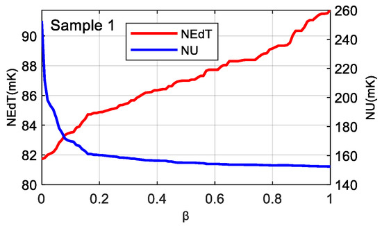
Figure 19.
NEdT and NU vary with β.
Further theoretical analysis indicates that the above method for determining the optimal weighting parameter is not only applicable to GHI but also to other payloads that employ multi-column long linear-array detectors. By plotting NEdT–NU curves for different β (Different β values are shown in different colors in Figure 20), one can clearly observe that the curve bends toward the origin, giving the appearance of being attracted to origin. Selecting the β from this curved region (approximately 0.2 for GHI) yields a good compromise between sensitivity and uniformity. The curve as a whole is very smooth, indicating that a slight variation in the β value does not cause abnormal fluctuations in sensitivity or consistency, demonstrating that the method possesses good stability and broad adaptability. This implies that in practical applications, there is no need to excessively pursue an absolutely precise value of β, which brings considerable convenience to engineering implementation.
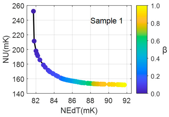
Figure 20.
NEdT–NU for different β.
The shape of this curve can be explained by Pareto-front theory from multi-objective optimization [34,35]: when the two quantities that form the selection criterion (in this case IRBTD and NEdT) are statistically independent and each follows a unimodal (single-peaked) distribution—a condition that holds for almost all payloads—the resulting trade-off curve obtained by the above method will exhibit this characteristic.
Therefore, for different payloads one can follow the same procedure to plot NEdT&NU-β or NEdT-NU curves and thereby determine an appropriate β value. In fact, there is every reason to believe that the proposed method will perform even better for payloads such as ABI, because ABI uses six detector columns while GHI uses only four.
In Table 3, the BDS results for each sample at β = 0.2 are presented. In the NEdT and columns, for each sample, the upper row shows the sensitivity-optimal BDS result, while the lower (bold) row shows the result from the proposed method. At β = 0.2, the remote-sensing images achieve a good balance between sensitivity loss and uniformity improvement. Compared with the sensitivity-optimal BDS, sensitivity loss is reduced to 1–4%—corresponding to an NEdT increase of only about 3 mK—while uniformity improvement remains substantial, with inconsistency decreasing by 10–40%, close to the β = 0.5 case. The corresponding Figure 21, Figure 22, Figure 23, Figure 24, Figure 25, Figure 26, Figure 27 and Figure 28 shows the detailed BDS processing results for β = 0.2.
Table 3.
Results of different samples (β = 0.2).
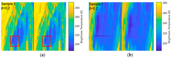
Figure 21.
Comparison of remote sensing images for Sample 1 (baseline method vs. proposed method) with β = 0.2 (the area to the left of the red line shows the baseline method, while the area to the right shows the proposed method): (a) full scene; (b) local enlargement of the red box area.
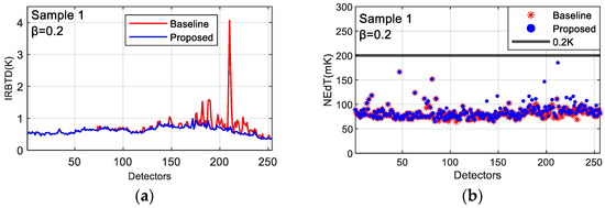
Figure 22.
Comparison of detector-element performance for Sample 1 (baseline method vs. proposed method) with β = 0.2: (a) IRBTD curves; (b) NEdT curves.
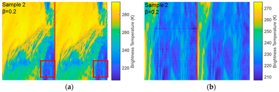
Figure 23.
Comparison of remote sensing images for Sample 2 (baseline method vs. proposed method) with β = 0.2 (the area to the left of the red line shows the baseline method, while the area to the right shows the proposed method): (a) full scene; (b) local enlargement of the red box area.
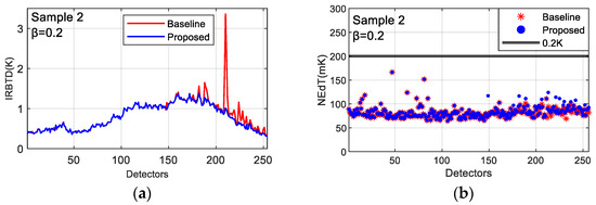
Figure 24.
Comparison of detector-element performance for Sample 2 (baseline method vs. proposed method) with β = 0.2: (a) IRBTD curves; (b) NEdT curves.
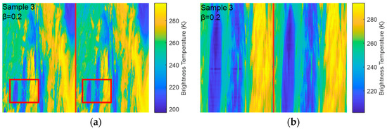
Figure 25.
Comparison of remote sensing images for Sample 3 (baseline method vs. proposed method) with β = 0.2 (the area to the left of the red line shows the baseline method, while the area to the right shows the proposed method): (a) full scene; (b) local enlargement of the red box area.
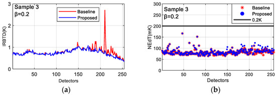
Figure 26.
Comparison of detector-element performance for Sample 3 (baseline method vs. proposed method) with β = 0.2: (a) IRBTD curves; (b) NEdT curves.
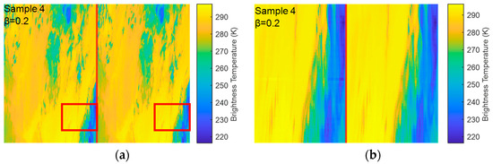
Figure 27.
Comparison of remote sensing images for Sample 4 (baseline method vs. proposed method) with β = 0.2 (the area to the left of the red line shows the baseline method, while the area to the right shows the proposed method): (a) full scene; (b) local enlargement of the red box area.
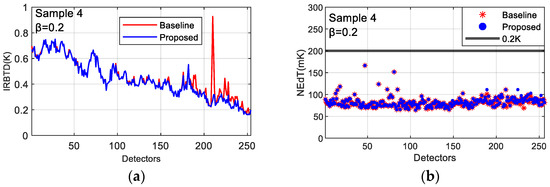
Figure 28.
Comparison of detector-element performance for Sample 4 (baseline method vs. proposed method) with β = 0.2: (a) IRBTD curves; (b) NEdT curves.
3.3. Qualitative and Quantitative Evaluation
Based on the discussion in the previous section, β = 0.2 is identified as a suitable weighting coefficient for GHI. Consequently, in the subsequent evaluation and analysis, we will compare the results obtained with β = 0.2 against those of the baseline method. To comprehensively assess destriping performance, in addition to the IRBTD and NU improvements presented above, we introduce other qualitative and quantitative metrics. Because BDS-based destriping methods almost never discard the true information of original detectors (all candidate detectors represent real measurements), this paper focuses on the suppression of striping noise rather than on evaluating any loss of original information. Specifically, we use the column-direction power spectral density (PSD) for qualitative assessment, and adopt the noise-reduction coefficient (NR) [28,29] and the streaking metric (S) [30] as quantitative evaluation metrics.
Striping noise energy is mainly concentrated in the high-frequency region, particularly near the highest frequency, because the highest frequency corresponds to per-row fluctuation components (i.e., single-row or pixel-scale striping), which are often the most common and pronounced. Figure 29 shows the column PSD curves of samples 1 and 2 before and after processing with the proposed method (β = 0.2). The processed images exhibit a marked reduction in power in the high-frequency band (normalized frequency f > 0.25), and peaks near the highest frequency (normalized frequency f = 0.5) are effectively suppressed. These results indicate that the proposed method can effectively reduce striping components. Experiments on other samples show similar trends, further validating the method’s effectiveness.
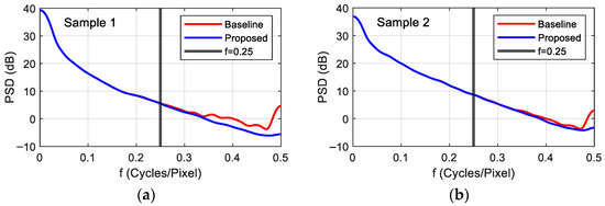
Figure 29.
PSD before and after improvement: (a) Sample1, (b) Sample2.
The NR describes the attenuation of striping noise in the frequency domain and is defined as (21)
where and denote the total power in the striping-noise frequency band before and after processing. NR > 1 indicates a reduction in striping power. In this paper, we compute NR for two frequency bands: (1) the entire high-frequency band f > 0.25 (the high-frequency region mainly affected by striping); and (2) the highest frequency point f = 0.5 (corresponding to single-row striping). The results are shown in Table 4.
Table 4.
Comparison of evaluation metrics.
The results indicate a significant reduction in striping noise power compared to the unprocessed images. Specifically, across the entire high-frequency band affected by striping (normalized frequency f > 0.25), the noise power is reduced by approximately 7% to 45% on average. At the frequency point corresponding to the most representative single-row striping (f = 0.5), the power is further decreased to about 1/2 to 1/10 of the pre-processing level (as reflected in Table 4, where the NR value reaches up to 10.37). This pronounced attenuation in the frequency domain confirms that the proposed method effectively suppresses striping components in the imagery, particularly in the high-spatial-frequency range.
Furthermore, we employ the previously mentioned streaking metric S to evaluate the images in the spatial domain before and after processing. As shown in Table 4, the S values of all samples decrease significantly, with the maximum reduction exceeding 50% (e.g., Sample 1 drops from 0.295% to 0.132%). This result further verifies, from the perspective of spatial distribution, the effectiveness of the proposed method in improving image uniformity and mitigating inter-row inconsistency. Together with the findings from the frequency-domain analysis, these outcomes consistently demonstrate that the introduced detector-selection strategy provides reliable performance for comprehensive striping-noise suppression.
3.4. Overall Performance Evaluation Using All Samples
The previous section provided a detailed analysis of four representative samples. To further validate the robustness and generalization capability of the proposed method under diverse observational conditions, this subsection conducts a statistical evaluation based on a dataset comprising 51 independent sample scanning swaths (File S1 in Supplementary Materials). These samples cover a variety of typical scenarios, including low-temperature regions, high-temperature regions, uniform oceanic or cloud-covered areas, and scenes with strong contrast. Compared to the representative cases presented earlier, this diversified sample set enables a more statistically rigorous verification of the method’s performance.
This section provides an aggregated presentation of three core metrics across all samples: NR, mean ΔIRBTD, and mean ΔNEdT after processing, and analyzes their statistical interrelations. Table 5 presents summary statistics—including the mean, median, standard deviation, and IQR (25th and 75th percentiles)—for ΔIRBTD, ΔNEdT, and two NR metrics (NR (f > 0.25) and NR (f = 0.5)) across the additional 51 independent sample swaths. Since the improvement data for NR and ΔIRBTD exhibit non-normal, long-tailed distributions, we employ the median and interquartile range (IQR), in addition to the mean and standard deviation, to describe their central tendency and dispersion. The analysis reveals:
Table 5.
Statistical Summary of Core Performance Metrics Across 51 Samples.
- (1)
- Uniformity Improvement: The median ΔIRBTD is 31.24 mK, with half of the samples showing improvements concentrated between 20.88 mK and 59.38 mK (IQR). This confirms that the method consistently enhances inter row consistency.
- (2)
- Sensitivity Control: The median ΔNEdT is 2.468 mK (IQR: 1.989–3.480 mK), indicating that the increase in the noise-equivalent temperature difference is strictly limited to a low level, meeting the sensitivity requirements for engineering applications.
- (3)
- Striping-Noise Suppression: The high-frequency noise-reduction coefficient NR (f > 0.25) has a median of 1.082 (IQR: 1.053–1.210). At the highest frequency point (f = 0.5), which represents single-row striping, the median NR reaches 2.953 (IQR: 2.126–5.718), meaning the striping-noise energy at this frequency is reduced on average to approximately 1/3–1/5 of its original level, demonstrating highly significant suppression.
These statistical results confirm that the proposed method delivers consistent and significant performance improvements in the vast majority of samples while maintaining good stability.
To gain deeper insight into the intrinsic relationships among the performance metrics and the method’s adaptability to different scenes, we further plotted the distribution and correlation diagrams of the metrics.
Figure 30 and Figure 31, respectively, show the distribution of the performance metrics across all samples and their inter-relationships. Figure 30 uses ΔIRBTD as the horizontal axis and displays its relationship with NR (f = 0.5) and ΔNEdT. Figure 30 clearly reveals a pronounced positive correlation between ΔIRBTD and NR (f = 0.5): a greater improvement in inter-row brightness-temperature difference corresponds to stronger high-frequency striping suppression. This statistically cross-validates the effectiveness of the proposed method and the rationality of the IRBTD metric. Meanwhile, as NR increases (indicating stronger suppression), ΔNEdT shows a slight upward trend, visually illustrating the inherent engineering trade-off between improved image uniformity and system sensitivity—a design principle fully aligned with the weighted cost function constructed in Section 2.4.
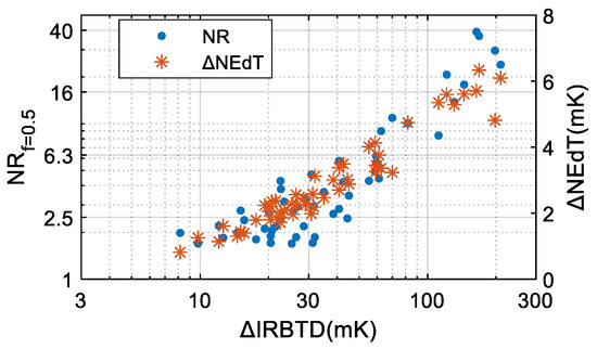
Figure 30.
Correlation Analysis Among ΔIRBTD, NR (f = 0.5), and ΔNEdT.
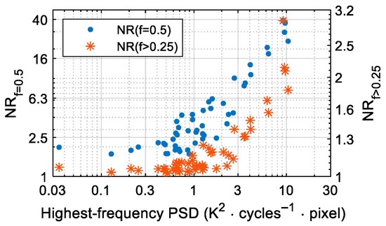
Figure 31.
Relationship Between Highest-Frequency PSD and NR (f > 0.25).
To further evaluate the method’s adaptability and stability under different observational scenarios, we calculated the highest-frequency power spectral density (PSD) for each sample before processing. This metric reflects the intensity of inter-row variation in the image and can serve as a comprehensive indicator of scene complexity and initial striping-noise strength. Figure 31 presents the relationship between the highest-frequency PSD and NR (f > 0.25). The results show that regardless of the initial inter-row variation intensity, all samples achieve consistent improvement (NR > 1) after processing with the proposed method. Moreover, a significant positive correlation exists between the two, indicating that the method delivers more pronounced suppression when the scene inherently contains stronger striping noise or inter-row inconsistency. This further demonstrates that the algorithm retains excellent generalization capability even under diverse operational conditions.
It is worth noting that whether IRBTD- and NU-based metrics are used, or quantitative measures such as NR and S are adopted, the degree of improvement varies significantly across different samples. This variation arises because the severity of inconsistency differs across observation targets and scenes. Several factors may contribute to this phenomenon:
- (1)
- Constrained by Planck’s radiation law, the same signal deviation manifests as stronger inconsistency in low-temperature regions, leading to temperature-dependent differences in uniformity.
- (2)
- The fitting error of a detector element varies with temperature (radiance).
- (3)
- Different targets exhibit distinct spectral emission curves, which, when convolved with the spectral response functions of different detector, result in varying deviations.
- (4)
- The stochastic nature of low-frequency noise.
Therefore, for different observation targets, inconsistency and its potential for improvement should be regarded as spanning a range, rather than as a single fixed value.
4. Discussion
4.1. Limitations
While the proposed method demonstrates good performance in improving image uniformity and achieving sensitivity trade-offs, it is important to acknowledge its limitations. A clear understanding of these boundaries will help readers better assess its applicable scope.
- (1)
- Potential Sensitivity to Extreme Non-uniform Scenes: The core evaluation metric, IRBTD, relies on comparing differences between rows. Although the method shows robustness across the diverse samples validated in this study, in localized areas with extremely intense inter-row radiance variation, the intrinsic scene signal may dominate the IRBTD calculation. This could potentially lead the algorithm to select detectors that appear relatively consistent locally but may not possess the optimal absolute radiometric accuracy. This phenomenon and its practical impact will be further examined in future work using larger datasets.
- (2)
- Performance Bound Constrained by Raw Data Quality: The method essentially performs optimal combination of detector data without altering the original measurements. Consequently, the theoretical upper bound for striping suppression is determined by the best inherent consistency present in the raw data. If all candidate detectors for a given row exhibit significant and similar response deviations, the method cannot surpass this physical limitation to fundamentally generate superior consistency.
- (3)
- Generalizability and Adaptive Challenge of Parameter β: Although this study proposes a practical strategy based on the “Elbow Method” for determining the trade-off coefficient β using substantial data, its optimal value may fluctuate with the evolving on-orbit status of the instrument. Furthermore, the best β value might vary subtly for different types of observation targets. Future work will explore the possibility of adaptive determination of β based on real-time scene content to enhance the intelligence and applicability of the method.
- (4)
- Validation Scope Limited by Sensor Characteristics: It should be noted that due to the radiometric characteristics of the long-wave infrared band and the kilometer-scale spatial resolution used in this study, each individual pixel receives a blended signal of thermal radiation from a large surface area. Consequently, fine-scale man-made structures cannot be effectively resolved, and dedicated validation for such scenes is not feasible. Nevertheless, validation has been conducted across a variety of typical natural scenarios, and the results adequately demonstrate that the proposed method possesses broad applicability for infrared-band observations from geostationary meteorological satellites, which is its primary design objective.
These limitations also highlight that the proposed method complements rather than replaces existing image-based destriping techniques. The detector-selection framework ensures physical authenticity and radiometric consistency at the data source, providing a reliable foundation for downstream quantitative applications. Image post-processing algorithms, on the other hand, can perform fine-grained adjustments at the pixel level to further suppress residual stripes. An integrated approach—combining source optimization with pixel refinement—holds promise for achieving superior overall image quality and represents an important and promising direction for future research.
Acknowledging these limitations, and building upon the method’s demonstrated stability and linear computational efficiency, we proceed to propose the following engineering deployment recommendations to facilitate its practical adoption.
4.2. Engineering Implementation Recommendations
For the practical implementation and deployment of the proposed method in engineering applications, we provide the following recommendations.
During the on-orbit testing phase, a diverse scene dataset covering the sensor’s full dynamic range and containing multiple typical target types should be systematically collected, and an appropriate β value should be determined based on this dataset. In the initial phase of operational running, the parameter can be fine-tuned slightly according to feedback from actual image products. Since minor changes in the β value do not lead to significant fluctuations in algorithm performance, even if the optimal β varies slightly for different targets, its impact on the final results is quite limited. In practical engineering, a β value that performs stably and acceptably across all typical scene types can be selected. By plotting NEdT–NU curve clusters for various scenes, a β value with good generalization capability can be chosen. Although this value may not be the optimum for any single scene, it can ensure an overall superior and predictable performance trade-off throughout the entire mission lifecycle.
Once β is determined, two deployment strategies may be considered:
- (1)
- Real-time strip-wise BDS (recommended for scenarios with the highest performance requirements):
For each swath, the BDS map is calculated and applied in real time. This strategy ensures that every observation achieves the optimal balance, thereby maximizing the suppression of bad lines and striping noise. However, frequent updates of the BDS map may impose greater demands on computational resources, system stability, and software reliability, thus increasing implementation and maintenance costs.
- (2)
- Pre-computed and fixed BDS maps derived from statistically representative data (recommended for scenarios prioritizing operational stability):
In this strategy, a large volume of representative on-orbit data is used offline to statistically derive several general-purpose BDS maps, which are then fixed for use during routine operations. This approach is simple, stable in operation, and convenient for engineering deployment and long-term maintenance. However, its performance is usually somewhat inferior to real-time strip-wise updating.
The deployment strategies above aim to achieve an optimal balance based on current data and understanding. To further extend the boundaries of this method and verify its long-term consistency and generalizability, we outline the following directions for future research.
4.3. Future Prospects
In the authors’ current dataset, the BDS maps derived from different scanning strips exhibit good consistency. To further verify this consistency and to assess the general applicability of the method, future work will include:
- (1)
- Further explore an adaptive mechanism that dynamically adjusts the β value based on real-time scene classification—for example, by utilizing synchronously observed visible channels or the intrinsic statistical characteristics of the data—thereby advancing the method toward an intelligent and scene-aware direction.
- (2)
- Collecting and analyzing a larger volume of on-orbit data to evaluate the consistency of BDS maps under different observation conditions, and to investigate whether a general-purpose BDS map suitable for long-term operations exists.
- (3)
- Reproducing and validating the applicability of the proposed method using data from different payloads.
- (4)
- Verifying whether the improved data deliver better performance in downstream applications.
5. Conclusions
This study proposes a fundamentally different approach to address striping noise. Unlike conventional calibration optimization or image post-processing, for next-generation geostationary satellite imagers equipped with multi-column long-linear-array detectors, our method is the first to systematically start from the source—detector selection—directly suppressing striping noise during the image synthesis stage. This ensures that all output pixels originate from genuine physical measurements, thereby completely avoiding the information loss and artificial distortion commonly associated with image post-processing.
The innovativeness of the method is reflected in several closely linked aspects: First, an on-board-suitable metric for detector inconsistency—the Inter-row Brightness Temperature Difference (IRBTD)—is proposed, providing a reliable basis for real-time evaluation and selection in orbit. Second, the Viterbi algorithm is introduced for the first time into the detector-element selection problem, transforming the global optimization task into a dynamic-programming solution with linear complexity. This enables efficient, globally optimal searching within a vast combinatorial space, meeting the stringent computational efficiency requirements for real-time on-board processing. Furthermore, by designing a weighted cost function that integrates IRBTD and NEdT, an effective and flexible trade-off between striping-noise suppression and system sensitivity is achieved for the first time within a detector-selection framework, along with a practical strategy for determining the weighting coefficient in engineering applications. Finally, these elements together constitute a systematic and complete solution for suppressing striping noise from the selection perspective.
Experiments on FY-4B GHI data fully validate the effectiveness of the framework. The results show that image uniformity is significantly improved with minimal sensitivity loss: NEdT increases by only 1–4% (absolute increase ≤ 4 mK), while inconsistency is reduced by 10–40%, the average IRBTD decreases by approximately 20–100 mK, and improvements for some detector elements exceed 3 K. Multi-metric evaluation in both the frequency and spatial domains further confirms notable striping-noise suppression: power spectral density analysis indicates that the high-frequency band energy is reduced by about 7–45%, and the power at the highest frequency point, corresponding to single-row striping, drops to 1/2–1/10 of the original level; the streaking metric S decreases by an average of about 50%, with a maximum reduction exceeding 55%.
In summary, this work not only demonstrates the feasibility of suppressing striping noise at the source through optimized detector selection, but also provides a complete solution that combines theoretical rigor, engineering practicality, and data fidelity. The framework requires no modification of the calibration process nor the introduction of image-restoration algorithms, preserving the authenticity of the observational data. It offers a reliable and general enhancement approach for improving the data quality of scanning radiometers that employ multi-column redundant architectures.
Supplementary Materials
The following supporting information can be downloaded at: https://www.mdpi.com/article/10.3390/rs18020233/s1, File S1: Detailed Data and Analysis Results for All Samples in Section 3.4.
Author Contributions
Conceptualization, X.J.; methodology, X.J., T.W. and X.L.; software, X.J., T.W. and X.L.; validation, X.J. and T.W.; formal analysis, X.J.; investigation, X.J. and X.L.; resources, X.L. and C.H.; data curation, X.L. and C.H.; writing—original draft preparation, X.J.; writing—review and editing, X.J., X.L. and C.H.; visualization, X.J.; supervision, X.L. and C.H.; project administration, C.H.; funding acquisition, X.L. and C.H. All authors have read and agreed to the published version of the manuscript.
Funding
This research was funded by State Key Program of National Natural Science Foundation of China (Grant No. 42330110).
Data Availability Statement
The data supporting the findings of this study are available from the corresponding author upon reasonable request.
Conflicts of Interest
The authors declare no conflicts of interest.
Abbreviations
The following abbreviations are used in this manuscript:
| NEdT | Noise-Equivalent Temperature Difference |
| IRBTD | Inter-Row Brightness Temperature Difference |
| GHI | Geostationary High-speed Imager |
| BDS | Best Detector-element Selection |
| ABI | Advanced Baseline Imager |
| AHI | Advanced Himawari Imager |
| AMI | Advanced Meteorological Imager |
| FCI | Flexible Combined Imager |
| FY-4B | FengYun-4B |
| GOES | Geostationary Operational Environmental Satellite |
| GEO-KOMPSAT | Geostationary Korea Multi-Purpose Satellite |
| MTG | Meteosat Third Generation |
| ICBTD | Inter-Column Brightness Temperature Difference |
| PSD | Power Spectral Density |
| NR | Noise-Reduction coefficient |
| EM | Example Matrix |
| FPA | Focal Plane Array |
| IFOV | Instantaneous Field Of View |
| SNR | Signal-to-Noise Ratio |
| NSS | Natural Scene Statistics |
References
- Li, B.; Zhou, Y.; Xie, D.; Zheng, L.; Wu, Y.; Yue, J.; Jiang, S. Stripe Noise Detection of High-Resolution Remote Sensing Images Using Deep Learning Method. Remote Sens. 2022, 14, 873. [Google Scholar] [CrossRef]
- Qian, H.; Wu, X.; Yu, F.; Shao, S.; Iacovazzi, R.; Wang, Z.; Hyelim, H. Detection and characterization of striping in GOES-16 ABI VNIR/IR bands. In Proceedings of the SPIE Earth Observing Systems XXIII, San Diego, CA, USA, 19–23 August 2018; Volume 10764, p. 107641N. [Google Scholar] [CrossRef]
- Di, D.; Liu, Y.; Li, J.; Zhou, R.; Li, Z.; Gong, X. Inter-calibration of geostationary imager infrared bands using a hyperspectral sounder on the same platform. Geophys. Res. Lett. 2023, 50, e2022GL101628. [Google Scholar] [CrossRef]
- Efremova, B.; Pearlman, A.J.; Padula, F.; Wu, X. Detector level ABI spectral response function: FM4 analysis and comparison for different ABI modules. In Proceedings of the SPIE Earth Observing Systems XXI, San Diego, CA, USA, 28 August–1 September 2016; Volume 9972. [Google Scholar] [CrossRef]
- Padula, F.; Cao, C. Detector-level spectral characterization of the Suomi NPP Visible Infrared Imaging Radiometer Suite long-wave infrared bands M15 and M16. Appl. Opt. 2015, 54, 5109–5116. [Google Scholar] [CrossRef]
- Pearlman, A.J.; Padula, F.; Cao, C. The GOES-R Advanced Baseline Imager: Detector spectral response effects on thermal emissive band calibration. In Proceedings of the SPIE Sensors, Systems, and Next-Generation Satellites XIX, Toulouse, France, 21–24 September 2015; Volume 9639, p. 96390J. [Google Scholar] [CrossRef]
- Chen, W.; Li, B. Overcoming Periodic Stripe Noise in Infrared Linear Array Images: The Fourier-Assisted Correlative Denoising Method. Sensors 2023, 23, 8716. [Google Scholar] [CrossRef]
- Jia, X.; Li, X.; Wang, Z.; Han, C. Detection and Correction of Crosstalk Within Channels of Long-Linear-Array Detectors. IEEE Trans. Geosci. Remote Sens. 2025, 63, 5000616. [Google Scholar] [CrossRef]
- Zhang, M.; Carder, K.; Müller-Karger, F.E.; Lee, Z.; Goldgof, D.B. Noise Reduction and Atmospheric Correction for Coastal Applications of Landsat Thematic Mapper Imagery. Remote Sens. Environ. 1999, 70, 167–180. [Google Scholar] [CrossRef]
- Huang, L.; Gao, M.; Yuan, H.; Li, M.; Nie, T. Stripe Noise Removal Algorithm for Infrared Remote Sensing Images Based on Adaptive Weighted Variable Order Model. Remote Sens. 2024, 16, 3189. [Google Scholar] [CrossRef]
- Ando, K.; Hosoda, K.; Murakami, H. A bispectral approach for destriping and denoising the sea surface temperature product of GCOM-C1/SGLI. J. Atmos. Ocean. Technol. 2023, 40, 181–196. [Google Scholar] [CrossRef]
- Li, Y.; Zhang, H.; Xue, X.; Jiang, Y.; Shen, H. Estimation of sea surface temperature in the Arctic based on microwave radiometer data. J. Mar. Sci. Appl. 2025, 3, 11. [Google Scholar] [CrossRef]
- Wang, Z.; Wu, X.; Yu, F.; Fulbright, J.P.; Kline, E.; Yoo, H.; Schmit, T.J.; Gunshor, M.M.; Coakley, M.; Black, M.; et al. On-orbit calibration and characterization of GOES-17 ABI IR bands under dynamic thermal condition. J. Appl. Remote Sens. 2020, 14, 034527. [Google Scholar] [CrossRef]
- Gunshor, M.M.; Schmit, T.J.; Pogorzala, D.; Lindstrom, S.; Nelson, J.P. GOES-R series ABI imagery artifacts. J. Appl. Remote Sens. 2020, 14, 032411. [Google Scholar] [CrossRef]
- Yu, F.; Wu, X.; Yoo, H.; Qian, H.; Shao, X.; Wang, Z. Radiometric calibration accuracy and stability of GOES-16 ABI infrared radiance. J. Appl. Remote Sens. 2021, 15, 048504. [Google Scholar] [CrossRef]
- Datla, R.; Shao, X.; Cao, C.; Wu, X. Comparison of the calibration algorithms and SI traceability of MODIS, VIIRS, GOES, and GOES-R ABI sensors. Remote Sens. 2016, 8, 126. [Google Scholar] [CrossRef]
- Hu, Y.; Gu, R.; Yu, H.; Li, X.-M.; Dou, C.; Jia, G.; Si, Y.; Zhang, L. Evaluation of the Radiometric Calibration of FY-4A-AGRI Thermal Infrared Data Using Lake Qinghai. IEEE Trans. Geosci. Remote Sens. 2021, 59, 8040–8050. [Google Scholar] [CrossRef]
- Sun, L.; Neville, R.A.; Staenz, K.; White, H.P. Automatic destriping of Hyperion imagery based on spectral moment matching. Can. J. Remote Sens. 2008, 34, S68–S81. [Google Scholar] [CrossRef]
- Wang, E.; Jiang, P.; Li, X.; Cao, H. Infrared stripe correction algorithm based on wavelet decomposition and total variation-guided filtering. J. Eur. Opt. Soc. Rapid Publ. 2019, 16, 1. [Google Scholar] [CrossRef]
- Yan, F.; Wu, S.; Zhang, Q.; Liu, Y.; Sun, H. Destriping of Remote Sensing Images by an Optimized Variational Model. Sensors 2023, 23, 7529. [Google Scholar] [CrossRef]
- Chang, Y.; Chen, M.; Yan, L.; Zhao, X.-L.; Li, Y.; Zhong, S. Toward Universal Stripe Removal via Wavelet-Based Deep Convolutional Neural Network. IEEE Trans. Geosci. Remote Sens. 2020, 58, 2880–2897. [Google Scholar] [CrossRef]
- Kalluri, S.; Alcala, C.; Carr, J.; Griffith, P.; Lebair, W.; Lindsey, D.T.; Race, R.; Wu, X.; Zierk, S. From photons to pixels: Processing data from the advanced baseline imager. Remote Sens. 2018, 10, 177. [Google Scholar] [CrossRef]
- Zhu, Z.; Gu, J.; Xu, B.; Shi, C. Characterization of Himawari-8/AHI to Himawari-9/AHI infrared observations continuity. Int. J. Remote Sens. 2023, 45, 121–142. [Google Scholar] [CrossRef]
- Zhang, B.; Ichii, K.; Li, W.; Yamamoto, Y.; Yang, W.; Sharma, R.C.; Yoshioka, H.; Obata, K.; Matsuoka, M.; Miura, T. Evaluation of Himawari-8/AHI land surface reflectance at mid-latitudes using LEO sensors with off-nadir observation. Remote Sens. Environ. 2025, 316, 114491. [Google Scholar] [CrossRef]
- Kim, D.; Gu, M.; Oh, T.-H.; Kim, E.-K.; Yang, H.-J. Introduction of the Advanced Meteorological Imager of Geo-Kompsat-2a: In-Orbit Tests and Performance Validation. Remote Sens. 2021, 13, 1303. [Google Scholar] [CrossRef]
- Mousivand, A.; Straif, C.; Burini, A.; Lekouara, M.; Debaecker, V.; Hewison, T.; Stock, S.; Bojkov, B. In-Flight Calibration of Geostationary Meteorological Imagers Using Alternative Methods: MTG-I1 FCI Case Study. Remote Sens. 2025, 17, 2369. [Google Scholar] [CrossRef]
- NOAA Cooperative Working Group. SOP for ABI Image Striping (Version 0.4). NOAA STAR. 29 April 2020. Available online: https://www.star.nesdis.noaa.gov/GOESCal/docs/pdf/SOP/CWG-2020-04-29_SOP-for-ABI-Image-Striping_v0.4.pdf (accessed on 3 December 2025).
- Shen, H.; Zhang, L. A MAP-Based Algorithm for Destriping and Inpainting of Remotely Sensed Images. IEEE Trans. Geosci. Remote Sens. 2009, 47, 1492–1502. [Google Scholar] [CrossRef]
- Wang, J.-L.; Huang, T.-Z.; Ma, T.-H.; Zhao, X.-L.; Chen, Y. A sheared low-rank model for oblique stripe removal. Appl. Math. Comput. 2019, 360, 167–180. [Google Scholar] [CrossRef]
- Cook, M.; Padula, F.; Pogorzala, D.; Pearlman, A.J.; McCorkel, J.; Krimchansky, A. Reflective solar band striping mitigation method for the GOES-R series advanced baseline imager using special scans. J. Appl. Remote Sens. 2020, 14, 032409. [Google Scholar] [CrossRef]
- Shlezinger, N.; Farsad, N.; Eldar, Y.C.; Goldsmith, A.J. ViterbiNet: A deep learning-based Viterbi algorithm for symbol detection. IEEE Trans. Wirel. Commun. 2020, 19, 3319–3331. [Google Scholar] [CrossRef]
- Ruderman, D.L. The statistics of natural images. Netw. Comput. Neural Syst. 1994, 5, 517–548. [Google Scholar] [CrossRef]
- Mittal, A.; Moorthy, A.K.; Bovik, A.C. No-Reference Image Quality Assessment in the Spatial Domain. IEEE Trans. Image Process. 2012, 21, 4695–4708. [Google Scholar] [CrossRef]
- Emmerich, M.T.M.; Deutz, A.H. A tutorial on Mult-objective optimization: Fundamentals and evolutionary methods. Nat. Comput. 2018, 17, 585–609. [Google Scholar] [CrossRef]
- Petchrompo, S.; Coit, D.W.; Brintrup, A.; Wannakrairot, A.; Parlikad, A.K. A review of Pareto pruning methods for multi-objective optimization. Comput. Ind. Eng. 2022, 167, 1080f22. [Google Scholar] [CrossRef]


Disclaimer/Publisher’s Note: The statements, opinions and data contained in all publications are solely those of the individual author(s) and contributor(s) and not of MDPI and/or the editor(s). MDPI and/or the editor(s) disclaim responsibility for any injury to people or property resulting from any ideas, methods, instructions or products referred to in the content. |
© 2026 by the authors. Licensee MDPI, Basel, Switzerland. This article is an open access article distributed under the terms and conditions of the Creative Commons Attribution (CC BY) license.