Generation of Rainfall Maps from GK2A Satellite Images Using Deep Learning

Highlights

What are the main findings?

• The proposed deep-learning framework—guided by a Pix2Pix-based architecture to generate correlation-informed rainfall fields—produces high-resolution (2 km/10-min) rainfall maps using only GK2A satellite imagery, surpassing previous approaches in spatiotemporal detail.
• The ensemble model (Model-ENS), integrating Model-HSP and Model-CMX, significantly improves estimation accuracy, achieving a year-long correlation nearly four times higher than the operational GK2A QPE.

What are the implications of the main findings?

• The proposed framework demonstrates that accurate precipitation estimation is feasible even in radar-sparse or radar-limited regions by relying solely on geostationary satellite imagery.
• It enables near real-time, high-resolution rainfall monitoring and can be adapted to other geostationary satellite platforms, offering broad applicability for global climate analysis and disaster risk reduction.

Abstract

Accurate rainfall monitoring is essential for mitigating hydrometeorological disasters and understanding hydrological changes under climate change. This study presents a deep learning-based rainfall estimation framework using multispectral GEO-KOMPSAT-2A (GK2A) satellite imagery. The analysis primarily focuses on daytime observations to take advantage of visible channel information, which provides richer representations of cloud characteristics during daylight conditions. The core model, Model-HSP, is built on the Pix2PixCC architecture and trained with Hybrid Surface Precipitation (HSP) data from weather radar. To further enhance accuracy, an ensemble model (Model-ENS) integrates the outputs of Model-HSP and a radar based Model-CMX, leveraging their complementary strengths for improved generalization, robustness, and stability across rainfall regimes. Performance was evaluated over two periods—a one year period from May 2023 to April 2024 and the August 2023 monsoon season—at 2 km and 4 km spatial resolutions, using RMSE and CC as quantitative metrics. Case analyses confirmed the superior capability of Model-ENS in capturing rainfall distribution, intensity, and temporal evolution across diverse weather conditions. These findings show that deep learning greatly enhances GEO satellite rainfall estimation, enabling real-time, high-resolution monitoring even in radar sparse or limited coverage regions, and offering strong potential for global and regional hydrometeorological and climate research applications.

1. Introduction

Accurate rainfall measurement is essential for effective management of water resources and mitigating the impact of natural disasters [1]. Climate change has recently increased the frequency and intensity of extreme weather events, such as heavy rain, floods, and typhoons, making precise rainfall estimation increasingly important. Traditionally, rainfall has been estimated using various measurement tools, including rain gauges, weather radars, and satellites. Rain gauges are critical instruments as they provide the only direct and accurate measurements of surface rainfall. Rain gauges are usually used as the primary reference for validating and calibrating remote sensing tools such as weather radars [2,3,4]. However, rain gauges provide point-based measurements, which, although accurate, offer limited spatial coverage and cannot represent the full extent of a precipitation system. They also require physical installation at each location, restricting observations to instrumented sites.

In contrast, weather radars observe precipitation in much wider areas than rain gauges and provide valuable information on the spatial structure and evolution of rainfall systems [5]. In addition, weather radar measurements provide accurate precipitation in real time and play a key role in the forecast of flash floods and extreme rainfall [6]. However, estimating rainfall using weather radar has several limitations. First, radar coverage is limited because, similar to rain gauges, radars require physical installation and cannot be deployed in regions with complex orography or along coasts [7]. Second, weather radars can detect not only precipitation but also non-precipitation signals such as birds, chaff, and anomalous propagation, leading to errors in rainfall estimation [8,9].

In addition to ground-based instruments, meteorological agencies worldwide have, since the 2010s, launched and operated advanced geostationary satellites equipped with multi-spectral imagers of comparable specifications to enhance atmospheric observation, monitoring, and forecasting capabilities. These satellites have become key assets in expanding global capacity for continuous and comprehensive meteorological observations. The Advanced Baseline Imager (ABI) aboard NOAA’s Geostationary Operational Environmental Satellite (GOES)-R series, launched in 2016, provides 16 spectral bands designed for comprehensive analysis of atmospheric conditions [10]. The Flexible Combined Imager (FCI) aboard EUMETSAT’s Meteosat Third Generation (MTG), launched in 2022, also features 16 spectral bands that improve the detection of thin cirrus clouds, aerosols, and localized fire events [11]. The Advanced Geosynchronous Radiation Imager (AGRI) aboard China’s Fengyun-4 (FY-4) satellite, launched in 2016, includes 14 spectral bands for monitoring rapidly evolving weather systems and enhancing early warning and forecasting capabilities [12]. The Advanced Himawari Imager (AHI) aboard Himawari-8/9, Japan’s new generation of geostationary meteorological satellites launched in 2015, provides 16 spectral bands and shortened revisit times compared to the Multifunctional Transport Satellite (MTSAT-2), enabling improved identification and tracking of rapidly changing weather phenomena [13].

The Korea Meteorological Administration (KMA) also operates geostationary weather satellites. The GEO-KOMPSAT-2A (Geostationary Korean Multi-Purpose Satellite 2A, GK2A), launched in 2018, is a new generation of Korean geostationary meteorological satellites. It carries state-of-the-art optical sensors with significantly higher radiometric, spectral, and spatial resolution than the previously available Communication, Ocean, and Meteorological Satellite (COMS) in geostationary orbit. The new Advanced Meteorological Imager (AMI) on the GK2A has 16 observation channels, providing a spatial resolution of 0.5 to 2 km and a temporal resolution of 2 to 10 min. These capabilities offer significant improvements in nowcasting services and short-range weather forecasting systems [14].

All these geostationary satellites provide a broad view of clouds systems and global weather phenomena, as they remain consistently positioned in geostationary orbit. Furthermore, their high spatial and temporal resolutions make them highly effective tools for meteorological observations.

In addition to geostationary satellites, low Earth orbit (LEO) satellites also provide rainfall measurements through microwave observations. The Tropical Rainfall Measuring Mission (TRMM), launched by NASA and JAXA in 1997, provided important precipitation information using several space-borne instruments to enhance our understanding of the interactions between water vapor (WV), clouds, and precipitation [15]. Following the success of TRMM, the Global Precipitation Measurement (GPM) Core observatory satellite was launched in 2014, carrying advanced radar and radiometer systems to improve the accuracy and consistency of precipitation measurements. The GPM Core observatory satellite is equipped with the Dual-frequency Precipitation Radar (DPR) and GPM Microwave Imager (GMI) to provide reference data for global precipitation [16].

Satellite-based precipitation estimation methods typically rely on information from the visible/infrared (VIS/IR) channels, passive microwave (PMW), and active microwave (AMW). VIS/IR observations from GEO satellites focus on the relationship between cloud-top temperature and rainfall intensity at the ground. It is important to note that these methods provide indirect estimates of rainfall [17,18]. However, PMW and AMW sensors, which are deployed on LEO satellites, provide the most direct measurements of precipitation but suffer from poor temporal and lower spatial resolutions compared to GEO satellites, as their long revisit times often span several days [19,20]. Nonetheless, AMW sensors can capture detailed three-dimensional information, allowing for a better understanding of precipitation systems [21]. Although geostationary (GEO) observation systems are known to have lower accuracy compared to passive microwave (PMW) sensors on low Earth orbit (LEO) satellites, they remain highly valuable for hydrological applications and rainfall monitoring. In particular, GEO sensors provide continuous coverage over broad regions with high temporal resolution, enabling near real-time detection of rapidly evolving precipitation and convective activity. Their low latency is also advantageous for weather forecasting, disaster response, and flood early warning systems, where timely information is critical. These characteristics underscore the importance of GEO observations as a research focus, as GEO data posess substantial practical utility for precipitation extimation and hydrological operations even if their sensor level accuracy does not match that of LEO PMW systems. By combining data from VIS/IR observations, PMW sensors, and AMW sensors, a variety of advanced satellite-based precipitation estimation products have been developed over the past two decades. Representative examples include the Enterprise Rain Rate (ERR), which is the latest NOAA Enterprise implementation that replaces the previous GOES-R Rainfall Rate/SCaMPR operational algorithm while remaining grounded in the SCaMPR [22] family of IR–MW blended retrieval concepts; the JAXA Global Satellite Mapping of Precipitation (GSMaP) [23,24]; the NOAA CPC Morphing Technique (CMORPH) [25]; and the NASA Integrated Multi-satellitE Retrievals for GPM (IMERG) [26,27].

Recent advancements in artificial intelligence have reached a significant level and are widely applied across various fields. Many studies have attempted to combine deep learning techniques with satellite imagery to enhance rainfall estimation. As one of the early studies applying artificial intelligence to precipitation estimation, Chen et al. [28] developed a multi-layer perceptron (MLP) model trained on a combined dataset of geostationary satellite observations and dual-polarization ground radar measurements, demonstrating the potential of AI-based data fusion for improving rainfall retrieval accuracy. The PERSIANN-CNN model [29] represents another early application of artificial intelligence to satellite-based precipitation estimation, leveraging convolutional neural networks (CNNs) with IR and WV channels from geostationary satellites. As one of the pioneering studies in this domain, it demonstrated significantly improved rainfall detection performance over traditional models, highlighting the potential of deep learning for remote sensing applications. The PERSIANN-CNN model outperformed baseline algorithms such as PERSIANN-CCS and PERSIANN-SDAE in terms of both the Critical Success Index (CSI) and Root Mean Square Error (RMSE). Similarly, Moraux et al. [30] developed a model that estimates rainfall using geostationary satellite observations and automatic rain gauge measurements by leveraging a CNN-based semantic segmentation approach, demonstrating its ability to effectively capture convective precipitation patches. Extending beyond standard CNN frameworks, U-Net-based architectures have also been adopted to integrate geographical and IR information for more accurate satellite-based precipitation retrieval. Applying an appropriate U-Net-based CNN architecture has been shown to significantly enhance the accuracy of satellite-derived precipitation products [31].

Beyond the use of basic CNN architectures, subsequent studies have explored more advanced generative and segmentation-based models for precipitation estimation. Hayatbini et al. [32] proposed a network trained using the non-saturating conditional Generative Adversarial Network (cGAN) and Mean Squared Error (MSE) loss terms to generate results that better capture the complex distribution of precipitation in the observed data. The results showed improvements in precipitation retrieval accuracy in the proposed framework compared to baseline models trained using conventional MSE loss terms. Berthomier et al. [33] presented the Espresso model to estimate precipitation using satellite data from the Global Precipitation Measurement Core Observatory. They used DeepLabv3+, which has been widely employed for image segmentation tasks. The model demonstrated the ability to detect and accurately estimate rainfall. Ma et al. [34] proposed a Multi-SpatioTemporal network (DLPE-MST) which integrates 3D convolutional neural networks (3D CNNs) to capture motion features from GOES-16 multitemporal bispectral images (6.19 and 10.35 µm) for near-real-time rainfall estimation. This model efficiently generates high-resolution rainfall maps in just 0.09 s per raster, highlighting its potential for real-time operational precipitation monitoring. Liu et al. [35] proposed a novel precipitation estimation method based on FY-4B meteorological satellite data (FY-4B_AI). An evaluation of over 450 million station cases in 2023 showed that FY-4B_AI generally outperforms GPM/IMERG-L in multiple metrics, while showing comparable performance in representing strong weather events across different climatic regions. Dao et al. [36] evaluated the PERSIANN-Dynamic Infrared Rain Rate near real-time product (PDIR-Now) in the Western U.S. and examined bias correction using U-Net, Efficient-UNet, and cGAN models. By incorporating digital elevation data, these models better captured complex orographic precipitation patterns. The results showed that Efficient-UNet and cGAN outperformed both PDIR-Now and U-Net across multiple metrics, highlighting their potential for improved water resource management.

A summary of recent AI-based studies on satellite-based precipitation estimation is provided in Table 1 for reference. Unlike previous approaches that primarily relied on reflectivity-based training (e.g., PERSIANN-CNN, U-Net, DeepLabv3+), our framework directly learns HSP features for end-to-end precipitation estimation and incorporates the Inspector module from Pix2PixCC to guide the learning process, resulting in improved statistical consistency and the preservation of meaningful correlation structures in the estimated rainfall fields.

Table 1. Summary of recent AI-based precipitation estimation studies. Note: Bold indicates the model proposed and used in this study.

Reference/Study	Model	Resolution	Coverage	Source
Moraux et al., 2019 [30]	CNN	3 km/15 min	Belgium	GEO, Gauge
Hayatbini et al., 2019 [32]	cGAN	4 km/30 min	United States	GEO, Radar
Sadeghi et al., 2020 [31]	U-Net	4 km/1 h	United States	GEO, LEO_rain
Berthomier and Perier, 2023 [33]	DeepLabv3+	5 km/30 min	Global	GEO, LEO_rain
Ma et al., 2024 [34]	DLPE-MST	4°/1 h	Continental United States	GEO, Radar
Liu et al., 2024 [35]	LGBM	0.5–4 km/5–7 min	China	Radar, GPM, Rain Gauge
Dao et al., 2025 [36]	UNet, Efficient-UNet, cGAN	4 km/3 h	Western U.S.	PDIR-Now, DEM
Ours	Pix2PixCC	2 km/10 min	Korea	GEO, Radar

Building on this framework, this study employs the Pix2PixCC-based architecture to enhance precipitation estimation. The Pix2PixCC model was originally proposed by Jeong et al. [37] as an improved version of Pix2PixHD [38], which was designed for high-resolution image-to-image translation. In Pix2PixCC, an inspector network was incorporated to guide the generator in producing outputs that are physically consistent with the input data. Building on this framework, Yim [39] (hereafter referred to as Model-CMX) developed a model to generate weather radar maps from GK2A satellite images over South Korea. Model-CMX was trained to predict radar reflectivity (dBZ) using Column Maximum (CMAX) radar data as the target, effectively learning to map satellite imagery to radar-like outputs. To derive rainfall estimates, the predicted reflectivity was post-processed using the Z-R relationship with fixed parameters a = 200 and b = 1.6, as proposed by Marshall et al. [40]. Model-CMX successfully generated rainfall regions and patterns and achieved high probability of detection (POD) and critical success index (CSI) values, demonstrating its effectiveness in detecting precipitation events. However, several challenges remain. First, this approach does not consider the variability of the Z-R parameters, which are influenced by rainfall type, seasonal variations, and topographic effects. The consistent use of fixed parameters often leads to biases and inaccurate rainfall estimation. In addition, the post-processing required for rainfall conversion increases the computational cost and reduces real-time applicability. Second, Model-CMX tended to underestimate the intensity of heavy rainfall, particularly during extreme weather events such as typhoons.

To address the aforementioned challenges, we propose a new deep learning model to generate rainfall maps from GK2A satellite images. The proposed model is designed as an end-to-end system, producing output in terms of rainfall rates (mm/h) rather than radar reflectivity (dBZ), since the ground-truth radar data used in this study, Hybrid Surface Precipitation (HSP) is inherently provided in rainfall rate format. To further enhance the model’s performance, we adopt an ensemble approach by integrating the output of the proposed deep learning model (hereafter referred to as Model-HSP) with that of Model-CMX. The ensemble model, referred to as Model-ENS, leverages the synergistic advantages of both models to improve rainfall estimation accuracy. The performance of Model-HSP and Model-ENS is compared with that of Model-CMX and the GK2A Quantitative Precipitation Estimation (QPE) product using both visual assessments and multiple quantitative metrics.

This paper is organized as follows. Section 2 introduces the datasets used in this study. Section 3 explains the deep learning model and evaluation metrics. Section 4 focuses on the performance of our models and their comparisons. Finally, Section 6 provides a summary and conclusion of this study.

2. Data

In this study, we utilized datasets provided by the Korea Meteorological Administration (KMA) to train and evaluate the proposed deep learning model. Three types of data were employed: Geostationary Korea Multi-Purpose Satellite 2A (GK2A) imagery, KMA weather radar observations, and GK2A-based Quantitative Precipitation Estimates (QPE) [41]. The GK2A satellite images served as the model input, while the corresponding KMA radar data were used as ground-truth targets for training. Furthermore, the GK2A QPE products were adopted for independent performance evaluation of the trained models. All datasets cover the geographical region spanning from 29–45°N latitude and from 113–138°E longitude, encompassing the Korean Peninsula. The data collection period extends from May 2021 to May 2024.

2.1. GEO-KOMPSAT-2A

We employ multi-channel satellite imagery obtained from the National Meteorological Satellite Center (NMSC) under the Korea Meteorological Administration (KMA) as the input dataset. The dataset consists of three channels from the GK2A satellite’s Advanced Meteorological Imager (AMI): the visible (VIS, 0.64 μm), infrared (IR, 10.5 μm), and water vapor (WV, 6.3 μm) bands. Figure 1 illustrates an example of the input dataset acquired on 4 May 2023.

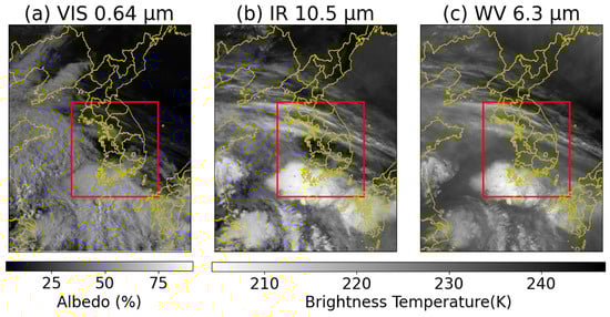
Figure 1. Examples of input dataset used for our models. GK2A satellite images of the Korean Peninsula region at 00:00 UTC on 4 May 2023. (a) VIS channel at 0.64 µm. (b) IR channel at 10.5 µm. (c) WV channel at 6.3 µm. The VIS channel is displayed as albedo (%), while both the IR and WV channels are presented as brightness temperature (K). The red box indicates the training area of our models, which corresponds to the largest region covered by the KMA radar. The entire image domain is used as the test area.

The VIS channel, with a spatial resolution of 0.5 km, provides the highest spatial detail among the AMI wavelength bands. It is particularly effective for identifying fog and cloud boundaries, overshooting tops, and small-scale convective cells. In contrast, the IR channel has a spatial resolution of 2 km, where warmer, low-altitude features appear darker and colder, high-altitude features appear brighter. This channel is widely used to monitor the evolution and displacement of cloud systems and to analyze tropical cyclones. The WV channel, also with a spatial resolution of 2 km, is mainly used to observe upper-tropospheric moisture, track typhoon trajectories, detect hazardous weather patterns, and support numerical weather prediction.

The raw pixel values from each GK2A channel are initially provided as unprocessed digital counts. To accurately interpret their physical characteristics, these values must be converted into physical quantities. Specifically, VIS channel values are converted to albedo, while IR and WV channel values are transformed into brightness temperatures. These conversions are performed using the calibration tables provided by the NMSC. Since the VIS channel is not available during nighttime, we excluded all nighttime data from the training process and only used data from 09:00 to 16:00 local time.

All data are resampled to a spatial resolution of 2 km using bilinear interpolation to ensure consistent spatial resolution across all channels. Additionally, the data are normalized to a range of [−1, 1] to improve training efficiency. Since KMA radar observations cover only a limited area, the satellite data used for model training are cropped to match the radar coverage region, as indicated by the red box (275 × 300 pixels) in Figure 1. For the testing phase, we employ the entire domain shown in Figure 1, which encompasses the full extent of the Korean Peninsula and corresponds to 576 × 720 pixels. Finally, the three spectral channels are concatenated to form the input tensors used for training the deep learning model.

The dataset spans the period from 4 May 2021, to 3 May 2023, with temporal intervals of 10 min. However, due to the intrinsic characteristics of meteorological data, non-rain samples are far more frequent than rain samples, resulting in substantial class imbalance. To mitigate this issue and ensure that the model sufficiently learns precipitation specific features, we adopted a differentiated temporal sampling strategy. Rainy periods were retained at the original 10-min resolution to capture the rapid variability of rainfall, whereas non-rain periods were downsampled to 1-h intervals to avoid excessive accumulation of non-rain cases.

2.2. KMA Weather Radar

Radar-observed data are typically obtained by volume scan measurements, and this value represents the radar reflectivity factor, Z $({\mathrm{mm}}^6/{\mathrm{m}}^3)$ [42]. It is necessary to convert Z into rainfall rate, R $(\mathrm{mm}/\mathrm{h})$, using the Z-R relationship. This relationship is expressed as follows [40]:

$$Z=a{R}^b,$$

(1)

where a and b are parameters depending on rainfall type, seasonal impact, and different topographies [43]. As these parameters can vary under different conditions, numerous studies have focused on determining appropriate values for the Z-R relationship [44,45,46,47]. In this study, we employ the Hybrid Surface Precipitation (HSP) dataset provided by the KMA as the target dataset. The HSP is derived from the Hybrid Surface Rainfall (HSR) observations and serves as a refined precipitation estimate. While several radar-based datasets are available, such as the CMAX and HSR, the HSP was selected due to its improved representativeness of precipitation. All radar based datasets, including CMAX, HSR, and HSP, have a resolution of 0.5 km.

The CMAX dataset represents composite reflectivity, defined as the maximum radar reflectivity within each vertical column across all elevation angles observed by the weather radar [48]. The HSR, on the other hand, was developed to enhance quantitative precipitation estimation (QPE) by utilizing radar reflectivity at hybrid surfaces corresponding to the lowest elevation angles, thereby minimizing beam blockage and ground clutter [49].

The HSP data further refines precipitation estimation by synthesizing HSR data from multiple radar sites and integrating dual-polarization radar variables, such as $R\left(Z\right)$, $R(Z,Z_{DR})$, and $R(Z,Z_{DR},K_{DP})$. Unlike reflectivity-based datasets (expressed in dBZ), the HSP directly provides rainfall rate (mm h⁻¹), eliminating the need for conversion using an empirical Z-R relationship. Accordingly, the HSP offers an accurate and physically meaningful target variable for model training.

2.3. GK2A Quantitative Precipitation Estimation

Precipitation estimation using infrared (IR) imagery primarily relies on the relationship between cloud-top temperature and surface rainfall rate. For example, the Geostationary Operational Environmental Satellite (GOES) Multispectral Rainfall Algorithm (GMSRA) combines observations from five spectral channels of NOAA’s GOES, including the visible (0.65 μm), near-infrared (3.9 μm), and thermal infrared window bands (11 μm and 12μm). Previous studies have shown that the GMSRA outperforms the GOES Precipitation Index (GPI), which relies on a single IR channel [50].

To further enhance satellite-based rainfall retrieval, the Enterprise Rain Rate(ERR)/Self-Calibrating Multivariate Precipitation Retrieval (SCaMPR) algorithm integrates GOES-based infrared estimates with microwave-based precipitation data over fine temporal and spatial scales [22]. The SCaMPR algorithm has demonstrated lower bias and reduced overall root mean square error (RMSE) compared to GMSRA. Building on this framework, the GOES-16 Quantitative Precipitation Estimation (QPE) algorithm adopts the SCaMPR methodology, utilizing both IR and water vapor (WV) channels. The GOES-16 QPE exhibits general consistency with the Gauge-Calibrated Multi-Radar Multi-Sensor (GC-MRMS) dataset, which serves as a ground reference. Although it effectively detects heavy precipitation, its performance is notably higher in the eastern United States than in the western region, where infrared-based sensors struggle with shallow precipitation and complex terrain.

The Korea Meteorological Administration (KMA) has also developed a satellite-based precipitation estimation product using GK2A satellite data, known as the GK2A QPE. This algorithm estimates rainfall rates using WV channels (6.24 μm, 7.34 μm) and IR channels (8.59 μm, 11.21 μm, 12.36 μm). The GK2A QPE consists of five major steps: (1) converting Advanced Meteorological Imager (AMI) radiance to brightness temperature, (2) computing brightness temperature differences (BTDs) to classify cloud types, (3) selecting a cloud database through probability density function (PDF) comparison, (4) estimating rainfall rate using Bayesian inversion calibrated with Global Precipitation Measurement (GPM) Dual-frequency Precipitation Radar (DPR) data, and (5) applying post-calibration and data storage.

Compared to ground-based radar, instantaneous rainfall estimates from GK2A QPE exhibit lower correlation and higher false alarm rates, primarily due to spatial and temporal mismatches inherent to infrared-based sensors. However, for 24-h accumulated rainfall, the correlation coefficient (CC) improves to approximately 0.8, with a probability of detection (POD) above 0.9 and a false alarm ratio (FAR) below 0.1 [41]. A comparison with GOES-16 QPE shows that GK2A QPE provides comparable detection capability. For instance, during its peak performance on 18 September 2019, GOES-16 QPE recorded a POD of 0.75 and an FAR of 0.71 [51]. However, these comparisons are not strictly equivalent due to differences in validation datasets and test periods.

To evaluate the performance of our proposed model, we compare the estimated rainfall rates against both the HSP ground truth dataset and the GK2A QPE products provided by the KMA. We conduct both quantitative and qualitative evaluations focusing on two periods: (1) a one-year period from May 2023 to April 2024 to assess overall performance, and (2) August 2023 representing the summer rainy season in Korea.

3. Method

3.1. Deep Learning Model

We adopt the Pix2PixCC model proposed by Jeong et al. [37], which is an enhanced version of Pix2PixHD [38]. Pix2PixHD extends the original Pix2Pix framework [52] to enable high-resolution image-to-image translation. However, to generate physically meaningful outputs rather than merely visually realistic ones, it is essential to consider the pixel-wise correlation between the generated images and the ground-truth data. The original Pix2PixHD framework does not explicitly account for this correlation, which limits its ability to capture physically consistent spatial structures. To overcome this limitation, Pix2PixCC introduces a correlation coefficient (CC)-based objective function that enhances the consistency between generated and real data. This addition not only improves the physical fidelity of the outputs but also yields visually realistic and statistically correlated predictions.

Pix2PixCC consists of three primary components: a generator, a discriminator, and an inspector. The generator synthesizes realistic outputs from input data, the discriminator distinguishes between real and generated pairs, and the inspector computes the correlation coefficient between the target and the generated data. Figure 2 illustrates the overall architecture of the Pix2PixCC model.

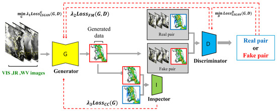
Figure 2. Architecture of the proposed model. The model consists of a generator (G), a discriminator (D), and an inspector (I), shown in yellow, blue, and green, respectively. The generator produces realistic outputs from the input data, the discriminator distinguishes between real (red box) and generated (blue box) pairs, and the inspector computes the correlation coefficient between the target and generated data.

The objective function comprises three components. First, the feature matching (FM) loss minimizes the absolute difference between feature maps of real and generated pairs across multiple discriminator layers:

$$L_{FM}(G,D)=\sum _{i=1}^T{\displaystyle \frac{1}{N_i}}|D^{\left(i\right)}(x,y)-D^{\left(i\right)}(x,G\left(x\right))|,$$

(2)

where x, y, and $G\left(x\right)$ denote the input, ground truth, and generated outputs, respectively; T represents the total number of discriminator layers, and $N_i$ is the number of pixels in the feature map of the i-th layer.

Second, we employ the least-squares generative adversarial network (LSGAN) losses [53], defined as:

$$L_{LSGAN,G}(G,D)={\displaystyle \frac{1}{2}}{(D(x,G\left(x\right))-1)}^2,$$

(3)

$$L_{LSGAN,D}(G,D)={\displaystyle \frac{1}{2}}{(D(x,y)-1)}^2+{\displaystyle \frac{1}{2}}{\left(D(x,G\left(x\right))\right)}^2$$

(4)

Finally, the CC-based loss function $L_{CC}$ measures the degree of correlation between generated and ground-truth images:

$$L_{CC}\left(G\right)=\sum _{i=0}^T{\displaystyle \frac{1}{T+1}}(1-C{C}_i(y,G\left(x\right))),$$

(5)

where $C{C}_i$ denotes the correlation coefficient between the $2^i$-times downsampled versions of y and $G\left(x\right)$.

The overall optimization objectives are expressed as:

$$\underset{G}{\min }{\lambda }_1{L}_{LSGAN,G}(G,D)+{\lambda }_2{L}_{FM}(G,D)+{\lambda }_3{L}_{CC}\left(G\right),$$

(6)

$$\underset{D}{\min }{L}_{LSGAN,D}(G,D),$$

(7)

where ${\lambda }_1$, ${\lambda }_2$, and ${\lambda }_3$ are hyperparameters that control the relative weights of the loss terms. In this study, ${\lambda }_1$, ${\lambda }_2$, and ${\lambda }_3$ are set to 2, 10, and 5, respectively, based on the settings suggested by Jeong et al. [37]. The GAN loss term (${\lambda }_1$) is assigned a smaller weight of 2 to mitigate instability during adversarial training, whereas the FM loss (${\lambda }_2$) receives the largest weight of 10 to promote structural consistency and stable convergence. The CC loss (${\lambda }_3$) is empirically set to 5, as this configuration yielded the best correlation and visual fidelity between generated and real data.

While Model-HSP utilizes HSP radar data as its target, the baseline Model-CMX was trained using CMAX radar data. Figure 3 compares rainfall rate estimates from Model-HSP and Model-CMX against the HSP ground truth. Model-CMX effectively reproduces radar reflectivity patterns, showing strong detection of light rainfall (<1 mm h⁻¹); however, its accuracy degrades significantly under heavy rainfall conditions, often leading to intensity underestimation and high false alarm rates. In contrast, Model-HSP slightly overestimates precipitation but more accurately reproduces the spatial distribution and intensity of heavy rainfall. To exploit the complementary characteristics of the two models and improve accuracy across different rainfall intensities, an ensemble strategy is adopted.

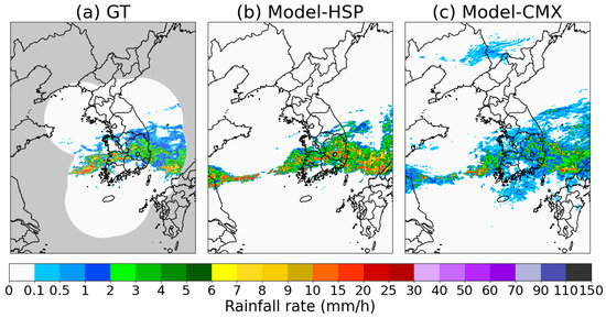
Figure 3. Comparison of GT (HSP radar), Model-HSP, and Model-CMX rainfall rate estimates. (a) GT (HSP radar), (b) Model-HSP, and (c) Model-CMX at 00:30 UTC on 29 May 2023. Model-HSP performs better in regions of heavy rainfall, while Model-CMX performs better in capturing lighter rainfall.

The model was trained on an NVIDIA RTX A6000 GPU using the PyTorch (version 2.1) deep learning framework with CUDA 11.4 support. The Adam optimizer [54] was used with a learning rate of 2 × 10⁻⁴. Training was conducted for 500 epochs with a batch size of 8, requiring approximately 44 h to complete. A learning rate decay was applied starting from epoch 151, with the learning rate was gradually decreased at each epoch for both the generator and discriminator optimizers. Model checkpoints were evaluated using multiple performance metrics, and the best-performing model was selected for rainfall map generation. During inference, the trained model generated predictions for 15,443 input–target pairs in approximately 15 min.

3.2. Ensemble Approach

To further enhance rainfall estimation performance, we adopt a learning-based ensemble approach, referred to as Model-ENS. Unlike heuristic or manually weighted combinations, Model-ENS integrates the outputs of Model-CMX and Model-HSP through supervised learning, allowing the ensemble weights to be adaptively learned from data. Specifically, Model-ENS is implemented using a multi-layer perceptron (MLP) with two hidden layers. The inputs to the MLP are the pixel-wise rainfall estimates generated by Model-CMX and Model-HSP, while the target output is the ground-truth HSP data. The ensemble model is trained over the same training period as the base models, enabling it to learn an optimal nonlinear mapping that combines the complementary strengths of the two models under varying rainfall conditions.

Through this learning process, Model-ENS effectively exploits the high detection capability of Model-CMX for light rainfall and the superior intensity representation of Model-HSP for heavy rainfall, resulting in improved accuracy and robustness across different precipitation regimes. Detailed evaluations of Model-ENS are presented in Section 4.

3.3. Evaluation Framework

We evaluate the performance of our deep learning model using multiple quantitative metrics, including the root mean square error (RMSE) and correlation coefficient (CC), to assess the accuracy and consistency of rainfall estimation. The evaluation is conducted over two periods—a one-year span from May 2023 to April 2024 and the August 2023 monsoon season. RMSE quantifies the average deviation between the predicted and ground-truth values; thus, a lower RMSE indicates better agreement between prediction and observation. The CC measures the linear correlation between predicted and reference values, where values closer to 1 denote stronger agreement. These metrics are defined as follows:

$$RMSE=\sqrt{{\displaystyle \frac{1}{N}}\sum _{i=1}^N{(X_i-Y_i)}^2},$$

(8)

$$CC={\displaystyle \frac{{\sum }_{i=1}^N(X_i-\overline{X})(Y_i-\overline{Y})}{\sqrt{{\sum }_{i=1}^N{(X_i-\overline{X})}^2{\sum }_{i=1}^N{(Y_i-\overline{Y})}^2}}},$$

(9)

where $X_i$ and $Y_i$ represent the ground-truth and predicted rainfall rates, $\overline{X}$ and $\overline{Y}$ are their respective mean values, and N is the total number of pixels.

In addition to RMSE and CC, we employ categorical verification metrics—probability of detection (POD), false alarm ratio (FAR), critical success index (CSI), and fractions skill score (FSS)—to evaluate the model’s ability to detect rainfall events of varying intensities. These metrics are analyzed at thresholds of 0.1, 1, and 5 mm h⁻¹. They are defined as follows:

$$POD={\displaystyle \frac{TP}{TP+FN}},$$

(10)

$$FAR={\displaystyle \frac{FP}{FP+TP}},$$

(11)

$$CSI={\displaystyle \frac{TP}{TP+FN+FP}}$$

(12)

FSS quantifies the spatial correspondence between predicted and observed rainfall fields using pixel-wise comparisons and is defined as:

$$FSS=1-{\displaystyle \frac{{\sum }_N{(P_{fcst}-P_{obs})}^2}{{\sum }_N(P_{fcst}^2+P_{obs}^2)}},$$

(13)

where $P_{fcst}$ and $P_{obs}$ denote the fractional forecast and observed rain areas, respectively, and N is the total number of pixels.

POD, FAR, and CSI are computed based on the contingency table summarized in Table 2. True positives (TPs) and true negatives (TNs) correspond to the numbers of pixels correctly identified as rain and no-rain, respectively. False positives (FPs) represent pixels incorrectly predicted as rain when no rainfall occurred, whereas false negatives (FNs) indicate missed detections where rainfall was present but not predicted.

Table 2. Contingency table of our study.

Contingency Table		Observation
		Rain	No-Rain
Prediction	Rain	True Positive (TP)	False Positive (FP)
	No-rain	False Negative (FN)	True Negative (TN)

In addition to satellite based validation using GK2A satellite-derived rainfall and radar observations, we further evaluate the performance of Model-HSP, Model-CMX, and Model-ENS by comparing their one hour accumulated rainfall estimates with ground based measurements from Automatic Weather Stations (AWS). Since our models are trained on remote sensing data, AWS measurements are incorporated as an independent validation source to verify consistency with actual ground conditions, in addition to satellite and radar based patterns. Figure 4 presents the spatial distribution of 727 AWS stations across the Korean Peninsula, providing comprehensive ground truth coverage for evaluation.

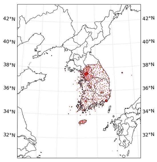
Figure 4. Locations of AWS observations on the Korean Peninsula.

Furthermore, to evaluate the models’ capability in reproducing realistic precipitation structures, we conduct case-based analyses for representative summertime rainfall events over Korea. These analyses assess how well each model captures the spatial distribution of rainfall and the overall organization of the precipitation system. Through these case studies, we examine whether the estimated rainfall fields faithfully represent the characteristic patterns observed during major summer precipitation episodes.

4. Result

We evaluated Model-HSP and Model-ENS by comparing their performance against Model-CMX and the GK2A QPE over two distinct periods: (1) a one-year period from May 2023 to April 2024 to assess overall performance and (2) August 2023 to analyze model behavior during the summer monsoon season in Korea. The evaluation was conducted at spatial resolutions of 2 km and 4 km using RMSE and CC as quantitative metrics.

4.1. Parameter Analysis Results

Since Model-CMX produces rainfall estimates in the form of reflectivity, it is essential to assess the sensitivity of the final precipitation retrieval to the choice of Z-R relationships. To ensure that the reflectivity to rainfall conversion does not introduce unintended biases, we conducted a series of experiments on our test dataset using five commonly referenced Z-R formulations: $Z=200R^{1.6}$, $Z=204R^{1.7}$, $Z=224R^{1.54}$, $Z=250R^{1.5}$, and $Z=255R^{1.45}$. By applying these different combinations of coefficients (a) and exponents (b), we evaluated their impact on quantitative precipitation estimation performance. Among the tested relationships, the parameter pair $a=204$ and $b=1.7$ achieved the best overall results, outperforming the widely used Marshall–Palmer formulation ($a=200$, $b=1.6$). This optimal Z-R relationship was subsequently adopted to enhance the robustness and reliability of the rainfall estimates used in the ensemble configuration.

After determining the optimal Z-R relationship, the ensemble configuration was finalized using the learning-based framework described in Section 3. In this step, the reflectivity outputs from Model-CMX were first converted into rainfall rates using the selected Z-R relationship. This conversion was adopted because experiments showed that using Z-R derived rainfall estimates from Model-CMX led to better ensemble performance than directly using raw reflectivity values.

The learning-based ensemble was implemented using a multi-layer perceptron (MLP) with two hidden layers consisting of 64 and 32 nodes. The MLP was trained using the rainfall estimates from Model-HSP and the Z-R–converted Model-CMX outputs as inputs, with the HSP data as the target. This configuration allows the ensemble to adaptively combine information from both models under different rainfall conditions. Together with the optimal Z-R relationship, this learning-based ensemble setup is used for all subsequent performance evaluations, ensuring that the comparative results presented in later sections are based on a consistently calibrated and robust model configuration.

Table 3 presents a quantitative comparison of Model-HSP, Model-ENS, Model-CMX, GK2A QPE, and the U-Net model in terms of RMSE and CC at spatial resolutions of 2 km and 4 km, evaluated for August 2023 and for the one year period from May 2023 to April 2024. Values in parentheses indicate CC computed on a logarithmic scale. For the one year evaluation, Model-ENS consistently achieves the lowest RMSE at both spatial resolutions, demonstrating superior error reduction compared to all other models. At 4 km resolution, Model-ENS records an RMSE of 2.71 mm/h with a CC of 0.24 (0.27 in logarithmic scale), outperforming Model-HSP, Model-CMX, GK2A QPE, and the U-Net model. While the U-Net model exhibits relatively high CC values, its RMSE remains substantially higher, indicating smoother but less accurate rainfall estimates. GK2A QPE shows the weakest overall performance, with higher RMSE and lower CC across all cases. During August 2023, all models exhibit increased RMSE values along with higher CC, reflecting the localized and intense nature of summer rainfall. Under these conditions, Model-ENS again demonstrates robust performance, achieving the lowest RMSE at 4 km resolution (5.03 mm/h) and a high logarithmic CC of 0.37. These results confirm that the proposed ensemble model provides improved accuracy and consistency across both long term and event focused evaluation periods.

Table 3. Comparison of Model-HSP, Model-ENS, Model-CMX, the U-Net model, and the GK2A QPE at spatial resolutions of 2 km and 4 km for August 2023 and the period from May 2023 to April 2024. Values shown in parentheses correspond to results computed on a logarithmic scale. Note: Bold indicates the best-performing results among the compared methods.

Period	Resolution	Model-HSP		Model-ENS		Model-CMX		GK2A QPE		Unet
		RMSE (mm/h)	CC (log)	RMSE (mm/h)	CC (log)	RMSE (mm/h)	CC (log)	RMSE (mm/h)	CC (log)	RMSE (mm/h)	CC (log)
May 2023	2 km	6.27	0.14 (0.14)	3.43	0.21 (0.25)	3.87	0.19 (0.25)	4.88	0.05 (0.06)	4.25	0.24 (0.27)
April 2024	4 km	4.89	0.16 (0.16)	2.71	0.24 (0.27)	2.99	0.23 (0.27)	3.69	0.05 (0.07)	3.41	0.27 (0.27)
August 2023	2 km	10.59	0.19 (0.19)	6.92	0.27 (0.32)	7.92	0.24 (0.32)	8.47	0.09 (0.11)	8.02	0.32 (0.34)
	4 km	7.96	0.23 (0.23)	5.03	0.32 (0.37)	5.65	0.30 (0.36)	6.24	0.08 (0.11)	5.92	0.38 (0.37)

Figure 5 shows the performance diagram of rainfall detection skills for August 2023 at thresholds of 0.1, 1, and 5 mm/h. At the 0.1 mm/h threshold, Model-ENS and Model-CMX exhibit the highest POD values, located in the upper region of the diagram. Model-ENS shows a relatively higher success ratio (SR) than Model-CMX, while Model-HSP demonstrates a moderate POD with the highest SR, indicating the lowest FAR. In contrast, GK2A QPE exhibits a relatively high POD but a low SR, placing it toward the left side of the diagram. At the 1 mm/h threshold, Model-ENS achieves the highest POD, whereas Model-CMX shows slightly lower POD with comparable SR. Model-HSP exhibits intermediate performance, while GK2A QPE remains clustered in the lower-left region with low POD and SR values. When the threshold increases to 5 mm/h, the performance of all models degrades, reflecting the increased difficulty of detecting heavier rainfall. Model-HSP shows slightly higher POD, while Model-CMX attains the highest SR. Model-ENS exhibits moderate values for both POD and SR. GK2A QPE again shows the weakest performance. Overall, these results demonstrate that Model-ENS integrates complementary information from Model-HSP and Model-CMX, leading to improved quantitative accuracy and spatial representation compared to existing satellite based precipitation estimation methods.

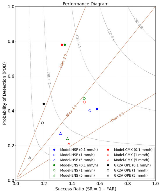
Figure 5. Performance diagram of the rainfall detection skills. Blue, red, green, and black markers represent Model-HSP, Model-CMX, Model-ENS, and the GK2A QPE, respectively. Metrics are calculated at rainfall thresholds of 0.1, 1, and 5 mm/h during August 2023, using HSP rainfall rate as ground truth. The spatial resolution is 2 km.

We further evaluate the performance of Model-HSP, Model-CMX, and Model-ENS by comparing their one-hour accumulated rainfall estimates with ground-based observations from Automatic Weather Stations (AWS).

Figure 6 presents time series comparisons of daily rainfall rates between the three models and AWS observations during the summer period (June to September 2023). As shown in Figure 6a, all models capture the temporal variations of daily mean rainfall and show good agreement with AWS observations. The timing of rainfall events is consistent between the models and observations, particularly during active precipitation periods in early July and mid August, corresponding to the summer rainy season. Figure 6b shows the daily maximum rainfall rates. While all models reproduce the overall temporal variability, peak rainfall intensities are systematically underestimated. Among the models, Model-CMX occasionally produces higher peak values than Model-HSP and Model-ENS, but still underestimates the magnitude of major rainfall events. These results indicate that, although the models effectively represent the temporal evolution of rainfall, limitations remain in capturing extreme precipitation intensities observed by AWS.

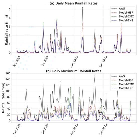
Figure 6. Time series comparison between our models and AWS observations. (a) Daily mean rainfall rates and (b) daily maximum rainfall rates. Both are based on 1-h accumulated rainfall from June to September 2023.

4.2. Case Study

To further assess the spatial and temporal representativeness of the models, three rainfall events were selected for qualitative evaluation: (1) Typhoon Khanun, (2) a summer monsoon system, and (3) a convective rainfall event. Figure 7, Figure 8 and Figure 9 illustrate the results for these cases at 00:00, 02:00, 04:00, and 06:00 UTC.

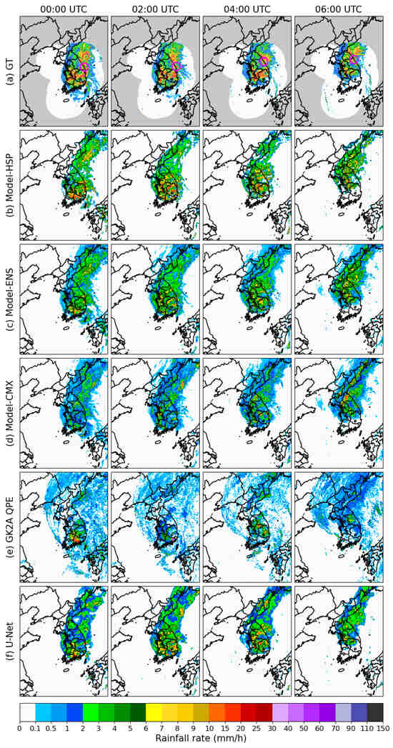
Figure 7. Comparison of rainfall maps for Case 1 (Typhoon Khanun). (a) GT (HSP ground truth), (b) Model-HSP, (c) Model-ENS, (d) Model-CMX, (e) GK2A QPE, and (f) U-Net model on 10 August 2023, at 00:00, 02:00, 04:00, and 06:00 UTC. The pink circle indicates the location of the maximum rainfall rate in GT.

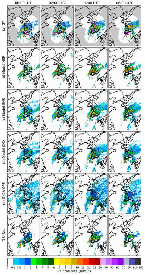
Figure 8. Same as Figure 7 but for Case 2 (Monsoon) on 18 July 2023.

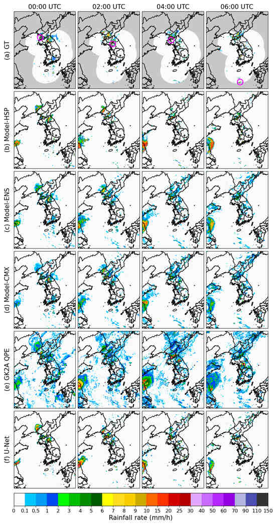
Figure 9. Same as Figure 7 but for Case 3 (Convective rainfall) on 26 July 2023.

4.2.1. Typhoon Khanun (10 August 2023)

Figure 7 compares the rainfall distributions estimated by each model with the HSP ground truth and the GK2A QPE during Typhoon Khanun. Model-HSP (panel b) successfully captures the overall spatial structure and intensity of the typhoon, but fails to reproduce light rainfall (<1 mm/h) in the peripheral regions. Model-ENS (panel c) provides the most accurate representation of rainfall intensity and spatial distribution, effectively reproducing both the typhoon core and outer rainbands with strong temporal consistency. In particular, the model shows high fidelity in the 2 to 5 mm/h rainfall range, capturing light to moderate precipitation with improved accuracy. Model-CMX (panel d) captures the general storm structure but underestimates rainfall intensity, with most values below 2 mm/h. The GK2A QPE (panel e) further underestimates rainfall intensity while overestimating the spatial extent of precipitation. The U-Net model (panel f) produces a smoother and more diffused rainfall pattern, resulting in blurred boundaries and a loss of fine-scale features. Although the overall structure of is represented, localized variations within the rainbands are not adequately captured. This comparison indicates that Model-ENS shows the highest agreement with the HSP observations, accurately reflecting the spatial coherence of typhoon induced rainfall. Remaining underestimations in heavy rainfall regions likely stem from the limited number of extreme rainfall cases in the training dataset and the complex topography of the Korean Peninsula. Incorporating topographic information as auxiliary inputs represents a promising direction for future research. In addition, the satellite based framework enables rainfall estimation in regions beyond the coverage of ground based radar observations.

4.2.2. Monsoon Rainfall (18 July 2023)

Figure 8 shows the model results for a summer monsoon event over the Korean Peninsula. All models capture the evolution of the monsoon front and preserve the overall structural of the rainfall system. Model-HSP accurately represents heavy rainfall between 00:00 and 02:00 UTC but slightly overestimates intensity along the west coast at 04:00 UTC. Model-ENS maintains strong spatial continuity and realistic temporal evolution of the rainband and closely matching the HSP observations in both intensity and location. Model-CMX tends to overestimate the spatial coverage of light precipitation, while GK2A QPE exaggerates rainfall extent in non-rain areas and fails to reproduce fine-scale structures such as the inverted U-shaped band observed at 02:00 UTC. The U-Net model shows a blurred rainfall pattern and does not accurately capture weaker precipitation over the ocean. These results indicate that Model-ENS provides the most reliable reconstruction of the monsoon rainfall field, with reduced overestimation and fragmentation compared to the other models.

4.2.3. Convective Rainfall (26 July 2023)

Figure 9 presents a short lived convective rainfall event characterized by localized, high-intensity precipitation. Accurately modeling such events is challenging due to their rapid evolution and small spatial scales. Both Model-HSP and Model-ENS capture the spatial locations of convective cores at 00:00 UTC, showing good agreement with the HSP ground truth. Model-ENS further improves spatial accuracy over the southern peninsula, maintaining concentrated rainfall structures across subsequent time steps. In contrast, Model-CMX fails to detect localized convective centers, instead generating diffuse and weak rainfall patterns. GK2A QPE exhibits the largest discrepancies, substantially overestimating the areal extent of rainfall and frequently predicting spurious precipitation where none is observed. The U-Net model generally captures the overall spatial distribution and major structural features of convective rainfall. However, it shows limitations in accurately reproducing light-to-moderate rainfall intensity of approximately 1 to 2 mm/h. These findings highlight the superior ability of Model-ENS to capture small-scale, high-intensity convective rainfall, reflecting improved spatial precision and physical consistency relative to other models.

Table 4 summarizes the RMSE and CC values for Model-HSP, Model-ENS, Model-CMX, GK2A QPE, and the U-Net model across three representative rainfall cases—Typhoon Khanun, the summer monsoon, and localized convective rainfall evaluated at spatial resolutions of 2 km and 4 km. Overall, Model-ENS consistently exhibits superior performance across all cases and spatial resolutions. At 4 km resolution, Model-ENS achieves the lowest RMSE values of 6.11 mm/h, 6.24 mm/h, and 9.49 mm/h for Case 1 (Typhoon Khanun), Case 2 (Monsoon), and Case 3 (Convective rainfall), respectively. In terms of correlation, Model-ENS also records high CC values, with logarithmic CCs of 0.47, 0.50, and 0.41 for Case 1, Case 2, and Case 3, respectively. However, for Case 3, the U-Net model yields the highest CC, achieving values of 0.40 and 0.44 at 2 km and 4 km resolutions, respectively, which may be partly attributed to the spatial smoothing effect of the U-Net architecture.

Table 4. Comparison of Model-HSP, Model-ENS, Model-CMX, the U-Net model, and the GK2A QPE for three representative rainfall cases at spatial resolutions of 2 km and 4 km. Case 1 corresponds to Typhoon Khanun on 10 August 2023; Case 2 to a summer monsoon event over the Korean Peninsula on 18 July 2023; and Case 3 to a localized convective rainfall event on 26 July 2023. Values are computed on a logarithmic scale. Note: Bold indicates the best-performing results among the compared methods.

Period	Resolution	Model-HSP		Model-ENS		Model-CMX		GK2A QPE		U-Net
		RMSE (mm/h)	CC (log)	RMSE (mm/h)	CC (log)	RMSE (mm/h)	CC (log)	RMSE (mm/h)	CC (log)	RMSE (mm/h)	CC (log)
Case 1	2 km	7.36	0.21 (0.28)	6.52	0.32 (0.43)	7.18	0.19 (0.40)	8.61	0.02 (0.11)	6.83	0.32 (0.47)
	4 km	6.75	0.25 (0.32)	6.11	0.36 (0.47)	6.77	0.23 (0.44)	7.97	0.04 (0.17)	6.45	0.34 (0.49)
Case 2	2 km	9.48	0.25 (0.28)	7.10	0.34 (0.47)	7.61	0.28 (0.44)	8.45	0.15 (0.19)	8.01	0.37 (0.44)
	4 km	8.39	0.27 (0.30)	6.24	0.38 (0.50)	6.67	0.33 (0.47)	7.20	0.21 (0.22)	7.14	0.40 (0.44)
Case 3	2 km	15.10	0.23 (0.16)	12.59	0.28 (0.37)	13.10	0.23 (0.39)	13.36	0.07 (0.11)	12.93	0.40 (0.37)
	4 km	12.38	0.23 (0.19)	9.49	0.35 (0.41)	9.85	0.27 (0.40)	10.79	0.07 (0.13)	9.74	0.44 (0.38)

These results clearly demonstrate the robustness of the ensemble approach. By effectively integrating the complementary strengths of Model-HSP, which captures heavy rainfall intensity, and Model-CMX, which provides superior detection of light precipitation, Model-ENS achieves improved accuracy and stability across diverse precipitation regimes. This confirms the potential of the ensemble model as a reliable framework for satellite based quantitative precipitation estimation in complex meteorological environments.

5. Discussion

The results presented in this study demonstrate that the proposed ensemble model (Model-ENS) provides substantial improvements in satellite-based quantitative precipitation estimation (QPE) compared to existing methods. By combining the complementary advantages of Model-HSP, which is trained using direct precipitation values and effectively captures heavy rainfall, and Model-CMX, which is trained using radar reflectivity (CMAX) data and shows strong sensitivity to light precipitation, Model-ENS achieves consistently improved performance across diverse rainfall scenarios, including typhoon, monsoon, and convective events.

Compared with the operational GK2A QPE product, the ensemble model exhibits higher correlation coefficients and lower RMSE values across all spatial resolutions. Notably, the improvement is most significant for convective rainfall cases, where infrared-based methods often struggle due to weak relationships between cloud-top temperature and surface precipitation. These results suggest that the learning based ensemble framework is able to capture nonlinear relationships between satellite observations and near surface rainfall, thereby compensating for limitations inherent in physically based retrieval approaches.

Despite these advancements, certain limitations remain, particularly with respect to the representation of extreme rainfall. The proposed model tends to underestimate high-intensity precipitation, especially in mountainous regions and during typhoon events. This limitation can be attributed to the relatively small number of extreme rainfall samples in the training dataset, as well as the exclusion of auxiliary geophysical and atmospheric variables—such as terrain elevation and humidity—that play important roles in precipitation formation.

Beyond these data-related factors, the underestimation of extreme rainfall may also be associated with inherent characteristics of GAN-based architectures. Because adversarial training emphasizes dominant patterns in the training distribution, rare high-intensity rainfall events can be underrepresented during the learning process. As a result, the model may produce smoother and more conservative rainfall estimates during extreme precipitation episodes. Future work should therefore focus on refining the learning objectives and training strategies, including the incorporation of loss-function-based approaches that explicitly emphasize extreme rainfall, with the goal of better preserving the statistical and physical characteristics of high-impact precipitation events.

Another important limitation arises from the characteristics of the radar datasets used for model training. CMAX and HSP fundamentally differ in their data representations, with reflectivity and converted rainfall rates, respectively, which complicates their direct integration without careful preprocessing and harmonization. Although multi radar training was not explored in this study, extending the training dataset to include radar systems with different Z R relationships could improve model generalization by exposing it to a wider range of precipitation characteristics. This highlights the need for future research on systematic harmonization strategies that enable robust multi radar learning.

We further examined the contribution of the visible channel by conducting an additional experiment in which it was excluded to enable continuous day and night operation. The use of visible channel information represents a deliberate design choice aimed at leveraging its strong capability to capture cloud structure during daytime conditions, enabling stable, high-temporal-resolution rainfall monitoring at 10-min intervals. As expected, removing the visible channel resulted in a moderate degradation in CSI, POD, and FAR. Nevertheless, the overall performance remained stable across the diurnal cycle, without introducing noticeable discontinuities between daytime and nighttime conditions. Importantly, even under this visible independent configuration, the proposed framework consistently outperformed the operational GK2A QPE, indicating that it retains meaningful predictive skill throughout both daytime and nighttime periods. These results suggest that, while visible channel information enhances daytime rainfall estimation, the proposed framework can be configured for different operational settings depending on input availability. In this sense, the visible-based and visible-free configurations can be regarded as complementary options, reflecting a trade-off between enhanced daytime accuracy and continuous all-day operation.

To address the aforementioned limitations, future work should focus on several key directions. The training dataset should be expanded to encompass a wider range of meteorological conditions, and auxiliary geophysical variables—such as terrain elevation (DEM), moisture indices, and wind fields—should be incorporated as additional inputs to address the current limitations. Given that the Korean Peninsula is characterized by complex and mountainous terrain, such topographic features can substantially influence the spatial distribution of precipitation. Incorporating DEM data as an additional input channel is therefore expected to help the model more effectively capture orographic rainfall effects, thereby improving rainfall estimation accuracy in mountainous and topographically complex regions. In addition, future research should focus on reducing reliance on visible channel information while preserving the accuracy achieved under VIS-enabled conditions. Improving VIS-independent performance will be key to enhancing the robustness applicability of satellite-based precipitation estimation.

Finally, extending the model to an operational real-time system by utilizing streaming satellite data would enable its application to nowcasting of heavy rainfall and flood risk management.

6. Summary and Conclusions

This study introduced a deep learning-based framework for quantitative precipitation estimation (QPE) using GK2A geostationary satellite imagery. The proposed baseline model, Model-HSP, is built upon the Pix2PixCC architecture and directly estimates rainfall rates from multi-channel satellite data trained against HSP ground-truth observations. To further enhance performance, we developed an ensemble approach, Model-ENS, that integrates the complementary outputs of Model-HSP and Model-CMX.

Comprehensive evaluations conducted over one-year and summer-season periods, as well as for representative rainfall cases—Typhoon Khanun, monsoon, and convective events—demonstrate that the proposed models can accurately estimate rainfall solely from satellite observations. The main findings of this study are as follows. First, our models successfully estimated rainfall directly from satellite imagery without relying on radar-based post-processing. This represents a significant advancement in satellite-only quantitative precipitation estimation (QPE), enabling rainfall estimation in areas where ground-based radar observations are unavailable. Second, both Model-HSP and Model-ENS consistently outperformed the GK2A QPE in terms of statistical accuracy. Among them, Model-ENS showed the best overall performance. Third, case studies confirmed that Model-ENS provided superior spatial and temporal representations of rainfall systems. This includes improvements in the representation of structure, location, and intensity, particularly in typhoon and convective rainfall scenarios.

Overall, these findings demonstrate that the proposed framework enables reliable rainfall estimation solely from satellite observations, independent of radar-derived corrections. The proposed framework was primarily evaluated using daytime observations, as it leverages visible channel information. Nighttime experiments showed a moderate degradation in performance, but the proposed framework still outperformed the operational GK2A QPE, indicating its robustness and practical applicability across the diurnal cycle. Our approach offers several advantages. By directly estimating rainfall from satellite imagery, the proposed models support near–real-time monitoring with minimal dependence on ground-based infrastructure. Moreover, the method is globally scalable and can be applied to other geostationary satellites, such as NOAA’s GOES-R series and EUMETSAT’s Meteosat Third Generation, enabling cross-regional deployment.

In conclusion, this study demonstrates the potential of deep learning and ensemble-based approaches to advance satellite-based QPE. The proposed framework not only improves the spatial and temporal consistency of rainfall estimates but also provides a scalable and practical solution for real-time precipitation monitoring in data-sparse regions.

References

- Dastane, N. Effective Rainfall in Irrigated Agriculture; CABI: Wallingford, UK, 1974. [Google Scholar]
- Sinclair, S.; Pegram, G. Combining radar and rain gauge rainfall estimates using conditional merging. Atmos. Sci. Lett. 2005, 6, 19–22. [Google Scholar] [CrossRef]
- Krajewski, W.; Smith, J.A. Radar hydrology: Rainfall estimation. Adv. Water Resour. 2002, 25, 1387–1394. [Google Scholar] [CrossRef]
- Ochoa-Rodriguez, S.; Wang, L.P.; Willems, P.; Onof, C. A review of radar-rain gauge data merging methods and their potential for urban hydrological applications. Water Resour. Res. 2019, 55, 6356–6391. [Google Scholar] [CrossRef]
- Herzegh, P.H.; Jameson, A.R. Observing precipitation through dual-polarization radar measurements. Bull. Am. Meteorol. Soc. 1992, 73, 1365–1376. [Google Scholar] [CrossRef]
- Anagnostou, E.N.; Krajewski, W.F. Real-time radar rainfall estimation. Part I: Algorithm formulation. J. Atmos. Ocean. Technol. 1999, 16, 189–197. [Google Scholar] [CrossRef]
- Germann, U.; Boscacci, M.; Clementi, L.; Gabella, M.; Hering, A.; Sartori, M.; Sideris, I.V.; Calpini, B. Weather radar in complex orography. Remote Sens. 2022, 14, 503. [Google Scholar] [CrossRef]
- Berne, A.; Krajewski, W.F. Radar for hydrology: Unfulfilled promise or unrecognized potential? Adv. Water Resour. 2013, 51, 357–366. [Google Scholar] [CrossRef]
- Rico-Ramirez, M.A.; Cluckie, I.D. Classification of ground clutter and anomalous propagation using dual-polarization weather radar. IEEE Trans. Geosci. Remote Sens. 2008, 46, 1892–1904. [Google Scholar] [CrossRef]
- Schmit, T.J.; Gunshor, M.M.; Menzel, W.P.; Gurka, J.J.; Li, J.; Bachmeier, A.S. Introducing the next-generation Advanced Baseline Imager on GOES-R. Bull. Am. Meteorol. Soc. 2005, 86, 1079–1096. [Google Scholar] [CrossRef]
- Holmlund, K.; Grandell, J.; Schmetz, J.; Stuhlmann, R.; Bojkov, B.; Munro, R.; Lekouara, M.; Coppens, D.; Viticchie, B.; August, T.; et al. Meteosat Third Generation (MTG): Continuation and innovation of observations from geostationary orbit. Bull. Am. Meteorol. Soc. 2021, 102, E990–E1015. [Google Scholar] [CrossRef]
- Yang, J.; Zhang, Z.; Wei, C.; Lu, F.; Guo, Q. Introducing the new generation of Chinese geostationary weather satellites, Fengyun-4. Bull. Am. Meteorol. Soc. 2017, 98, 1637–1658. [Google Scholar] [CrossRef]
- Bessho, K.; Date, K.; Hayashi, M.; Ikeda, A.; Imai, T.; Inoue, H.; Kumagai, Y.; Miyakawa, T.; Murata, H.; Ohno, T.; et al. An introduction to Himawari-8/9—Japan’s new-generation geostationary meteorological satellites. J. Meteorol. Soc. Jpn. Ser. II 2016, 94, 151–183. [Google Scholar] [CrossRef]
- Kim, D.; Gu, M.; Oh, T.H.; Kim, E.K.; Yang, H.J. Introduction of the advanced meteorological imager of Geo-Kompsat-2a: In-orbit tests and performance validation. Remote Sens. 2021, 13, 1303. [Google Scholar] [CrossRef]
- Huffman, G.J.; Bolvin, D.T.; Nelkin, E.J.; Wolff, D.B.; Adler, R.F.; Gu, G.; Hong, Y.; Bowman, K.P.; Stocker, E.F. The TRMM Multisatellite Precipitation Analysis (TMPA): Quasi-Global, Multiyear, Combined-Sensor Precipitation Estimates at Fine Scales. J. Hydrometeorol. 2007, 8, 38–55. [Google Scholar] [CrossRef]
- Hou, A.Y.; Kakar, R.K.; Neeck, S.; Azarbarzin, A.A.; Kummerow, C.D.; Kojima, M.; Oki, R.; Nakamura, K.; Iguchi, T. The Global Precipitation Measurement Mission. Bull. Am. Meteorol. Soc. 2014, 95, 701–722. [Google Scholar] [CrossRef]
- Sun, Q.; Miao, C.; Duan, Q.; Ashouri, H.; Sorooshian, S.; Hsu, K.L. A review of global precipitation data sets: Data sources, estimation, and intercomparisons. Rev. Geophys. 2018, 56, 79–107. [Google Scholar] [CrossRef]
- Nguyen, P.; Ombadi, M.; Sorooshian, S.; Hsu, K.; AghaKouchak, A.; Braithwaite, D.; Ashouri, H.; Thorstensen, A.R. The PERSIANN family of global satellite precipitation data: A review and evaluation of products. Hydrol. Earth Syst. Sci. 2018, 22, 5801–5816. [Google Scholar] [CrossRef]
- Kidd, C.; Levizzani, V. Status of satellite precipitation retrievals. Hydrol. Earth Syst. Sci. 2011, 15, 1109–1116. [Google Scholar] [CrossRef]
- Kidd, C.; Levizzani, V. Chapter 6—Satellite rainfall estimation. In Rainfall; Morbidelli, R., Ed.; Elsevier: Amsterdam, The Netherlands, 2022; pp. 135–170. [Google Scholar] [CrossRef]
- Liu, C.; Zipser, E.J. The global distribution of largest, deepest, and most intense precipitation systems. Geophys. Res. Lett. 2015, 42, 3591–3595. [Google Scholar] [CrossRef]
- Kuligowski, R.J. A self-calibrating real-time GOES rainfall algorithm for short-term rainfall estimates. J. Hydrometeorol. 2002, 3, 112–130. [Google Scholar] [CrossRef]
- Aonashi, K.; Awaka, J.; Hirose, M.; Kozu, T.; Kubota, T.; Liu, G.; Shige, S.; Kida, S.; Seto, S.; Takahashi, N.; et al. GSMaP passive microwave precipitation retrieval algorithm: Algorithm description and validation. J. Meteorol. Soc. Jpn. Ser. II 2009, 87, 119–136. [Google Scholar] [CrossRef]
- Kubota, T.; Shige, S.; Hashizume, H.; Aonashi, K.; Takahashi, N.; Seto, S.; Hirose, M.; Takayabu, Y.N.; Ushio, T.; Nakagawa, K.; et al. Global precipitation map using satellite-borne microwave radiometers by the GSMaP project: Production and validation. IEEE Trans. Geosci. Remote Sens. 2007, 45, 2259–2275. [Google Scholar] [CrossRef]
- Joyce, R.J.; Janowiak, J.E.; Arkin, P.A.; Xie, P. CMORPH: A method that produces global precipitation estimates from passive microwave and infrared data at high spatial and temporal resolution. J. Hydrometeorol. 2004, 5, 487–503. [Google Scholar] [CrossRef]
- Liu, Z. Comparison of integrated multisatellite retrievals for GPM (IMERG) and TRMM multisatellite precipitation analysis (TMPA) monthly precipitation products: Initial results. J. Hydrometeorol. 2016, 17, 777–790. [Google Scholar] [CrossRef]
- Huffman, G.J.; Bolvin, D.T.; Braithwaite, D.; Hsu, K.L.; Joyce, R.J.; Kidd, C.; Nelkin, E.J.; Sorooshian, S.; Stocker, E.F.; Tan, J.; et al. Integrated multi-satellite retrievals for the global precipitation measurement (GPM) mission (IMERG). In Satellite Precipitation Measurement; Springer International Publishing: Cham, Switzerland, 2020; Volume 1, pp. 343–353. [Google Scholar]
- Chen, H.; Chandrasekar, V.; Cifelli, R.; Xie, P. A machine learning system for precipitation estimation using satellite and ground radar network observations. IEEE Trans. Geosci. Remote Sens. 2019, 58, 982–994. [Google Scholar] [CrossRef]
- Sadeghi, M.; Asanjan, A.A.; Faridzad, M.; Nguyen, P.; Hsu, K.; Sorooshian, S.; Braithwaite, D. PERSIANN-CNN: Precipitation estimation from remotely sensed information using artificial neural networks–convolutional neural networks. J. Hydrometeorol. 2019, 20, 2273–2289. [Google Scholar] [CrossRef]
- Moraux, A.; Dewitte, S.; Cornelis, B.; Munteanu, A. Deep learning for precipitation estimation from satellite and rain gauges measurements. Remote Sens. 2019, 11, 2463. [Google Scholar] [CrossRef]
- Sadeghi, M.; Nguyen, P.; Hsu, K.; Sorooshian, S. Improving near real-time precipitation estimation using a U-Net convolutional neural network and geographical information. Environ. Model. Softw. 2020, 134, 104856. [Google Scholar] [CrossRef]
- Hayatbini, N.; Kong, B.; Hsu, K.l.; Nguyen, P.; Sorooshian, S.; Stephens, G.; Fowlkes, C.; Nemani, R.; Ganguly, S. Conditional generative adversarial networks (cGANs) for near real-time precipitation estimation from multispectral GOES-16 satellite imageries—PERSIANN-cGAN. Remote Sens. 2019, 11, 2193. [Google Scholar] [CrossRef]
- Berthomier, L.; Perier, L. Espresso: A Global Deep Learning Model to Estimate Precipitation from Satellite Observations. Meteorology 2023, 2, 421–444. [Google Scholar] [CrossRef]
- Ma, G.; Zhu, L.; Zhang, Y.; Huang, J.; Liu, Q.; Sian, K.T.C.L.K. An Improved Deep-learning-based Precipitation Estimation Algorithm Using Multi-Temporal GOES-16 Images. IEEE Trans. Geosci. Remote Sens. 2024, 62, 4107017. [Google Scholar] [CrossRef]
- Liu, N.; Jiang, J.; Mao, D.; Fang, M.; Li, Y.; Han, B.; Ren, S. Artificial Intelligence-Based Precipitation Estimation Method Using Fengyun-4B Satellite Data. Remote Sens. 2024, 16, 4076. [Google Scholar] [CrossRef]
- Dao, V.; Arellano, C.J.; Nguyen, P.; Almutlaq, F.; Hsu, K.; Sorooshian, S. Bias correction of satellite precipitation estimation using Deep Neural Networks and topographic information over the Western US. J. Geophys. Res. Atmos. 2025, 130, e2024JD042181. [Google Scholar] [CrossRef]
- Jeong, H.J.; Moon, Y.J.; Park, E.; Lee, H.; Baek, J.H. Improved AI-generated solar farside magnetograms by STEREO and SDO data sets and their release. Astrophys. J. Suppl. Ser. 2022, 262, 50. [Google Scholar] [CrossRef]
- Wang, T.C.; Liu, M.Y.; Zhu, J.Y.; Tao, A.; Kautz, J.; Catanzaro, B. High-resolution image synthesis and semantic manipulation with conditional gans. In Proceedings of the IEEE Conference on Computer Vision and Pattern Recognition, Salt Lake City, UT, USA, 18–22 June 2018; pp. 8798–8807. [Google Scholar]
- Yim, J. Generation of Weather Radar Maps from Satellite Images Using Deep Learning. Master’s Thesis, School of Space Research Graduate School Kyung Hee University, Seoul, Republic of Korea, 2023. [Google Scholar]
- Marshall, J.S.; Palmer, W.M.K. The distribution of raindrops with size. J. Atmos. Sci. 1948, 5, 165–166. [Google Scholar] [CrossRef]
- Shin, D.; So, D.; Kim, D.-C. GK-2A AMI Algorithm Theoretical Basis Document; National Meteorological Satellite Center: Chungcheongbuk-do, Republic of Korea, 2019; p. 3. (In Korean)
- Wilson, J.W.; Brandes, E.A. Radar measurement of rainfall—A summary. Bull. Am. Meteorol. Soc. 1979, 60, 1048–1060. [Google Scholar] [CrossRef]
- Auipong, N.; Trivej, P. Study of ZR relationship among different topographies in Northern Thailand. J. Physics Conf. Ser. 2018, 1144, 012098. [Google Scholar] [CrossRef]
- Mapiam, P.P.; Sriwongsitanon, N. Climatological ZR relationship for radar rainfall estimation in the upper Ping river basin. ScienceAsia 2008, 34, 215–222. [Google Scholar] [CrossRef]
- Rao, T.N.; Rao, D.N.; Mohan, K.; Raghavan, S. Classification of tropical precipitating systems and associated Z-R relationships. J. Geophys. Res. Atmos. 2001, 106, 17699–17711. [Google Scholar] [CrossRef]
- Bournas, A.; Baltas, E. Determination of the ZR Relationship through spatial analysis of X-band weather radar and rain gauge data. Hydrology 2022, 9, 137. [Google Scholar] [CrossRef]
- Fujiyoshi, Y.; Endoh, T.; Yamada, T.; Tsuboki, K.; Tachibana, Y.; Wakahama, G. Determination of a Z-R relationship for snowfall using a radar and high sensitivity snow gauges. J. Appl. Meteorol. Climatol. 1990, 29, 147–152. [Google Scholar] [CrossRef]
- Yoon, S.; Jeong, C.; Lee, T. Flood flow simulation using CMAX radar rainfall estimates in orographic basins. Meteorol. Appl. 2014, 21, 596–604. [Google Scholar] [CrossRef]
- Lyu, G.; Jung, S.H.; Nam, K.Y.; Kwon, S.; Lee, C.R.; Lee, G. Improvement of radar rainfall estimation using radar reflectivity data from the hybrid lowest elevation angles. J. Korean Earth Sci. Soc. 2015, 36, 109–124. [Google Scholar] [CrossRef]
- Ba, M.B.; Gruber, A. GOES Multispectral Rainfall Algorithm (GMSRA). J. Appl. Meteorol. 2001, 40, 1500–1514. [Google Scholar] [CrossRef]
- Sun, L.; Chen, H.; Li, Z.; Han, L. Cross Validation of GOES-16 and NOAA Multi-Radar Multi-Sensor (MRMS) QPE over the Continental United States. Remote Sens. 2021, 13, 4030. [Google Scholar] [CrossRef]
- Isola, P.; Zhu, J.Y.; Zhou, T.; Efros, A.A. Image-to-image translation with conditional adversarial networks. In Proceedings of the IEEE Conference on Computer Vision and Pattern Recognition, Honolulu, HI, USA, 21–26 July 2017; pp. 1125–1134. [Google Scholar]
- Mao, X.; Li, Q.; Xie, H.; Lau, R.Y.; Wang, Z.; Paul Smolley, S. Least squares generative adversarial networks. In Proceedings of the IEEE International Conference on Computer Vision, Venice, Italy, 22–29 October 2017; pp. 2794–2802. [Google Scholar]
- Kingma, D.P. Adam: A method for stochastic optimization. arXiv 2014, arXiv:1412.6980. [Google Scholar]
Disclaimer/Publisher’s Note: The statements, opinions and data contained in all publications are solely those of the individual author(s) and contributor(s) and not of MDPI and/or the editor(s). MDPI and/or the editor(s) disclaim responsibility for any injury to people or property resulting from any ideas, methods, instructions or products referred to in the content. |
© 2026 by the authors. Licensee MDPI, Basel, Switzerland. This article is an open access article distributed under the terms and conditions of the Creative Commons Attribution (CC BY) license.