An NSGA-II-XGBoost Machine Learning Approach for High-Precision Cropland Identification in Highland Areas: A Case Study of Xundian County, Yunnan, China

Highlights

What are the main findings?

• By integrating the NSGA-II optimization framework with the XGBoost algorithm, the proposed model markedly enhances both the accuracy and generalization capability of cropland recognition.
• It performs exceptionally well in distinguishing croplands from other land types—especially those with similar spectral characteristics or ambiguous boundaries—in plateau areas.

What are the implications of the main findings?

• This study effectively boosts cropland classification accuracy in high-altitude and complex terrain regions through the integration of spectral, radar, and topographic features (e.g., slope and elevation).
• When combined with the percentage-based method and texture features applied in Google Earth Engine (GEE), this data fusion strategy further confirms the critical role of topographic factors and other auxiliary features in high-precision cropland identification.

Abstract

Accurate identification of cultivated land in plateau and mountainous regions remains challenging due to complex terrain and the fragmented, small-scale distribution of farmland. This study develops a high-precision cropland identification model tailored to such environments, aiming to advance precision agriculture and support the scientific planning and refined management of agricultural resources. Taking Xundian County, Yunnan Province, as a case study, multispectral, synthetic aperture radar (SAR), topographic, texture, and time-series features were integrated to construct a comprehensive multi-source feature space. A baseline land use map was generated by fusing datasets from the European Space Agency (ESA), the Environmental Systems Research Institute (ESRI), and the China Resource and Environment Data Cloud (CRLC). Using 4000 randomly selected sample points, five machine learning algorithms—Support Vector Machine (SVM), Random Forest (RF), Tabular Multiple Prediction (TABM), XGBoost, and the NSGA-II optimized XGBoost (NSGA-II-XGBoost)—were compared for cropland identification. Results show that the NSGA-II-XGBoost model consistently achieved superior performance in classification accuracy, stability, and adaptability, reaching an overall accuracy of 95.75%, a Kappa coefficient of 0.91, a recall of 0.96, and an F1-score of 0.96. These findings demonstrate the strong capability of the NSGA-II-XGBoost model for cropland mapping under complex topographic conditions, providing a robust technical framework and methodological reference for farmland protection and natural resource classification in other mountainous regions.

1. Introduction

Cultivated land serves as a fundamental resource for human food production [1], playing a vital role in ensuring national food security, maintaining ecological balance, and promoting social stability. However, with the rapid advancement of urbanization and industrialization, China’s cultivated land resources are under increasing pressure [2,3]. According to the Third National Land Survey, the total area of cultivated land has been continuously declining [4]. In Yunnan Province alone, the net cultivated land decreased by 848,000 hectares (12.72 million mu) over the past decade, with nearly 80% converted into orchards and forest land [5]. Although Yunnan accounts for only a small proportion of China’s total cultivated land, it plays an indispensable role in regional ecological security and food production [6]. The province’s complex topography, severe land fragmentation, high proportion of sloping farmland, and shrinking basin farmland resources have collectively posed significant challenges for cultivated land protection and management [7].

Cultivated land protection and management have thus become a central issue of national concern. The report of the 20th National Congress of the Communist Party of China explicitly emphasized “strengthening farmland protection and quality improvement,” underscoring its critical importance for food security. In Yunnan, the average plot size is less than 20 mu, with nearly 50% of plots smaller than 5 mu, reflecting a low degree of contiguity and generally poor land quality. Only 20% of cultivated land consists of high-quality paddy fields or irrigated farmland, while over 45% lies on steep mountain slopes. This fragmented spatial structure not only complicates agricultural production but also exacerbates ecological and economic issues such as soil erosion and yield instability [8]. Basin areas—key zones for both agriculture and settlement—have witnessed continuous conversion of farmland to construction land, further intensifying the pressure on farmland protection in these regions [9,10]. Consequently, accurate identification and efficient management of cultivated land resources have become particularly crucial.

In recent years, farmland identification has transitioned from traditional Geographic Information System (GIS)-based analyses and manual interpretation to more intelligent and automated approaches [11,12]. Remote sensing imagery, combined with advanced machine learning techniques, provides an efficient and scientifically robust tool for farmland identification [13]. Most existing studies have adopted machine learning models such as Random Forest (RF), Support Vector Machine (SVM), and gradient-boosting-based algorithms (e.g., XGBoost) for pixel-level land cover classification, achieving satisfactory results in flat or homogeneous regions [14,15]. Moreover, integrating time-series remote sensing data with machine learning has further enhanced accuracy in farmland change detection, demonstrating the advantages of artificial intelligence in dynamic land use monitoring [16,17]. However, these models often fail to maintain stability and precision in mountainous areas such as the Yunnan Plateau, where steep terrain, shadowing, and smallholder field mosaics lead to frequent spectral confusion.

The fusion of multi-source remote sensing data has shown great potential in addressing these challenges. By integrating optical, radar, and auxiliary geographic data, models can extract complementary information that improves classification robustness across varying geomorphological environments [18,19]. In addition, intelligent optimization algorithms such as Particle Swarm Optimization (PSO) have recently been incorporated into farmland classification frameworks, enabling automatic parameter tuning and enhanced model adaptability in complex datasets [20,21].

Despite significant progress, three major knowledge gaps remain. First, few studies explicitly tackle the instability and spectral confusion inherent to mountainous cropland, where cropland, shrubland, and forest often exhibit similar spectral–textural features. Second, most existing parameter optimization approaches are single-objective—typically maximizing accuracy alone—which increases the risk of overfitting and reduces generalization in heterogeneous terrain. Third, the limited interpretability and sensitivity of traditional models constrain their application to fine-grained cropland mapping under plateau conditions, where data scarcity and complex terrain amplify model uncertainty.

To address these gaps, this study proposes an NSGA-II-optimized XGBoost framework specifically designed for cropland identification in plateau and mountainous regions. Instead of developing an entirely new algorithm, this research extends the standard XGBoost model by embedding a multi-objective evolutionary optimization process that simultaneously maximizes classification accuracy and the Kappa coefficient. This dual-objective design improves precision, stability, and adaptability under complex topographic conditions and highly fragmented land cover structures.

Compared with standard XGBoost, the proposed NSGA-II-XGBoost framework exhibits measurable improvements not only in accuracy but also in classification consistency and robustness. It reduces sensitivity to parameter initialization and local overfitting, achieving reliable cropland identification even in areas characterized by rugged terrain and strong spectral overlap. To ensure scientific rigor and comparability, this study systematically benchmarks the proposed framework against conventional machine learning classifiers (RF, SVM, and standard XGBoost) under identical feature inputs and training settings. This cross-model comparison enables a transparent evaluation of methodological advancement and demonstrates that the observed improvements are both reproducible and practically meaningful.

The scientific innovations and contributions of this study are summarized as follows:

(1)

Clarification of key challenges in existing farmland mapping, particularly instability, spectral confusion, and generalization limitations in high-altitude, topographically fragmented regions.

(2)

Introduction of a multi-objective NSGA-II-XGBoost optimization framework that jointly optimizes accuracy and Kappa coefficient, effectively balancing precision and robustness under complex geomorphological conditions.

(3)

Integration of multi-source remote sensing data—including multispectral, SAR, topographic, texture, and time-series features—into a unified feature space, capturing the multidimensional heterogeneity of plateau farmland.

(4)

Demonstration of practical improvements showing that even modest accuracy gains (e.g., a 0.25% OA increase) correspond to significant enhancements in model stability, interpretability, and transferability, which are essential for operational farmland monitoring and land management in mountainous regions.

2. Study Area and Data Processing

2.1. Study Area

Xundian County, located in Kunming City, Yunnan Province (25°20′–26°01′ N, 102°41′–103°33′ E; Figure 1), features a complex topography characterized by high elevations in the northwest and lower elevations in the southeast, forming a step-like slope descending southeastward. Mountainous and alpine mountainous areas account for approximately 87.5% of the county’s total area. Elevations range from 1445 m at Xiaoshuke in the Jinyuan River Valley—the lowest point—to 3294 m at Julongliangzi—the highest point. The region experiences a low-latitude plateau monsoon climate. During winter and spring, the area is mainly influenced by westerly circulation, exhibiting continental monsoon characteristics with dry conditions and limited rainfall. In contrast, summer and autumn are dominated by the southwestern monsoon from the Pacific Ocean and the southeastern warm, moist airflow from the Indian Ocean, resulting in a maritime monsoon climate with abundant precipitation and cool, humid summers. The county has a forest coverage rate of 45.89%. Xundian County was chosen as the study area because it represents a typical plateau–mountainous agricultural region in Southwest China, characterized by rugged terrain, substantial elevation differences, fragmented farmland, and diverse vegetation structures. These characteristics make cropland identification particularly challenging and reflect broader issues common to other regions across the Yunnan–Guizhou Plateau and similar mountainous agricultural zones. The county contains approximately 1.4633 million mu of cultivated land, supporting both grain and cash crops, and has been designated as a national demonstration area for plateau characteristic agriculture.

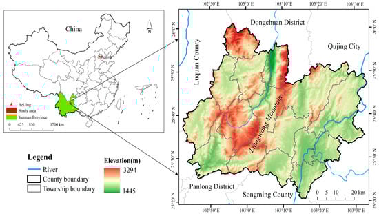
Figure 1. Location of Xundian County in China.

Therefore, Xundian County provides an ideal testing ground for evaluating and improving cropland identification methods under complex topographic and environmental conditions. The objective of this study is to develop and validate a robust cropland identification framework that effectively integrates multispectral, SAR, and topographic data to provide a generalizable and scalable solution for precision agricultural mapping in plateau and mountainous regions.

2.2. Data Sources and Preprocessing

2.2.1. Data Sources

The datasets used in this study and their corresponding sources are summarized as follows:

(1) Remote sensing data: All datasets were obtained from the Google Earth Engine (GEE) platform. Optical data were derived from the COPERNICUS/S2_SR_HARMONIZED surface reflectance (SR) product, while radar data were obtained from the Sentinel-1 C-SAR Ground Range Detected (S1_GRD) product in Interferometric Wide (IW) mode. Both ascending and descending orbit acquisitions were included to enhance temporal coverage and reduce data gaps. All datasets covered the period from January to December 2020, capturing the full cropland phenological cycle—including sowing, growth, and harvest stages.

(2) Topographic data: Topographic variables were derived from the Shuttle Radar Topography Mission (SRTM) DEM dataset, providing elevation and slope information essential for terrain correction and analysis in mountainous regions.

(3) Land use classification products: Three existing land use classification datasets were employed for sample point collection: products from the European Space Agency (ESA), the Environmental Systems Research Institute (ESRI), and the China Resource and Environment Data Cloud (CRLC). These datasets were integrated to ensure broad spatial representativeness and cross-validation of sample accuracy. The details of these datasets are provided in Table 1.

Table 1. Data types and sources.

Data Types	Data Name	Resolution	Year	Data Sources
Sentinel-2	Blue (B2)	10 m	2020	https://developers.google.cn/earth-engine/datasets/catalog/sentinel-2?hl=zh-cn (accessed on 5 July 2025)
	Green (B3)
	Red (B4)
	Red edge 1 (B5)	20 m
	Red edge 2 (B6)
	Red edge 3 (B7)
	Near-Infrared (B8)	10 m
	Narrow Near-Infrared (B8A)	20 m
	Short-Wave Infrared 2 (B11)
	Short-Wave Infrared 3 (B12)
Sentinel-1	VV VH	10 m		Sentinel-1 SAR GRD: C-band Synthetic Aperture Radar Ground Range Detected, log scaling|Earth Engine Data Catalog|Google for Developers
LULC	ESA	10 m		https://developers.google.com/earth-engine/datasets/catalog/ESA_WorldCover_v100 (accessed on 5 July 2025)
	ESRI	10 m		https://www.arcgis.com/home/item.html?id=cfcb7609de5f478eb7666240902d4d3d (accessed on 5 July 2025)
	CRLC	10 m		https://github.com/LiuGalaxy/CRLC?tab=readme-ov-file (accessed on 5 July 2025)
Topographic data	SRTM	30 m	2007	30-Meter SRTM Elevation Data Downloader

2.2.2. Data Preprocessing

Different datasets were processed using appropriate methods tailored to their characteristics:

(1) Sentinel-2 data: To mitigate cloud contamination, the Cloud Score+ algorithm was applied for cloud removal [22]. All 20 m resolution bands were resampled to 10 m for consistency. To capture phenological variation effectively, time-series Sentinel-2 reflectance data were transformed into percentile-based indicators (e.g., 5th, 25th, and 50th percentiles) across the growing season. This approach minimizes the impact of outliers and residual cloud artifacts while preserving key temporal variation patterns related to crop growth.

(2) SAR data: Sentinel-1 Level-1 Ground Range Detected (GRD) data were preprocessed following the European Space Agency (ESA) standard workflow. Steps included orbit correction, thermal noise removal, and radiometric calibration to convert digital numbers into sigma⁰ backscatter coefficients (in decibels). Speckle filtering was conducted using the Lee filter, and terrain correction was applied via the Range–Doppler method using SRTM DEM data to ensure geometric and radiometric normalization across varying terrain. The resulting gamma⁰ products provided radiometrically consistent, terrain-corrected backscatter suitable for integration with optical features in cropland classification [23,24,25].

(3) Slope and aspect data: Slope and aspect layers were derived from the SRTM DEM using the ArcGIS platform (Version 10.8).

(4) Land use/land cover data: To ensure consistency across datasets, the ESA, ESRI, and CRLC land use classification products were reclassified to a unified scheme. Through spatial overlay analysis and visual interpretation, inconsistencies were corrected, and spatially uniform sample points were randomly and evenly distributed across the study area.

(5) Sample points: A total of 4000 sample points were collected, comprising 2000 cropland, 500 forest, 500 grassland, 500 water bodies, and 500 impervious surfaces. Sample selection was based on a spatial overlay of ESA World Cover, ESRI Land Cover, and China Land Cover (CLCD) datasets to ensure broad spatial representation and minimize clustering bias. The Third National Land Survey (TNLS) dataset served as the authoritative benchmark for land use validation, and manual visual interpretation was conducted for partial samples. In addition, 30 cropland parcels were field-verified on 22 July 2025, with local villagers confirming that these plots had remained unchanged for several years. Corresponding field photos are presented in Figure 2. This integrated validation approach—combining random sampling, TNLS-based visual interpretation, and limited field verification—ensured both spatial representativeness and reliable labeling quality. For the classification task, all samples were consolidated into a binary scheme (cropland vs. non-cropland), each containing 2000 samples, ensuring balanced classes and eliminating bias in model training. The spatial distribution of these samples and field photographs is shown in Figure 2.

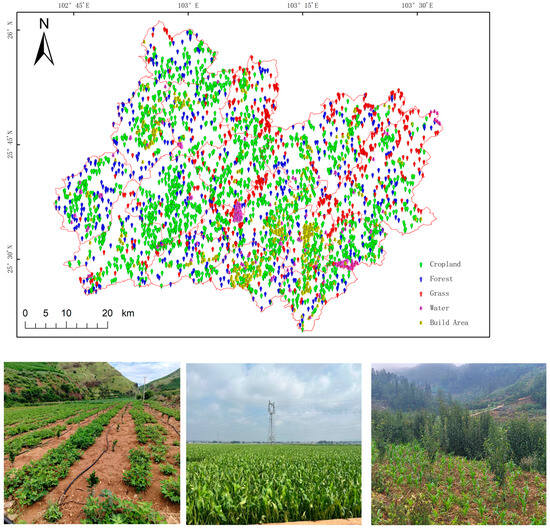
Figure 2. Spatial distribution of training and validation samples derived from overlay analysis, supplemented by field survey verification photographs.

3. Research Methods

3.1. Construction of Feature Dataset

3.1.1. Feature Selection

In addition to the ten spectral bands of Sentinel-2, several commonly used vegetation and water indices were incorporated as classification features, including the Normalized Difference Vegetation Index (NDVI) [26], Enhanced Vegetation Index (EVI) [27], Soil-Adjusted Vegetation Index (SAVI) [28], Normalized Difference Water Index (NDWI), Bare Soil Index (BSI), and Built-up Index (NDBI) [29].

To capture texture characteristics, Grey Level Co-occurrence Matrix (GLCM) metrics were computed from the Sentinel-2 B8 (NIR) band using a 3 × 3 moving window. The GLCM is a widely used statistical texture descriptor in image analysis [30]. Ten texture measures were derived, including Angular Second Moment (ASM), Entropy (ENT), Sum Entropy (SEMT), Difference Entropy (DENT), Sum Average (SAVG), Inverse Difference Moment (IDM), Contrast, Correlation, Difference Variance (SVar), and Variance (Var) [31]. These metrics quantitatively describe surface texture variations, aiding in distinguishing cropland from non-cropland in complex mountainous terrains.

Furthermore, two SAR polarization bands (VV and VH) and polarization-derived indices such as Polarization Ratio (PR), Total Power (TP), Normalized Transformed Polarization Difference (NTPD), and Entropy were included. Finally, topographic variables—including elevation (DEM), slope, and aspect—were added to capture terrain-related spatial heterogeneity.

3.1.2. Temporal Features for Classification

The percentile method implemented in Google Earth Engine (GEE) effectively captures spectral and radar characteristics of Sentinel-2 data and has been widely used in land cover classification. This method constructs histograms for each feature and extracts specified percentile values. For example, using the BLUE (B2) band with percentiles set to 5, 25, 50, 75, and 95 yields five indicators: B2_p5, B2_p25, B2_p50, B2_p75, and B2_p95 [32].

In this study, 5th, 25th, 50th, 75th, and 95th percentiles were selected, resulting in 110 percentile indicators for the ten Sentinel-2 bands, six vegetation/water indices, VV, VH, and four radar indices. This percentile-based approach is particularly suitable for plateau cropland identification, where terrain-driven phenological heterogeneity is pronounced. Unlike fixed-period compositing (e.g., monthly or seasonal averages), the percentile method captures the full reflectance distribution throughout the growing season, preserving phenological extremes (e.g., greening and senescence peaks) while suppressing transient noise such as cloud shadows or illumination differences. This enables the model to effectively distinguish cropland—characterized by strong seasonal cycles—from natural vegetation with relatively stable spectral signatures.

For texture extraction, a 3 × 3 window size was applied when calculating GLCM metrics on 10 m Sentinel-2 imagery. This scale corresponds to the fine spatial structure of plateau cropland, typically composed of small and irregular plots. Larger windows (e.g., 5 × 5 or 7 × 7) tend to oversmooth field boundaries, while smaller ones (e.g., 1 × 1) fail to capture meaningful texture variation. Thus, the 3 × 3 configuration provides an optimal balance between local detail and contextual information, enabling accurate texture characterization under complex terrain conditions.

3.1.3. Feature Selection and Dimensionality Reduction

Given the large and diverse feature space—including 110 percentile-based spectral features, GLCM texture metrics, SAR indices, and topographic variables—a systematic feature selection process was conducted to enhance model robustness and interpretability. Recursive Feature Elimination with Cross-Validation (RFECV) was employed to identify the most informative and non-redundant features. The RFECV procedure used XGBoost as the base estimator, combined with five-fold cross-validation to ensure stability. As shown in Figure 3, the cross-validation accuracy plateaued after approximately 58 features, beyond which additional features did not yield significant gains. Thus, the final optimized subset contained 58 features, balancing model complexity and predictive performance.

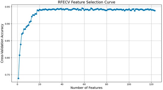
Figure 3. RFECV Feature Selection Curve.

The overall classification workflow is illustrated in Figure 4, consisting of data preprocessing, percentile-based feature extraction, model training with five classifiers, and final cropland identification using the best-performing model.

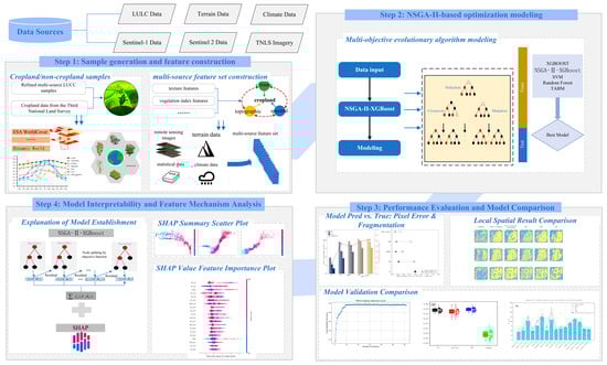
Figure 4. The framework of cropland identification in the study.

3.2. Classifier Construction

To achieve efficient and accurate cropland identification, four widely used and high-performing classifiers were selected: Support Vector Machine (SVM), Random Forest (RF), Extreme Gradient Boosting (XGBoost), and the Tabular Attention-Based Model (TABM). These algorithms were chosen for their proven capability in handling complex, multi-source remote sensing datasets and their strong track records in land cover classification tasks.

Random Forest (RF): An ensemble learning algorithm that constructs multiple decision trees and aggregates their results to enhance stability and accuracy [33].

Support Vector Machine (SVM): A robust supervised learning method particularly suitable for high-dimensional and non-linear data distributions [34].

XGBoost: An efficient implementation of the Gradient Boosted Decision Tree (GBDT) framework, featuring exceptional computational performance and memory efficiency [35]. It supports both L1 (Lasso) and L2 (Ridge) regularization to reduce overfitting and provides built-in feature selection and importance assessment, improving both model interpretability and generalization.

TABM (Tabular Attention-Based Model): As a deep learning baseline, TABM is a Transformer-based architecture specifically designed for structured tabular data [36]. The model employs a multi-head self-attention mechanism to capture complex, non-linear interactions among features. Numerical inputs are transformed using Piecewise-Linear Embeddings, which map continuous variables into 32-dimensional feature vectors across 64 bins, implemented via the rtdl library [37]. This approach integrates state-of-the-art tabular Transformers with advanced feature embeddings, establishing a strong and transparent deep learning baseline for comparison.

The training pipeline was conducted using a 5-fold stratified cross-validation scheme. For each fold, the model was trained for up to 200 epochs using the AdamW optimizer with the following hyperparameters: a learning rate of 1 × 10⁻³, a weight decay of 1 × 10⁻⁵, and a batch size of 128. All input features were preprocessed with a Quantile Transformer. The model state from the epoch yielding the highest kappa on the validation set was saved as the final model for that fold. This entire pipeline establishes TABM as a robust and reproducible deep learning baseline, making it highly suitable for a fair comparison in our cropland identification task.

To further improve the generalization and stability of XGBoost, a Non-dominated Sorting Genetic Algorithm II (NSGA-II) was applied for multi-objective hyperparameter optimization. The optimization simultaneously maximized Overall Accuracy (OA), F1 Score, Recall, and Kappa coefficient, ensuring a balanced trade-off between accuracy and robustness. The optimization was implemented in PyMoo, using a population size of 50 and 80 generations. Each individual represented a unique hyperparameter set, with the following search ranges: learning_rate (0.01–0.3), n_estimators (50–500), and classification threshold (0.01–0.99). Other parameters such as max_depth, lambda, and alpha were fixed based on preliminary grid search results to reduce computational cost. Each candidate solution was evaluated via five-fold cross-validation on the training set. Tournament selection, simulated binary crossover (probability = 0.9), and polynomial mutation (probability = 0.33) were used to preserve diversity and avoid premature convergence. The optimization terminated either after 50 generations or once fitness convergence stabilized.

To ensure reproducibility, the entire optimization process was repeated ten times with different random seeds. The final configuration was selected from the Pareto-optimal front, representing the best compromise between OA and Kappa. All experiments were executed on an RTX GPU (Manufacturer: NVIDIA Corporation, Location: Santa Clara, CA, USA) using the gpu_hist method in XGBoost, with an average runtime of approximately 2.5 h per optimization. Results consistently demonstrated that NSGA-II optimization improved classification stability and reduced performance variance across runs—confirming that performance gains were due to enhanced robustness rather than stochastic variation.

3.3. Accuracy Evaluation Methods

In this study, four evaluation metrics were employed to assess cropland identification performance: Overall Accuracy (OA), Recall, F1 Score, and Kappa Coefficient. OA and Kappa measure the overall accuracy and consistency of classification, while Recall quantifies the model’s ability to correctly identify cropland pixels. The F1 Score integrates both Precision and Recall, offering a balanced evaluation of classification quality. Together, these metrics provide a comprehensive and robust framework for evaluating model performance in cropland identification.

4. Results and Analysis

4.1. Accuracy Analysis of Classification Algorithms

The dataset was randomly divided into ten subsets, with seven used for training and three for validation. Five models—Random Forest (RF), Support Vector Machine (SVM), TABM, XGBoost, and NSGA-II-optimized XGBoost (NSGA-II-XGBoost)—were employed for cropland classification (Table 2). All models achieved strong recognition performance, with OA values exceeding 94%, confirming their effectiveness in this task.

Table 2. Comparison of Classifier Accuracy.

Classifier	OA%	kappa	F1	Recall
RF	94.33	0.88	0.94	0.94
SVM	94.33	0.88	0.94	0.92
TABM	94.88	0.90	0.95	0.95
XGBoost	95.50	0.90	0.95	0.96
NSGA-II-XGBoost	95.75	0.91	0.96	0.96

Classifier comparison: The classification accuracies of RF and SVM were similar, both achieving Recall and F1 Scores above 90%, indicating solid and stable performance. XGBoost outperformed both models across all evaluation metrics, reaching an OA of 95.5%, reflecting its superior capability in capturing non-linear feature interactions.

Spatial distribution analysis: Cropland identification was performed for the entire study area using both XGBoost and NSGA-II-XGBoost models (Figure 5a,b) and compared with cropland distribution from the Third National Land Survey (TNLS) (Figure 5c). Cropland in Xundian County exhibited a fragmented spatial pattern, primarily distributed across river valleys, basins, and low hills. These regions are characterized by relatively flat terrain, fertile soils, and sufficient water resources, making them particularly suitable for agricultural production.

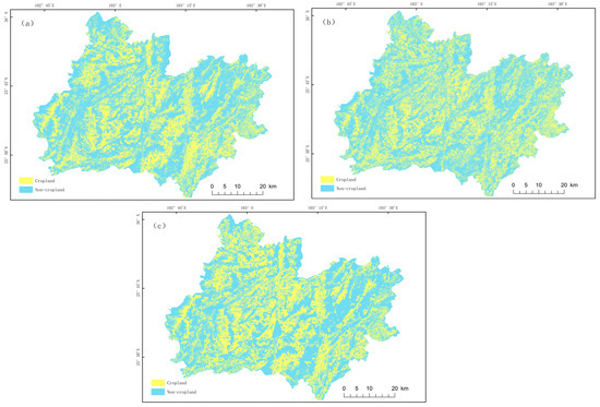
Figure 5. NSGA-II-XGBoost cropland distribution map (a), XGBoost cropland distribution map (b), and cropland distribution map of the Third National Land Survey (c).

Improvement from NSGA-II optimization: Optimization of XGBoost using NSGA-II and five-fold cross-validation yielded consistent improvements in all metrics (Figure 6). The optimized model achieved OA = 95.75%, Kappa = 0.91, and Recall and F1 = 0.96. Although the numerical increase in OA (ΔOA = +0.25%) appears small, spatial analysis revealed noticeable enhancements in classification quality. The NSGA-II-XGBoost results exhibited smoother and more continuous cropland patches, reduced over-fragmentation, and improved boundary integrity—particularly in mountainous and basin transition zones. This indicates that the NSGA-II optimization strengthened the model’s spatial coherence and boundary delineation capability, not just pixel-level accuracy. As shown in Figure 5 and Figure 7, cropland boundaries extracted by NSGA-II-XGBoost aligned more closely with TNLS reference data, effectively capturing fragmented cropland in valley regions and minimizing confusion between cropland and grassland. Thus, even a minor numerical improvement in OA translated into a substantial spatial enhancement, which holds greater practical significance for high-precision mapping and land management in complex plateau environments.

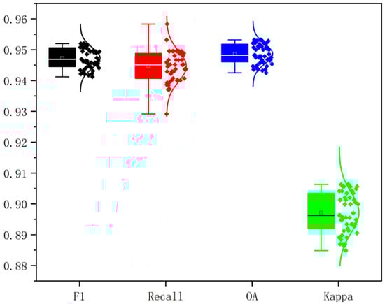
Figure 6. Results of the 5-fold cross-validation for the indicator.

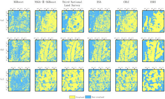
Figure 7. Comparison of three typical cropland plots.

However, accuracy derived from random splits may exhibit optimistic bias due to spatial autocorrelation. Neighboring pixels often share similar spectral or textural characteristics, causing training and validation samples to be spatially dependent—leading to artificially inflated accuracy scores.

Additionally, the TNLS dataset reveals a pronounced class imbalance (cropland accounts for only ~34% of the total area), presenting greater challenges than the balanced training samples typically used. To mitigate these biases, we conducted an independent validation using the official TNLS raster dataset as an external, wall-to-wall ground truth for pixel-level evaluation. This approach provides an unbiased and spatially independent benchmark for model performance assessment.

To ensure comparability with state-of-the-art approaches, we included a Tabular Attention-Based Model (TABM) as a deep learning baseline (Table 3). Given that our workflow is based on pixel-level tabular features rather than image patches, TABM provides a more appropriate deep learning alternative than conventional semantic segmentation networks.

Table 3. Pixel-wise Accuracy Validation with TNLS Reference Data.

Model	OA	Precision	Recall	F1	IoU	BIoU
RF	0.7424	0.7265	0.4064	0.5271	0.3446	0.2729
SVM	0.7577	0.7603	0.4167	0.5383	0.3683	0.2867
XGBoost	0.774	0.6494	0.7249	0.6851	0.521	0.2738
TABM	0.828	0.7171	0.8137	0.7624	0.616	0.2974
NSGA-II-XGBoost	0.8325	0.7321	0.798	0.7637	0.6177	0.3049

In addition to traditional metrics, Intersection over Union (IoU) and Boundary IoU were introduced to quantify boundary delineation performance. Under this rigorous independent validation, the NSGA-II-XGBoost model achieved the highest overall accuracy (OA = 0.8325, F1 = 0.7637, IoU = 0.6177), while its Boundary IoU (0.3049) exceeded all other models, including TABM. This result demonstrates the model’s superior capability in detecting fragmented cropland boundaries under complex topographic conditions.

In summary, the NSGA-II-XGBoost model achieved both stable accuracy improvements and significantly enhanced spatial recognition performance. These findings highlight its suitability for cropland identification in complex terrain, providing a reliable and generalizable approach for high-precision land use classification.

In this study, cropland recognition results from XGBoost and NSGA-II-XGBoost models were further compared with the actual cropland distribution derived from the Third National Land Survey. To more thoroughly assess performance, three representative cropland regions with substantial spatial differences were selected for detailed analysis. These regions encompass diverse land use types and topographic conditions, all located above 1900 m elevation with slopes exceeding 25°, representing typical high-altitude cropland areas.

In this study, cropland recognition results from XGBoost and NSGA-II-XGBoost models were further compared with the actual cropland distribution derived from the Third National Land Survey.

To more thoroughly assess performance, three representative cropland regions with substantial spatial differences were selected for detailed analysis (Figure 7). These regions encompass diverse land use types and topographic conditions, all located above 1900 m elevation with slopes exceeding 25°, representing typical high-altitude cropland areas.

As shown in Table 4, the NSGA-II-XGBoost model achieved SPLIT (3.2952) and SHDI (0.6589) values that were closest to those of the reference dataset (SPLIT = 2.5119; SHDI = 0.6404). In contrast, models such as RF (4.6595) and TABM (4.2615) exhibited substantially higher SPLIT values, indicating excessive “salt-and-pepper” noise and more fragmented patch structures in their classification outputs. These quantitative landscape and boundary metrics provide robust evidence that the optimized model proposed in this study offers clear advantages in maintaining cropland spatial continuity and suppressing fragmentation, with a resulting spatial pattern most consistent with actual land surface conditions.

Table 4. Landscape Pattern Index Comparison.

Model	SPLIT	SHDI
Ground Truth	2.5119	0.6404
NSGA-II-XGBoost	3.2952	0.6589
XGBoost	3.5034	0.6636
TABM	4.2615	0.6665
SVM	4.5612	0.6803
RF	4.6595	0.7793

The improvement can be attributed primarily to the multi-objective optimization framework of NSGA-II-XGBoost, which simultaneously refined hyperparameter settings and feature combinations, thereby enhancing the model’s adaptability to complex data relationships. This advantage was particularly evident in regions where cropland–non-cropland boundaries were ambiguous or spectral characteristics overlapped.

A notable strength of the NSGA-II-XGBoost model lies in its capacity to effectively integrate spectral and topographic features (e.g., NDVI, EVI, VH, VV, slope, and elevation). These features are crucial for discriminating cropland from other land cover types, especially in heterogeneous mountainous terrain. Through multi-objective optimization, the model automatically selected the most informative feature subset, effectively reducing overfitting while enhancing accuracy and generalization. When compared with the Third National Land Survey reference data, NSGA-II-XGBoost not only produced more spatially coherent predictions but also better preserved the intrinsic heterogeneity of cropland boundaries.

In particular, the model demonstrated strong potential for large-scale cropland monitoring in complex landscapes—not due to dramatic numerical accuracy gains, but because of its enhanced reliability, stability, and interpretability.

Its significant advantages in accurately delineating cropland boundaries and identifying land use transitions underscore its promise for high-precision cropland mapping and land resource management applications.

4.2. Feature Analysis

4.2.1. Overall Analysis

An in-depth analysis of cropland features was conducted using the XGBoost–SHAP model. Results revealed that the five most influential features contributing to cropland recognition accuracy in Xundian County were B4_p5, VH_p5, slope, EVI_p5, and B2_p5.

These variables demonstrated the strongest contributions to classification performance, confirming that spectral, topographic, and vegetation-related features play a dominant role in distinguishing cropland from non-cropland in complex plateau environments.

The SHAP value distribution and feature heatmap analysis (Figure 8) further showed that p5-type percentile features and topographic attributes ranked highest in importance. This finding suggests that, compared with other percentile-based indicators, p5-level features capture the most discriminative phenological and reflectance characteristics in high-altitude, mountainous conditions.

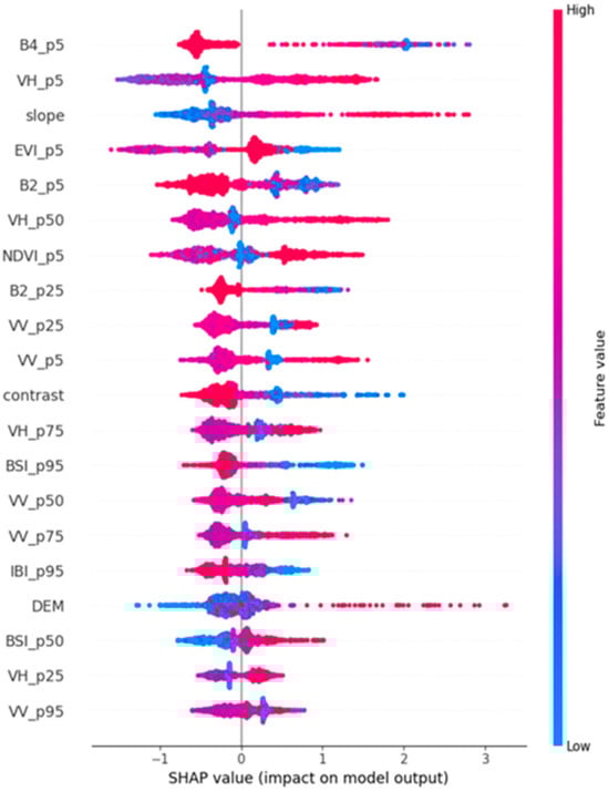
Figure 8. Visualization of SHAP values for the first 20 features.

In these environments, integrating spectral and topographic information is essential for improving model robustness and classification precision.

4.2.2. Feature Dependence Analysis

Based on SHAP importance rankings, the top five key features were selected to analyze their detailed effects on cropland identification. Corresponding SHAP dependence plots are shown in Figure 9, and their interpretations are summarized below:

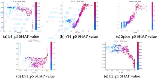
Figure 9. SHAP dependency graph for the first five features.

B4_p5: When reflectance values fall within 0–0.2, B4 values are generally low—typically corresponding to dense vegetation or water bodies, both of which contribute positively and stably to model predictions. As reflectance increases toward ~0.25, it may represent sparse vegetation or bare soil, introducing classification uncertainty and reducing SHAP values. Higher reflectance values (>0.25) often indicate mixed surfaces (e.g., soil–vegetation mixtures), which increase confusion and decrease classification confidence.

VH_p5: SHAP values are negative within –30 to –24 dB, suggesting that this range represents bare or sparsely vegetated surfaces, inconsistent with cropland. Between –24 and –15 dB, SHAP values become positive, indicating stronger associations with moist or partially vegetated cropland surfaces—thus contributing positively to model accuracy.

Slope: SHAP values increase with slope, implying that moderate slopes contribute positively to cropland identification. While flat terrain may seem favorable for cultivation, its spectral similarity to built-up or water-covered areas reduces discriminative power. In contrast, moderate-slope areas, such as terraced farmland, align well with the typical cropland morphology in the study area, yielding the strongest positive contribution.

EVI_p5: Both low and high EVI values contribute positively, while intermediate values exert a negative effect. Low EVI values correspond to sparse vegetation or bare soil, which are easily classified; high EVI values indicate dense vegetation, also distinctive. Intermediate EVI ranges often represent transitional vegetation states (e.g., mixed cropland and grassland), increasing classification ambiguity and lowering SHAP scores.

B2_p5: SHAP values decrease as B2 reflectance increases. When B2 exceeds approximately 0.2, its contribution turns negative. Low B2 values, often corresponding to water bodies, provide strong and consistent signals, enhancing classification accuracy. Conversely, high B2 values are linked to bare land or urban areas, introducing spectral confusion and reducing model reliability.

5. Discussion

5.1. Comparison with the Third National Land Survey Data

The cropland distribution identified by the NSGA-II–XGBoost model in Xundian County was generally consistent with the Third National Land Survey (TNLS) data, with only minor discrepancies observed in Jinsuo, Kedu, Qixing, and Hekou towns (Figure 10). These differences primarily occurred in complex mountainous areas characterized by steep slopes and dense vegetation, where the model tended to misclassify cropland as natural vegetation. Similar challenges have been widely reported in mountainous land cover studies, where topographic heterogeneity, illumination effects, and mixed spectral responses reduce classification accuracy [38,39]. The misclassification sources identified in this study—terrain complexity, vegetation density, spectral overlap, and boundary ambiguity—are consistent with prior findings. In mountainous and urban areas, the high heterogeneity of vegetation growth and cultivation patterns leads to severe spectral and backscatter signal mixing. Moreover, frequent cloud cover and rainfall events often result in missing observations in optical imagery and unexpected noise in SAR time-series data, ultimately reducing data availability and quality in cloud-prone regions. These factors jointly increase classification uncertainty and complicate precise cropland identification in complex terrains [40,41].

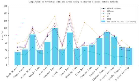
Figure 10. Comparison of township-level cropland area.

In addition, the relatively close agreement between the model-derived cropland area and TNLS data demonstrates that the proposed approach is not only effective in discriminating cropland but also capable of preserving the spatial integrity of agricultural landscapes. This level of spatial consistency suggests that the integration of multisource data—especially the combination of SAR and topographic features—can substantially mitigate terrain-induced distortions. Furthermore, this outcome provides empirical support for using hybrid optical–SAR–topographic models in regions where conventional optical-only methods often fail due to persistent cloud coverage or illumination effects.

5.2. Comparative Performance and Model Advantages

Compared with conventional classifiers such as RF, SVM, TABM, and standard XGBoost, the NSGA-II–XGBoost model demonstrated superior accuracy, stability, and adaptability. Its multi-objective optimization framework simultaneously tunes hyperparameters and decision thresholds, effectively balancing accuracy and generalization. This aligns with previous studies where evolutionary optimization has been successfully integrated with machine learning for remote sensing classification [42].

The model’s optimization strategy enables efficient exploration of complex parameter spaces, overcoming the manual tuning limitations seen in traditional algorithms. The use of NSGA-II provides a global search mechanism that mitigates overfitting and enhances performance across varying terrain and climatic conditions. The ability to integrate optical, SAR, and topographic features further strengthens the model’s robustness in capturing both spectral and structural land surface information. In particular, the improvement in spatial coherence and the suppression of “salt-and-pepper” noise observed in this study indicate that the NSGA-II–XGBoost model achieves a more realistic depiction of cropland distribution patterns, especially in fragmented agricultural mosaics. Nevertheless, certain challenges persist. First, since the algorithm involves population-based iterative optimization, the computational cost of the model remains relatively high, consistent with previous findings that parallel computing or GPU acceleration can substantially improve computational efficiency [43]. Second, the NSGA-II algorithm exhibits sensitivity to parameter settings, requiring careful initialization to avoid premature convergence [44]. Third, the trade-off between classification accuracy and computational efficiency has not yet been fully resolved; future research could explore adaptive weighting strategies or multi-fidelity optimization approaches to address this limitation [45].

Overall, the model’s robustness across complex terrain demonstrates the promise of multi-objective evolutionary optimization for remote sensing–based land classification tasks, particularly when integrating heterogeneous data sources such as optical, SAR, and topographic variables. Furthermore, these findings reinforce the growing view that hybrid learning models—combining physics-based and data-driven principles—represent a critical direction for high-precision agricultural mapping in complex landscapes. The integration of evolutionary optimization into existing classification pipelines also provides a practical pathway for improving traditional algorithms without requiring large-scale model redesign.

5.3. Applicability and Generalization Analysis

To test the transferability of the NSGA-II–XGBoost model, an independent validation was conducted in Binchuan County, Yunnan Province. Despite differences in topography and climate, the model achieved an OA of 98.50%, Kappa of 0.97, F1 score of 0.9848, and Recall of 0.9783, indicating high robustness and reproducibility. This finding aligns with recent studies showing that hybrid optical–SAR approaches can achieve strong cross-regional generalization when appropriate temporal and topographic features are integrated [46]. The generalization performance across different regions suggests that the proposed framework can effectively adapt to varying environmental conditions and vegetation phenologies, maintaining reliable discrimination between cropland and non-cropland areas. However, the dependence on percentile-based temporal metrics may reduce model accuracy where time-series continuity is disrupted. Incorporating multi-sensor temporal fusion or deep temporal networks could alleviate these issues in future applications [47]. Moreover, the results from Binchuan indicate that the model’s feature selection and optimization strategies can be successfully transferred with minimal adjustment, supporting its scalability for operational use. This highlights its potential for integration into automated national land-monitoring frameworks, where models must adapt to diverse eco-climatic gradients with limited manual calibration. Beyond cropland mapping, the same optimization strategy could be extended to other land cover applications—such as forest degradation monitoring or wetland change detection—further underscoring its flexibility and cross-domain value.

Additionally, the reproducibility achieved across two ecologically distinct regions implies that the proposed approach has the capacity to capture universal relationships between vegetation, terrain, and spectral properties. This makes it particularly suitable for long-term agricultural and environmental monitoring under changing climate conditions, where temporal consistency and spatial adaptability are crucial.

5.4. Limitations and Future Perspectives

While the NSGA-II–XGBoost model achieved high accuracy, several limitations should be addressed to further improve its generalization and operational applicability.

First, the 30 m SRTM DEM may not sufficiently capture fine-scale topographic variations in mountainous regions. Studies utilizing higher-resolution elevation data, such as ALOS (12.5 m) or LiDAR (5 m), have shown notable improvements in cropland classification within terraced landscapes [48].

Second, the current framework could be extended toward a spatio-temporal adaptive optimization system, in which the genetic algorithm dynamically adjusts parameters across different terrain zones and seasons. Such a regionally adaptive scheme would enhance transferability and reduce the need for manual calibration in heterogeneous environments [49].

Third, future studies should explore explainable and uncertainty-aware machine learning frameworks, enabling the quantification of model confidence and the identification of error sources related to terrain, vegetation, or sensor noise. This would provide stronger interpretability and facilitate integration with decision-support systems for precision agriculture and land management [50].

In addition, coupling the proposed model with cloud-based geospatial processing platforms (e.g., Google Earth Engine or ESA Data Cube) could enable large-scale, near-real-time cropland monitoring. This integration would allow continuous updates to agricultural maps and support dynamic decision-making for land use management. Furthermore, as open-access satellite constellations continue to expand, incorporating hyperspectral or radar polarimetric data could significantly enhance the detection of subtle variations in vegetation structure and soil moisture, further improving classification accuracy.

Future research should therefore focus on:

(1)

Integrating high-resolution topographic and spectral data to enhance detection of small terraces and steep-slope cropland.

(2)

Developing spatio-temporal adaptive optimization frameworks that enable automatic parameter adjustment across heterogeneous landscapes.

(3)

Incorporating explainable and uncertainty-aware AI approaches to improve model transparency and support operational decision-making.

By incorporating these strategies, the NSGA-II–XGBoost framework can evolve into a powerful, adaptive, and interpretable tool for fine-scale agricultural monitoring, supporting evidence-based land use management and sustainable development in complex mountainous regions.

6. Conclusions

This study proposed an optimized NSGA-II–XGBoost framework to address the challenge of cropland identification in complex plateau and mountainous regions by integrating multi-source datasets—including spectral, radar, and topographic features—with an improved sample selection strategy. The main conclusions are as follows:

(1)

Model performance: The NSGA-II–XGBoost model significantly improved classification accuracy and generalization through multi-objective optimization of hyperparameters and feature combinations. Compared with RF, SVM, TABM and standard XGBoost, it achieved superior accuracy, computational efficiency, and robustness, particularly in identifying cropland with complex boundaries or spectral similarity.

(2)

Feature contributions: Feature importance analysis showed that spectral, radar, and topographic variables all contributed substantially to cropland recognition. Terrain factors such as slope and elevation were especially influential in plateau and hilly regions. Percentile-based features (e.g., VH_p5) effectively captured detailed feature distributions, improving classification reliability.

(3)

Sample strategy: The integration of multiple land cover products and uniform random sampling enhanced the balance and representativeness of training data, leading to improved model performance.

Overall, the proposed NSGA-II–XGBoost framework provides an efficient, accurate, and generalizable approach for cropland mapping in complex terrain, offering strong potential for broader applications in precision land use classification, cropland monitoring, and sustainable resource management.

References

- Shi, S.; Han, Y.; Yu, W.; Cao, Y.; Cai, W.; Yang, P.; Wu, W.; Yu, Q. Spatio-temporal differences and factors influencing intensivecropland use in the Huang-Huai-Hai Plain. J. Geogr. Sci. 2018, 28, 1626–1640. [Google Scholar] [CrossRef]
- Wang, J.; Lin, Y.; Glendinning, A.; Xu, Y. Land-use changes and land policies evolution in China’s urbanization processes. Land Use Policy 2018, 75, 375–387. [Google Scholar] [CrossRef]
- Liu, Y.; Zhou, Y. Reflections on China’s food security and land use policy under rapid urbanization. Land Use Policy 2021, 109, 105699. [Google Scholar] [CrossRef]
- Liu, F.; Zhang, Z.; Zhao, X.; Wang, X.; Zuo, L.; Wen, Q.; Yi, L.; Xu, J.; Hu, S.; Liu, B. Chinese cropland losses due to urban expansion in the past four decades. Sci. Total. Environ. 2019, 650, 847–857. [Google Scholar] [CrossRef]
- Chen, G.; Zhao, J.; Duan, X.; Tang, B.; Zuo, L.; Wang, X.; Guo, Q. Spatial Quantification of Cropland Soil Erosion Dynamics in the Yunnan Plateau Based on Sampling Survey and Multi-Source LUCC Data. Remote Sens. 2024, 16, 977. [Google Scholar] [CrossRef]
- Xue, S.; Fang, Z.; van Riper, C.; He, W.; Li, X.; Zhang, F.; Wang, T.; Cheng, C.; Zhou, Q.; Huang, Z.; et al. Ensuring China’s food security in a geographical shift of its grain production: Driving factors, threats, and solutions. Resour. Conserv. Recycl. 2024, 210, 107845. [Google Scholar]
- Chen, Z.; Shi, D. Spatial structure characteristics of slope farmland quality in Plateau mountain area: A case study of Yunnan Province, China. Sustainability 2020, 12, 7230. [Google Scholar] [CrossRef]
- Ye, S.; Ren, S.; Song, C.; Du, Z.; Wang, K.; Du, B.; Cheng, F.; Zhu, D. Spatial pattern of cultivated land fragmentation in mainland China: Characteristics, dominant factors, and countermeasures. Land Use Policy 2024, 139, 107070. [Google Scholar] [CrossRef]
- Zhao, S.; Yin, M. Change of urban and rural construction land and driving factors of arable land occupation. PLoS ONE 2023, 18, e0286248. [Google Scholar]
- Sumbo, D.K.; Anane, G.K.; Inkoom, D.K.B. ‘Peri-urbanisation and loss of arable land’: Indigenes’ farmland access challenges and adaptation strategies in Kumasi and Wa, Ghana. Land Use Policy 2023, 126, 106534. [Google Scholar] [CrossRef]
- Lü, G.; Batty, M.; Strobl, J.; Lin, H.; Zhu, A.X.; Chen, M. Reflections and speculations on the progress in Geographic Information Systems (GIS): A geographic perspective. Int. J. Geogr. Inf. Sci. 2019, 33, 346–367. [Google Scholar] [CrossRef]
- Pandey, P.C.; Pandey, M. Highlighting the role of agriculture and geospatial technology in food security and sustainable development goals. Sustain. Dev. 2023, 31, 3175–3195. [Google Scholar] [CrossRef]
- Shen, Q.; Deng, H.; Wen, X.; Chen, Z.; Xu, H. Statistical texture learning method for monitoring abandoned suburban cropland based on high-resolution remote sensing and deep learning. IEEE J. Sel. Top. Appl. Earth Obs. Remote Sens. 2023, 16, 3060–3069. [Google Scholar] [CrossRef]
- Abdi, A.M. Land cover and land use classification performance of machine learning algorithms in a boreal landscape using Sentinel-2 data. GISci. Remote Sens. 2020, 57, 1–20. [Google Scholar] [CrossRef]
- Shao, Z.; Ahmad, M.N.; Javed, A. Comparison of random forest and XGBoost classifiers using integrated optical and SAR features for map** urban impervious surface. Remote Sens. 2024, 16, 665. [Google Scholar] [CrossRef]
- Wang, N.; Naz, I.; Aslam, R.W.; Quddoos, A.; Soufan, W.; Raza, D.; Ishaq, T.; Ahmed, B. Spatio-Temporal Dynamics of Rangeland Transformation using machine learning algorithms and Remote Sensing data. Rangel. Ecol. Manag. 2024, 94, 106–118. [Google Scholar] [CrossRef]
- Yi, Z.; Jia, L.; Chen, Q.; Jiang, M.; Zhou, D.; Zeng, Y. Early-season crop identification in the Shiyang River Basin using a deep learning algorithm and time-series Sentinel-2 data. Remote Sens. 2022, 14, 5625. [Google Scholar] [CrossRef]
- Wang, X.; Fang, S.; Yang, Y.; Du, J.; Wu, H. A New Method for Crop Type Mapping at the Regional Scale Using Multi-Source and Multi-Temporal Sentinel Imagery. Remote Sens. 2023, 15, 2466. [Google Scholar] [CrossRef]
- Liu, Q.; Wu, Z.; Cui, N.; Jin, X.; Zhu, S.; Jiang, S.; Zhao, L.; Gong, D. Estimation of soil moisture using multi-source remote sensing and machine learning algorithms in farming land of Northern China. Remote Sens. 2023, 15, 4214. [Google Scholar] [CrossRef]
- Hao, Q.; Zhang, T.; Cheng, X.; He, P.; Zhu, X.; Chen, Y. GIS-based non-grain cultivated land susceptibility prediction using data mining methods. Sci. Rep. 2024, 14, 4433. [Google Scholar] [CrossRef]
- Sun, X.; Zhou, C.; Xie, J.; Ouyang, Z.; Luo, Y. SRTM DEM correction based on PSO-DBN model in vegetated mountain areas. Forests 2023, 14, 1985. [Google Scholar] [CrossRef]
- Liang, K.; Yang, G.; Zuo, Y.; Chen, J.; Sun, W.; Meng, X.; Chen, B. A Novel Method for Cloud and Cloud Shadow Detection Based on the Maximum and Minimum Values of Sentinel-2 Time Series Images. Remote Sens. 2024, 16, 1392. [Google Scholar]
- Vollrath, A.; Mullissa, A.; Reiche, J. Angular-based radiometric slope correction for Sentinel-1 on google earth engine. Remote Sens. 2020, 12, 1867. [Google Scholar] [CrossRef]
- Choi, H.; Jeong, J. Speckle noise reduction technique for SAR images using statistical characteristics of speckle noise and discrete wavelet transform. Remote Sens. 2019, 11, 1184. [Google Scholar] [CrossRef]
- Shi, C.; Zuo, X.; Zhang, J.; Zhu, D.; Li, Y.; Bu, J. Accuracy Assessment of Geometric-Distortion Identification Methods for Sentinel-1 Synthetic Aperture Radar Imagery in Highland Mountainous Regions. Sensors 2024, 24, 2834. [Google Scholar] [CrossRef] [PubMed]
- Tucker, C.J. Red and photographic infrared linear combinations for monitoring vegetation. Remote Sens. Environ. 1979, 8, 127–150. [Google Scholar] [CrossRef]
- Huete, A.; Didan, K.; Miura, T.; Rodriguez, E.P.; Gao, X.; Ferreira, L.G. Overview of the radiometric and biophysical performance of the MODIS vegetation indices. Remote Sens. Environ. 2002, 83, 195–213. [Google Scholar] [CrossRef]
- Huete, A.R. A soil adjusted vegetation index (SAVI). Remote Sens. Environ. 1988, 25, 295–309. [Google Scholar] [CrossRef]
- Kulkarni, K.; Vijaya, P.A. NDBI based prediction of land use land cover change. J. Indian Soc. Remote Sens. 2021, 49, 2523–2537. [Google Scholar]
- Tavus, B.; Kocaman, S.; Gokceoglu, C. Flood damage assessment with Sentinel-1 and Sentinel-2 data after Sardoba dam break with GLCM features and Random Forest method. Sci. Total. Environ. 2022, 816, 151585. [Google Scholar] [CrossRef]
- Wang, S.; Feng, W.; Quan, Y.; Li, Q.; Dauphin, G.; Huang, W.; Li, J.; Xing, M. A heterogeneous double ensemble algorithm for soybean planting area extraction in Google Earth Engine. Comput. Electron. Agric. 2022, 197, 106955. [Google Scholar] [CrossRef]
- Zeng, H.; Wu, B.; Wang, S.; Musakwa, W.; Tian, F.; Mashimbye, Z.E.; Poona, N.; Syndey, M. A synthesizing land-cover classification method based on Google Earth engine: A case study in Nzhelele and Levhuvu Catchments, South Africa. Chin. Geogr. Sci. 2020, 30, 397–409. [Google Scholar] [CrossRef]
- Dou, J.; Yunus, A.P.; Bui, D.T.; Merghadi, A.; Sahana, M.; Zhu, Z.; Chen, C.-W.; Khosravi, K.; Yang, Y.; Pham, B.T. Assessment of advanced random forest and decision tree algorithms for modeling rainfall-induced landslide susceptibility in the Izu-Oshima Volcanic Island, Japan. Sci. Total. Environ. 2019, 662, 332–346. [Google Scholar] [CrossRef] [PubMed]
- Peng, C.; Cheng, J.; Cheng, Q. A supervised learning model for high-dimensional and large-scale data. ACM Trans. Intell. Syst. Technol. 2016, 8, 1–23. [Google Scholar] [CrossRef]
- Tang, S. The box office prediction model based on the optimized XGBoost algorithm in the context of film marketing and distribution. PLoS ONE 2024, 19, e0309227. [Google Scholar] [CrossRef]
- Gorishniy, Y.; Kotelnikov, A.; Babenko, A. Tabm: Advancing tabular deep learning with parameter-efficient ensembling. arXiv 2024, arXiv:2410.24210. [Google Scholar]
- Gorishniy, Y.; Rubachev, I.; Khrulkov, V.; Babenko, A. Revisiting deep learning models for tabular data. Adv. Neural Inf. Process. Syst. 2021, 34, 18932–18943. [Google Scholar]
- Huang, D.; Zhou, Z.; Zhang, Z.; Dai, Q.; Lu, H.; Li, Y.; Huang, Y. Land Use/Land Cover Remote Sensing Classification in Complex Subtropical Karst Environments: Challenges, Methodological Review, and Research Frontiers. Appl. Sci. 2025, 15, 9641. [Google Scholar] [CrossRef]
- Gao, L.; Luo, J.; Xia, L.; Wu, T.; Sun, Y.; Liu, H. Topographic constrained land cover classification in mountain areas using fully convolutional network. Int. J. Remote Sens. 2019, 40, 7127–7152. [Google Scholar] [CrossRef]
- Xu, S. Employing Optical and SAR Imagery for Enhanced Mapping of Vegetation and Crops in Challenging Environments. Ph.D. Thesis, The Hong Kong Polytechnic University, Hong Kong, China, 2024. [Google Scholar]
- Li, Y.; Zhao, R.; Wang, Y. Mapping Ratoon Rice Fields Based on SAR Time Series and Phenology Data in Cloudy Regions. Remote Sens. 2024, 16, 2703. [Google Scholar] [CrossRef]
- Ma, A.; Wan, Y.; Zhong, Y.; Wang, J.; Zhang, L. SceneNet: Remote sensing scene classification deep learning network using multi-objective neural evolution architecture search. ISPRS J. Photogramm. Remote Sens. 2021, 172, 171–188. [Google Scholar]
- Liu, Z.; Xu, X.; Qiao, P.; Li, D. Acceleration for deep reinforcement learning using parallel and distributed computing: A survey. ACM Comput. Surv. 2024, 57, 1–35. [Google Scholar] [CrossRef]
- Verma, S.; Pant, M.; Snasel, V. A comprehensive review on NSGA-II for multi-objective combinatorial optimization problems. IEEE Access 2021, 9, 57757–57791. [Google Scholar]
- Zhang, R.; Alemazkoor, N. Multi-fidelity machine learning for uncertainty quantification and optimization. J. Mach. Learn. Model. Comput. 2024, 5, 77–94. [Google Scholar] [CrossRef]
- Wang, N.; Guan, Y.; Wang, Y.; Fang, Q.; Li, Z.; Dong, J.; Luo, J. Automated Extraction of Impervious Surface Area Using Hyper–Local Samples from Multi-Source Data Fusion Across Economic–Geographic Zones. IEEE J. Sel. Top. Appl. Earth Obs. Remote Sens. 2025, 18, 22602–22619. [Google Scholar]
- Qiao, H.; Wang, T.; Wang, P.; Qiao, S.; Zhang, L. A time-distributed spatiotemporal feature learning method for machine health monitoring with multi-sensor time series. Sensors 2018, 18, 2932. [Google Scholar] [CrossRef] [PubMed]
- Jiang, H.; Ku, M.; Zhou, X.; Zheng, Q.; Liu, Y.; Xu, J.; Li, D.; Wang, C.; Wei, J.; Zhang, J.; et al. CropLayer: A high-accuracy 2-meter resolution cropland mapping dataset for China in 2020 derived from Mapbox and Google satellite imagery using data-driven approaches. Earth Syst. Sci. Data Discuss. 2025, 17, 6703–6729. [Google Scholar]
- Fan, Q.; Jiang, M.; Huang, W.; Jiang, Q. Considering spatiotemporal evolutionary information in dynamic multi-objective optimisation. CAAI Trans. Intell. Technol. 2023, 140, 109741. [Google Scholar]
- Tomsett, R.; Preece, A.; Braines, D.; Cerutti, F.; Chakraborty, S.; Srivastava, M.; Pearson, G.; Kaplan, L. Rapid trust calibration through interpretable and uncertainty-aware AI. Patterns 2020, 1, 100049. [Google Scholar] [CrossRef]
Disclaimer/Publisher’s Note: The statements, opinions and data contained in all publications are solely those of the individual author(s) and contributor(s) and not of MDPI and/or the editor(s). MDPI and/or the editor(s) disclaim responsibility for any injury to people or property resulting from any ideas, methods, instructions or products referred to in the content. |
© 2025 by the authors. Licensee MDPI, Basel, Switzerland. This article is an open access article distributed under the terms and conditions of the Creative Commons Attribution (CC BY) license.