Aerodynamic Roughness Retrieval at Typical Antarctic Stations Based on Multi-Source Remote Sensing

Highlights

What are the main findings?

• A Raupach-based framework successfully retrieved aerodynamic roughness using UAV, REMA, and ICESat-2 data.
• The aerodynamic roughness (z_0m) derived from ICESat-2 ATL06 data demonstrated accuracy comparable to that from the ATL03 data, with optimal performance achieved at a 2 km window.

What are the implications of the main findings?

• This study confirms that the more accessible standard ICESat-2 ATL06 data product can be used for large-scale, high-precision aerodynamic roughness mapping, reducing data processing complexity.
• The finding that elevation changes and slope gradients are the primary factors influencing roughness variability provides key insights for improving parameterizations in climate models and studying land–atmosphere interactions.

Abstract

Antarctica’s aerodynamic roughness length (z_0m) is crucial for surface energy exchange and atmospheric modeling, but its remote sensing estimation remains challenging due to complex ice-surface conditions and limited observations. To address these challenges, this study establishes a z_0m retrieval framework derived from the Raupach model using Unmanned Aerial Vehicle (UAV), Reference Elevation Model of Antarctica (REMA), and Ice, Cloud, and land Elevation Satellite-2 (ICESat-2) datasets at three representative Antarctic sites. The results show that UAV benchmarks yield mean z_0m values of 0.009795, 0.011597, and 0.005203 m at Zhongshan Station, Great Wall Station, and Qinling Station, respectively. In experiments with ICESat-2 data, z_0m derived from ATL06 demonstrates accuracy comparable to that from ATL03 (RMSE = 7.45 × 10⁻⁶ m), with the best performance obtained at a 2 km window. Spatially, the agreement with UAV-derived z_0m decreases in the order: REMA > ICESat-2 (IDW-interpolated). The accuracy of REMA and ICESat-2 decreased with terrain complexity, from ice-free zones to the ice-shelf front and finally to the steep ice sheet margin. The elevation and slope variations emerge as dominant controls of z_0m spatial patterns. This study demonstrates the complementary strengths of UAV, REMA, and ICESat-2 datasets in Antarctic aerodynamic roughness estimation, providing practical guidance for data selection and methodology optimization. This study develops an improved z_0m retrieval method for Antarctica, clarifies the applicability and limitations of UAV, REMA, and ICESat-2 data, and provides methodological and data support for simulations of near-surface atmospheric parameters in Antarctica region.

1. Introduction

Against the backdrop of global warming, Antarctica is undergoing continuous mass loss and accelerating marginal retreat, which together constitute one of the primary contributors to global sea-level rise [1,2]. Antarctic surface mass changes are primarily governed by surface energy balance processes, with turbulent fluxes of sensible and latent heat serving as the main pathways of energy transfer. Turbulent sensible and latent heat fluxes play a decisive role in maintaining the surface energy balance and directly affect melt rates [3]. Aerodynamic roughness length (z_0m), as a parameter characterizing the ability of surface morphology to disturb airflow, directly influences momentum exchange and heat transfer in the near-surface atmosphere, thereby affecting both the surface energy balance and the mass budget of the ice sheet [4,5,6,7]. Previous studies have shown that even small variations in z_0m can substantially amplify or reduce turbulent fluxes, thus influencing the accuracy of energy-balance and melt simulations [4]. The spatial distribution of z_0m across different Antarctic surface types is critical to advancing our understanding of energy and mass transfer processes in polar environments and improving simulations of near-surface atmospheric parameters.

In recent years, advances in observation technologies have enabled z_0m in polar regions to be measured through two main approaches: ground-based observations and remote sensing. Ground-based methods such as eddy covariance (EC) and the wind-profile technique provide highly accurate in situ estimates. They have been deployed in Greenland and Antarctic coastal sea ice [5,6], with datasets further supporting z_0m parameterizations [7]. These methods, however, depend heavily on site conditions, with the harsh polar environment and limited station coverage further constraining their regional representativeness. Remote sensing offers broader coverage and is now the primary approach. UAV-based high-resolution photogrammetry generates digital elevation model (DEM) that characterize the spatial distribution of surface obstacles, providing a basis for z_0m estimation with geometric models [8,9,10]. Such studies reveal differences of more than two orders of magnitude between bare ice and glacier surfaces, but UAV surveys are constrained to small areas by flight range and environmental conditions [11]. Satellite laser altimetry, such as ICESat-2, provides photon point clouds (ATL03) and processed elevation products (ATL06) that support surface morphology analysis and z_0m retrieval [5] extracted microtopographic features of Greenland surfaces from ATL03 and ATL06, estimated z_0m using Raupach or Lettau models, and validated results with station data [12], but comparable work is rare in Antarctica. Mosadegh and Nolin [13] combined MISR multi-angle reflectance with NASA ATM airborne lidar to train a K-Nearest Neighbors (KNN) model for Antarctic sea-ice roughness, enabling large-scale coverage but not direct z_0m retrieval, with strong dependence on training data and poor performance in complex terrain. Radar altimetry data from CryoSat-2 and AltiKa have been used to infer scattering-scale roughness [14]. However, the method is weakly grounded in physical theory, highly sensitive to snow conditions, and thus inappropriate for energy balance or aerodynamic roughness (z_0m) parameterizations.

Despite considerable progress, current methods still face key limitations. Most rely on single data sources designed for particular landforms, limiting their applicability across different scales and surface types. In Antarctica, estimates of z_0m remain underdeveloped, with few systematic studies or multi-source validations, leading to poor spatial representativeness and physical reliability. Although ICESat-2 offers high-precision measurements, the use of ATL03 data is inefficient for large-scale applications. Moreover, sparse satellite tracks and frequent terrain shadowing hinder the production of continuous z_0m maps. To address these gaps, we propose a multi-source remote sensing strategy for estimating aerodynamic roughness, applying three types (UAV, REMA, and ICESat-2) of elevation data with different resolutions to three representative Antarctic sites: Great Wall Station, Zhongshan Station, and Qinling Station. Through cross-site comparison and error evaluation, we identify performance differences among datasets across surface types and further develop a generalized approach, establishing a robust and scalable framework for z_0m estimation suited to the diverse terrain of Antarctica.

2. Data and Study Area

2.1. Study Area

As shown in Figure 1, this study selects three typical stations in Antarctica, namely the Great Wall Station, the Qinling Station and the Zhongshan Station, as the research areas. The Great Wall Station (62°12′59″S, 58°57′52″W) is located on King George Island in the South Shetland Islands, characterized by volcanic hills and a maritime polar climate, with a mean annual temperature of about −2.1 °C and frequent strong winds. The Qinling Station (74°56′S, 163°42′E) lies on the coast of the Ross Sea, facing the Pacific sector, and exhibits typical ice-margin terrain. The Zhongshan Station (69°22′24″S, 76°22′40″E) is situated in the Larsemann Hills of East Antarctica, where gneissic hills dominate the landscape, the mean annual temperature is about −9.9 °C, and permafrost underlies the surface. These three sites capture distinct geographic and climatic settings of Antarctica and provide a solid basis for retrieving and comparing z_0m across different surface types.

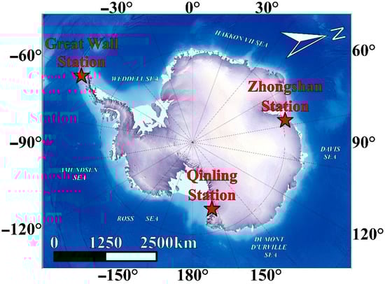
Figure 1. Spatial distribution of Great Wall Station, Qinling Station, and Zhongshan Station in Antarctica.

2.2. High-Resolution UAV Aerial Survey Data

At the local scale (1–2 km), aerodynamic roughness retrieval in this study was carried out using a Feima V100 UAV platform (Feima Robotics, Shenzhen, China) equipped with the V-CAM100 aerial survey module and the V-OP100 oblique photogrammetry module. This integrated system provides high-accuracy 3D reconstruction and multimodal remote sensing capabilities, meeting the requirements of fine-scale mapping in the complex polar environment. Prior to data acquisition, field reconnaissance, flight plan design, and control network deployment were conducted, with ground control points ensuring spatial accuracy. During the flight campaign, high-overlap imagery was collected and subsequently processed through standardized preprocessing and mosaicking to generate orthophoto Digital Orthophoto Map (DOM) and high-resolution DEM. Survey areas covered three representative sites (Great Wall Station, Zhongshan Station, and Qinling Station) with each site encompassing approximately 1.5 km × 1 km, and the data acquisition was conducted in November 2022. The UAV Aerial Survey Data is available at Zenodo [15]. Compared with satellite data, UAV-derived DEMs offer much higher resolution, capturing microtopographic variations and greatly improving the accuracy of z_0m retrieval, particularly for local-scale feature extraction and validation. However, UAV data are constrained by flight range and weather conditions, with limited coverage and higher costs of acquisition and processing. Consequently, UAV DEMs are employed in this study as high-precision benchmarks to validate satellite-derived estimates of z_0m and to assess consistency and discrepancies across different data sources.

2.3. REMA Medium-Resolution Digital Elevation Model

This study also employed the Reference Elevation Model of Antarctica (REMA), which was produced by the Polar Geospatial Center (PGC) of the United States using optical imagery at approximately 0.5 m resolution from the WorldView satellite series (WorldView-1, -2, and -3), processed through automated stereophotogrammetric algorithms. The dataset has a spatial resolution of 10 m, covers approximately 98% of the Antarctic continent, and is provided in the Antarctic Polar Stereographic projection. For z_0m retrieval at Zhongshan Station, Great Wall Station, and Qinling Station, 10 m resolution REMA tiles 36_52 and 36_53, 46_04, and 15_35 (November 2022) were selected to encompass each site and its surrounding terrain, thereby meeting the spatial requirements for regional-scale topographic characterization and z_0m estimation. REMA offers several advantages, including high resolution, broad coverage, temporal continuity, and open accessibility, making it a fundamental resource for regional-scale z_0m retrieval in polar environments. However, because it is derived from optical imagery, the dataset is susceptible to artifacts caused by cloud cover, shadows, and low solar elevation angles, which may introduce local elevation anomalies or noise. Moreover, the automated DEM generation process lacks manual refinement, leading to potential inaccuracies in fine-scale terrain details. To enhance the reliability of z_0m retrieval, REMA results in this study are compared and validated against high-resolution UAV DEM.

2.4. ICESat-2 Satellite Laser Altimetry Data

ICESat-2 was launched by NASA in September 2018 and carries the Advanced Topographic Laser Altimeter System (ATLAS). Operating in a near-polar orbit, it employs single-photon counting technology to achieve three-dimensional localization of returned photons. The raw observations have a ground footprint of about 15 m in diameter and an along-track spacing of about 0.7 m. This study uses the ATL06 elevation product, which is derived from photon data fitting and provides elevations at about 20 m spatial resolution along with slope, error estimates, and quality control information. The selected dataset spans Cycle 17 (September to December 2022), covering a complete observation cycle. For Zhongshan Station, Great Wall Station, and Qinling Station, ICESat-2 track points were extracted within about 300 × 300 km areas surrounding each site to support regional-scale z_0m retrieval. Although ATL06 has lower spatial resolution than the raw photon product (ATL03), sensitivity tests indicate that its elevation statistics are stable and representative, meeting the accuracy requirements for large-scale (Antarctic-wide) z_0m retrieval [15]. ATL06 offers broad coverage, stable accuracy, and high processing efficiency, making it well suited for regional to continental-scale topographic analysis in Antarctica. However, as an along-track laser measurement, ICESat-2 data remain spatially sparse and discontinuous, with occasional data gaps caused by cloud cover or surface reflectance conditions. Considering data quality, processing efficiency, and spatial coverage, this study adopts ATL06 as the primary ICESat-2 dataset, which is openly available from the National Snow and Ice Data Center (NSIDC, https://nsidc.org/data/ATL06, accessed on 5 June 2025).

3. Methods and Aerodynamic Roughness Retrieval Model

3.1. Raupach Drag Model Framework and Parameterization

To enable aerodynamic roughness estimation from multiple elevation datasets, this study applies the classical drag-partition model proposed by Raupach [10] as a unified retrieval framework. The model simplifies rough surfaces as arrays of obstacles and derives key aerodynamic parameters (including roughness length $z_{0\mathrm{m}}$ and displacement height $d$) from the drag imposed by these obstacles on the airflow [16].

The core idea of the model is to establish a physical relationship between wind profiles and roughness elements based on the known geometric characteristics of obstacles. In parameter extraction, the filtered elevation perturbation sequence is first analyzed, where each consecutive segment of positive values is defined as an obstacle, following the approach of Munro [9] and Andreas et al. [17]. From this, the number of obstacles within each window $f$ can be determined. The mean obstacle height H is defined as twice the standard deviation of the perturbation sequence, and the window length is denoted as $L$. The frontal area index of obstacles along the profile direction $\lambda$ is then calculated as:

$$\lambda ={\displaystyle \frac{f\cdot H}{L}}$$

(1)

Once the $\lambda$ is obtained, the displacement height $d$ can be further calculated using the following empirical formula:

$$d=H\left(1-{\displaystyle \frac{1-\mathit{exp}\left(-\sqrt{c_{d1}\lambda }\right)}{\sqrt{c_{d1}\lambda }}}\right)$$

(2)

Here, the constant $c_{d1}=7.5$, controls the functional dependence of displacement height on obstacle density, thereby representing the effective flow reference height above the roughness-element array. To further correct the logarithmic deviation of the wind profile at the obstacle top, an empirical adjustment term ${\mathit{\Psi }}_H=0.193$ is introduced.

The model partitions total drag into two components: skin friction and form drag. The skin-friction coefficient $C_s \mathrm{i}\mathrm{s} \mathrm{e}\mathrm{s}\mathrm{t}\mathrm{i}\mathrm{m}\mathrm{a}\mathrm{t}\mathrm{e}\mathrm{d} \mathrm{a}\mathrm{t} z=H$, providing a parameterization of the shear stress exerted by the wind at the obstacle top.

$$C_s(z)={\left(C_s{\left(10\right)}^{0.5}-{\displaystyle \frac{1}{k}}\left[\mathit{ln}\left({\displaystyle \frac{10-d}{H-d}}\right)-\widehat{{\mathit{\Psi }}_m\left(H\right)}\right]\right)}^{-2}$$

(3)

Here, $\kappa =0.4$ is the von Kármán constant, and $C_{s10}$ denotes the skin-friction coefficient at the reference height of 10 m, taken in this study as ${1.2071\times 10}^{-3}$. The form-drag coefficient $C_d$ is empirically parameterized as a function of obstacle height, using the piecewise fitting relationship proposed by Garbrecht et al. [18]:

$$C_d=\left\{\begin{array}{c}{\displaystyle \frac{1}{2}}\left(0.185+0.147H\right),H\le 2.5 \mathrm{m}\\ {\displaystyle \frac{1}{2}}\left(0.22\mathit{log}\left({\displaystyle \frac{H}{0.2}}\right)\right),H>2.5 \mathrm{m}\end{array}\right.$$

(4)

Once the skin-friction coefficient ($C_s)$ and form-drag coefficient $C_d$ are obtained, the dimensionless velocity ratio at the obstacle top, ${\displaystyle \frac{u\left(H\right)}{u_{\ast }}}$ can be calculated to characterize the amplification of wind speed relative to the friction velocity at the roughness-element height. This ratio is determined by iteratively solving the following implicit equation:

$$X{e}^{-x}=a$$

(5)

where $X={\displaystyle \frac{c\lambda }{2}}\cdot {\displaystyle \frac{u\left(H\right)}{u_{*}}}$, $a={\displaystyle \frac{c\lambda }{2}}{\left(C_s+\lambda C_d\right)}^{-0.5}$.

After obtaining the estimated value of ${\displaystyle \frac{u\left(H\right)}{u_{\ast }}}$, the aerodynamic roughness length $z_{0m}$ can be further inferred by inverting the logarithmic wind profile. Taking into account the displacement height $d$ and the stability correction term $\widehat{{\mathit{\Psi }}_m\left(z\right)}$, the roughness length is calculated as follows:

$$z_{0m}=\left(z-d\right)\cdot {\left[\mathit{exp}\left(\kappa \cdot {\displaystyle \frac{u\left(z\right)}{u_{\ast }}}\right)-\widehat{{\mathit{\Psi }}_m\left(z\right)}\right]}^{-1}$$

(6)

where $z$ denotes the evaluation height, taken in this study as the obstacle height $H$. Under neutral stability conditions, $\widehat{{\mathit{\Psi }}_m\left(z\right)=0}$.

The above procedure was consistently applied to perturbation profiles extracted from all three datasets used in this study (ICESat-2, REMA, and UAV), and executed independently within each sliding window. The model outputs of aerodynamic roughness length $z_{0m}$ were then mapped back to their corresponding spatial locations to generate georeferenced roughness distribution maps. This approach offers strong physical interpretability and parameter adaptability, making it suitable for roughness retrieval across different spatial scales and accuracy requirements. The specific code is available at Zenodo [19].

3.2. Aerodynamic Roughness Retrieval Method Based on UAV DEM Data

For fine-scale analysis at the local scale (1–2 km), this study employed a multirotor UAV equipped with a high-resolution imaging system to acquire DOM and DEM data with a spatial resolution finer than 0.1 m. After spatial processing and coordinate calibration, the resulting DEM products achieved high accuracy and were directly applicable for extracting microtopographic perturbations [20]. Elevation profiles were segmented into 50 m sliding windows, and perturbations were analyzed in the frequency domain. H and f were extracted from each perturbation profile and subsequently incorporated into the Raupach model to estimate aerodynamic roughness length and displacement height for each window. In addition, to verify the consistency of roughness estimates across data sources, UAV data were co-registered with ICESat-2 track elevations and REMA DEMs. Within the overlapping areas, the same model parameters were applied for comparative analysis, enabling quantification of retrieval accuracy and applicable scales for each dataset.

3.3. Aerodynamic Roughness Retrieval Method Based on REMA Data

To characterize aerodynamic roughness at the regional scale, this study used 10 m resolution DEMs from REMA in combination with the Raupach drag-partition model. Unlike the along-track elevation profiling approach applied to ICESat-2, this method generates one-dimensional profiles directly from the two-dimensional elevation grid, eliminating the need for photon denoising and track fitting, and thus providing a more streamlined and efficient workflow.

In practice, elevation profiles were extracted in both the transverse and longitudinal directions of the study area, and each profile was detrended and smoothed. A high-pass filter was then applied to selectively enhance short-wavelength (<35 m) topographic signals while attenuating long-wavelength (>35 m) background components. The filtered perturbation profiles were divided into 50 m sliding windows, from which H was extracted and f was calculated. Finally, aerodynamic roughness length was estimated using the Raupach model, and results from all profiles were combined to generate regional-scale roughness distribution maps.

3.4. Aerodynamic Roughness Retrieval Method Based on ICESat-2 Data

This study builds on a previously proposed track-processing framework, with several improvements introduced to enhance data quality and processing stability [5]. In the preprocessing stage, high-quality elevation data were first extracted from the strong-beam tracks within the geographic extent of the study area. To eliminate outliers, median absolute deviation (MAD) filtering was applied to the elevation profiles using a 50 m sliding window. Local medians and deviation thresholds were computed, and asymmetric upper and lower limits were applied to remove points with large deviations from the median, thereby ensuring the continuity of the track profiles.

The processed track data were segmented using 2 km sliding windows. Within each segment, cumulative distances were calculated from the latitude and longitude of track points to construct along-track elevation profiles. The discrete track points were then interpolated onto a uniform 1 m grid using one-dimensional ordinary kriging. A Gaussian covariance model with a 30 m range was applied, and only the nearest track points around each interpolation location were used to improve estimation accuracy.

High-pass filtering was applied to the interpolated profiles to remove long-wavelength topographic trends (>35 m). This scale separation was performed in the frequency domain using a Fourier transform. The transform decomposes the one-dimensional elevation profile into its constituent sinusoidal waves of different wavelengths, enabling us to apply a sharp cut-off filter that attenuates all spectral components with wavelengths longer than 35 m. Before performing the Fourier transform, the track profiles were mirrored to generate periodic sequences, thereby effectively suppressing spectral leakage in the extraction of high-frequency perturbations. The resulting high-pass filtered residual profiles were then used to identify microtopographic obstacle structures and to extract perturbation parameters, which served as inputs for roughness retrieval.

Obstacle height (H) was defined as twice the standard deviation of the high-pass residual sequence, with consecutive positive perturbations treated as individual obstacle elements. The number of obstacles was obtained by direct counting. Based on obstacle height and number, λ per unit track length was calculated and incorporated into the Raupach model [10] to estimate aerodynamic roughness length (z_0m), displacement height (d), and drag ratios. These results were then mapped to produce the spatial distribution of roughness around each station.

The three types of data used in this study possess distinct temporal characteristics and update frequencies. UAV data are obtained through field campaigns, and their acquisition times depend on specific experimental schedules. The REMA DEM is a static elevation model representing the averaged topographic state of a specific historical period. The ICESat-2 satellite laser altimetry mission operates on a 91-day full repeat cycle, providing sustained observations globally. The overall workflow for aerodynamic roughness retrieval, incorporating the parallel processing of UAV, REMA DEM, and ICESat-2 data, is summarized in Figure 2.

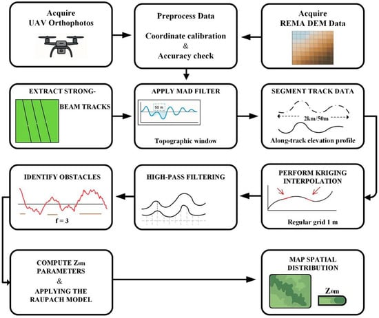
Figure 2. Flowchart of the Aerodynamic Roughness Retrieval Model.

4. Results

4.1. Aerodynamic Roughness Retrieval Results Based on UAV Data

z_0m in the Great Wall Station region varies systematically with surface types, being lowest over water and highest over coastal bedrock. The area is characterized by extensive bare soil, together with exposed bedrock, patches of snow, small water bodies, and sparse vegetation in the gentler inland zones. In Figure 3a, coastal water appears as a dark-toned feature with sharp boundaries. The shoreline consists mainly of bedrock, while the inland surface is dominated by bare soil interspersed with snow and occasional vegetation. In Figure 3d, water surfaces correspond to extremely low z_0m values (<0.0001 m). Snow-covered areas show z_0m values between 0.001 and 0.01 m. Bare soil and vegetated zones, which occupy the largest and relatively gentle portions of the terrain, exhibit lower values ranging from about 0.0002 to 0.5 m. In contrast, coastal bedrock displays the highest z_0m values (0.001–1 m), reflecting the influence of surface roughness elements and topographic relief on near-surface airflow. Overall, z_0m in the Great Wall Station region shows a clear spatial correspondence with surface types, with water being the lowest, snow and bare soil relatively low, and bedrock the highest. This distribution agrees well with UAV results, demonstrating the ability of our method to resolve microtopographic effects: it can both distinguish the levels of z_0m across different surface types and capture boundary transitions consistent with imagery [11]. The agreement in heterogeneous terrains further supports the reliability of this approach under complex surface conditions [11].

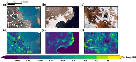
Figure 3. Site-scale surface imagery and aerodynamic roughness length (z_0m) maps derived from high-resolution UAV imagery. Panels (a–c) show the orthophotos of Great Wall Station, Qinling Station, and Zhongshan Station, respectively; panels (d–f) present the corresponding spatial distributions of aerodynamic roughness length (z_0m), with color gradients from purple (low) to yellow (high) indicating variations in roughness magnitude.

z_0m shows a strong dependence on terrain relief, with elevated values over coastal bedrock and generally lower values across inland surfaces at Qinling Station. The surface at Qinling Station consists of a mixture of bedrock, snow, and bare soil. As shown in Figure 3e, z_0m exceeds 0.1 m over coastal bedrock, whereas inland gravel and snow surfaces display smaller differences, with values generally ranging from 0.0002 to 0.1 m. This pattern reflects the influence of protruding terrain on near-surface airflow, consistent with the finding that roughness increases exponentially with obstacle height and density [19]. It also illustrates the capacity of the Raupach model to capture the impact of form drag under rugged conditions [5]. In contrast, gently sloping bare soil surfaces show z_0m values of about 0.0002–0.005 m, while snow-covered areas remain below 0.1 m. Overall, Qinling Station is the site where z_0m shows the closest correspondence with terrain relief among the three Antarctic stations.

z_0m ranges from 10⁻⁴ to over 0.5 m, with the highest values on rugged bedrock terrain and a clear correspondence to topographic relief at Zhongshan Station. The region in and around Zhongshan Station features diverse surface types and complex topography, including coastal ice, exposed bedrock, and residual snow cover. Figure 3c clearly illustrates their spatial distribution, where coastal ice forms a sharp boundary with adjacent snow patches and surrounding rock outcrops. In Figure 3f, water surfaces appear in purple with extremely low z_0m values (<0.0001 m), consistent with their smooth and flat characteristics. Bedrock is predominantly shown in green to yellow, corresponding to z_0m values of about 0.001–0.5 m, reflecting the strong influence of rugged terrain on near-surface airflow. Marked distinctions in z_0m among surface types are consistent with observations from other Antarctic regions, where snow-covered areas typically exhibit z_0m < 0.01 m and appear bluish purple [21,22]. Overall, z_0m at Zhongshan Station spans a broad range, from 10⁻⁴ m to beyond 0.5 m. Higher values are generally associated with areas of pronounced terrain variability, where local z_0m can approach 1 m, underscoring the pronounced effect of terrain-induced roughness.

In summary, the three stations show that z_0m distribution corresponds closely to surface type and topographic variability: the lowest values occur over water (<0.0001 m), relatively low values over snow (0.0002–0.01 m), and higher values over bedrock or gravel surfaces (0.001–1 m, locally exceeding 1 m). At Great Wall Station, snow dominates, resulting in generally low and relatively uniform values. At the Qinling Station, rugged terrain and extensive bedrock exposures produce numerous high-value patches, particularly along ridges, steep slopes, and snow–rock boundaries where sharp z_0m transitions appear. At Zhongshan Station, the wide range of surface types leads to a broader spread of values. These differences reflect the drag imposed by terrain roughness and obstacles such as bedrock, snow surfaces, and bare soil: taller and denser roughness elements yield higher z_0m, while smoother surfaces yield lower values. This spatial pattern has been confirmed by both remote sensing and in situ observations in Greenland and at multiple Antarctic sites [11,21], underscoring the important role of geomorphology and topography in shaping z_0m [19].

In addition, this study analyzes the relationship between z_0m, elevation, and slope. At Great Wall Station, z_0m shows considerable spatial variability and corresponds closely to terrain variation. The elevation map (Figure 4a) indicates higher terrain in the south (locally reaching 143 m) and lower, relatively flat coastal areas in the north. Accordingly, high z_0m values are mostly concentrated in the southern zones of steep bedrock and gravel, while low values dominate in the northern coastal belt and flatter snow-covered areas, as depicted in Figure 3d. Overall, according to the slope map in Figure 4d, steeper slopes and more rugged surfaces are more likely to exhibit higher z_0m, whereas regions with gentle slopes and smoother surfaces generally show lower values, consistent with the spatial pattern observed in Figure 3d. UAV-based studies further demonstrate that z_0m retrievals are more robust in steep-slope areas and less sensitive to parameter settings or sampling strategies [11]. These findings suggest that slope and terrain variability increase the height and density of roughness elements, enhancing form drag and turbulence, thereby raising z_0m and amplifying its spatial heterogeneity. This makes topographic slope an important factor controlling z_0m distribution.

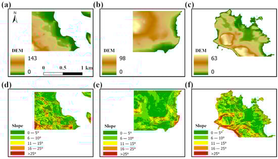
Figure 4. Topographic characteristics of Great Wall Station, Qinling Station, and Zhongshan Station, showing the spatial distribution of elevation and slope across the three study areas located along the Antarctic coastal region. In the elevation maps, brown indicates higher terrain and green indicates lower terrain; in the slope maps, green represents gentle slopes (0–5°), while red represents steep slopes (>25°). Specifically, panels (a,d) show the elevation and slope maps for Great Wall Station, (b,e) for Qinling Station, and (c,f) for Zhongshan Station.

z_0m is mostly low and quite even, consistent with the low elevation, mild slopes, and wide snow cover near Qinling Station. Figure 4b shows that elevation ranges from 0 to 98 m, with overall flat terrain and minimal variability. Figure 4e indicates that Most slopes are gentle (0–10°), with only a few steeper sections (>25°). In these steeper areas, z_0m rises to about 0.1–1 m. Overall, the predominance of gentle slopes accounts for the uniformly low z_0m, while localized slope breaks produce slightly higher values (Figure 3e). Similarly, Alekseychik et al. (2017) [23] reported in Arctic wetlands that even small surface undulations (<0.5 m) can significantly affect z_0m, particularly when wind direction aligns with slope orientation.

z_0m displays high values with wide variability at Zhongshan Station. The elevation map in Figure 4c reveals pronounced topographic variation, with altitudes ranging from 0 to 63 m and clear surface undulations. Rugged terrain is characterized by large z_0m values, whereas flatter areas correspond to smaller values (Figure 3f). The slope map in Figure 4f further highlights widespread steep slopes (>25°), particularly along bedrock margins and distinct sea-ice boundaries, where z_0m approaches 0.1 m. Such slopes strongly disturb near-surface airflow, directly contributing to substantial z_0m. Previous studies have shown that on ice or bedrock with pronounced slope variations, local z_0m values can differ by a factor of two to three [22,24].

Overall, the three stations indicate that spatial differences in elevation and slope directly shape the distribution of z_0m. Areas with steep slopes and pronounced terrain relief, such as Great Wall Station and Zhongshan Station, are characterized by larger z_0m values, whereas the gentler terrain at Qinling Station corresponds to lower values (elevation and slope information from Figure 4, z_0m distribution from Figure 3d–f). This highlights slope and surface obstacles as key factors influencing z_0m with more complex microtopography exerting a stronger impact on energy exchange and airflow.

4.2. Aerodynamic Roughness Inversion Based on REMA Data

This section analyzes z_0m across three Antarctic stations using REMA data, examining its relationship with overall topography and glacier dynamics. z_0m is generally low but increases at island margins and exposed rock surfaces in the Great Wall Station area (Figure 5b). Snow and ice cover most of the islands, leaving only small areas of exposed rock (Figure 5a). Overall, z_0m remains within 10⁻⁴–10⁻³ m (Figure 5b), consistent with estimates from three-dimensional point cloud data over Arctic ice, which showed that smooth snow and ice surfaces typically exhibit values below 10⁻³ m [17]. In contrast, values increase to the order of 10⁻² m along island edges and rock outcrops (Figure 5b). This pattern reflects the enhanced aerodynamic resistance generated by terrain protrusions and exposed rock. Similar patterns were reported from field measurements over Alpine glaciers, where ice–rock mixed zones and debris-covered areas produced higher z_0m values (10⁻³–10⁻² m) compared to snow-covered surfaces [25].

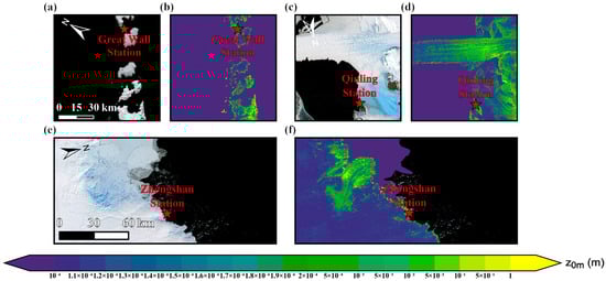
Figure 5. Landsat Image Mosaic of Antarctica (LIMA) satellite imagery and aerodynamic roughness length (z_0m) maps derived from REMA data. Panels (a,c,e) show the orthorectified satellite images of Great Wall Station, Qinling Station, and Zhongshan Station, respectively; panels (b,d,f) present the corresponding spatial distribution of aerodynamic roughness length (z_0m), with color gradients from purple (low values) to yellow (high values) indicating variations in surface roughness.

In the Qinling Station region, z_0m is characterized by high values and pronounced spatial variability. According to Figure 5d, z_0m often exceeds 0.05 m occur along bare-rock ridges and steep slopes, while lower values below 0.01 m dominate snow-covered or gentle-slope areas, giving an overall range of 10⁻⁴ to 0.1 m. Glacier activity is frequent in this region, and z_0m is typically high (>0.05 m) along glacier surfaces and ice–rock boundaries. This is because glacier flow and deformation create ridges, crevasses, and fractures that increase surface irregularity and thereby enhance form drag. Such structural disturbances have also been well documented in studies on roughness variability under glacier dynamics [23,26]. In contrast, sea-ice areas are characterized by low z_0m, as their smooth, nearly level surfaces contain few obstacles and exert little resistance on airflow.

z_0m shows a clear decline from the coast toward the interior (Figure 5f). As shown in Figure 5f, coastal waters and flat snow-covered surfaces have low values (0.0001–0.0002 m), while bedrock and gravel show much higher values (0.01–0.5 m) in the Zhongshan Station region. In coastal zones with exposed rock and gravel beaches, z_0m exceeds 10⁻² m, reflecting the stronger aerodynamic drag imposed by surface irregularities and rock distributions. Further inland, z_0m rapidly decreases to 10⁻⁴–10⁻³ m (Figure 5f), consistent with the smoother surface of the ice sheet and its weaker resistance to airflow. A similar spatial pattern has been reported for glacier surfaces on the Tibetan Plateau [27]. Distinct geomorphic boundaries, such as ice margins and ice–plain transitions, were associated with abrupt shifts in roughness, illustrating a typical topographic control mechanism.

Overall, the REMA-based analysis shows that the spatial distribution of z_0m at the three stations is strongly influenced by geomorphology and glacier dynamics. As shown in Figure 5b, at Great Wall Station, z_0m is the lowest, reflecting the weak aerodynamic disturbance of island terrain and smooth snow- and ice-covered surfaces [17,28]. At Qinling Station, z_0m is the highest and most variable (Figure 5d), underscoring the strong impact of glacier dynamics on surface roughness [23,26]. At Zhongshan Station, z_0m is higher along the coast and decreases inland (Figure 5f), forming a transitional pattern that demonstrates the influence of geomorphic and topographic complexity on roughness distribution [25,27]. These findings emphasize the key role of topography and glacier dynamics in shaping the spatial variability of z_0m and provide important insights into Antarctic wind structures and surface energy exchange [29].

4.3. Aerodynamic Roughness Inversion Results Based on ICESat-2 Data

ATL03 data provide a high resolution of about 1 m, but processing the full Antarctic dataset involves prohibitive computational costs. To improve efficiency, we incorporated the ATL06 product, with a coarser resolution of about 20 m, for z_0m retrieval. Since different datasets may result in discrepancies, we conducted a sensitivity experiment along a representative track, comparing ATL06 and ATL03 results across five window lengths (200 m, 1 km, 2 km, 4 km, and 8 km). The results show that the error decreases and then increases with window size, reaching a minimum at 2 km, where the root mean square error (RMSE) between ATL06 and ATL03 is only 7.45 × 10⁻⁶ m (Table 1). The findings in Table 1 indicate that the 2000 m window is a justified choice (Table 1).

Table 1. Root mean square error (RMSE) between ATL06 and ATL03 at different window lengths.

Window Length (m)	200	1000	2000	4000	8000
RMSE (m)	9.83 × 10−6	7.86 × 10−6	7.45 × 10−6	15.8 × 10−6	54.0 × 10−6

Figure 6 presents the preliminary spatial distribution of z_0m retrieved from ICESat-2 data, shown as discrete points over the Great Wall Station, the Qinling Station, and the Zhongshan Station, with color indicating z_0m magnitude. While ICESat-2 provides high precision, its sparse coverage captures only discrete z_0m features along the satellite tracks [30]. In the Qinling Station area, where tracks are denser, z_0m spans a broad range of values, revealing the effects of microtopographic variability on surface roughness [31]. To improve spatial continuity and generate a spatially complete map, a continuous z_0m field was produced by applying inverse distance weighting (IDW) interpolation to the discrete ICESat-2 point measurements. This deterministic method assigns weights to neighboring points inversely proportional to their distance (typically to the power of p = 2), ensuring that closer points exert greater influence on the estimated value. The resulting interpolated map is presented in Figure 7. Figure 7a–c displays satellite imagery for each region, and Figure 7d–f the corresponding z_0m distribution. Colors transition from purple (low) to yellow (high), reflecting a wide range of values and marked local transitions: high values occur primarily over bedrock and steep slopes, while low values are concentrated over water and flat snow surfaces. At snow–rock boundaries, z_0m increases gradually from low to high [32]. In the Great Wall Station region, most z_0m values range between 10⁻³ and 10⁻² m and appear in strip or patch patterns. Higher values occur near coasts and topographic protrusions, locally reaching 0.05 m. The Qinling Station region shows the greatest spatial variability, with values extending from below 10⁻³ m to above 0.05 m. Elevated values are concentrated along glaciers, ridges, and exposed rock, forming distinct bands. At Zhongshan Station, z_0m generally lies between the other two regions, typically 10⁻³–10⁻² m, higher near the coast and lower inland. Figure 7 illustrates this coastal-to-interior transition toward smoother ice surfaces [33]. Interpolation not only fills observational gaps but also provides a more intuitive representation of aerodynamic roughness distribution. These patterns closely match those inferred from REMA data, confirming that geomorphology, terrain relief, and glacier activity are the dominant controls on z_0m across different Antarctic environments [34] (Geng et al., 2021).

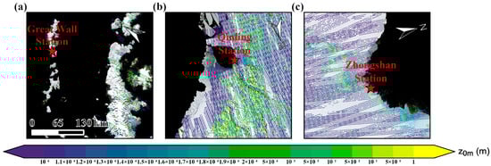
Figure 6. z_0m derived from ICESat-2 trajectories. Panels (a–c) correspond to the regions around Great Wall Station, Qinling Station, and Zhongshan Station, respectively. The color gradient from purple (low) to yellow (high) indicates variations in roughness magnitude.

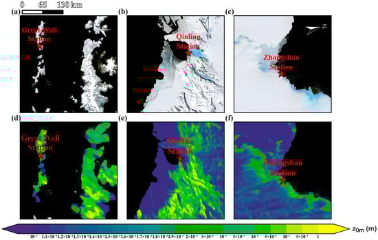
Figure 7. Spatial distribution of aerodynamic roughness length (z_0m) based on ICESat-2 data. Panels (a–c) show satellite imagery of the corresponding regions, while panels (d–f) display the associated aerodynamic roughness length maps. The color gradient from purple (low) to yellow (high) indicates variations in roughness magnitude.

4.4. Comparison and Validation of Inversion Accuracy

This study compares and validates aerodynamic roughness length (z_0m) retrievals from different datasets (UAV, REMA, and ICESat-2). Using UAV data as the reference, the z_0m values at Zhongshan Station, Great Wall Station, and Qinling Station are 6.0 × 10⁻⁴ m, 7.1 × 10⁻⁴ m, and 3.4 × 10⁻⁴ m, respectively. The REMA-derived results are generally consistent with the UAV measurements: slightly underestimated at Zhongshan Station (5.3 × 10⁻⁴ m) and Great Wall Station (5.4 × 10⁻⁴ m), and slightly overestimated at Qinling Station (4.5 × 10⁻⁴ m). ICESat-2 data perform well at Great Wall Station (9.0 × 10⁻⁴ m), show a slight overestimation at Qinling Station (7.4 × 10⁻⁴ m), and a slight underestimation at Zhongshan Station (2.1 × 10⁻⁴ m). The comparative summary of the z_0m values across all stations is presented in Table 2. Overall, the aerodynamic roughness lengths obtained from the three datasets are consistent in order of magnitude, indicating good agreement.

Table 2. z_0m (m) from UAV, REMA, and ICESat-2 at three Antarctic stations.

Over Bare	UAV	REMA	ICESat-2
Great Wall Station	7.1 × 10−4	5.4 × 10−4	9.0 × 10−4
Qinling Station	3.4 × 10−4	4.5 × 10−4	7.4 × 10−4
Zhongshan Station	6.0 × 10−4	5.3 × 10−4	2.1 × 10−4

Thanks to their high spatial resolution and accuracy, UAV data are best suited for fine-scale characterization of z_0m. REMA data provide reliable estimates on the scale of hundreds of kilometers, while ICESat-2 data are more appropriate for continental-scale analysis. Integrating the three datasets enhances the robustness of z_0m estimation and enables accurate assessment across multiple spatial scales.

5. Discussion

To ensure the comparability of z_0m estimates derived from UAV, ATL06, and REMA datasets, the two-dimensional UAV DEM was converted into 200 m × 15 m linear profiles. This process standardizes the data dimensionality and morphological representation across the different sources. The profiles were then processed using identical high-pass filtering and parameter extraction procedures. This methodological alignment guarantees that the ensuing estimation and comparison are based on consistent characterization of surface obstacles, thereby minimizing biases introduced by data resolution and processing techniques. In validating the results, UAV-derived estimates, owing to their superior spatial resolution, serve as a high-accuracy reference for error evaluation and accuracy comparison against ATL06 and REMA retrievals, thereby enhancing the reliability of z_0m estimates. Therefore, the UAV approach not only resolves the difficulties of inconsistent parameters and scale conversion in traditional Structure-from-Motion methods, but also broadens its application to Antarctic surface studies and multi-dataset comparisons.

Despite its high accuracy and wide availability, the Reference Elevation Model of Antarctica (REMA) has not been systematically employed for physically based retrieval of z_0m. Previous applications have been limited to approximating roughness via simple terrain metrics, leaving its potential for deriving this key aerodynamic parameter unexplored. A common reliance on empirical scale indices has resulted in a lack of model-driven roughness definition and estimation, alongside significant inconsistencies in parameter choices and scale partitioning that prevent consistent cross-data analysis. In this study, REMA is, for the first time, incorporated into a Raupach-model-based framework for systematic extraction and estimation of z_0m structural parameters, using a workflow kept fully consistent with ICESat-2 processing. High-pass filtering is applied to isolate surface perturbations, obstacle height is uniformly defined as 2σ_z, and obstacle number is derived from the statistics of continuous positive-perturbation segments. This workflow ensures that REMA and ATL06 share identical model structures and parameter definitions in z_0m estimation, thereby enabling direct comparison between the two datasets.

The drag-partition model of Raupach [10] was first combined with ICESat-2 ATL03 photon cloud data to estimate z_0m over ice sheets [5]. However, their approach relies on track-by-track interpolation of dense photon points, which is computationally intensive and susceptible to errors when data quality is degraded. In response, this study leverages the ATL06 elevation product as the primary dataset. With its 20 m resolution, consistent accuracy, and computational efficiency, ATL06 is well-suited for this application within an unchanged model framework. These attributes collectively enable an accurate retrieval of z_0m from ICESat-2 data at a regional scale. The ATL06 product provides pre-processed, fitted, and continuous elevation profiles. This ready-to-use format permits the direct construction of 2 km analysis windows for profile extraction, streamlining the entire workflow. In processing, we detrend linearly and apply a 35 m high-pass filter to remove background topography and isolate small-scale surface perturbations. Obstacle height (H) is defined as twice the standard deviation, while obstacle number is determined from continuous segments of positive elevation perturbations to calculate λ. To further improve model adaptability to real ice-surface conditions, we adopt the Cd(H) parameterization scheme, which adjusts drag intensity according to obstacle geometry [18]. The method presented here moves beyond earlier approaches, which were often limited by empirical constants or fixed structural assumptions. It successfully preserves physical realism while simultaneously achieving substantial gains in processing efficiency and applicability. This advancement enables ICESat-2 to support large-scale z_0m estimation and spatial distribution analysis across extensive tracks and regions.

The temporal coverage frequency of different data sources directly influences their ability to characterize the dynamic changes in z_0m. Although drone surveys can obtain high spatial resolution observational data, their updates typically rely on irregular fieldwork, which limits their temporal continuity and coverage. REMA are similarly constrained by station distribution and maintenance cycles, making it challenging to achieve large-scale, standardized, and continuous monitoring. In contrast, the ICESat-2 satellite achieves high-precision sampling of the global surface through its along-track laser footprints, with a regular and predictable 91-day revisit cycle. This unique spatiotemporal sampling capability enables ICESat-2 to provide large-scale, standardized, and temporally consistent observational data, thereby supporting the dynamic monitoring of aerodynamic roughness from seasonal to interannual scales. Therefore, in constructing long-term, dynamically updated surface roughness datasets, ICESat-2 offers irreplaceable advantages in terms of data update frequency, coverage, and consistency, providing critical support for transforming surface roughness from a static parameter into a dynamic scientific variable that reflects surface processes and changes.

6. Conclusions and Prospects

Based on the drag-partition model of Raupach [10], this study introduces a multi-source remote sensing framework for z_0m and applies it to three Antarctic sites: Zhongshan Station, Great Wall Station, and Qinling Station. The results show clear differences in both the magnitude and spatial structure of z_0m among the stations. Across increasing spatial scales, the UAV, REMA, and ICESat-2 datasets offer complementary strengths: high-precision benchmarking (UAV), regional stability (REMA), and continental-scale z_0m estimation (ICESat-2). By combining these datasets, the framework achieves a balance between accuracy, spatial resolution, and coverage, offering a robust solution for z_0m estimation across scales in Antarctica. This approach provides essential support for polar boundary-layer modeling and surface energy balance studies.

While the study provides important insights, several aspects still warrant further improvement. The current analysis relies on static elevation data and does not account for the seasonal dynamics of ice surfaces. Earlier studies have shown that coastal regions exhibit pronounced seasonal contrasts in snow cover and bare-ice exposure, which may cause temporal variability in z_0m. Seasonal- and interannual-scale time-series remote sensing data provide new opportunities to advance dynamic modeling of z_0m. In addition, this work focuses on three representative sites, and its spatial representativeness remains limited. Future efforts should extend validation to other Antarctic coastal zones and characteristic landforms, and include uncertainty assessments, to further enhance the generalizability and practical value of the framework.

References

- Golledge, N.R.; Keller, E.D.; Gomez, N.; Naughten, K.A.; Bernales, J.; Trusel, L.D.; Edwards, T.L. Global Environmental Consequences of Twenty-First-Century Ice-Sheet Melt. Nature 2019, 566, 65–72. [Google Scholar] [CrossRef]
- Otosaka, I.N.; Shepherd, A.; Ivins, E.R.; Schlegel, N.-J.; Amory, C.; van den Broeke, M.R.; Horwath, M.; Joughin, I.; King, M.D.; Krinner, G.; et al. Mass Balance of the Greenland and Antarctic Ice Sheets from 1992 to 2020. Earth Syst. Sci. Data 2023, 15, 1597–1616. [Google Scholar] [CrossRef]
- Hock, R. Glacier Melt: A Review of Processes and Their Modelling. Prog. Phys. Geogr. 2005, 29, 362–391. [Google Scholar] [CrossRef]
- Munro, D.S. Surface Roughness and Bulk Heat Transfer on a Glacier: Comparison with Eddy Correlation. J. Glaciol. 1989, 35, 343–348. [Google Scholar] [CrossRef]
- Quincey, D.; Smith, M.; Rounce, D.; Ross, A.; King, O.; Watson, C. Evaluating Morphological Estimates of the Aerodynamic Roughness of Debris Covered Glacier Ice. Earth Surf. Process. Landf. 2017, 42, 2541–2553. [Google Scholar] [CrossRef]
- van Tiggelen, M.; Smeets, P.C.J.P.; Reijmer, C.H.; Wouters, B.; Steiner, J.F.; Nieuwstraten, E.J.; Immerzeel, W.W.; van den Broeke, M.R. Mapping the Aerodynamic Roughness of the Greenland Ice Sheet Surface Using ICESat-2: Evaluation over the K-Transect. Cryosphere 2021, 15, 2601–2621. [Google Scholar] [CrossRef]
- Cheng, F.; Yang, Q.; Liu, C.; Han, B.; Peng, S.; Hao, G. Evaluating Parameterizations for Turbulent Fluxes over the Landfast Sea-Ice Surface in Prydz Bay, Antarctica. Adv. Atmos. Sci. 2023, 40, 1816–1832. [Google Scholar] [CrossRef]
- Smeets, C.J.P.P.; van den Broeke, M.R. Temporal and Spatial Variations of the Aerodynamic Roughness Length in the Ablation Zone of the Greenland Ice Sheet. Bound.-Layer Meteorol. 2008, 128, 315–338. [Google Scholar] [CrossRef]
- Lettau, B. The Transport of Moisture into the Antarctic Interior. Tellus 1969, 21, 331–340. [Google Scholar] [CrossRef]
- Raupach, M.R. Drag and Drag Partition on Rough Surfaces. Bound.-Layer Meteorol. 1992, 60, 375–395. [Google Scholar] [CrossRef]
- Dachauer, A.; Hann, R.; Hodson, A.J. Aerodynamic Roughness Length of Crevassed Tidewater Glaciers from UAV Mapping. Cryosphere 2021, 15, 5513–5528. [Google Scholar] [CrossRef]
- van Tiggelen, M.; Smeets, P.C.J.P.; Reijmer, C.H.; van den Broeke, M.R.; van As, D.; Box, J.E.; Fausto, R.S. Observed and Parameterized Roughness Lengths for Momentum and Heat Over Rough Ice Surfaces. J. Geophys. Res. Atmos. 2023, 128, e2022JD036970. [Google Scholar] [CrossRef]
- Mosadegh, E.; Nolin, A.W. A New Data Processing System for Generating Sea Ice Surface Roughness Products from the Multi-Angle Imaging SpectroRadiometer (MISR) Imagery. Remote Sens. 2022, 14, 4979. [Google Scholar] [CrossRef]
- Scanlan, K.M.; Rutishauser, A.; Simonsen, S.B. Greenland Ice Sheet Surface Roughness from Ku- and Ka-Band Radar Altimetry Surface Echo Strengths. Cryosphere 2025, 19, 1221–1239. [Google Scholar] [CrossRef]
- Sun, Y. UAV DEM Data from Zhongshan, Great Wall, and Qinling Stations in Antarctica [Data Set]. Zenodo 2025a. Available online: https://zenodo.org/records/17093633 (accessed on 5 June 2025).
- Brunt, K.M.; Neumann, T.A.; Smith, B.E. Assessment of ICESat-2 Ice Sheet Surface Heights, Based on Comparisons Over the Interior of the Antarctic Ice Sheet. Geophys. Res. Lett. 2019, 46, 13072–13078. [Google Scholar] [CrossRef]
- Andreas, E.L. Air-ice Drag Coefficients in the Western Weddell Sea: 2. A Model Based on Form Drag and Drifting Snow. J. Geophys. Res. Ocean. 1995, 100, 4833–4843. [Google Scholar] [CrossRef]
- Smith, M.W.; Quincey, D.J.; Dixon, T.; Bingham, R.G.; Carrivick, J.L.; Irvine-Fynn, T.D.L.; Rippin, D.M. Aerodynamic Roughness of Glacial Ice Surfaces Derived from High-resolution Topographic Data. J. Geophys. Res. Earth Surf. 2016, 121, 748–766. [Google Scholar] [CrossRef]
- Garbrecht, T.; Lüpkes, C.; Hartmann, J.; Wolff, M. Atmospheric Drag Coefficients over Sea Ice—Validation of a Parameterisation Concept. Tellus A Dyn. Meteorol. Oceanogr. 2002, 54, 205–219. [Google Scholar] [CrossRef]
- Sun, Y. Aerodynamic Roughness Retrieval Model at Typical Antarctic Stations Based on Multi-Source Remote Sensing. [Code]. Zenodo 2025b. Available online: https://zenodo.org/records/17181747 (accessed on 5 June 2025).
- James, M.R.; Robson, S. Mitigating Systematic Error in Topographic Models Derived from UAV and Ground-based Image Networks. Earth Surf. Process. Landf. 2014, 39, 1413–1420. [Google Scholar] [CrossRef]
- Guo, S.; Chen, R.; Liu, G.; Han, C.; Song, Y.; Liu, J.; Yang, Y.; Liu, Z.; Wang, X.; Liu, X.; et al. Simple Parameterization of Aerodynamic Roughness Lengths and the Turbulent Heat Fluxes at the Top of Midlatitude August-One Glacier, Qilian Mountains, China. J. Geophys. Res. Atmos. 2018, 123, 12066–12080. [Google Scholar] [CrossRef]
- Reijmer, C.H.; Van Meijgaard, E.; Van Den Broeke, M.R. Numerical Studies with a Regional Atmospheric Climate Model Based on Changes in the Roughness Length for Momentum and Heat over Antarctica. Bound.-Layer Meteorol. 2004, 111, 313–337. [Google Scholar] [CrossRef]
- Weiss, A.I.; King, J.; Lachlan-Cope, T.; Ladkin, R. On the Effective Aerodynamic and Scalar Roughness Length of Weddell Sea Ice. J. Geophys. Res. 2011, 116, D19119. [Google Scholar] [CrossRef]
- Alekseychik, P.K.; Korrensalo, A.; Mammarella, I.; Vesala, T.; Tuittila, E.S. Relationship between aerodynamic roughness length and bulk sedge leaf area index in a mixed-species boreal mire complex. Geophys. Res. Lett. 2017, 16, 5836–5843. [Google Scholar] [CrossRef]
- Fassnacht, S.R.; Suzuki, K.; Nemoto, M.; Sanow, J.E.; Kosugi, K.; Tedesche, M.E.; Frey, M.M. Location Dictates Snow Aerodynamic Roughness. Glacies 2024, 1, 1–16. [Google Scholar] [CrossRef]
- Brock, B.W.; Willis, I.C.; Sharp, M.J. Measurement and Parameterization of Aerodynamic Roughness Length Variations at Haut Glacier d’Arolla, Switzerland. J. Glaciol. 2006, 52, 281–297. [Google Scholar] [CrossRef]
- Chambers, J.R.; Smith, M.W.; Quincey, D.J.; Carrivick, J.L.; Ross, A.N.; James, M.R. Glacial Aerodynamic Roughness Estimates: Uncertainty, Sensitivity, and Precision in Field Measurements. J. Geophys. Res. Earth Surf. 2020, 125, e2019JF005167. [Google Scholar] [CrossRef]
- Munevar Garcia, S.; Miller, L.E.; Falcini, F.A.M.; Stearns, L.A. Characterizing Bed Roughness on the Antarctic Continental Margin. J. Glaciol. 2023, 69, 2114–2125. [Google Scholar] [CrossRef]
- Liu, J.; Chen, R.; Han, C. Spatial and Temporal Variations in Glacier Aerodynamic Surface Roughness during the Melting Season, as Estimated at the August-One Ice Cap, Qilian Mountains, China. Cryosphere 2020, 14, 967–984. [Google Scholar] [CrossRef]
- Andreas, E.L. A Relationship between the Aerodynamic and Physical Roughness of Winter Sea Ice. Q. J. R. Meteorol. Soc. 2011, 137, 1581–1588. [Google Scholar] [CrossRef]
- Howat, I.M.; Porter, C.; Smith, B.E.; Noh, M.-J.; Morin, P. The Reference Elevation Model of Antarctica. Cryosphere 2019, 13, 665–674. [Google Scholar] [CrossRef]
- Herzfeld, U.C.; Trantow, T.; Lawson, M.; Hans, J.; Medley, G. Surface Heights and Crevasse Morphologies of Surging and Fast-Moving Glaciers from ICESat-2 Laser Altimeter Data—Application of the Density-Dimension Algorithm (DDA-Ice) and Evaluation Using Airborne Altimeter and Planet SkySat Data. Sci. Remote Sens. 2021, 3, 100013. [Google Scholar] [CrossRef]
- Enderlin, E.M.; Elkin, C.M.; Gendreau, M.; Marshall, H.P.; O’Neel, S.; McNeil, C.; Florentine, C.; Sass, L. Uncertainty of ICESat-2 ATL06- and ATL08-Derived Snow Depths for Glacierized and Vegetated Mountain Regions. Remote Sens. Environ. 2022, 283, 113307. [Google Scholar] [CrossRef]
- Geng, T.; Zhang, S.; Xiao, F.; Li, J.; Xuan, Y.; Li, X.; Li, F. DEM Generation with ICESat-2 Altimetry Data for the Three Antarctic Ice Shelves: Ross, Filchner–Ronne and Amery. Remote Sens. 2021, 13, 5137. [Google Scholar] [CrossRef]
- Li, T.; Dawson, G.J.; Chuter, S.J.; Bamber, J.L. A High-Resolution Antarctic Grounding Zone Product from ICESat-2 Laser Altimetry. Earth Syst. Sci. Data 2022, 14, 535–557. [Google Scholar] [CrossRef]
- Markus, T.; Neumann, T.; Martino, A.; Abdalati, W.; Brunt, K.; Csatho, B.; Farrell, S.; Fricker, H.; Gardner, A.; Harding, D.; et al. The Ice, Cloud, and Land Elevation Satellite-2 (ICESat-2): Science Requirements, Concept, and Implementation. Remote Sens. Environ. 2017, 190, 260–273. [Google Scholar] [CrossRef]
Disclaimer/Publisher’s Note: The statements, opinions and data contained in all publications are solely those of the individual author(s) and contributor(s) and not of MDPI and/or the editor(s). MDPI and/or the editor(s) disclaim responsibility for any injury to people or property resulting from any ideas, methods, instructions or products referred to in the content. |
© 2025 by the authors. Licensee MDPI, Basel, Switzerland. This article is an open access article distributed under the terms and conditions of the Creative Commons Attribution (CC BY) license.