Metaformer-like Convolutional Neural Networks and Learnable Decision Fusion for SAR Ship Classification

Highlights

What are the main findings?

• A SAR ship classification method based on dual Metaformer-like networks and learnable decision fusion (LDF-D-MLCNNs) is proposed.
• Metaformer-like convolutional block and pyramid squeeze and excitation (PSE) are proposed for a better trade-off between efficiency and performance.

What are the implications of the main findings?

• The proposed LDF-D-MLCNNs achieve stable performance across diverse scenarios. Two CNNs in the proposed method are configured with different hyperparameters, enabling them to exhibit distinct advantages across different ship categories. And combining these advantages through a learnable approach significantly improves accuracy on difficult samples.
• The proposed Metaformer-like convolutional block enhances the learning capability, and PSE attention takes into account more regions of features from targets, clutter, and speckles.

Abstract

With the increasing number of the ocean ships, the demand for synthetic aperture radar (SAR) image ship classification has been much increased. With the development of deep learning, many neural network-based ship classification methods have been presented. However, these networks show unsatisfactory performance on low-quality SAR ship datasets. In this paper, we propose a SAR ship classification method based on dual Metaformer-like networks and learnable decision fusion, which we call LDF-D-MLCNNs. First, we design a Metaformer-like convolutional block to improve learning performance. Secondly, we implement two networks with different kernel sizes and propose the learnable decision fusion module to obtain the final prediction. Kernels of different sizes exhibit diverse extraction capabilities. Experimental results show that the accuracy of the proposed method outperforms many existing SAR ship classification networks.

1. Introduction

Recently, deep neural networks have achieved remarkable success in optical object classification, demonstrating significantly improved accuracy on various benchmarks [1,2,3]. Synthetic aperture radar (SAR) images share some similarities with optical images, which makes deep learning-based SAR object classification a hot research topic [4,5].

In SAR automatic target recognition systems, detection and classification are typically executed as two distinct steps. This differs from computer vision approaches, where a detector for optical images, such as YOLO, often performs both tasks with a single model. In practical engineering scenarios, target positions can be obtained through multiple sources beyond the imaging radar itself. First, most vessels in international shipping actively broadcast their locations via the automatic identification system (AIS). Second, for non-cooperative targets that do not transmit their information, position data usually can be provided by other cooperative sensors, such as land-based radars. Third, even a single radar system typically employs non-deep-learning signal processing in search mode to acquire target locations before entering imaging mode. Position information can easily extract targets from a large SAR image and achieve better results than a deep neural network-based detector. Consequently, SAR ship classification has become a significant research area in intelligent target awareness.

Usually, significant clutter and speckle noise can be observed in SAR images [6]. Moreover, SAR images exhibit fewer texture features [7,8]. In optical images, noise and distortion are more evenly distributed, and texture features are more diverse. The differences between categories in optical object datasets are significant, for example, between cars and aircraft [9,10]. However, in SAR ship classification tasks, different categories share a large number of similarities, such as cargo and bulk carriers. Hence, directly applying popular optical object classification networks to SAR ship classification tasks yields unsatisfactory performance.

To achieve a higher accuracy, some researchers modify the architecture and learning schemes of optical object classification networks [11,12]. Also, SAR ship classification networks are designed after analyzing the characteristics of SAR image data and application scenarios [13,14]. In addition, some scholars attempt to combine manual feature extraction with deep neural networks [15]. However, those methods depend on a single neural network, which shows a low feature extraction capability on poor quality images.

Convolutional layers acquire feature-extraction capabilities through training with labeled data, enabling a deep network to achieve strong classification performance on the dataset. However, when training samples are low quality or the number of samples is limited, a network may fail to learn sufficient features, resulting in poor feature extraction. Manual feature extraction can improve feature extraction in poor situations, but a large amount of time and labor must be spent on selecting and tuning the manually extracted features. Convolutional layers with different hyperparameters produce different information when processing the same input [16]. Hence, a hybrid expert system is proposed to use convolutional neural networks (CNNs) with different hyperparameters to process the same input. Information fusion enables the networks to complement each other, yielding higher accuracy than a single network.

Since 2021, Transformers have shown great performance on two-dimensional images and have become strong competitors to CNNs in object classification tasks [17]. Some research on Transformer architecture indicates that stacking token mixer and multilayer perceptron (MLP) gives a strong learning capability [18]. In this paper, a Metaformer-like convolutional neural network (MLCNN) is proposed. A channel-level MLP, which is implemented with sequential point-wise convolution, is appended to two mobile inverted bottleneck convolution (MBConv) sub-blocks to improve the performance.

The popular attention module, squeeze-and-excitation (SE), only employs a single element produced by global pooling [19]. However, targets, clutter, and speckles often show strong directivity and are distributed in a region of the full SAR image. Determining the importance of a channel based solely on a single element at the global scale is insufficient. Following the feature pyramid network for object detection [20], this paper modifies the SE module to improve performance. Three different scales are used to compute the weights that assess the importance of a channel. Meanwhile, our pyramid squeeze-and-excitation (PSE) retains the advantages of SE, namely simplicity and plug-and-play.

Model-level fusion has been applied to SAR ship classification [21,22]. However, this fusion approach requires a large number of training samples [23]. Moreover, complex models face challenges related to stability and robustness in practical engineering applications. Hence, decision-level fusion is employed in this paper. Decision-level fusion shows good performance on datasets with few samples. Components of the decision fusion method can function independently, allowing the model to maintain performance even if specific modules fail. We design a pseudo-label-based training strategy for our fusion module. The gap between MLCNNs with different hyperparameters can be increased, which makes the well-trained fusion module produce more effective results.

The main contribution of this paper can be summarized as follows:

• A SAR ship classification method based on dual MLCNNs and learnable decision fusion, dubbed LDF-D-MLCNNs, is proposed.
• The MLCNN architecture is proposed to enhance the learning capability.
• The PSE is designed to more accurately recalibrate channel importance in feature maps.
• A learnable decision module is proposed to perform effective and efficient fusion.

The remainder of this paper is organized as follows: Section 2 reviews related work. Section 3 introduces the details of the proposed SAR ship classification method. Section 4 describes the experiments on public datasets and our simulated samples. Experimental results are presented and comprehensively analyzed in Section 5. Section 6 discusses our method, while Section 7 concludes the paper.

2. Related Work

2.1. SAR Ship Classification

To meet the rapidly increasing demand for ship classification, the development of SAR ship classification is similar to optical object classification. In recent years, deep learning-based ship classification methods have become mainstream.

A popular computer vision network or a specially designed network with deep consideration of SAR data characteristics can be applied to SAR ship classification tasks. Wang et al. utilize transfer learning to enable VGGNet [24] predict the shipping category of a SAR image [11]. Fine-tuning is employed, and the number of linear layers in their VGGNet has been decreased to 2. VGGNet is a large model and suffers from high computational complexity. A sequential network is designed to perform ship classification with high-resolution SAR images [13]. This network contains 10 convolutional, 5 pooling, and 3 linear layers. Dropout is used to obtain better learning. The group squeeze excitation sparsely connected CNN (GSESCNN) is created referring to DenseNet which is a popular choice for many classification tasks [12]. GSESCNN has fewer connections per block than DenseNet, which may reduce overfitting. The squeeze-and-excitation Laplacian pyramid network with dual-polarization feature fusion (SE-LPN-DPFF) is a network specialized for SAR ship classification [25]. An early feature fusion module employs learnable modules to effectively integrate features across different polarizations. This module reduces the effects of clutter and avoids extensive redundant computations in subsequent stages. A multi-resolution feature extraction subnetwork is designed to further extract features. The dual-polarization information-guided network (DPIG-Net) further employs larger learnable modules to model correlations across different polarization information [14]. In DPIG-Net, a large-receptive-field convolutional subnetwork is designed with many computer vision techniques to extract deep features.

However, when the number or quality of available samples is poor, classification with a single small neural network may yield unsatisfactory results. To achieve better performance across a wider range of application scenarios, numerous complex SAR ship classification methods have been reported. Multiple deep learning networks can be combined to obtain a better performance. Xiong et al. use sub-networks to classify ships using dual-polarization SAR images [22]. The first sub-network is responsible for removing background regions in each polarization to reduce redundant information. Then, each polarization is processed with an EfficientNet [26]. Another approach is to integrate deep learning networks with manual features. The network with histograms of oriented gradients feature fusion (HOG-ShipCLSNet) is an example of this approach [15]. A deep CNN is used to extract features from bitmaps from SAR images. Principal component analysis (PCA) is used to extract features from manually selected histograms of oriented gradients. Two data flows are fused in the classifier. Furthermore, multiple deep learning networks can also work with manual features. Zhang et al. use CNN, long short-term memory (LSTM) networks, covariance matrices, and geometric features for dual-polarization SAR ship classification [21]. A covariance matrix produced from the original dual-polarization SAR image and two different polarization SAR images is fed to three CNNs. Feature-level fusion and decision-level fusion are used for those CNNs. A large number of geometric features are further processed with an LSTM network. The fused decision from the CNNs and the LSTM decision is processed by a second decision-level fusion to produce the final prediction. Zhou et al. further propose joint feature learning [27]. A genetic algorithm to select classical features based on SAR image geometric features. Also, a neural network is employed to implement dynamic feature fusion across scales and mapping layers. Finally, multidimensional feature fusion and selection are performed using a genetic algorithm.

2.2. Deep Neural Networks for Two-Dimensional Data

CNN and Transformer architectures are the mainstream architectures for current classification tasks on two-dimensional data. The performance difference between CNNs and Transformers offers more options for designing deep networks for different applications.

In the last decade, numerous significant CNN architectures have been developed. In the early stages, many sequential networks with stacked normal convolutional layers have achieved excellent results across various benchmarks, such as AlexNet and VGGNet [24,28]. Subsequently, modern CNN architectures have evolved, driven by advancements in various technologies. To achieve a deeper architecture with stronger learning capabilities to mitigate vanishing gradients, residual connections have been widely applied [29]. A large normal convolutional layer can be divided into many small convolutional layers to reduce the computational complexity [30]. Also, some plug-in modules have been designed to reinforce the features of convolutional layers [19]. After the Transformer achieved good results in optical image object classification, some CNN architectures that refer to the Transformer have been reported, indicating a new roadmap for CNN in the 2020s [31].

The Transformer architecture was originally designed for sequence data, such as speech and natural language. [32,33]. Since 2021, some researchers have tried to apply the Transformer to images [17,34]. With the help of a tokenizer, the Transformer architecture can process two-dimensional data and has become a main competitor to CNN in image classification. Compared with CNN, the Transformer has greater learning capacity [35]. Hence, some hybrid architecture networks have been designed by combining CNN and Transformer to have a good trade-off between performance and efficiency [36]. Furthermore, the Transformer’s success relies not only on self-attention, but its architecture also shows many advantages. The concept of Metaformer was proposed, suggesting that the self-attention module can be replaced with other modules [18]. Pooling layers and MLP are reported to serve as the token-mixer, which could show better performance for some special application scenarios [18,37].

3. Metaformer-like Convolutional Neural Networks and Learnable Decision Fusion

The proposed method, LDF-D-MLCNNs, comprises MLCNNs and a learnable decision-fusion module. The MLCNNs used in this work employ different kernel sizes for depth-wise convolution, which performs feature extraction. First, an SAR image is input to both MLCNNs. Metaformer-like compound convolution (MLCConv) blocks with different kernel sizes exhibit distinct strengths across feature types, enabling MLCNNs to produce diverse logits. Finally, the proposed learnable decision fusion module collects logits from MLCNNs and outputs the final prediction. Figure 1 shows the architecture of LDF-D-MLCNNs.

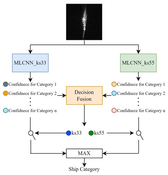
Figure 1. Architecture of LDF-D-MLCNNs.

3.1. Metaformer-like Convolutional Neural Networks

Our proposed SAR ship classification method comprises two MLCNNs with the same architecture, differing only in the kernel size of the depth-wise convolution layers. MLCNN_ks33 and MLCNN_ks55 use $(3,3)$ and $(5,5)$ as kernel sizes, respectively. The architecture of MLCNN is shown in Figure 2. The rectified linear unit (ReLU) [38] is used as activation, and batch normalization (BN) [39] is applied. Table 1 shows hyperparameters of MLCNN. Considering the application scenarios for ship classification, we constrained the computational complexity and model size of the MLCNN to be comparable to those of common small-sized computer vision models, such as ResNet-18 [29].

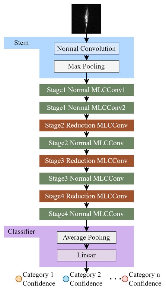
Figure 2. Architecture of MLCNN.

Table 1. Hyperparameters of MLCNN.

Module	Input Shape	Output Shape	Activation	Normalization	Channel Level Attention
Stem	$(1,100,100)$	$(64,25,25)$	ReLU	BN	None
Stage1 Normal MLCConv1	$(64,25,25)$	$(64,25,25)$	ReLU	BN	PSE
Stage1 Normal MLCConv2	$(64,25,25)$	$(64,25,25)$	ReLU	BN	PSE
Stage2 Reduction MLCConv	$(64,25,25)$	$(128,12,12)$	ReLU	BN	PSE
Stage2 Normal MLCConv	$(128,12,12)$	$(128,12,12)$	ReLU	BN	PSE
Stage3 Reduction MLCConv	$(128,12,12)$	$(256,6,6)$	ReLU	BN	PSE
Stage3 Normal MLCConv	$(256,6,6)$	$(256,6,6)$	ReLU	BN	PSE
Stage4 Reduction MLCConv	$(256,6,6)$	$(512,3,3)$	ReLU	BN	PSE
Stage4 Normal MLCConv	$(512,3,3)$	$(512,3,3)$	ReLU	BN	PSE
Classifier	$(512,3,3)$	n	SoftMax	None	None

An input SAR image is first processed by the stem, which comprises a standard convolution and max-pooling layer. The hyperparameters of our stem are shown in Table 2.

Table 2. Hyperparameters of stem.

Layer	Kernel Size	Input Shape	Output Shape	Activation	Normalization	Channel Level Attention
Normal Convolution	$(7,7)$	$(1,100,100)$	$(64,50,50)$	ReLU	BN	None
Max Pooling	$(3,3)$	$(64,50,50)$	$(64,25,25)$	None	None	None

The normal convolution layer is the most common layer in CNNs. Cross-correlation is computed between the kernel weights and the window pixels, slicing over the input. In the simplest case, the output value of the normal convolution layer can be precisely described as follows:

$$Conv(input)=\sum _{n=1}^{C}Weigh{t}_n^{Conv}\otimes inpu{t}_n$$

(1)

where C denotes a number of channels, and ⊗ is the valid 2D cross-correlation operator.

The outputs of the convolution layer are processed by BN before being activated. Applying BN adjusts the mean and variance of feature maps during training to mitigate internal covariate shifts, thereby improving training. The BN [39] can be calculated as follows:

$$BN\left(input\right)={\displaystyle \frac{input-Mean\left[input\right]}{\sqrt{Var\left[input\right]+ϵ}}} \times \gamma +\kappa$$

(2)

where $ϵ$ is a small number close to zero to prevent a zero denominator, and $\gamma$ and $\kappa$ are trainable parameters. $Mean$ denotes the mean operation and $Var$ denotes the variance operation, which are calculated per dimension over a mini-batch.

The backbone of MLCNN comprises eight MLCConv blocks, organized into four stages. The shape of the feature maps is reduced as we enter a new stage. Therefore, starting from the second stage, the reduction MLCConv blocks are interleaved with normal MLCConv blocks. Section 3.1.1 will introduce more details about our proposed MLCConvs.

The classifier of MLCNN is a sequential architecture comprising a global pooling layer and a linear layer, which is popular in computer vision [26,29,30]. This architecture can relieve overfitting caused by a large number of neurons and unified shapes of feature maps from different samples. The hyperparameters of our classifier are shown in Table 3.

Table 3. Hyperparameters of classifier.

Layer	Kernel Size	Input Shape	Output Shape	Activation	Normalization	Channel Level Attention
Average Pooling	$(3,3)$	$(512,3,3)$	512	None	None	None
Liner		512	n	SoftMax	None	None

3.1.1. Metaformer-like Compound Convolution Blocks

Inspired by the Metaformer concept, the MLCConv block is proposed in this paper. The architectures of both MLCConv block types are shown in Figure 3. An MLP is appended to 2 stacked MBConv sub-blocks. Following standard practices in computer vision, activation and normalization are applied after a convolutional layer. Similarly, reduction MLCConv blocks serve as learnable downsampling operations, reducing the feature map shape. For an input with a shape of $(c,h,w)$, the hyper-parameters of normal and reduction MLCConv blocks are shown in Table 4 and Table 5 respectively.

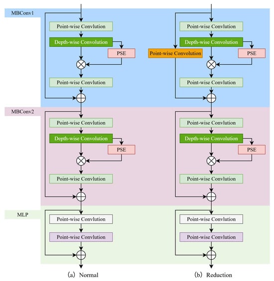
Figure 3. Architectures of MLCConv blocks.

Table 4. Hyperparameters of normal MLCConv block.

Sub-Block	Layer	Kernel Size	Input Shape	Output Shape	Activation
MBConv 1	Point-wise Convolution 1	$(1,1)$	$(c,h,w)$	$(2 \times c,h,w)$	ReLU
	Depth-wise Convolution	$(3,3)$ or $(5,5)$	$(2 \times c,h,w)$	$(2 \times c,h,w)$	ReLU
	PSE		$(2 \times c,h,w)$	$(2 \times c,h,w)$	ReLU
	Point-wise Convolution 2	$(1,1)$	$(2 \times c,h,w)$	$(c,h,w)$	None
MBConv 2	Point-wise Convolution 1	$(1,1)$	$(c,h,w)$	$(2 \times c,h,w)$	ReLU
	Depth-wise Convolution	$(3,3)$ or $(5,5)$	$(2 \times c,h,w)$	$(2 \times c,h,w)$	ReLU
	PSE		$(2 \times c,h,w)$	$(2 \times c,h,w)$	ReLU
	Point-wise Convolution 2	$(1,1)$	$(2 \times c,h,w)$	$(c,h,w)$	None
MLP	Point-wise Convolution 1	$(1,1)$	$(c,h,w)$	$(2 \times c,h,w)$	ReLU
	Depth-wise Convolution 2	$(1,1)$	$(2 \times c,h,w)$	$(c,h,w)$	None

Table 5. Hyperparameters of the reduction MLCConv block.

Sub-Block	Layer	Kernel Size	Input Shape	Output Shape	Activation
MBConv 1	Point-wise Convolution 1	$(1, 1)$	$(c, h, w)$	$(4 \times c,h,w)$	ReLU
	Depth-wise Convolution	$(3,3)$ or $(5,5)$	$(4 \times c,h,w)$	$(4 \times c,{\displaystyle \frac{h}{2}},{\displaystyle \frac{w}{2}})$	ReLU
	PSE		$(4 \times c,{\displaystyle \frac{h}{2}},{\displaystyle \frac{w}{2}})$	$(4 \times c,{\displaystyle \frac{h}{2}},{\displaystyle \frac{w}{2}})$	ReLU
	Point-wise Convolution 2	$(1,1)$	$(4 \times c,{\displaystyle \frac{h}{2}},{\displaystyle \frac{w}{2}})$	$(2 \times c,{\displaystyle \frac{h}{2}},{\displaystyle \frac{w}{2}})$	None
MBConv 2	Point-wise Convolution 1	$(1,1)$	$(2 \times c,{\displaystyle \frac{h}{2}},{\displaystyle \frac{w}{2}})$	$(4 \times c,{\displaystyle \frac{h}{2}},{\displaystyle \frac{w}{2}})$	ReLU
	Depth-wise Convolution	$(3,3)$ or $(5,5)$	$(4 \times c,{\displaystyle \frac{h}{2}},{\displaystyle \frac{w}{2}})$	$(4 \times c,{\displaystyle \frac{h}{2}},{\displaystyle \frac{w}{2}})$	ReLU
	PSE		$(4 \times c,{\displaystyle \frac{h}{2}},{\displaystyle \frac{w}{2}})$	$(4 \times c,{\displaystyle \frac{h}{2}},{\displaystyle \frac{w}{2}})$	ReLU
	Point-wise Convolution 2	$(1,1)$	$(4 \times c,{\displaystyle \frac{h}{2}},{\displaystyle \frac{w}{2}})$	$(2 \times c,{\displaystyle \frac{h}{2}},{\displaystyle \frac{w}{2}})$	None
MLP	Point-wise Convolution 1	$(1,1)$	$(2 \times c,{\displaystyle \frac{h}{2}},{\displaystyle \frac{w}{2}})$	$(4 \times c,{\displaystyle \frac{h}{2}},{\displaystyle \frac{w}{2}})$	ReLU
	Depth-wise Convolution 2	$(1,1)$	$(4 \times c,{\displaystyle \frac{h}{2}},{\displaystyle \frac{w}{2}})$	$(2 \times c,{\displaystyle \frac{h}{2}},{\displaystyle \frac{w}{2}})$	None

Feature maps fed into an MLCConv are initially processed by two stacked MBConv sub-blocks. We adopt the MBConv block variant from EfficientNet [26]. This version incorporates a residual connection and channel-level attention to achieve strong feature extraction with high efficiency. The number of channels of feature maps is increased by a point-wise convolution layer. Then, a depth-wise convolution layer further extracts some features, and new feature maps are calibrated by channel-level attention. Lastly, the other point-wise convolution layer reduces the number of channels of the feature maps to a pre-defined value.

A point-wise convolution layer is a normal convolution layer with a kernel size of $(1,1)$, and the depth-wise convolution layer only connects an input channel to a kernel. The equation of depth-wise convolution is shown below:

$$DWConv(inpu{t}_i)=Weigh{t}^{DWConv}\otimes inpu{t}_i$$

(3)

A block architecture with multiple low-computation layers is more efficient than a single convolutional layer. When the network width is low, the inverted bottleneck architecture enables MBConv to outperform the depth-wise separable convolution block in MobileNet [40]. MBConv remains a popular choice for low-complexity networks. Hence, the total computational complexity of MLCNN can be constrained to a level similar to that of small- to medium-sized computer vision networks, such as ResNet-18.

MLCConv is designed to process two-dimensional data, such as images. Hence, the MLP of MLCConv is implemented by stacking two point-wise convolution layers. Consequently, MLCConv can be considered a convolutional block.

The proposed MLCConv does not fully follow the Metaformer block. MBConv is a widely used convolutional module and provides excellent computational efficiency. Therefore, in our design concept, the architecture of MBConv is not intended to be modified. In the MBConv sub-block, normalization is performed after each convolutional layer. To ensure that the distributions of feature maps for the addition operation after the MLP are consistent, we apply normalization to the convolutional layers in the MLP. At the same time, each MBConv sub-block has its own residual connection, and there is no shortcut between the input and the second MBConv sub-block. Hence, the proposed MLCConv block shows differences from the Metaformer concept in the configuration of normalization and residual connection. Figure 4 illustrates these differences.

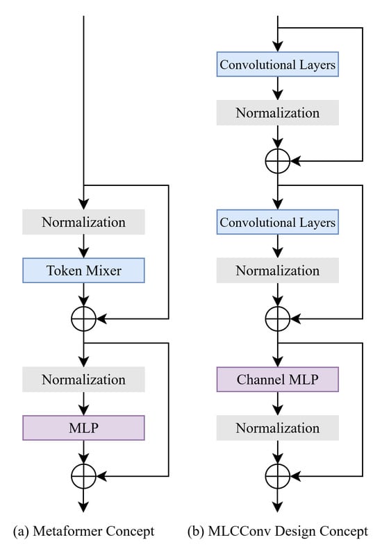
Figure 4. Comparisons between the Metaformer and MLCConv blocks.

3.1.2. Pyramid Squeeze and Excitation Module

The PSE module is designed based on the popular channel-level attention module SE [19] in this paper. In the PSE module, a weight to determine the importance of a channel is generated using multiple scales. Figure 5 shows the architecture of the PSE module. Three average pooling layers produce feature maps with the shape of $(C,4,4)$, $(C,2,2)$ and $(C,1,1)$ respectively. The output of each pooling layer is connected to a linear layer. Then, we concatenate the outputs of the linear layers and use the 4th linear layer to compute the channel importance weights. For an input with a shape of $(c,h,w)$, the hyperparameters of the PSE module are shown in Table 6.

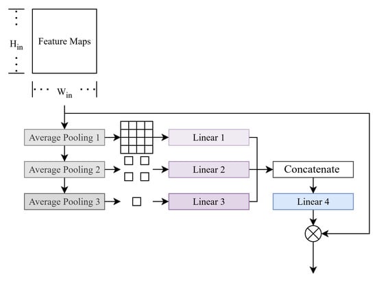
Figure 5. Architecture of the PSE module.

Table 6. Hyperparameters of the PSE module.

Layer	Kernel Size	Input Shape	Output Shape	Activation
Pooling 1	$({\displaystyle \frac{h}{4}},{\displaystyle \frac{w}{4}})$	$(c,h,w)$	$(c,4,4)$	None
Pooling 2	$(2,2)$	$(c,4,4)$	$(c,2,2)$	None
Pooling 3	$(2,2)$	$(c,2,2)$	$(c,1,1)$	None
Linear 1		$(c,4,4)$	${\displaystyle \frac{c}{16}}$	ReLU
Linear 2		$(c,2,2)$	${\displaystyle \frac{c}{16}}$	ReLU
Linear 3		$(c,1,1)$	${\displaystyle \frac{c}{16}}$	ReLU
Linear 4		${\displaystyle \frac{3 \times c}{16}}$	c	Sigmoid

The SE module uses global average pooling to downsample a feature map to one element and generate channel-wise weights that depend only on this global scale. However, targets, clutter, and speckle noise are not uniformly distributed in spatial dimensions. The global scale is insufficient to determine the importance of a channel. In computer vision, deep learning-based object detectors usually employ multiple scales to process the feature maps and assign different heads to further produce the detection box. Inspired by this design and considering efficiency, we modified the popular attention module, SE, to achieve channel-level attention across multiple scales.

Building upon the original SE block, our proposed PSE inherits its plug-and-play capability, allowing for seamless integration into MBConv. PSE can replace the original SE in MBConv and be deployed following the depth-wise convolutional layers. Also, our PSE has a high efficiency. PSE does not contain any convolutional operators and uses many weight-free operators. Although its computational complexity is slightly higher than that of the original SE, it remains significantly lower than that of many other computer vision attention modules.

3.2. Learnable Decision Fusion

The logits from two MLCNNs are concatenated and processed by the learnable decision fusion module to obtain the final prediction. With this design, MLCNNs can co-operate to utilize their advantages on different types of features. Compared with other level fusion and network architecture search methods, decision fusion is simpler and requires fewer training samples. Hence, decision fusion is applied to the SAR ship classification dataset, which contains low-quality images and limited samples. In addition, decision fusion shows an advantage in robustness. When a branch or dataflow fails, the classification can also be operated with an acceptable performance.

The learnable decision fusion module in this paper is an MLP activated by Gaussian error linear unit (GELU) [41]. The hyper-parameters of the learnable decision fusion module are listed in Table 7.

Table 7. Hyperparameters of the learnable decision fusion module.

Sub-Module	Layer	Input Shape	Output Shape	Activation
Embedding	Linear	$2 \times$ Number of Categories	512	GELU
MLP	Linear 1	512	512	GELU
	Linear 2	512	1	Sigmoid

Usually, weight-free decision methods are based on simple operators, such as voting, max, and average. However, fusion for MLCNNs is more difficult. Each MLCNN used can be considered a set of weights trained via gradient descent. The performance gap between both MLCNNs is very small. It is difficult to apply weight-free decision fusion methods in this situation. Hence, this paper employs a learnable architecture trained following the training script of deep neural networks to obtain a better fusion performance.

Two group confidence values for all categories can be obtained by feeding SAR images to MLCNNs. Our decision fusion module takes the concatenated logits as input and produces a value to determine which MLCNN is more likely to produce the correct prediction. If the value is smaller than $0.5$, the output from the MLCNN with the kernel size of $(3,3)$ will be set as the final prediction. Otherwise, the output from the MLCNN with the kernel of $(5,5)$ will be the final prediction of our proposed classification method.

To increase learning capacity and introduce greater nonlinearity, the MLP in the decision fusion module adopts an inverted bottleneck architecture and is activated with GELU. This design is popular in modern MLP-based architectures, such as Transformer encoders. GELU is a popular non-linear activation function and has good smoothness and stability. The equation of GELU is shown below:

$$GELU(x)=x \times \Phi (x)$$

(4)

where $\Phi (x)$ is the cumulative distribution function of Gaussian distribution.

We use a pseudo-label to train the weights in the decision fusion module, rather than directly using the labels corresponding to the samples. The number of samples in a SAR ship dataset is usually very small. Deep learning models frequently suffer from severe overfitting. Even when applying a large number of anti-overfitting tricks, the performance between training and test sets remains significant. Both MLCNNs can achieve very high accuracy on the training set, and it is very difficult to use the true labels to train a decision fusion module that effectively distinguishes between the two MLCNNs. To enlarge the gap between the performance of both MLCNNS, we set the pseudo label of a sample as the MLCNN that achieves a lower cross-entropy loss. Hence, as a binary classification task, the MLP has a single output neuron activated by the sigmoid function to output the prediction. In addition, a stronger data augmentation policy is applied during training of the decision fusion model to make the logits from MLCNNs contain more noise, which improves the learning.

4. Ship Classification Experiments Setup

To verify the effectiveness of the proposed method, experiments were conducted on a workstation equipped with an Intel Core i5-11600 CPU. Training was performed using a single NVIDIA RTX 3060 GPU. The proposed method is developed using PyTorch (torch 2.0.1+cu117) [42], which is a popular deep learning framework. We utilized an open-source tool [43] to calculate the computational complexity and model size.

4.1. Datasets

This paper focuses on improving ship classification accuracy using low-quality SAR images. Experiments utilize both real-world measured data and simulated samples under jamming situations.

4.1.1. Actual SAR Images

OpenSARShip and FUSARShip, which are popular in SAR ship classification research, were used. All samples in them are collected from actual radars.

OpenSARShip is an open-access dataset containing 11,346 SAR images in ground range detected and single look complex mode [44]. The labels are generated by the related ship information from AIS. However, the sample numbers of categories are highly imbalanced. Referring to published SAR ship classification research, the single-look complex samples of bulk carriers, container ships, and tankers are selected to build a classification task [15]. Those 3 categories of ship account for approximately $80\%$ of the share in international shipping [45]. The single-look complex products provide both VV and VH polarizations for a target with good range resolution. To avoid the long-tail problem during training, we follow the same approach described in the published literature. The lowest target number across all three categories is used as the uniform target count for each category. The remainder of the targets are used for testing. To prevent data leakage, the VV and VH images of the same target are treated as two distinct samples and assigned exclusively to the same data split. If the VH image of a target is used for training, the VV image of this target must be used for training too. Some samples from OpenSARShip are shown in Figure 6. The number of instances for each classification category based on OpenSARShip is shown in Table 8.

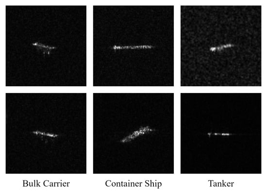
Figure 6. SAR ship samples in the classification task based on OpenSARShip.

Table 8. Sample numbers of each category in the classification task based on OpenSARShip.

Category	Total Sample	Training Sample	Test Sample
Bulk Carrier	666	338	328
Container Ship	1146	338	808
Tanker	484	338	146

FUSARShip is another widely used open-access SAR ship dataset [13]. All samples in FUSARShip are collected from Gaofen-3 civil C-band fully polarimetric spaceborne SAR. The labels are also from the shipborne AIS. In addition to maritime targets, FUSARship contains samples of non-ship targets, land, clutter, and false alarms. Although this dataset contains a large number of samples, the category imbalance is significantly more severe. Four common categories of civil ships, bulk carriers, fishing ships, cargoes, and tankers, are selected to construct a classification task containing both inshore and offshore scenarios. Similarly, $70\%$ of the smallest sample size in all four categories is set as the uniform number of training targets for each category. Moreover, some categories have significantly more samples than other categories, which biases the test results towards dominant categories. Hence, the testing sample number of each category is configured to be the third largest number of remainder samples in the involved categories. Some samples from FUSARShip are shown in Figure 7. The number of each category of the classification task based on FUSARShip is shown in Table 9.

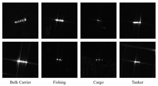
Figure 7. SAR ship samples in the classification task based on FUSARShip.

Table 9. Sample numbers of each category in the classification task based on FUSARShip.

Category	Total Sample	Training Sample	Test Sample
Bulk Carrier	274	174	100
Fishing	787	174	100
Cargo	1735	174	100
Tanker	248	174	74

4.1.2. Simulated SAR Images Under Jamming Situations

The simulated SAR ship images under jamming situations in this paper were generated by Feko (2021.1) and MATLAB (R2024a).

Five different ship 3D models were included. The radar was configured as a waveform, linear frequency modulation; pulse width, $0.24$ µs; sampling rate, 140 MHz. Three types of jamming signals were simulated, including noise frequency modulation, sweep frequency, and dense false target jamming.

Noise-frequency modulation jamming is a type of barrage jamming and can produce signals with large bandwidths. Noise-frequency modulation is widely used because it requires minimal precise measurement of the radar carrier frequency. The equation for noise frequency modulation jamming signal is given below:

$$J_{nfm}(t)=A_{nfm}exp\left(j2\pi f_{j}t+2\pi K_{nfm}{\int }_0^t{U}_n\left(t\right)dt\right)$$

(5)

where A is the jamming signal amplitude; $f_j$ is the jamming carrier frequency; and $U_n\left(t\right)$ is a Gaussian noise with zero mean and ${\sigma }^2$ variance.

Sweep-frequency jamming can be generated by periodically performing a narrowband noise scan at the radar’s potential carrier frequency. The equation for the sweep frequency jamming signal is given below:

$$J_{sf}=A_{sf}exp{\displaystyle \left(j2\pi f_{sf}\left(t\right)t\right)}{U}_{sf}\left(t\right)$$

(6)

where $f_{sf}(t)$ is a frequency modulation function, and $U_{sf}(t)$ represents narrowband noise.

Dense false-target jamming has become popular following the development of digital radio-frequency memory. The jammer captures the radar signals. Subsequently, a large number of false target signals can be transmitted by modulating the range and Doppler information of the captured radar signals. False targets can corrupt the geometric information of the true target in processed SAR images. The equation for dense false target jamming signal is given below:

$$J_{dft}\left(t\right)=\sum _m^M{A}_{dft}^{m}S{\displaystyle \left(t-{\tau }_{dft}^m\right)}exp{\displaystyle \left(j2\pi {fd}_{dft}^m\right)}$$

(7)

where $S(t)$ is radar signal; $\tau$ is a range modulation; and d is a Doppler modulation.

To build the ship dataset under jamming conditions for training the proposed method in this paper, we first used professional electromagnetic simulation software to compute the radar cross sections (RCS) of ships and the sea surface from 3D models. A linear frequency-modulated pulse signal, a common waveform used in SAR, is employed to obtain the target’s time-domain echo based on simulated RCS results and predefined angles. The jamming-to-signal ratio in our simulation ranged from 0 dB to 20 dB, and the step size was 5 dB. The main configuration of the involved jamming is shown in Table 10. Then, jamming signals were generated following Equations (5)–(7). Usually, the echoes from the ship reflection and jamming signals sent by jammers are mixed in space before entering the radar receiver antenna. Hence, in the simulation experiments of this paper, the jamming for each sample is mixed with the target echo in the time domain to simulate the actual engineering scenario. Some samples are shown in Figure 8 to demonstrate the effect of different jamming. Noise frequency modulation and sweep frequency jamming, as types of suppression jamming, are unable to obtain the gain produced in the SAR imaging stage. Hence, those jamming patterns could not be condensed into points. Therefore, they form a fog-like result that hinders further awareness of SAR images. On the other hand, dense false target jamming is a type of deception jamming that generates signals highly similar to the ship’s echo. This jamming can fully enjoy the gain of the expected signal in the SAR imaging algorithm. As a result, it presents as small, high-brightness white spots in the final SAR samples. The energy of dense false target jamming is concentrated, which makes the brightness of the ship in the SAR image close to the background and reduces the effectiveness of the work of following awareness algorithms.

Table 10. Configuration of jamming in simulation.

Jamming Type	Total Sample
Noise frequency modulation	Bandwidth: 60–120 MHz
Sweep frequency	Noise bandwidth: 5–20 MHz
	Frequency range: 60–120 Mhz
	Sweep frequency: $1.25$–$2.5$ Mhz
Dense false targets	Number of false target: 15–25
	Range unit modulation: −100–100
	Azimuth unit modulation: −100–100

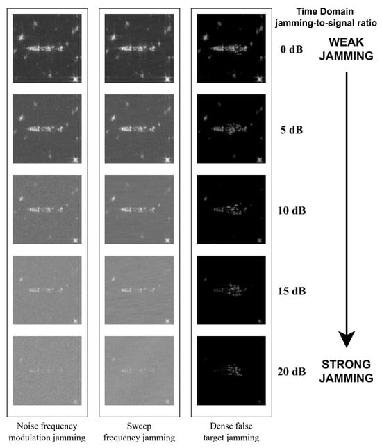
Figure 8. Simulated SAR images of a target under different jamming situations.

The azimuth angle in the simulation was from 0 to 355 degrees, and the step size was 5 degrees. Some samples with different azimuth angles are shown in Figure 9. Two elevation angles were simulated, where samples at 30 degrees were used for training and 35 degrees were used for testing. Hence, the classification task based on the simulation under jamming situations contains 5400 samples for training and the other 5400 samples for testing.

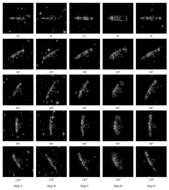
Figure 9. SAR ship samples in classification task based on simulation.

4.2. Training

The training of the proposed SAR-based ship classification method comprises three stages. In the first stage, only the MLCNN with $(3,3)$ kernel size was trained; and in the second stage, only the MLCNN with $(5,5)$ kernel size was trained. The same training script was used for those two stages. Finally, the weights of the trained MLCNNs were frozen, and only the decision fusion module was trained in the third stage with a more aggressive data augmentation policy.

Because they are trained on classification tasks, MLCNNs use cross-entropy loss. We define fusion as a classification task with only two categories in the proposed method. Therefore, the decision fusion module uses binary cross-entropy loss. The configuration of the optimizer remained consistent across all stages. The training for each stage lasted for 600 epochs, and each batch contained 96 samples. The stochastic gradient descent optimizer was employed to update the weights of the neural network. The initial and final learning rates were set as $0.0025$ and 0, respectively. During training, the cosine annealing scheduler adjusted the learning rate based on the following equation:

$${\eta }_{current}={\eta }_{min}+{\displaystyle \frac{1}{2}}({\eta }_{max}-{\eta }_{min})(1+cos({\displaystyle \frac{Epoc{h}_{current}}{Epoc{h}_{final}}}))$$

(8)

where ${\eta }_{current}$, ${\eta }_{min}$, and ${\eta }_{max}$ are the current, initial, and final learning rates, respectively. $Epoc{h}_{current}$ and $Epoc{h}_{final}$ represent the current epoch index and the total number of epochs, respectively.

The data augmentation policy was kept the same in the first and second stages, including random cropping, cutout [46], and random horizontal flipping. To further widen the performance gap between MLCNNs, a stronger data augmentation policy was employed in the third stage. In addition to the transformation methods used in the previous stages, random vertical flipping and pepper noise were applied.

4.3. Evaluation Metrics

Following similar studies [15,21,25,27], we use accuracy, recall, precision, and F1 as performance metrics. Following prior work on lightweight networks in computer vision, we also use multiply-accumulate operations and the number of weights to evaluate model computational complexity and size, respectively.

Accuracy is the most important metric for classification tasks and is used in both optical and SAR image classification. Accuracy can be calculated as follows:

$$\begin{array}{c}\hfill Accuracy={\displaystyle \frac{TP+TN}{TP+TN+FP+FN}}\end{array}$$

(9)

where $TP$, $TN$, $FN$, and $TN$ denote the number of true positives, false positives, false negatives, and true negatives, respectively.

Recall quantifies the proportion of actual positives that are correctly identified, focusing on minimizing false negatives. Recall can be calculated as follows:

$$Recall={\displaystyle \frac{TP}{TP+FN}}$$

(10)

Precision measures the proportion of positive predictions that are correctly identified and can be calculated as follows:

$$Precision={\displaystyle \frac{TP}{TP+FP}}$$

(11)

The F1 score provides a single metric to balance the trade-off between recall and precision. The equation for the F1 score is defined as follows:

$$F1=2 \times {\displaystyle \frac{Recall \times Precision}{Recall+Precision}}$$

(12)

Multiply-accumulate operations are fundamental to the functioning of neural networks. Each Multiply-accumulate operation contains a multiplication followed by an addition. The number of multiply and accumulate operations is usually considered as a measure of computational complexity and can be counted automatically by software [43].

As a learnable algorithm, a neural network contains many weights. Counting the number of weights, including both learnable and fixed, directly reflects a network’s storage usage. In this paper, the number of weights in a network was automatically obtained by software [43].

5. Performance Results and Analysis

5.1. Compared with Deep Learning-Based SAR Ship Classification Methods

To evaluate the performance of the proposed method, we selected nine published deep learning-based SAR ship classification methods for comparison: the VGGNet based on transfer learning (TL-VGGNet) [11], GSESCNN [12], HOG-ShipCLSNet [15], VGGNet with hybrid channel feature loss (HCLF-VGGNet) [47], mini hourglass region extraction and dual-channel efficient fusion network (RE-DC-EfficientNet) [22], SE-LPN-DPFF [25], polarization fusion network with geometric feature embedding (PFGFE-Net) [21], DPIG-Net [14], and feature joint learning (FJL) framework [27]. The three-category classification task based on the OpenSARShip dataset has become widely accepted by related research and can now serve as a benchmark. The results of the comparative methods are taken from publicly available publications. This is to avoid potential discrepancies caused by differences in implementation details, such as software versions or random seeds.

The results of the ship classification task based on OpenSARShip are shown in Table 11. The proposed method achieves the highest accuracy and outperforms other listed deep learning-based SAR ship classification methods. The proposed MLCNN has a strong learning capability. The fusion of two MLCNNs with different kernel sizes can more effectively process samples that are challenging for a single network.

Table 11. Comparison with SAR ship classification methods on the classification task based on OpenSARShip.

Method	Accuracy	Recall	Precision	F1
TL-VGGNet [11]	$69.27\%$	$57.75\%$	$58.72\%$	$58.12\%$
GSESCNN [12]	$74.98\%$	$74.74\%$	$69.56\%$	$72.04\%$
HOG-ShipCLSNet [15]	$78.15\%$	$77.87\%$	$72.42\%$	$75.05\%$
HCLF-VGGNet [47]	$77.41\%$	$74.99\%$	$74.25\%$	$74.52\%$
RE-DC-EfficientNet [22]	$75.44\%$	$73.87\%$	$71.50\%$	$72.67\%$
SE-LPN-DPFF [25]	$79.25\%$	$78.83\%$	$76.45\%$	$77.62\%$
PFGFE-Net [21]	$79.84\%$	—	—	$78.00\%$
FJL framework [27]	$79.02\%$	$78.38\%$	$73.97\%$	—
DPIG-Net [14]	$81.28\%$	—	—	—
LDF-D-MLCNNs (Ours)	$82.45\%$	$81.99\%$	$78.57\%$	$80.06\%$

In terms of computational complexity, the proposed network is designed to match the scale of small- to medium-sized general computer vision classification networks and requires $757.57$ million multiply–add operations per inference. This is comparable to ResNet-34. Meanwhile, most computations occur within neural network layers, making the proposed method well-suited for acceleration on neural processing units. Some methods listed in Table 11 require additional polarization information or rely on traditional mathematical feature extraction, such as principal components analysis. After a decade of development, specialized neural inference devices on embedded platforms can support the computational budget of medium-sized networks. Therefore, we believe our method achieves a good trade-off among performance, convenience, and application prospects.

Table 12 shows the confusion matrix of the proposed method on the classification task based on OpenSARShip. Most of the samples were predicted correctly. The main source of confusion is between the bulk carrier and container ship categories, a pattern observed in other deep learning-based SAR ship classification methods. Those 2 categories of ships are very similar in shape, and the quality of the samples is relatively poor.

Table 12. Confusion matrix of proposed method on task based on OpenSARShip.

	Bulk Carrier	Container Ship	Tanker
Bulk Carrier	$71.04\%$	$25.61\%$	$3.35\%$
Container Ship	$10.02\%$	$85.89\%$	$4.08\%$
Tanker	$3.42\%$	$7.53\%$	$89.04\%$

5.2. Compared with Computer Vision Networks

To further verify the effectiveness of the proposed method, ten popular computer vision networks are compared on classification tasks using OpenSARShip and FUSARShip. Half of the involved networks are small to medium size, including ResNet-34 [29], EfficientNet-b6 [26], DenseNet-121 [48], ViT-small [17], and ConvNext-Tiny [31]. The remaining five small-sized networks are ResNet-18 [29], EfficientNet-b0 [26], MobileNet v2 [30], ViT-tiny [17], and CCT-722 [36]. The codes for all compared methods are sourced from open-source projects. To ensure a fair comparison, both the proposed method and the computer vision models were trained using an identical script, which fixed the random seed and optimizer settings. All training was conducted under the same software environment on a single machine. We performed one independent training run for each method on each of the two classification tasks.

Table 13 shows the comparison of the proposed method and some popular computer vision networks in classification based on OpenSARShip. The results indicate that computer vision networks can achieve good performance on SAR ship classification. The proposed method achieves the highest accuracy and has computational complexity comparable to that of small- to medium-sized computer vision networks. In addition, the number of training samples for SAR ship classifications is lower than that of common optical object classification datasets, such as Cifar-10 and ImageNet. Hence, the low generalization capability problem of the Transformer becomes more serious, which leads Transformer-based networks to demonstrate lower performance than CNNs in the comparison. Also, in some network architectures, smaller versions have better performance. We attribute this to the limited number and poor quality of training samples, which exacerbates overfitting in those larger versions.

Table 13. Comparison with computer vision networks on a task based on OpenSARShip.

Method	Accuracy	Multiply-Accumulate Operations	Weights
ResNet-34 [29]	$78.31\%$	$897.00$ M	$21.29$ M
EfficientNet-b6 [26]	$79.56\%$	$904.90$ M	$40.52$ M
ViT-Small [17]	$64.59\%$	$809.33$ M	$56.95$ M
DenseNet-121 [48]	$78.08\%$	$904.90$ M	$6.87$ M
ConvNext-Tiny [31]	$64.98\%$	$829.99$ M	$27.80$ M
ResNet-18 [29]	$79.79\%$	$443.40$ M	$11.18$ M
EfficientNet-b0 [26]	$77.06\%$	$100.68$ M	$3.97$ M
ViT-Tiny [17]	$64.35\%$	$208.26$ M	$5.49$ M
MobileNetv2 [30]	$77.14\%$	$75.45$ M	$2.19$ M
CCT-772 [36]	$75.66\%$	$274.07$ M	$4.51$ M
LDF-D-MLCNNs (Ours)	$82.45\%$	$757.57$ M	$33.71$ M

Table 14 shows the comparison of the proposed method and some popular computer vision networks in classification based on FUSARShip. The proposed method also shows an advantage in accuracy. This classification task includes single-target scenarios and scenarios in which the target is surrounded by unrelated ships, and the number of training samples is lower. Hence, the difficulty of the classification task based on FUSARShip is higher. The proposed method and the listed computer vision networks all have decreased performance.

Table 14. Comparison with computer vision networks on task based on FUSARShip.

Method	Accuracy	Multiply-Accumulate Operations	Weights
ResNet-34 [29]	$63.10\%$	$897.00$ M	$21.29$ M
EfficientNet-b6 [26]	$63.36\%$	$904.90$ M	$40.52$ M
ViT-Small [17]	$56.95\%$	$809.33$ M	$56.95$ M
DenseNet-121 [48]	$64.82\%$	$904.90$ M	$6.87$ M
ConvNext-Tiny [31]	$59.09\%$	$829.99$ M	$27.80$ M
ResNet-18 [29]	$60.16\%$	$443.40$ M	$11.18$ M
EfficientNet-b0 [26]	$61.49\%$	$100.68$ M	$3.97$ M
ViT-Tiny [17]	$58.29\%$	$208.26$ M	$5.49$ M
MobileNetv2 [30]	$60.43\%$	$75.45$ M	$2.19$ M
CCT-772 [36]	$57.75\%$	$274.07$ M	$4.51$ M
LDF-D-MLCNNs (Ours)	$65.24\%$	$757.57$ M	$33.71$ M

Table 15 details the class-wise performance of the proposed method on the classification task based on FUSARShip. Most bulk carriers, fishing vessels, and cargo samples can be classified correctly. The accuracy of liquid cargo is low. The tanker category in FUSARShip comprises several subcategories, including oil product tankers, liquefied gas tankers, and crude oil tankers. The differences between those subcategories are significant. The sample size of the tanker category is also smaller than that of other categories. However, the proposed method does not explicitly address intra-class variability in a category and the long tail problem. Thus, the network focuses on reducing the loss from the categories with lower learning difficulty and has a relatively lower accuracy for the tanker category.

Table 15. Confusion matrix of proposed method on task based on FUSARShip.

	Bulk Carrier	Fishing	Cargo	Tanker
Bulk Carrier	$79\%$	$12\%$	$2\%$	$7\%$
Fishing	$8\%$	$64\%$	$11\%$	$17\%$
Cargo	$1\%$	$7\%$	$69\%$	$23\%$
Tanker	$21\%$	$28\%$	$8\%$	$43\%$

5.3. Ship Classification Under Jamming Situations

Jamming can degrade the quality of SAR images and increase the classification difficulty. To further validate the robustness and effectiveness of the proposed algorithm, we conducted additional experiments on the classification task based on the simulation containing three jamming types. Using the same training script, both the proposed algorithm and the general computer vision models compared in Section 5.2 were each trained independently for one run.

Table 16 shows the comparison of the proposed method and some popular computer vision networks on the classification based on the simulation. The experimental results show that small- to medium-sized networks achieve better performance than small-sized networks. Classifying jammed SAR images requires models with higher learning capacity. The proposed LDF-D-MLCNNs achieves the best accuracy, outperforming popular computer vision networks. MLCNNs in the proposed method complement each other, enabling more effective utilization of the remaining features in jammed SAR images.

Table 16. Comparison with computer vision networks on a classification task based on simulation.

Method	Accuracy	Multiply-Accumulate Operations	Weights
ResNet-34 [29]	$93.57\%$	$897.00$ M	$21.29$ M
EfficientNet-b6 [26]	$93.44\%$	$904.90$ M	$40.52$ M
ViT-Small [17]	$72.94\%$	$809.33$ M	$56.95$ M
DenseNet-121 [48]	$92.89\%$	$904.90$ M	$6.87$ M
ConvNext-Tiny [31]	$76.63\%$	$829.99$ M	$27.80$ M
ResNet-18 [29]	$93.46\%$	$443.40$ M	$11.18$ M
EfficientNet-b0 [26]	$92.52\%$	$100.68$ M	$3.97$ M
ViT-Tiny [17]	$67.44\%$	$208.26$ M	$5.49$ M
MobileNetv2 [30]	$90.65\%$	$75.45$ M	$2.19$ M
CCT-772 [36]	$88.70\%$	$274.07$ M	$4.51$ M
LDF-D-MLCNNs (Ours)	$94.35\%$	$757.57$ M	$33.71$ M

Figure 10 shows the curve of accuracy under different jamming-to-signal ratios. The proposed method has good robustness and successfully maintains the performance under jamming situations ranging from 0 dB to 10 dB. Then, the accuracy is slightly decreased with the 15 dB jamming situation, but still at a high level. When the jamming situation reaches 20 dB, the meaningful information of a SAR image is significantly diminished, and human observers are unable to perform ship classification. Although the accuracy of the proposed method has been decreased by $10\%$, a larger proportion of targets can still be correctly classified. The proposed method can perform ship classification using SAR images under a certain level of jamming.

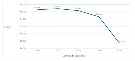
Figure 10. Classification accuracy of LDF-D-MLCNNs versus jamming-to-signal ratio.

5.4. Ablation Study

To verify the effectiveness of each modification in the proposed method, a series of ablation studies has been conducted on the classification task based on OpenSARShip. All the variant networks for comparison were trained with the same script as the proposed method.

5.4.1. MLCConv Block

To verify the increase in performance by appending an MLP to two stacked MBConv sub-blocks, the networks without MLP were trained. Also, the decision fusion module was trained from scratch. Table 17 shows the comparison of this ablation study. By appending MLPs, the performance has been increased. Research on Metaformer reveals that MLPs exhibit good flexibility and can be combined with many other components to enhance learning capacity. Due to the architecture of the MBConv sub-block, it is difficult to build a strict Metaformer with the MBConv sub-block. However, the performance of the MBConv-based CNN has been improved with MLPs.

Table 17. Comparison of whether to append MLP.

Convolutional Block	Accuracy
MLCConv	$82.45\%$
2 Stacked MBConv [26]	$80.57\%$

5.4.2. PSE Module

To verify the benefits of our modified channel-level attention module (PSE), we implemented MLCNNs equipped with the original SE module for comparison. Table 18 shows the results of this ablation study. Determining channel importance using multiple scales proves more effective than relying on a single global element.

Table 18. Comparison of different channel-level attention modules.

Channel Level Attention Module	Accuracy
PSE	$82.45\%$
SE [19]	$81.04\%$

5.4.3. Decision Fusion with MLCNNs of Different Kernel Size

To verify the effectiveness of decision fusion with MLCNNs of different kernel sizes, the performance of each individual MLCNN was evaluated. Both MLCNNs in the proposed method can operate independently to perform ship classification. Consequently, even if one MLCNN fails, the proposed method can still maintain an acceptable level of performance. Table 19 shows the accuracy of MLCNNs working independently. A single MLCNN can achieve good performance and outperform many computer vision networks. The MLCNN with a kernel size of $(3,3)$ has a better accuracy. Meanwhile, decision fusion further improves the performance, which means the proposed method can effectively enable the MLCNNs to complement each other.

Table 19. Comparison between independent MLCNNs and decision fusion.

Method	Accuracy
LDF-D-MLCNNs	$82.45\%$
MLCNN_ks33	$81.35\%$
MLCNN_ks55	$80.50\%$

To further verify the effectiveness of our decision fusion module, we have tested several other common fusion approaches. First, two common weight-free fusion methods, maximum and summation, were directly substituted for the proposed decision-level fusion module. Voting is not applicable in our system because only two experts are employed. Additionally, a learnable fusion module using the same architecture was trained using ground-truth labels. Comparative results are presented in Table 20. Learnable modules and summation fusion improve performance compared with individual networks. The learnable fusion outperforms weight-free methods. Furthermore, the proposed pseudo-label-based learnable fusion module achieves better results than the module trained with ground-truth labels. Training with pseudo-labels allows the micro-sized module to effectively perceive the advantages of different sub-networks on various samples.

Table 20. Comparison between different fusion policies.

Fusion Policy	Accuracy
Pseudo-label-based learnable module	$82.45\%$
Ground truth label-based learnable module	$81.75\%$
Maximum	$81.43\%$
Summation	$81.04\%$

Network scaling is commonly employed in computer vision to improve performance within a certain range at the cost of increasing computational complexity. To further present the value of our proposed decision fusion, we tested doubling the width of a single MLCNN and further doubling its depth. Table 21 shows that those scaled networks have decreased performance compared to the original single network. Obviously, the enlarged networks require more computational budgets. The proposed decision fusion policy uses a simple approach to further improve the performance of MLCNN.

Table 21. Comparison between decision fusion and network scaling.

Policy for Increasing Complexity	Accuracy
Fusion	$82.45\%$
2 × Width	$79.88\%$
2 × Depth	$79.49\%$
2 × Width & 2 × Depth	$80.27\%$

6. Discussion

6.1. Efficiency

We planned to make MLCNN have computational complexity comparable to that of ResNet-18. However, there are dual MLCNNs in our proposed method, and the complete computational complexity has been increased to the ResNet-34 level. Benefiting from the architecture with dual networks, the proposed method offers greater flexibility in practical applications and provides users with more options. If the platform has sufficient computational budget, the proposed method can achieve the expected performance and fully exploit hardware capabilities. Nowadays, embedded devices have become more important in markets. Numerous NPU platforms with continuously improving computational capabilities are presented, such as the Huawei Ascend A310 and Rockchip RK3588. Also, on platforms with limited computational resources, our method can still yield acceptable performance with only half the computational complexity. Moreover, our dual-network design can readily adopt a dynamic inference mechanism, allowing the computational complexity to be controlled at any level between using only a single network and full inference. For example, the simplest weight-free dynamic inference approach can be operated by assigning a random number between 0 and 1 to each input sample. If the value is below a certain threshold, only one network will be used. This provides greater flexibility for practical applications and better accommodates dynamic resource management, such as heat dissipation and power consumption.

To further improve efficiency, we will work on the dynamic network mechanism further [49,50]. First, we plan to append a router module to the initial layers of the first sub-network. This module will determine whether to continue inference in the first network or exit early to the second network. Second, we plan to make use of the distinct characteristics of SAR ship images, such as non-overlapping targets and simple backgrounds. Specialized networks for various interference conditions will be built and trained independently. A jamming situation awareness module can act as a router to select the appropriate network, thereby avoiding requiring a single network to learn backgrounds across all jamming types. Hence, the learning capability can be reduced, which means further lightweighting for the network will become possible.

6.2. Intra-Class Variations

In the experiment on the FUSARShip dataset, the proposed method achieved good overall performance. However, it achieved lower accuracy for the Tanker category than for the other categories. In this task, the specific ship instances within the Tanker category have differences in purpose and manufacturing process. This result forces us to confront intra-class variations arising from traditional ship category definition and modern shipbuilding developments. For example, USS Nicholas (DD-449) and USS Zumwalt (DDG-1000) both belong to the destroyer category. But their construction dates differ by nearly three-quarters of a century, leading to significant disparities in both optical and SAR images.

To address this practical issue, we plan to start with an actual engineering background in the future. During training, we will use pseudo-labels to split samples that exhibit large within-category variability into several subcategories. At the final output stage, these subcategories will be integrated into a single category. Pseudo-labels can be generated using AIS data from ships. Alternatively, sample matching scores can be computed using mathematical methods and grouped into several subcategories. Unsupervised learning can also be employed for clustering to obtain pseudo-labels [51]. Additionally, we will consider employing techniques from fine-grained image classification to enhance network performance, such as metric learning [52] and a local detail features module [53].

6.3. Few-Shot and Long Tail

This paper focuses on the network architecture. Due to time constraints, we did not extensively explore advanced training strategies. However, in some application scenarios, the number of available samples may be much smaller. Also, the sample numbers of categories in actual radar datasets are distributed in a large range. Many samples from the majority classes must be discarded to mitigate the long-tail problem.

To improve performance in extreme scenarios, we plan to jointly optimize training samples and the learning policy. A SAR image generator, such as a generative adversarial network [54] or diffusion model [55], will be used to enrich the samples for each category. Also, some learning policies, such as meta-learning [56] or auxiliary-task learning [57], enable currently unused data to contribute to the training process.

7. Conclusions

In this paper, a SAR ship classification method based on decision fusion and CNN, LDF-D-MLCNNs, is proposed. To improve feature extraction, the MLCConv block and the PSE module were designed within the MLCNN. Two different kernel sizes are used for depth-wise convolution layers in MLCNNs. The final prediction can be obtained by feeding the MLCNN logits into the proposed learnable decision fusion. Experimental results show that the proposed method achieves good performance in ship classification using real SAR images. In addition, the accuracy of the proposed method can be kept in an acceptable range under jamming situations.

References

- Yu, J.; Wang, Z.; Vasudevan, V.; Yeung, L.; Seyedhosseini, M.; Wu, Y. Coca: Contrastive captioners are image-text foundation models. arXiv 2022, arXiv:2205.01917. [Google Scholar]
- Wortsman, M.; Ilharco, G.; Gadre, S.Y.; Roelofs, R.; Gontijo-Lopes, R.; Morcos, A.S.; Namkoong, H.; Farhadi, A.; Carmon, Y.; Kornblith, S.; et al. Model soups: Averaging weights of multiple fine-tuned models improves accuracy without increasing inference time. In Proceedings of the International Conference on Machine Learning, PMLR, 2022, Baltimore, MD, USA, 17–23 July 2022; pp. 23965–23998. [Google Scholar]
- Chen, X.; Wang, X.; Changpinyo, S.; Piergiovanni, A.; Padlewski, P.; Salz, D.; Goodman, S.; Grycner, A.; Mustafa, B.; Beyer, L.; et al. Pali: A jointly-scaled multilingual language-image model. arXiv 2022, arXiv:2209.06794. [Google Scholar]
- Petit, M.; Stretta, J.M.; Farrugio, H.; Wadsworth, A. Synthetic aperture radar imaging of sea surface life and fishing activities. IEEE Trans. Geosci. Remote Sens. 1992, 30, 1085–1089. [Google Scholar] [CrossRef]
- Park, J.; Lee, J.; Seto, K.; Hochberg, T.; Wong, B.A.; Miller, N.A.; Takasaki, K.; Kubota, H.; Oozeki, Y.; Doshi, S.; et al. Illuminating dark fishing fleets in North Korea. Sci. Adv. 2020, 6, eabb1197. [Google Scholar] [CrossRef]
- Moreira, A.; Prats-Iraola, P.; Younis, M.; Krieger, G.; Hajnsek, I.; Papathanassiou, K.P. A tutorial on synthetic aperture radar. IEEE Geosci. Remote Sens. Mag. 2013, 1, 6–43. [Google Scholar] [CrossRef]
- Singh, P.; Shree, R.; Diwakar, M. A new SAR image despeckling using correlation based fusion and method noise thresholding. J. King Saud Univ.-Comput. Inf. Sci. 2021, 33, 313–328. [Google Scholar] [CrossRef]
- Singh, P.; Shankar, A.; Diwakar, M. Review on nontraditional perspectives of synthetic aperture radar image despeckling. J. Electron. Imaging 2023, 32, 021609. [Google Scholar] [CrossRef]
- Alex, K. Learning Multiple Layers of Features from Tiny Images; University of Toronto: Toronto, ON, USA, 2009. [Google Scholar]
- Deng, J.; Dong, W.; Socher, R.; Li, L.J.; Li, K.; Fei-Fei, L. Imagenet: A large-scale hierarchical image database. In Proceedings of the 2009 IEEE Conference on Computer Vision and Pattern Recognition, Miami, FL, USA, 20–25 June 2009; IEEE: New York, NY, USA, 2009; pp. 248–255. [Google Scholar]
- Wang, Y.; Wang, C.; Zhang, H. Ship classification in high-resolution SAR images using deep learning of small datasets. Sensors 2018, 18, 2929. [Google Scholar] [CrossRef]
- Huang, G.; Liu, X.; Hui, J.; Wang, Z.; Zhang, Z. A novel group squeeze excitation sparsely connected convolutional networks for SAR target classification. Int. J. Remote Sens. 2019, 40, 4346–4360. [Google Scholar] [CrossRef]
- Hou, X.; Ao, W.; Song, Q.; Lai, J.; Wang, H.; Xu, F. FUSAR-Ship: Building a high-resolution SAR-AIS matchup dataset of Gaofen-3 for ship detection and recognition. Sci. China Inf. Sci. 2020, 63, 140303. [Google Scholar] [CrossRef]
- Shao, Z.; Zhang, T.; Ke, X. A dual-polarization information-guided network for SAR ship classification. Remote Sens. 2023, 15, 2138. [Google Scholar] [CrossRef]
- Zhang, T.; Zhang, X.; Ke, X.; Liu, C.; Xu, X.; Zhan, X.; Wang, C.; Ahmad, I.; Zhou, Y.; Pan, D.; et al. HOG-ShipCLSNet: A novel deep learning network with hog feature fusion for SAR ship classification. IEEE Trans. Geosci. Remote Sens. 2021, 60, 5210322. [Google Scholar] [CrossRef]
- Zoph, B.; Vasudevan, V.; Shlens, J.; Le, Q.V. Learning transferable architectures for scalable image recognition. In Proceedings of the IEEE Conference on Computer Vision and Pattern Recognition, Salt Lake City, UT, USA, 18–23 June 2018; pp. 8697–8710. [Google Scholar]
- Dosovitskiy, A. An image is worth 16x16 words: Transformers for image recognition at scale. arXiv 2020, arXiv:2010.11929. [Google Scholar]
- Yu, W.; Luo, M.; Zhou, P.; Si, C.; Zhou, Y.; Wang, X.; Feng, J.; Yan, S. Metaformer is actually what you need for vision. In Proceedings of the IEEE/CVF Conference on Computer Vision and Pattern Recognition, New Orleans, LA, USA, 19–24 June 2022; pp. 10819–10829. [Google Scholar]
- Hu, J.; Shen, L.; Sun, G. Squeeze-and-excitation networks. In Proceedings of the IEEE Conference on Computer Vision and Pattern Recognition, Salt Lake City, UT, USA, 18–23 June 2018; pp. 7132–7141. [Google Scholar]
- Lin, T.Y.; Dollár, P.; Girshick, R.; He, K.; Hariharan, B.; Belongie, S. Feature pyramid networks for object detection. In Proceedings of the IEEE Conference on Computer Vision and Pattern Recognition, Honolulu, HI, USA, 21–26 July 2017; pp. 2117–2125. [Google Scholar]
- Zhang, T.; Zhang, X. A polarization fusion network with geometric feature embedding for SAR ship classification. Pattern Recognit. 2022, 123, 108365. [Google Scholar] [CrossRef]
- Xiong, G.; Xi, Y.; Chen, D.; Yu, W. Dual-polarization SAR ship target recognition based on mini hourglass region extraction and dual-channel efficient fusion network. IEEE Access 2021, 9, 29078–29089. [Google Scholar] [CrossRef]
- Liang, X.; Qian, Y.; Guo, Q.; Cheng, H.; Liang, J. AF: An association-based fusion method for multi-modal classification. IEEE Trans. Pattern Anal. Mach. Intell. 2021, 44, 9236–9254. [Google Scholar] [CrossRef]
- Simonyan, K.; Zisserman, A. Very deep convolutional networks for large-scale image recognition. arXiv 2014, arXiv:1409.1556. [Google Scholar]
- Zhang, T.; Zhang, X. Squeeze-and-excitation Laplacian pyramid network with dual-polarization feature fusion for ship classification in SAR images. IEEE Geosci. Remote Sens. Lett. 2021, 19, 4019905. [Google Scholar] [CrossRef]
- Tan, M. Efficientnet: Rethinking model scaling for convolutional neural networks. arXiv 2019, arXiv:1905.11946. [Google Scholar]
- Cui, Z.; Mou, L.; Zhou, Z.; Tang, K.; Yang, Z.; Cao, Z.; Yang, J. Feature joint learning for SAR target recognition. IEEE Trans. Geosci. Remote Sens. 2024, 62, 5216420. [Google Scholar] [CrossRef]
- Krizhevsky, A.; Sutskever, I.; Hinton, G.E. Imagenet classification with deep convolutional neural networks. Adv. Neural Inf. Process. Syst. 2012, 25, 1–9. [Google Scholar] [CrossRef]
- He, K.; Zhang, X.; Ren, S.; Sun, J. Deep residual learning for image recognition. In Proceedings of the IEEE Conference on Computer Vision and Pattern Recognition, Las Vegas, NV, USA, 27–30 June 2016; pp. 770–778. [Google Scholar]
- Sandler, M.; Howard, A.; Zhu, M.; Zhmoginov, A.; Chen, L.C. Mobilenetv2: Inverted residuals and linear bottlenecks. In Proceedings of the IEEE Conference on Computer Vision and Pattern Recognition, Salt Lake City, UT, USA, 18–23 June 2018; pp. 4510–4520. [Google Scholar]
- Liu, Z.; Mao, H.; Wu, C.Y.; Feichtenhofer, C.; Darrell, T.; Xie, S. A convnet for the 2020s. In Proceedings of the IEEE/CVF Conference on Computer Vision and Pattern Recognition, New Orleans, LA, USA, 18–24 June 2022; pp. 11976–11986. [Google Scholar]
- Devlin, J. Bert: Pre-training of deep bidirectional transformers for language understanding. arXiv 2018, arXiv:1810.04805. [Google Scholar]
- Radford, A. Improving Language Understanding by Generative Pre-Training. 2018. Available online: https://cdn.openai.com/research-covers/language-unsupervised/language_understanding_paper.pdf (accessed on 10 November 2022).
- Liu, Z.; Lin, Y.; Cao, Y.; Hu, H.; Wei, Y.; Zhang, Z.; Lin, S.; Guo, B. Swin transformer: Hierarchical vision transformer using shifted windows. In Proceedings of the IEEE/CVF International Conference on Computer Vision, Montreal, QC, Canada, 10–17 October 2021; pp. 10012–10022. [Google Scholar]
- Dai, Z.; Liu, H.; Le, Q.V.; Tan, M. Coatnet: Marrying convolution and attention for all data sizes. Adv. Neural Inf. Process. Syst. 2021, 34, 3965–3977. [Google Scholar]
- Hassani, A.; Walton, S.; Shah, N.; Abuduweili, A.; Li, J.; Shi, H. Escaping the big data paradigm with compact transformers. arXiv 2021, arXiv:2104.05704. [Google Scholar]
- Touvron, H.; Bojanowski, P.; Caron, M.; Cord, M.; El-Nouby, A.; Grave, E.; Izacard, G.; Joulin, A.; Synnaeve, G.; Verbeek, J.; et al. Resmlp: Feedforward networks for image classification with data-efficient training. IEEE Trans. Pattern Anal. Mach. Intell. 2022, 45, 5314–5321. [Google Scholar] [CrossRef]
- Fukushima, K. Visual feature extraction by a multilayered network of analog threshold elements. IEEE Trans. Syst. Sci. Cybern. 1969, 5, 322–333. [Google Scholar] [CrossRef]
- Ioffe, S. Batch normalization: Accelerating deep network training by reducing internal covariate shift. arXiv 2015, arXiv:1502.03167. [Google Scholar] [CrossRef]
- Howard, A.G. Mobilenets: Efficient convolutional neural networks for mobile vision applications. arXiv 2017, arXiv:1704.04861. [Google Scholar] [CrossRef]
- Hendrycks, D.; Gimpel, K. Gaussian error linear units (gelus). arXiv 2016, arXiv:1606.08415. [Google Scholar]
- Paszke, A.; Gross, S.; Massa, F.; Lerer, A.; Bradbury, J.; Chanan, G.; Killeen, T.; Lin, Z.; Gimelshein, N.; Antiga, L.; et al. Pytorch: An imperative style, high-performance deep learning library. Adv. Neural Inf. Process. Syst. 2019, 32, 721. [Google Scholar]
- Ultralytics. GitHub-Ultralytics-THOP: PyTorch-OpCounter. 2024. Available online: https://github.com/ultralytics/thop (accessed on 8 January 2024).
- Huang, L.; Liu, B.; Li, B.; Guo, W.; Yu, W.; Zhang, Z.; Yu, W. OpenSARShip: A dataset dedicated to Sentinel-1 ship interpretation. IEEE J. Sel. Top. Appl. Earth Obs. Remote Sens. 2017, 11, 195–208. [Google Scholar] [CrossRef]
- Zhang, H.; Tian, X.; Wang, C.; Wu, F.; Zhang, B. Merchant vessel classification based on scattering component analysis for COSMO-SkyMed SAR images. IEEE Geosci. Remote Sens. Lett. 2013, 10, 1275–1279. [Google Scholar] [CrossRef]
- DeVries, T. Improved Regularization of Convolutional Neural Networks with Cutout. arXiv 2017, arXiv:1708.04552. [Google Scholar] [CrossRef]
- Zeng, L.; Zhu, Q.; Lu, D.; Zhang, T.; Wang, H.; Yin, J.; Yang, J. Dual-polarized SAR ship grained classification based on CNN with hybrid channel feature loss. IEEE Geosci. Remote Sens. Lett. 2021, 19, 4011905. [Google Scholar] [CrossRef]
- Huang, G.; Liu, Z.; Van Der Maaten, L.; Weinberger, K.Q. Densely connected convolutional networks. In Proceedings of the IEEE Conference on Computer Vision and Pattern Recognition, Honolulu, HI, USA, 21–26 July 2017; pp. 4700–4708. [Google Scholar]
- Li, C.; Wang, G.; Wang, B.; Liang, X.; Li, Z.; Chang, X. Dynamic slimmable network. In Proceedings of the IEEE/CVF Conference on Computer Vision and Pattern Recognition, Nashville, TN, USA, 20–25 June 2021; pp. 8607–8617. [Google Scholar]
- Zhu, M.; Han, K.; Wu, E.; Zhang, Q.; Nie, Y.; Lan, Z.; Wang, Y. Dynamic resolution network. Adv. Neural Inf. Process. Syst. 2021, 34, 27319–27330. [Google Scholar]
- Cheng, B.; Lu, J.; Tian, Y.; Zhao, H.; Chang, Y.; Du, L. CGMatch: A Different Perspective of Semi-supervised Learning. In Proceedings of the Computer Vision and Pattern Recognition Conference, Nashville, TN, USA, 11–15 June 2025; pp. 15381–15391. [Google Scholar]
- Qian, Q.; Shang, L.; Sun, B.; Hu, J.; Li, H.; Jin, R. Softtriple loss: Deep metric learning without triplet sampling. In Proceedings of the IEEE/CVF International Conference on Computer Vision, Seoul, Republic of Korea, 27 October–2 November 2019; pp. 6450–6458. [Google Scholar]
- Behera, A.; Wharton, Z.; Hewage, P.R.; Bera, A. Context-aware attentional pooling (cap) for fine-grained visual classification. In Proceedings of the AAAI Conference on Artificial Intelligence, online, 2–9 February 2021; Volume 35, pp. 929–937. [Google Scholar]
- Karras, T.; Aittala, M.; Laine, S.; Härkönen, E.; Hellsten, J.; Lehtinen, J.; Aila, T. Alias-free generative adversarial networks. Adv. Neural Inf. Process. Syst. 2021, 34, 852–863. [Google Scholar]
- Ho, J.; Jain, A.; Abbeel, P. Denoising diffusion probabilistic models. Adv. Neural Inf. Process. Syst. 2020, 33, 6840–6851. [Google Scholar]
- Huisman, M.; Van Rijn, J.N.; Plaat, A. A survey of deep meta-learning. Artif. Intell. Rev. 2021, 54, 4483–4541. [Google Scholar] [CrossRef]
- Jiang, J.; Chen, B.; Pan, J.; Wang, X.; Liu, D.; Jiang, J.; Long, M. Forkmerge: Mitigating negative transfer in auxiliary-task learning. Adv. Neural Inf. Process. Syst. 2024, 36, 1322. [Google Scholar]
Disclaimer/Publisher’s Note: The statements, opinions and data contained in all publications are solely those of the individual author(s) and contributor(s) and not of MDPI and/or the editor(s). MDPI and/or the editor(s) disclaim responsibility for any injury to people or property resulting from any ideas, methods, instructions or products referred to in the content. |
© 2025 by the authors. Licensee MDPI, Basel, Switzerland. This article is an open access article distributed under the terms and conditions of the Creative Commons Attribution (CC BY) license.