Biased Aerosol Wet Deposition CAM5 Simulations: A Result of Misrepresented Convective-Stratiform Precipitation Partitioning When Benchmarked Against SPCAM

Highlights

What are the main findings?

• CAM5 significantly overestimates light convective rainfall frequency and underestimates heavy convective precipitation, leading to a distorted convective-to-stratiform precipitation ratio in the tropics.
• Biased precipitation partitioning causes CAM5 to overestimate aerosol wet removal by convective and light rain, resulting in systematic errors in aerosol deposition fluxes across types and sizes.

What are the implications of the main findings?

• The misrepresentation of wet deposition in conventional GCMs like CAM5 leads to underestimation of aerosol lifetime and continental aerosol burdens, potentially distorting aerosol-climate forcing estimates.
• Improving convective parameterizations to ensure physically consistent model physics is essential for reliable projections of aerosol impacts on climate and air quality.

Abstract

Wet deposition is a major sink for atmospheric aerosols, but its representation in conventional global climate models (GCMs) remains highly uncertain, partly as a result of the partitioning between convective and stratiform precipitation. Using the Super-parameterized Community Atmosphere Model (SPCAM) as a benchmark, we evaluate the performance of the conventional CAM5 model in simulating precipitation and aerosol wet deposition. SPCAM explicitly resolves convection and provides a more physical representation of cloud and precipitation processes. Compared to SPCAM, CAM5 overestimates the frequency of light convective rainfall by up to 50% at rain rates from 1 to 20 mm day⁻¹ and underestimates heavy convective precipitation, leading to a more than 90% contribution from convective precipitation to total rainfall in the tropics, far exceeding that in satellite observations. Accordingly, this bias results in an overestimation of aerosol wet removal by convective precipitation (74.2% in CAM5 versus 47.6% in SPCAM) and an underestimation by large-scale precipitation, as well as an overestimation of aerosol wet removal by light rain (84.0% in CAM5 versus 65.5% in SPCAM). As a result, CAM5 shows systematic biased wet deposition fluxes simulations across aerosol types and sizes compared to SPCAM, particularly in tropical regions. The misrepresentation of convective-stratiform rainfall partitioning in conventional GCMs like CAM5 significantly distorts aerosol lifetime and distribution. Improving convective parameterizations to better capture precipitation frequency distribution and partitioning is essential for credible aerosol-climate projections.

1. Introduction

Atmospheric aerosols exert a profound influence on Earth’s climate by altering the radiative balance and modulating cloud microphysical processes [1,2]. Furthermore, as a primary component of air pollution, fine particulate matter (PM_2.5) poses significant risks to human health [3]. The ambient concentration of aerosols is governed by a balance between emissions, chemical transformation, transport, and removal processes. Among these, wet deposition, which refers to the scavenging of aerosols by clouds and precipitation, is the dominant sink and is responsible for most of the aerosol removal globally, particularly for fine particles [4]. The efficiency of aerosol wet removal is intrinsically linked to the characteristics of precipitation. While total rainfall amount is a key factor, a growing body of evidence suggests that the frequency and intensity of rainfall events are more critical in determining long-term aerosol burdens [5,6,7]. This is because a single precipitation event can efficiently scavenge available aerosols, meaning that the recurrence of rain events (frequency) is often more important than the volume of a single event (intensity) in regulating aerosol concentrations on climatic timescales [7]. Frequent light rain (1–20 mm day⁻¹), while contributing modestly to total rainfall, can disproportionately control aerosol wet deposition due to its high occurrence [6].

Global Climate Models (GCMs) are the primary tools for projecting future changes in aerosol loading and their subsequent climate and air quality impacts [8]. As conventional GCMs typically have a horizontal grid resolution of ∼100 km or coarser, atmospheric convective processes are not resolved and convective parameterizations are used to represent the collective effects of subgrid-scale convection within the grid box [9]. The total precipitation in GCMs is typically partitioned into two components. One is the stratiform precipitation produced by the stratiform cloud microphysics schemes, and the other is the convective precipitation parameterized by convection schemes, both of which can remove aerosols from the atmosphere through wet scavenging [10]. This artificial separation is a significant source of simulation biases of precipitation and aerosols [11,12]. All the GCMs, including the Community Atmosphere Model (CAM), are known to simulate too frequent light convective rain and too little heavy rain, a long-standing problem often referred to as the “drizzling” bias [11,13,14]. Consequently, these models often exhibit an unrealistic ratio of convective to stratiform precipitation, with convective processes being overly active [11]. These biases in precipitation partitioning likely translate into errors in simulated aerosol wet deposition. In nature, the treatment of aerosol removal by precipitation should not differ between convective and stratiform clouds. However, the parameterization of convection artificially separates aerosol removal by precipitation into that done by convection and stratiform clouds, respectively, which has been found to lead to differing efficiencies in aerosol scavenging [10]. In conventional GCMs like CAM5, a critical limitation is that the convection parameterization does not explicitly simulate the convective microphysics and the associated aerosol wet removal for convective rain is often treated via a simplified, efficiency-based scheme applied to the parameterized precipitation flux [15]. However, the extent to which the misrepresentation of convective-stratiform rainfall in conventional GCMs distorts the simulated aerosol loading remains poorly quantified. This knowledge gap is critical because an over-reliance on convective parameterization, which generates excessive light rain, could lead to an overestimation of aerosol wet removal and a consequent underestimation of aerosol lifetime and burden.

The super-parameterized models, such as the Super-Parameterized Community Atmosphere Model (SPCAM), provide a powerful tool to address this issue. By embedding a two-dimensional cloud-resolving model within each GCM grid column, SPCAM explicitly represents convection and eliminates the need for traditional convective parameterizations [16]. Therefore, the treatments of both stratiform cloud and convection are unified by the cloud microphysical parameterization, allowing for a more physically consistent scavenging of aerosols among different clouds [17]. Its more physical representation of precipitation and aerosol wet removal processes makes it a valuable benchmark for evaluating the biases inherent in conventional GCMs like CAM5 [18]. In this study, we employ SPCAM as a benchmark to systematically evaluate the biases in precipitation and aerosol wet deposition simulated by the conventional CAM5 model. Our study aims to: (1) Quantify the biases in CAM5’s simulation of convective and stratiform precipitation frequency and intensity against SPCAM and satellite observations; (2) Evaluate how these biases in precipitation propagate into errors in the wet deposition fluxes of different aerosol types and sizes; (3) Elucidate the mechanisms linking unrealistic precipitation partitioning to biases in aerosol burdens. Our findings highlight a critical source of uncertainty in current GCMs and underscore the need for improved convective parameterizations to achieve more reliable projections of aerosol-climate interactions.

2. Methods

2.1. Models and Simulations

We used the National Center for Atmospheric Research (NCAR) CAM5 and its super-parameterization version SPCAM to conduct simulations in this study. The CAM5 is configured with a finite-volume dynamical core at a horizontal resolution of approximately 1.9° latitude × 2.5° longitude and 30 vertical layers from the surface to 3.6 hPa [19]. Deep convection is parameterized using the Zhang-McFarlane scheme [20] with a dilute convective available potential energy (CAPE) modification by [21], and shallow convection is handled by the University of Washington scheme [22]. Stratiform cloud microphysics is represented by a two-moment scheme [23]. Thus, total precipitation consists of two components. One is the convective precipitation formulated by deep and shallow convection schemes. The other is stratiform precipitation calculated by the stratiform cloud microphysics scheme. It should be noted that the native output “convective precipitation rate” represents a grid-box average that conflates the combined effects of sub-grid convective frequency, intensity, and the fractional area.

In CAM5, aerosol processes are simulated using the three-mode Modal Aerosol Model (MAM3), which treats internal mixing within the Aitken, accumulation, and coarse modes, and includes major aerosol species: sulfate, black carbon, primary organic matter, secondary organic aerosols, dust, and sea salt [15]. Aerosol particles (AP) are treated as stratiform-cloud-borne AP (i.e., aerosols in the cloud droplets) and interstitial AP (i.e., aerosols suspended in clear or cloudy air). Aerosol wet deposition is calculated separately for convective and stratiform precipitation by the wet removal routine. For stratiform and convective below-cloud scavenging, the first-order removal rate of interstitial AP beneath clouds (scaled by cloud fractions) is equal to [(solubility factor) × (precipitation rate) × (scavenging coefficient)]. The stratiform precipitation rate (from the cloud microphysics scheme) is used for stratiform clouds, while the convective precipitation rate (from the shallow and deep convective schemes) is used for convective clouds. The scavenging coefficient for interstitial aerosol is explicitly calculated using the continuous collection equation [17], and thus varies strongly with particle size. There is no below-cloud scavenging for stratiform-cloud-borne AP. For stratiform in-cloud scavenging, the stratiform cloud fraction, precipitation production rates (kg kg⁻¹ s⁻¹) and cloud water mixing ratios (kg kg⁻¹) are used to calculate first-order loss rates (s⁻¹) profiles for cloud water. The cloud-water first-order loss rates are then multiplied by “wet removal adjustment factors” (or solubility factors) to obtain aerosol first-order loss rates, which are applied to activated aerosols within the non-ice cloudy fractions. Stratiform in-cloud scavenging only removes stratiform-cloud-borne AP and does not affect the interstitial AP. For convective in-cloud scavenging, the convective cloud fraction, in-cloud condensate mixing ratios, and grid-mean convective precipitation production rates are used to calculate first-order loss rates for cloud water, which, similarly, are multiplied by “wet removal adjustment factors” to obtain the first-order loss rates of aerosols. The convective cloud-borne AP is not treated explicitly, which is derived by [(lumped interstitial aerosols) × (convective-cloud activation fraction)]; thus, convective in-cloud scavenging only affects the grid-cell mean interstitial aerosols.

The SPCAM replaces the conventional convection and large-scale condensation schemes in CAM5 with a 2D Cloud-Resolving Model (CRM) embedded in each GCM grid column [17]. Each GCM column has an embedded 2D CRM with 32 columns at a 4 km horizontal resolution and 28 vertical layers. Cloud microphysical processes within each CRM are resolved using a two-moment Morrison scheme [24]. This setup allows for an explicit and physically consistent representation of convective and stratiform precipitation processes. Aerosol processes unrelated to clouds (emissions, dry deposition, etc.) are handled by the standard MAM3 module. The cloud-aerosol interactions (activation, wet removal, etc.) are handled using the Explicit Cloud Parameterized Pollutant (ECPP) approach [17], providing a more unified and process-based treatment of aerosol wet deposition. The ECPP approach treats aerosol wet removal by leveraging cloud statistics resolved by the embedded CRM within each GCM grid column [17]. Wet scavenging is calculated separately for in-cloud and below-cloud processes across 12 distinct cloud-environment subclasses, which are classified based on CRM-resolved vertical velocities, hydrometeor mixing ratios, and precipitating rates. In-cloud scavenging is driven by the loss rate of liquid cloud water to precipitation, as diagnosed from the CRM microphysics and averaged over the GCM time step. Below-cloud scavenging is parameterized similarly to conventional schemes, depending on precipitation rates and aerosol size. Unlike conventional models, ECPP explicitly represents wet removal in both convective and stratiform clouds by using CRM-derived draft and quiescent region properties. It also treats cloud-borne aerosols prognostically in convective clouds, avoiding ad hoc activation assumptions.

Both models were configured following the Atmospheric Model Intercomparison Project (AMIP) protocol. Simulations were forced with observed monthly sea surface temperatures and sea ice concentrations from the Hadley Centre dataset, representative of the present-day climate (year 2000 conditions). Anthropogenic and biomass burning emissions were held fixed at the year 2000 level using the CMIP5 emissions dataset [25]. Each simulation was run for 6 years. The first year was considered spin-up and the last 5 years were used for analysis. It should be noted that a 5-year period is standard and considered sufficient in AMIP-style studies [6,26].

2.2. Diagnostic Partitioning of Convective and Large-Scale Precipitation in SPCAM

A key objective is to compare how CAM5 and SPCAM partition precipitation and its associated aerosol wet removal. In CAM5, convective and large-scale precipitation are native output variables. In SPCAM, all precipitation is explicitly simulated by the CRMs. To distinguish between convective and stratiform components in SPCAM for a comparison with CAM5, we applied a CRM-level diagnostic to each column at every model time step. Specifically, in each GCM grid, a CRM grid cell with a CRM time step of t is classified as convective if it meets two criteria: (1) vertical velocity $w>1 \mathrm{m} {\mathrm{s}}^{-1}$ or $w<-1 \mathrm{m} {\mathrm{s}}^{-1}$, and (2) the total condensate $q_{total}>{10}^{-5} \mathrm{k}\mathrm{g} {\mathrm{k}\mathrm{g}}^{-1}$ [27]. The vertical velocity thresholds are to capture strong vertical motions characteristic of convection (including updrafts and downdrafts), and the cloud condensate threshold ensures the presence of cloud hydrometeors. The combined use of a vertical velocity threshold and a cloud condensate threshold forms an integrated criterion that bridges dynamical and microphysical processes. This criterion is applied to each CRM sub-column within a GCM grid. If any CRM sub-column within that GCM grid meets the criteria at a given CRM time step t, the CRM grid cell is classified as “convective”, and the entire GCM grid cell is flagged as “having active convection” for that GCM time step T. The convective precipitation for that GCM grid and time step is then the sum of precipitation from all CRM sub-columns identified as convective. Since the GCM time step in SPCAM is T = 1800 s and the CRM time step is t = 20 s, for a given GCM grid, the accumulated convective precipitation amount PRC(N) and large-scale precipitation amount PRL(N) within the Nth GCM time step can be expressed as

$$PRC\left(N\right)={\sum }_{n=1}^{sn}prc\left(n\right)$$

(1)

$$PRL\left(N\right)={\sum }_{n=1}^{sn}prl\left(n\right)$$

(2)

where prc(n) and prl(n) represent the convective and large-scale precipitation, respectively, obtained based on the judgment conditions within the nth CRM time step within each GCM time step. The summation represents the cumulative precipitation statistics for each CRM time step t within the GCM time step T. For SPCAM, the number of accumulations is

$$sn={\displaystyle \frac{T}{t}}=90$$

(3)

Then we can obtain the convective precipitation rate PRECC(N) and large-scale precipitation rate PRECL(N) at the Nth time step of the GCM:

$$PRECC\left(N\right)={\displaystyle \frac{PRC\left(N\right)}{T}}$$

(4)

$$PRECL\left(N\right)={\displaystyle \frac{PRL\left(N\right)}{T}}$$

(5)

2.3. Observations

To evaluate the precipitation characteristics simulated by different experiments, this study uses satellite-observed precipitation datasets from the Tropical Rainfall Measuring Mission (TRMM) and the Global Precipitation Climatology Project (GPCP), both of which have been widely used in previous model evaluation studies [11,14].

The TRMM 3B43 version 7 dataset [28] and the GPCP version 2.3 [29] provide monthly mean precipitation for evaluating spatial patterns and totals. The TRMM 3B43 dataset is the monthly averaged version of the 3B42 product, with a spatial resolution of 0.25° × 0.25° over the latitude band 50°S–50°N. The GPCP v2.1 monthly dataset provides a global analysis of precipitation by integrating various satellite datasets over land and ocean together with gauge analyses over land, also at a spatial resolution of 0.25° × 0.25° and covering the entire globe. GPCP and TRMM 3B43 are reliable for evaluating total precipitation patterns and amounts, but do not provide precipitation type information.

The TRMM 3A12 product [30] is used to evaluate the climatological mean of partitioning between convective and stratiform precipitation. This product is also monthly averaged, with a spatial resolution of 0.5° × 0.5° and covers 40°S–40°N. The TRMM 3A12 product classifies convective and stratiform precipitation based on brightness temperatures measured by the TRMM Microwave Imager (TMI) radiometer. This classification relies on differences in the local horizontal gradients of brightness temperature in regions with convective and stratiform precipitation. For the former, the gradients are larger due to greater horizontal variability of liquid- and ice-phase precipitation, whereas the latter typically exhibits relatively weak and uniform upward and downward motions, resulting in smaller fluctuations in brightness temperature [31]. Although the definitions of convective and large-scale precipitation in TRMM 3A12 and the model are not entirely identical, the observations from TRMM 3A12 can still be used for a rough evaluation of the convective and large-scale precipitation simulated by atmospheric models [11,32,33].

The TRMM 3B42 version 7 and GPCP One-Degree Daily (1DD) datasets provided daily precipitation data for constructing probability density functions of precipitation intensity. The TRMM 3B42 product has a spatial resolution of 0.25° × 0.25°, covering 50°S–50°N. The GPCP 1DD provides a globally gridded daily estimate of accumulated precipitation at a spatial resolution of 1° × 1°. Some studies have shown that daily precipitation data from TRMM 3B42 may be more reliable than GPCP 1DD [34], as the TRMM 3B42 dataset contains more microwave radiometer input streams [35], which have been well validated by ground radar constraints [36]. Therefore, when there is a significant difference in the distribution observed between GPCP and TRMM, we tend to focus the comparison on the TRMM results.

The Moderate Resolution Imaging Spectroradiometer (MODIS) Level 3 monthly aerosol product (MYD08) aboard the Aqua satellite [37] was used to evaluate simulated column aerosol loads. The MODIS MYD08 product provides monthly aerosol optical depth (AOD) at a spatial resolution of 0.1° × 0.1°.

To ensure consistency when comparing with model simulations, all observational data were re-gridded to the CAM5/SPCAM model grid (1.9° × 2.5°) using a conservative remapping method for comparison. Table S1 summarizes all observational data employed in this study.

2.4. Amount Distributions of Precipitation and Aerosol Wet Deposition

While comparing only total precipitation masks important distributional errors, to analyze the contribution of different rain rates to total precipitation and wet deposition, we employed a logarithmic binning method as in Wang et al. [12] and Xia et al. [10], which captures the entire range of precipitation intensity on a logarithmic scale [38]. Precipitation intensity is divided into bins centered at R_i with bounds $R_i^l$ and $R_i^r$ covering 4 orders of magnitude of rainfall intensity from 0.1 to 1000 mm day⁻¹. Here, R represents the center value of a precipitation rate bin (i.e., R_i, in mm day⁻¹). ∆R is the linear bin interval (i.e., $R_i^r-R_i^l$). The bin width is fixed at $∆\ln \left(R\right)=∆R/R=0.1$ (dimensionless), which means that the bin interval ∆R is 1/10 of the center value R. For a given bin i, the contribution to the total mean rainfall amount is calculated as

$$P(R_i)={\displaystyle \frac{1}{∆\ln \left(R\right)}}{\displaystyle \frac{1}{N_T}}{\sum }_{k=1}^{N_T}{r}_k·I\left(R_i^l\le r_k<R_i^r\right)$$

(6)

where r_k is the daily precipitation rate for a given day k and grid cell, N_T is the total number of days, and I is an indicator function that is 1 if r_k falls within the bin boundaries and 0 otherwise. Similarly, within the total precipitation rate bin centered at R_i, the contributions from convective (P_C) and large-scale (P_L) precipitation are given, respectively, by

$$P_C\left(R_i\right)={\displaystyle \frac{1}{∆\ln \left(R\right)}}{\displaystyle \frac{1}{N_T}}{\sum }_{k=1}^{N_T}{r}_k^C·I\left(R_i^l\le r_k<R_i^r\right)$$

(7)

$$P_L\left(R_i\right)={\displaystyle \frac{1}{∆\ln \left(R\right)}}{\displaystyle \frac{1}{N_T}}{\sum }_{k=1}^{N_T}{r}_k^L·I\left(R_i^l\le r_k<R_i^r\right)$$

(8)

where $r_k^C$ and $r_k^L$, respectively, represent the convective and large-scale rainfall contributions to the total rainfall within the bin r_k. The rain rate contribution functions of convective and stratiform precipitation can pinpoint where in the intensity spectrums model bias occurs.

The same method was applied to decompose the daily wet deposition flux d_k of each aerosol type into contributions from each precipitation intensity bin. The wet removal amount distribution (W) at each grid-point for a given aerosol type and size is

$$W(R_i)={\displaystyle \frac{1}{∆\ln \left(R\right)}}{\displaystyle \frac{1}{N_T}}{\sum }_{k=1}^{N_T}{d}_k·I\left(R_i^l\le r_k<R_i^r\right)$$

(9)

where d_k is the daily wet removal rate for a given aerosol type and size and other symbols have the same meanings as in Equation (6). Further, the contributions from wet deposition by convective (W_C) and large-scale (W_L) precipitation are given by

$$W_C\left(R_i\right)={\displaystyle \frac{1}{∆\ln \left(R\right)}}{\displaystyle \frac{1}{N_T}}{\sum }_{k=1}^{N_T}{d}_k^C·I\left(R_i^l\le r_k<R_i^r\right)$$

(10)

$$W_L\left(R_i\right)={\displaystyle \frac{1}{∆\ln \left(R\right)}}{\displaystyle \frac{1}{N_T}}{\sum }_{k=1}^{N_T}{d}_k^L·I\left(R_i^l\le r_k<R_i^r\right)$$

(11)

where $d_k^C$ and $d_k^L$ are wet deposition rates by convective and large-scale precipitation, respectively. The shown distributions indicate the regional spatial average over all grid points within the corresponding latitude band. Comparing the distribution of precipitation contribution with the distribution of wet removal contribution can reveal the sources of wet deposition partitioning errors in CAM5 compared to SPCAM. The rainfall intensity band that contributes the most to the total rainfall amount or aerosol wet scavenging is referred to as the rainfall or scavenging amount mode, respectively.

3. Results

3.1. Biases in Precipitation Partitioning

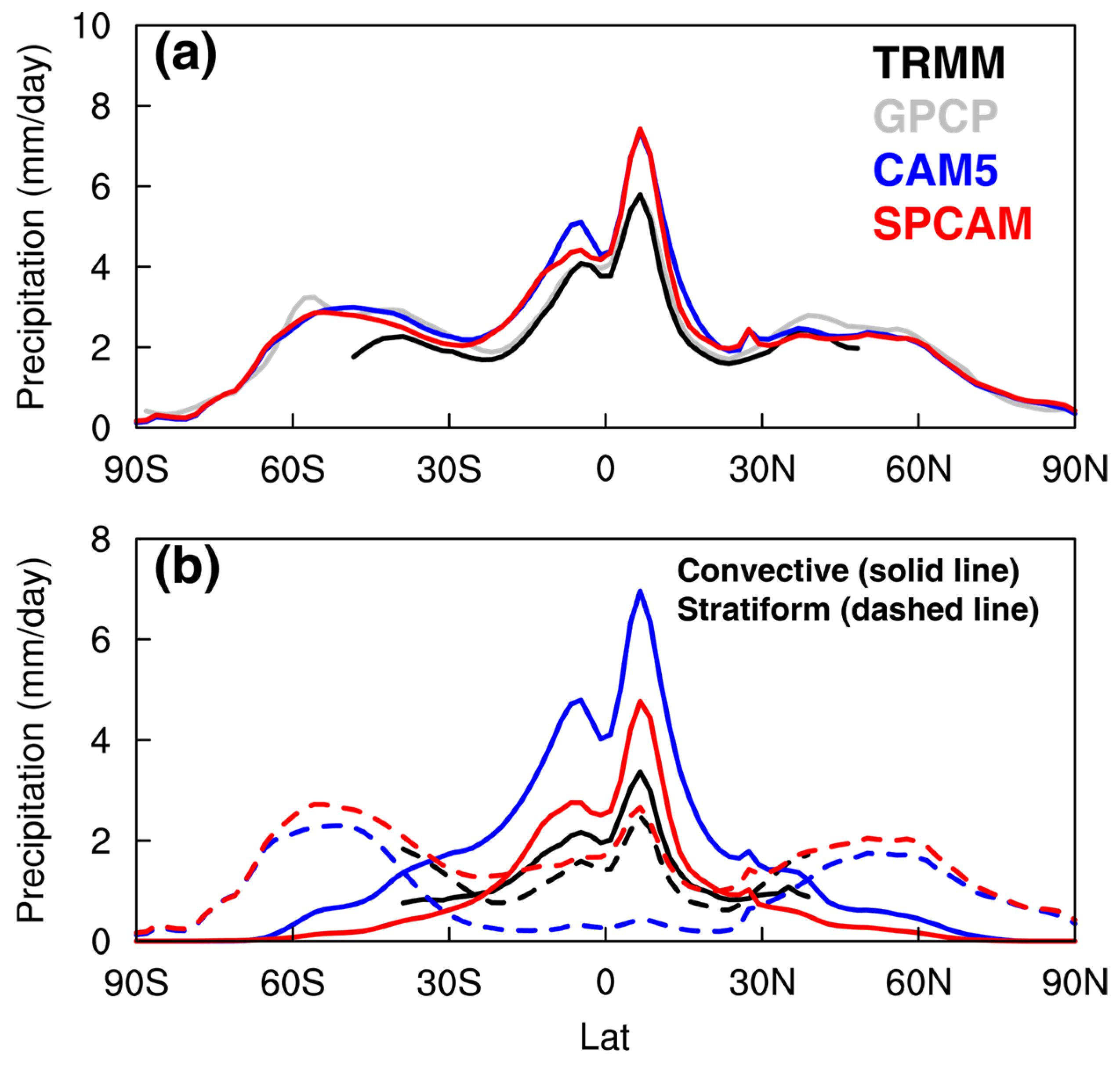
Figure 1 shows the zonal mean distribution of total, convective, and large-scale precipitation from GPCP and TRMM observations, as well as from CAM5 and SPCAM simulations. The overall total precipitation patterns are similar between CAM5 and SPCAM (Figure 1a and Figure S1). However, in the Southern Hemisphere tropics, CAM5 produces higher total precipitation than SPCAM, mainly due to a wetter Intertropical Convergence Zone (ITCZ) (Figure S1). Both models overestimate total precipitation in tropical and subtropical regions compared to observations, and agree well with observations at mid- and high-latitudes (Figure 1a). Poleward of 50°, CAM5 generates more rainfall via stratiform processes, with minimal difference in precipitation characteristics between the two models. Figure 1a and Figure S1 suggest that the total precipitation simulation is relatively insensitive to whether super-parameterization is adopted or not.

In contrast, CAM5 and SPCAM differ markedly in convective and large-scale precipitation components. In tropical convection regions, both observations and models indicate convective precipitation dominates over large-scale precipitation (Figure 1b). However, CAM5 shows a systematic bias. It severely overestimates convective precipitation and underestimates large-scale precipitation, while SPCAM agrees better with TRMM. The tropical–subtropical overestimation of total precipitation (Figure 1a) stems from different causes in each model. In SPCAM, it results from a slight overestimate of convective precipitation, whereas large-scale precipitation matches observations well. In CAM5, over 90% of tropical–subtropical rainfall comes from convective parameterization, far exceeding observations, while the simulated large-scale precipitation is significantly underestimated. The similar total precipitation but differing convective–stratiform distribution implies that CAM5’s parameterizations strongly affect precipitation type. Convective precipitation is overly active in CAM5. Such overestimation is common in conventional models [11], relating to both convective and microphysics schemes. For instance, under the same deep convection scheme, CAM5 produces more convective rain than CAM4 due to microphysical differences [33]. Interactions between convection and stratiform clouds also influence precipitation partitioning [39,40], with large-scale precipitation linked to low-level convergence and surface fluxes, while convective precipitation is affected by large-scale processes such as moisture divergence [41].

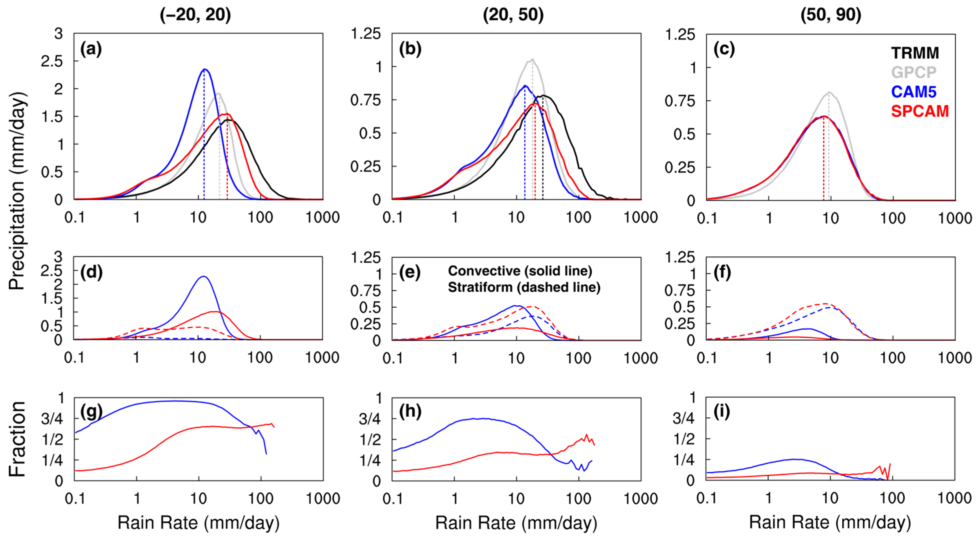
Bias lying in the partitioning between convective and large-scale precipitation greatly affects the simulation of precipitation intensity distribution. Figure 2 shows the distribution of total, convective, and large-scale precipitation, along with the convective precipitation ratio across intensity ranges and latitudes, in GPCP/TRMM observations and CAM5/SPCAM experiments. It is evident that while conventional GCMs capture the broad spatial pattern of mean precipitation, they show significant biases in frequency and intensity. In the tropics, CAM5 overrepresents weak precipitation and underrepresents strong events, with a mode around 12 mm day⁻¹. SPCAM, however, produces more heavy (>20 mm day⁻¹) precipitation and less light rain, yielding a mode near 40 mm day⁻¹, closer to observations (Figure 2a). The distributions in subtropical and mid-latitude regions are like those in tropical regions (Figure 2b,c). The weak mode in CAM5 is mainly convective in origin and stems from overestimated light and underestimated heavy precipitation, whereas both convective and large-scale components contribute in SPCAM (Figure 2d). The shift toward higher intensities in SPCAM reflects increased convective precipitation at higher intensities and reduced contribution at lower intensities, alongside a general rise in large-scale precipitation across all intensities compared to CAM5. The convective precipitation ratio is consistently higher in CAM5 than SPCAM within a relatively weak range of precipitation intensity across all latitudes (Figure 2g–i), indicating persistent overestimation of convective rain in conventional models [11].

3.2. Impacts on Aerosol Wet Deposition Fluxes

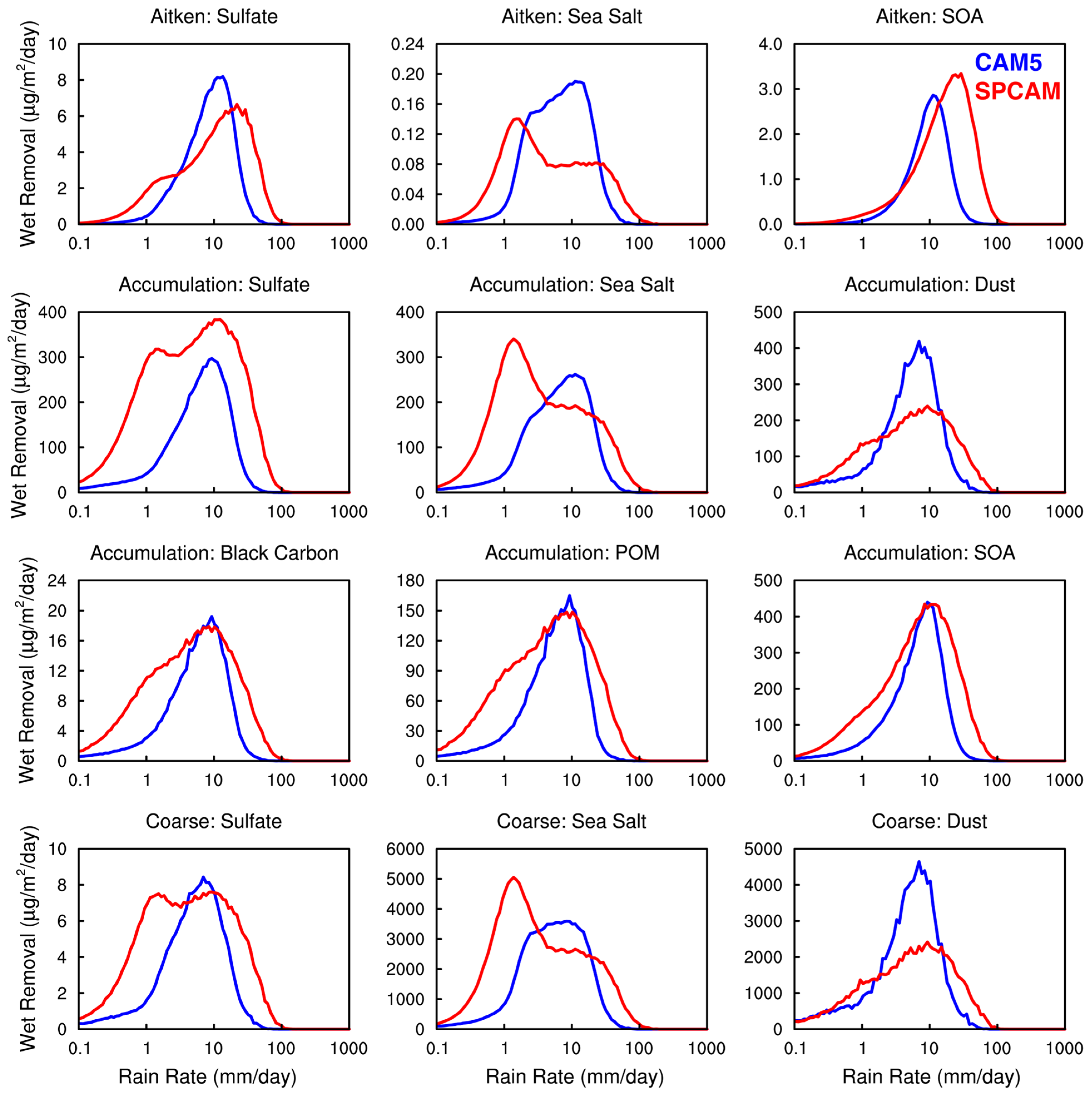
The misrepresentation of precipitation partitioning and frequency in CAM5 leads to corresponding systematic errors in simulated aerosol wet deposition. Figure 3 shows the distribution of wet deposition for aerosols of different types and sizes as a function of precipitation intensity in the tropics, as simulated by CAM5 and SPCAM. It should be noted that due to different treatment methods for aerosol activation, the absolute value of the total amount of aerosol wet deposition between the two simulations cannot be quantitatively compared. In CAM5, the wet deposition distribution for all aerosol types and sizes generally follows the pattern of precipitation distribution. However, the scavenging amount mode does not align with the precipitation amount mode, especially for coarse and accumulation mode particles (Figure 2a and Figure 3). Specifically, in CAM5, for sulfate, sea salt, and secondary organic aerosol (SOA) in the Aitken mode, the scavenging amount mode is approximately 8–10 mm day⁻¹, which is smaller than the precipitation amount mode of 12 mm day⁻¹. As the aerosol size increases to the coarse mode, the scavenging amount mode decreases to 7–8 mm day⁻¹ compared to the smaller-sized sulfate, sea salt, and dust. This reduction can be attributed to the higher scavenging coefficients of coarse-mode aerosols in below-cloud scavenging and the larger convective cloud activation fraction prescribed for coarse-mode sea salt and sulfate based on their hygroscopic properties. The characteristic that the scavenging amount mode is lower than the total precipitation mode further suggests that the frequency of light rain plays a more important role in regulating aerosol wet scavenging than the frequency of total precipitation. To confirm this, the spatial distributions of differences in light and total precipitation frequency between CAM5 and SPCAM are shown in Figure S2. Compared to total precipitation frequency, the decrease in light rain frequency is more significant, as the change in total precipitation frequency is the combined effect of a decrease in light rain frequency and an increase in heavy rain frequency. Due to the high hydrophilicity, sea salt is more sensitive to light rain and shows a steeper increase in wet deposition rate across all size modes as precipitation exceeds 1 mm day⁻¹. In SPCAM, the removal is efficiently driven by a broad range of rain rates, and the scavenging mode shifts toward higher precipitation rates consistent with a stronger precipitation mode except for sea salt. The shift in the wet removal mode to higher rain rates in SPCAM aligns with its more realistic, higher-mode precipitation distribution, demonstrating a greater physical consistency between its precipitation and removal processes. Sea salt exhibits a bimodal wet deposition distribution, with drizzle (0.1–1 mm day⁻¹) playing a significant role. The difference in the “scavenging mode” between CAM5 and SPCAM demonstrates that the model’s wet deposition is not just a passive consequence of its precipitation but is intrinsically tied to the (flawed) physical parameterizations that generate the rain.

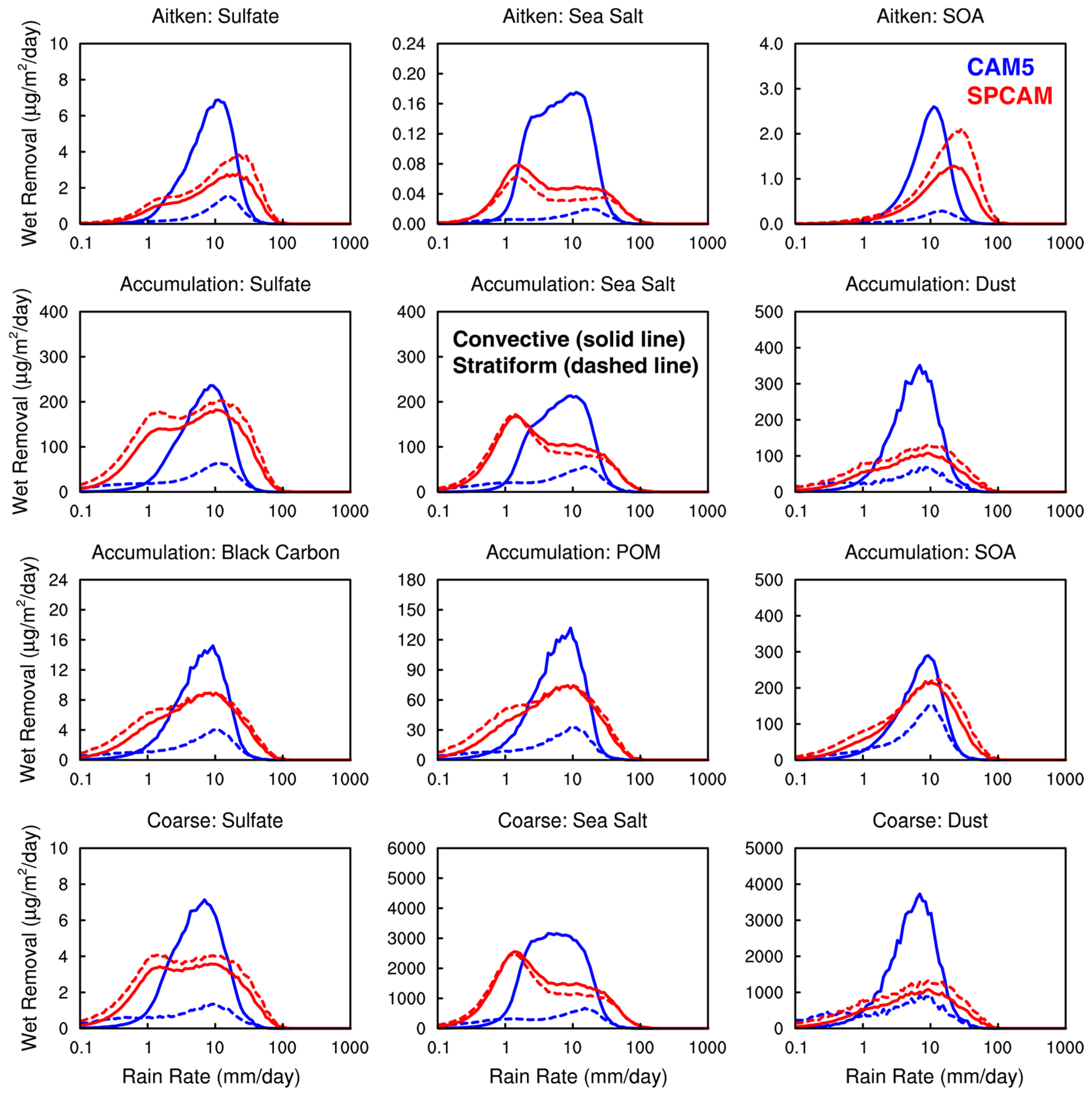
The differences in wet deposition between CAM5 and SPCAM can be explained by their simulated convective and stratiform deposition components (Figure 4). In CAM5, convective wet deposition dominates in the tropics, whereas SPCAM shows comparable convective and stratiform contributions, with slightly higher stratiform cloud deposition for most aerosol species and sizes. Biases in convective precipitation frequency in CAM5 (Figure S3) affect aerosol wet deposition across nearly all sizes and types. CAM5 overestimates convective precipitation frequency in the 1–20 mm day⁻¹ range and underestimates it outside this range (Figure S3a). Accordingly, CAM5 simulates higher convective wet deposition in the 2–20 mm day⁻¹ range but lower deposition at 0.1–2 mm day⁻¹ and above 20 mm day⁻¹ compared to SPCAM. CAM5 also significantly underestimates stratiform precipitation across all intensities, leading to consistently lower stratiform wet deposition for all aerosol types and sizes compared to SPCAM (Figure 4). In addition, the results of SPCAM show that the precipitation of stratiform clouds is less than that of convective clouds (Figure 2d), but the wet deposition of stratiform clouds is greater than that of convective clouds across most aerosol species and sizes (Figure 4). This indicates that the efficiency of stratiform cloud wet deposition is higher than that of convective wet deposition in SPCAM. This is mainly due to the high efficiency of stratiform in-cloud scavenging in removing activated aerosols in SPCAM, which indicates a significant deviation of CAM5 in this regard. We further calculated a simple mass scavenging efficiency index, fractional wet deposition efficiency, which is defined by the fraction of wet deposition flux (%) per unit precipitation (mm day⁻¹), separately for convective and stratiform rain. The results (Table S2) show that in both CAM5 and SPCAM, stratiform rain has a higher scavenging efficiency than convective rain. In CAM5, the scavenging efficiency of convective rain is notably lower, consistent with its lack of explicit representation of convective-cloud-borne aerosols and the corresponding scavenging.

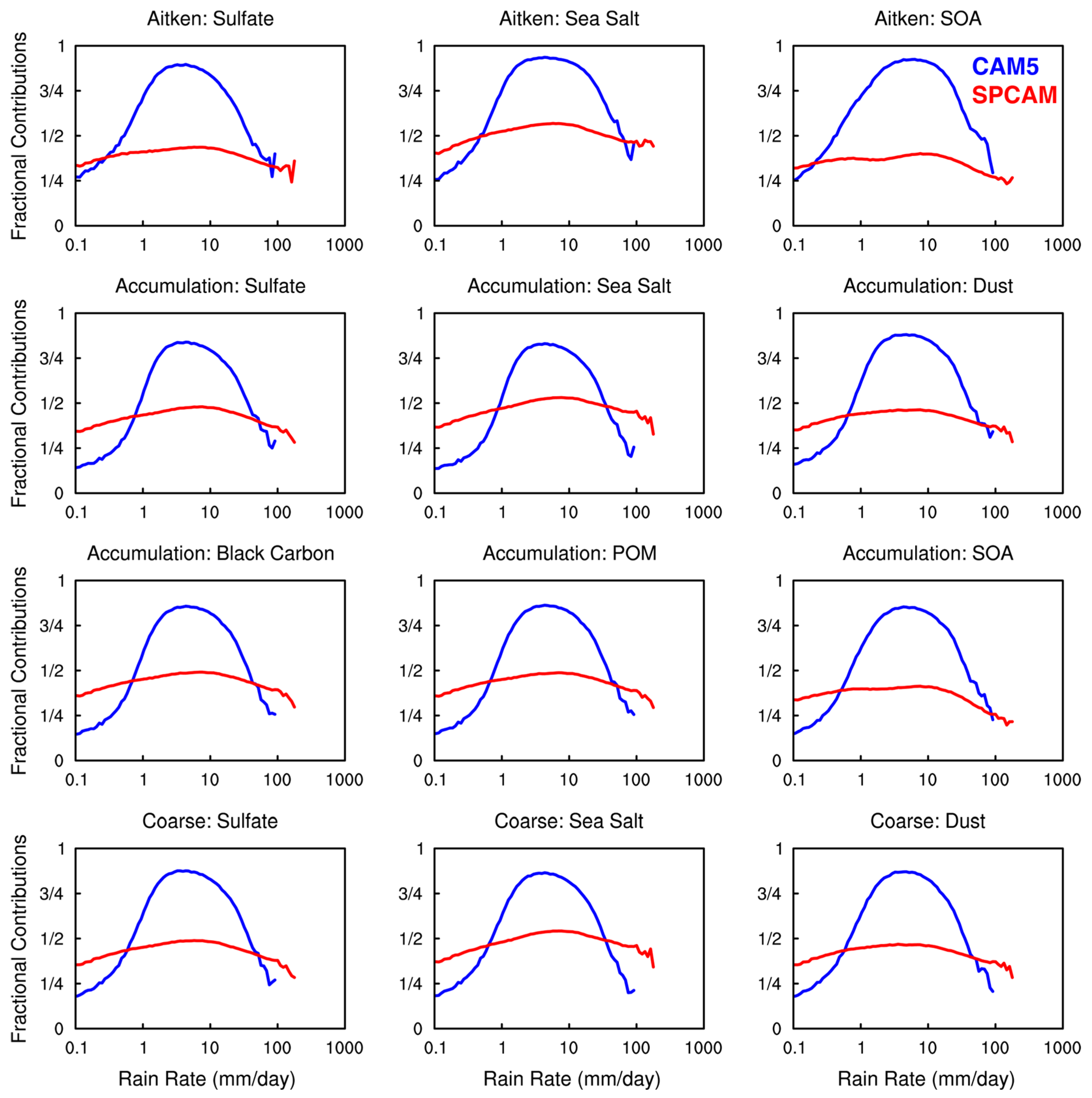
The fractional contribution of convective wet deposition to total wet deposition in the tropics (Figure 5) highlights systematic errors in CAM5. In SPCAM, even in the tropics, convective deposition accounts for less than 50% of total wet deposition for most aerosols across all precipitation rates. Sea salt is an exception, slightly exceeding 50% at around 10 mm day⁻¹. For all aerosols, convective deposition accounts for 47.6% of total wet deposition, with a contribution of 68.3% from convective light rain (1–20 mm day⁻¹), while large-scale deposition accounts for 52.4% of total wet deposition, with a contribution of 62.9% from large-scale light rain, leading to a total contribution of 65.5% from light rain removal. In contrast, CAM5 overestimates both convective and light rain contributions, with convective wet deposition accounting for over half of total deposition in the 1–20 mm day⁻¹ range. For Aitken-mode sulfate, sea salt, and SOA, deposition is almost entirely convective near 10 mm day⁻¹. For all aerosols in CAM5, convective deposition accounts for 74.2% of total wet deposition, with a contribution of 92.2% from convective light rain, while large-scale deposition accounts for 25.8% of total wet deposition, with a contribution of 60.4% from large-scale light rain, leading to a total contribution of 84.0% from light rain removal. Furthermore, in CAM5, convective precipitation accounts for over half of total precipitation at 0.1–1 mm day⁻¹ (Figure 2g), yet convective wet deposition in that range is less than half of the total, indicating lower wet scavenging efficiency per unit convective precipitation compared to stratiform rain. This discrepancy is partly because in CAM5, convective precipitation does not remove cloud-borne aerosols, which is an inherent limitation of the convective scheme. In SPCAM, for precipitation rates between 0.2 and 8 mm day⁻¹, convective precipitation is less frequent than stratiform (Figure S3d), especially in the 0.2–1 mm day⁻¹ range, where it constitutes about 1/8 of total rain (Figure 2g), yet contributes over 1/4 of convective wet deposition (Figure 5). At rates above 10 mm day⁻¹, convective rain contributes over half of total precipitation (Figure 2g) but less than half of wet deposition (Figure 5). This suggests that in SPCAM, light convective rain has higher scavenging efficiency than light stratiform rain, whereas heavy convective rain is less efficient than heavy stratiform rain.

Overall, the curve distribution in subtropical, mid-latitude, and high-latitude regions is like that in tropical regions, and the conclusions obtained are consistent (Figures S4–S9). These differences imply that CAM5 not only misallocates wet deposition between convective and stratiform components due to biased precipitation partitioning but also may misrepresent the scavenging efficiencies of convective and stratiform rain due to empirical parameterizations, leading to potential deviations of simulated wet deposition from real-world behavior.

3.3. Consequences for Simulated Aerosol Burdens

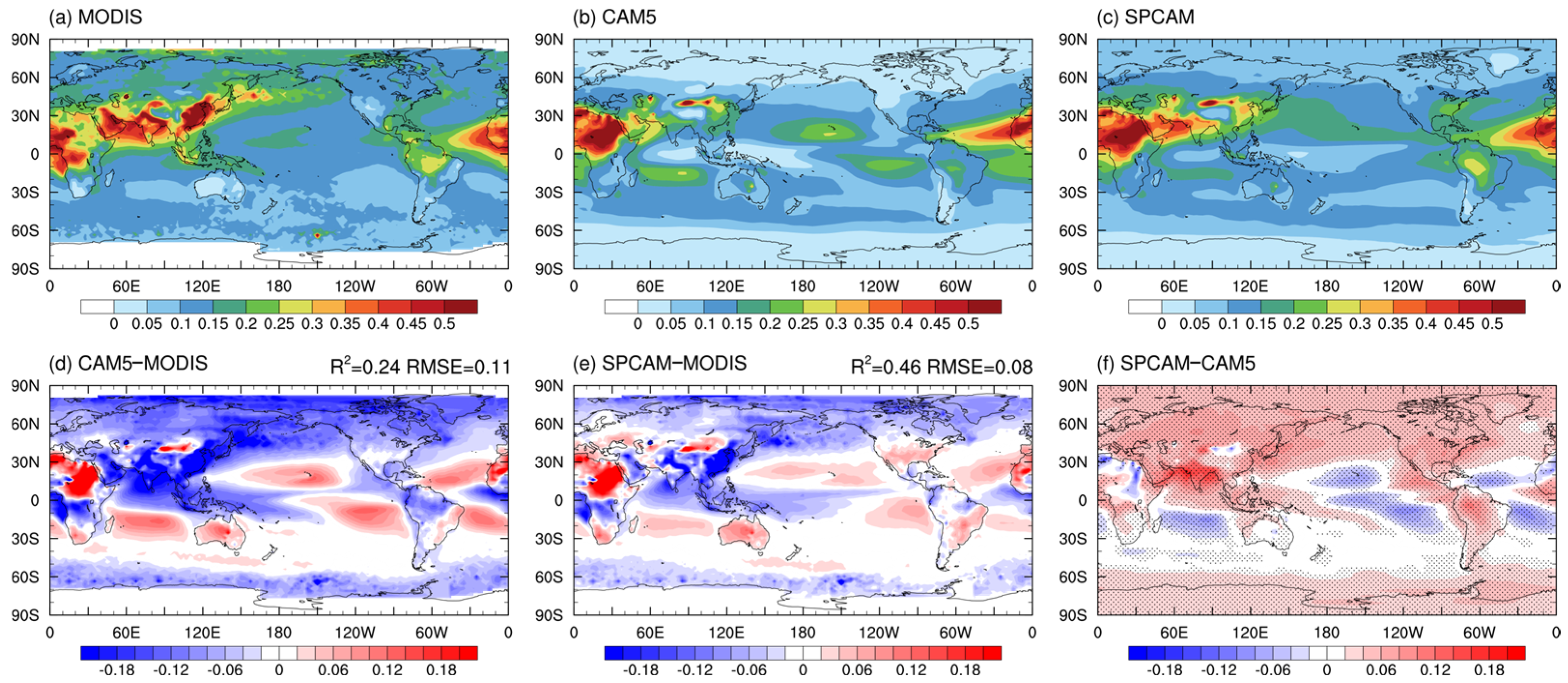
The cumulative effect of biased wet deposition fluxes is a significant error in the simulated atmospheric aerosol burdens. Figure 6 presents the annual mean aerosol optical depth (AOD) from MODIS Aqua observation alongside CAM5 and SPCAM simulations. While both models capture the major aerosol source regions, CAM5 exhibits a consistent negative bias in AOD over continental regions in the Northern Hemisphere (e.g., East Asia, Eastern North America) compared to MODIS. This is paired with a positive bias over remote oceanic regions. The difference field (SPCAM minus CAM5) in Figure 6f shows an alleviation of the bias. CAM5 simulates lower aerosol burdens downwind of major anthropogenic source regions and higher burdens over the oceans compared to SPCAM. Besides the inherent missing of aerosol emission sources [42], this spatial pattern is also a direct consequence of the wet deposition biases (Figure S10). The excessive and premature removal of aerosols by frequent light convective rain in CAM5 efficiently scavenges pollutants near their source regions, preventing their long-range transport. This leads to an underestimation of continental AOD and an overestimation of marine AOD, as fewer aerosols survive to be transported to remote areas. Globally, CAM5 underestimates the lifetimes of all species of aerosols compared to SPCAM (

Table 1. Global averages of the mean atmospheric lifetime (days) for sulfate, sea salt, dust, black carbon (BC), primary organic matter (POM), and secondary organic aerosol (SOA) in CAM5 and SPCAM runs.

Lifetime (Days)	Sulfate	Sea Salt	Dust	BC	POM	SOA
CAM5	3.40	0.72	2.51	3.73	4.04	3.55
SPCAM	4.38	0.75	3.11	4.59	4.87	3.95

and Figure S11). The more physical representation of precipitation in SPCAM allows for a more realistic transport and removal pathway, resulting in a better agreement with the observed spatial distribution of AOD.

4. Conclusions and Discussions

This study demonstrates that conventional parameterized GCM like CAM5 exhibits systematic biases in precipitation partitioning, including overproduction of light convective rain, underestimation of heavy convective precipitation, and an excessively high convective-to-total precipitation ratio. These biases propagate directly into significant errors in the simulated aerosol life cycle. The excessive reliance on convective parameterization in CAM5 creates a distorted reality where aerosols are scavenged too efficiently and too close to their sources, leading to an unrealistic representation of their atmospheric distribution and lifetime when benchmarked against SPCAM. The core issue lies in the physical disconnect within the model framework. In CAM5, convective precipitation is a diagnostic output of a parameterization scheme designed to stabilize the large-scale atmosphere, not a physically consistent representation of cloud processes. This leads to the well-known “drizzling” bias [11,43], which our study explicitly links to aerosol wet deposition [6,7].

We acknowledge that the precipitation rate bins used (Figure 2, Figure 3, Figure 4 and Figure 5) integrate the effects of event frequency, intensity, and, for parameterized convection, sub-grid area. Fully disentangling the individual contributions of these factors would require targeted sensitivity experiments [5] or advanced diagnostic techniques, which is a valuable direction for future work. However, the consistent pattern of excessive occurrence of light rain in CAM5 (Figure S3), coupled with the established understanding that long-term scavenging is strongly governed by precipitation frequency [6,7], provides robust support for our interpretation that the bias in frequency distribution is the principal driver of the wet deposition errors. Furthermore, our results are consistent with Hou et al. [5], in which the idealized sensitivity experiments demonstrated that precipitation frequency, rather than intensity, is the dominant control on long-term aerosol wet removal.

The implication extends beyond a mere technical model bias. By underestimating aerosol burdens over continents and overestimating them over remote oceans (Figure 6), CAM5 likely miscalculates the magnitude and spatial pattern of the radiative forcing. For example, an underestimation of anthropogenic aerosol loading over industrial regions could lead to an underestimation of the global dimming effect and a consequent overestimation of the warming attributable to greenhouse gases alone [44]. This has direct consequences for the interpretation of historical climate change and the reliability of future projections from models employing similar convective parameterizations. Furthermore, our findings have important ramifications for air quality studies. The premature removal of aerosols near source regions in CAM5 and similar models would lead to an underestimation of long-range transport of air pollution, such as the cross-Pacific transport of Asian aerosols. This could affect policy decisions based on model simulations of regional air quality and its transboundary impacts.

While SPCAM provides a powerful tool for process-level evaluation, its computational cost prohibits its use for long-term, ensemble climate simulations. Therefore, the solution is not to replace all GCMs with SPCAM but to use its insights to inform the development of next-generation parameterizations. The development of “scale-aware” convective schemes designed for higher-resolution models is a step in the right direction [45]. Our results suggest that to achieve reliable projections of both air quality and climate change, future scheme development must prioritize the accurate representation of the precipitation partitioning and intensity distribution, not just the total rainfall amount. Benchmarking CAM5 against SPCAM, as done in this study, provides an essential pathway for this improvement.

References

1. Szopa, S.; Naik, V.; Adhikary, B.; Artaxo, P.; Berntsen, T.; Collins, W.D.; Fuzzi, S.; Gallardo, L.; Kiendler-Scharr, A.; Klimont, Z.; et al. Short-Lived Climate Forcers. In Climate Change 2021: The Physical Science Basis. Contribution of Working Group I to the Sixth Assessment Report of the Intergovernmental Panel on Climate Change; Masson-Delmotte, V., Zhai, P., Pirani, A., Connors, S.L., Péan, C., Berger, S., Caud, N., Chen, Y., Goldfarb, L., Gomis, M.I., et al., Eds.; Cambridge University Press: Cambridge, UK; New York, NY, USA, 2021; pp. 817–922. [Google Scholar]
2. Twomey, S. The Influence of Pollution on the Shortwave Albedo of Clouds. J. Atmos. Sci. 1977, 34, 1149–1152. [Google Scholar] [CrossRef]
3. Burnett, R.; Chen, H.; Szyszkowicz, M.; Fann, N.; Hubbell, B.; Pope, C.A.; Apte, J.S.; Brauer, M.; Cohen, A.; Weichenthal, S.; et al. Global Estimates of Mortality Associated with Long-Term Exposure to Outdoor Fine Particulate Matter. Proc. Natl. Acad. Sci. USA 2018, 115, 201803222. [Google Scholar] [CrossRef]
4. Ohata, S.; Moteki, N.; Mori, T.; Koike, M.; Kondo, Y. A Key Process Controlling the Wet Removal of Aerosols: New Observational Evidence. Sci. Rep. 2016, 6, 34113. [Google Scholar] [CrossRef]
5. Hou, P.; Wu, S.; McCarty, J.L.; Gao, Y. Sensitivity of Atmospheric Aerosol Scavenging to Precipitation Intensity and Frequency in the Context of Global Climate Change. Atmos. Chem. Phys. 2018, 18, 8173–8182. [Google Scholar] [CrossRef]
6. Wang, Y.; Xia, W.; Liu, X.; Xie, S.; Lin, W.; Tang, Q.; Ma, H.-Y.; Jiang, Y.; Wang, B.; Zhang, G.J. Disproportionate Control on Aerosol Burden by Light Rain. Nat. Geosci. 2021, 14, 72–76. [Google Scholar] [CrossRef]
7. Xia, W.; Wang, Y.; Zhang, G.J.; Wang, B. Light Precipitation Rather than Total Precipitation Determines Aerosol Wet Removal. Environ. Sci. Technol. 2024, 58, 19222–19230. [Google Scholar] [CrossRef] [PubMed]
8. Griffiths, P.T.; Wilcox, L.J.; Allen, R.J.; Naik, V.; O’Connor, F.M.; Prather, M.; Archibald, A.; Brown, F.; Deushi, M.; Collins, W.; et al. Opinion: The Role of AerChemMIP in Advancing Climate and Air Quality Research. Atmos. Chem. Phys. 2025, 25, 8289–8328. [Google Scholar] [CrossRef]
9. Arakawa, A.; Schubert, W.H. Interaction of a Cumulus Cloud Ensemble with the Large-Scale Environment, Part I. J. Atmos. Sci. 1974, 31, 674–701. [Google Scholar] [CrossRef]
10. Xia, W.; Wang, Y.; Zhang, G.J.; Cui, Z.; Wang, B.; He, Y.; Wang, X. Unexpected Changes of Aerosol Burdens with Decreased Convection in the Context of Scale-Aware Convection Schemes. Geophys. Res. Lett. 2022, 49, e2022GL099008. [Google Scholar] [CrossRef]
11. Chen, D.; Dai, A.; Hall, A. The Convective-To-Total Precipitation Ratio and the “Drizzling” Bias in Climate Models. J. Geophys. Res. Atmos. 2021, 126, e2020JD034198. [Google Scholar] [CrossRef]
12. Wang, Y.; Xia, W.; Zhang, G.J. What Rainfall Rates Are Most Important to Wet Removal of Different Aerosol Types? Atmos. Chem. Phys. 2021, 21, 16797–16816. [Google Scholar] [CrossRef]
13. Wang, Y.; Zhang, G.J.; Craig, G.C. Stochastic Convective Parameterization Improving the Simulation of Tropical Precipitation Variability in the NCAR CAM5. Geophys. Res. Lett. 2016, 43, 6612–6619. [Google Scholar] [CrossRef]
14. Na, Y.; Fu, Q.; Kodama, C. Precipitation Probability and Its Future Changes from a Global Cloud-Resolving Model and CMIP6 Simulations. J. Geophys. Res. Atmos. 2020, 125, e2019JD031926. [Google Scholar] [CrossRef]
15. Liu, X.; Easter, R.C.; Ghan, S.J.; Zaveri, R.; Rasch, P.; Shi, X.; Lamarque, J.-F.; Gettelman, A.; Morrison, H.; Vitt, F.; et al. Toward a Minimal Representation of Aerosols in Climate Models: Description and Evaluation in the Community Atmosphere Model CAM5. Geosci. Model. Dev. 2012, 5, 709–739. [Google Scholar] [CrossRef]
16. Khairoutdinov, M.; Randall, D.; DeMott, C. Simulations of the Atmospheric General Circulation Using a Cloud-Resolving Model as a Superparameterization of Physical Processes. J. Atmos. Sci. 2005, 62, 2136–2154. [Google Scholar] [CrossRef]
17. Wang, M.; Ghan, S.; Easter, R.; Ovchinnikov, M.; Liu, X.; Kassianov, E.; Qian, Y.; Gustafson, W.I., Jr.; Larson, V.E.; Schanen, D.P.; et al. The Multi-Scale Aerosol-Climate Model PNNL-MMF: Model Description and Evaluation. Geosci. Model. Dev. 2011, 4, 137–168. [Google Scholar] [CrossRef]
18. Kooperman, G.J.; Pritchard, M.S.; Burt, M.A.; Branson, M.D.; Randall, D.A. Impacts of Cloud Superparameterization on Projected Daily Rainfall Intensity Climate Changes in Multiple Versions of the Community Earth System Model. J. Adv. Model. Earth Syst. 2016, 8, 1727–1750. [Google Scholar] [CrossRef]
19. Neale, R.B.; Chen, C.-C.; Gettelman, A.; Lauritzen, P.H.; Park, S.; Williamson, D.L.; Conley, A.J.; Garcia, R.; Kinnison, D.; Lamarque, J.-F. Description of the NCAR Community Atmosphere Model (CAM 5.0). NCAR Tech. Note Ncar/Tn-486+ STR 2010, 1, 1–12. [Google Scholar]
20. Zhang, G.J.; McFarlane, N.A. Sensitivity of Climate Simulations to the Parameterization of Cumulus Convection in the Canadian Climate Centre General Circulation Model. Atmos. Ocean. 1995, 33, 407–446. [Google Scholar] [CrossRef]
21. Neale, R.B.; Richter, J.H.; Jochum, M. The Impact of Convection on ENSO: From a Delayed Oscillator to a Series of Events. J. Clim. 2008, 21, 5904–5924. [Google Scholar] [CrossRef]
22. Park, S.; Bretherton, C.S. The University of Washington Shallow Convection and Moist Turbulence Schemes and Their Impact on Climate Simulations with the Community Atmosphere Model. J. Clim. 2009, 22, 3449–3469. [Google Scholar] [CrossRef]
23. Morrison, H.; Gettelman, A. A New Two-Moment Bulk Stratiform Cloud Microphysics Scheme in the Community Atmosphere Model, Version 3 (CAM3). Part I: Description and Numerical Tests. J. Clim. 2008, 21, 3642–3659. [Google Scholar] [CrossRef]
24. Morrison, H.; Curry, J.A.; Khvorostyanov, V.I. A New Double-Moment Microphysics Parameterization for Application in Cloud and Climate Models. Part I: Description. J. Atmos. Sci. 2005, 62, 1665–1677. [Google Scholar] [CrossRef]
25. Lamarque, J.-F.; Bond, T.C.; Eyring, V.; Granier, C.; Heil, A.; Klimont, Z.; Lee, D.; Liousse, C.; Mieville, A.; Owen, B.; et al. Historical (1850–2000) Gridded Anthropogenic and Biomass Burning Emissions of Reactive Gases and Aerosols: Methodology and Application. Atmos. Chem. Phys. 2010, 10, 7017–7039. [Google Scholar] [CrossRef]
26. Zhang, Z.; Wang, Y.; Zhang, G.J.; Xing, C.; Xia, W.; Yang, M. Light Rain Exacerbates Extreme Humid Heat. Nat. Commun. 2024, 15, 7326. [Google Scholar] [CrossRef]
27. Suhas, E.; Zhang, G.J. Evaluating Convective Parameterization Closures Using Cloud-resolving Model Simulation of Tropical Deep Convection. J. Geophys. Res. Atmos. 2015, 120, 1260–1277. [Google Scholar] [CrossRef]
28. Huffman, G.J.; Bolvin, D.T. TRMM and Other Data Precipitation Data Set Documentation. NASA Greenbelt USA 2013, 28, 1. [Google Scholar]
29. Adler, R.F.; Huffman, G.J.; Chang, A.; Ferraro, R.; Xie, P.-P.; Janowiak, J.; Rudolf, B.; Schneider, U.; Curtis, S.; Bolvin, D.; et al. The Version-2 Global Precipitation Climatology Project (GPCP) Monthly Precipitation Analysis (1979–Present). J. Hydrometeorol. 2003, 4, 1147–1167. [Google Scholar] [CrossRef]
30. Huffman, G.J.; Bolvin, D.T.; Nelkin, E.J.; Wolff, D.B.; Adler, R.F.; Gu, G.; Hong, Y.; Bowman, K.P.; Stocker, E.F. The TRMM Multisatellite Precipitation Analysis (TMPA): Quasi-Global, Multiyear, Combined-Sensor Precipitation Estimates at Fine Scales. J. Hydrometeorol. 2007, 8, 38–55. [Google Scholar] [CrossRef]
31. Kummerow, C.; Hong, Y.; Olson, W.S.; Yang, S.; Adler, R.F.; McCollum, J.; Ferraro, R.; Petty, G.; Shin, D.-B.; Wilheit, T.T. The Evolution of the Goddard Profiling Algorithm (GPROF) for Rainfall Estimation from Passive Microwave Sensors. J. Appl. Meteorol. 2001, 40, 1801–1820. [Google Scholar] [CrossRef]
32. Ehsan, M.A.; Almazroui, M.; Yousef, A. Impact of Different Cumulus Parameterization Schemes in SAUDI-KAU AGCM. Earth Syst. Environ. 2017, 1, 3. [Google Scholar] [CrossRef]
33. Chen, D.; Dai, A. Precipitation Characteristics in the Community Atmosphere Model and Their Dependence on Model Physics and Resolution. J. Adv. Model. Earth Syst. 2019, 11, 2352–2374. [Google Scholar] [CrossRef]
34. Alemohammad, S.H.; McColl, K.A.; Konings, A.G.; Entekhabi, D.; Stoffelen, A. Characterization of Precipitation Product Errors across the United States Using Multiplicative Triple Collocation. Hydrol. Earth Syst. Sci. 2015, 19, 3489–3503. [Google Scholar] [CrossRef]
35. Rossow, W.B.; Mekonnen, A.; Pearl, C.; Goncalves, W. Tropical Precipitation Extremes. J. Clim. 2013, 26, 1457–1466. [Google Scholar] [CrossRef][Green Version]
36. Wolff, D.B.; Fisher, B.L. Assessing the Relative Performance of Microwave-Based Satellite Rain-Rate Retrievals Using TRMM Ground Validation Data. J. Appl. Meteorol. Clim. 2009, 48, 1069–1099. [Google Scholar] [CrossRef]
37. Platnick, S.; Meyer, K.G.; King, M.D.; Wind, G.; Amarasinghe, N.; Marchant, B.; Arnold, G.T.; Zhang, Z.; Hubanks, P.A.; Holz, R.E.; et al. The MODIS Cloud Optical and Microphysical Products: Collection 6 Updates and Examples from Terra and Aqua. IEEE Trans. Geosci. Remote Sens. 2017, 55, 502–525. [Google Scholar] [CrossRef] [PubMed]
38. Kooperman, G.J.; Pritchard, M.S.; O’Brien, T.A.; Timmermans, B.W. Rainfall from Resolved Rather Than Parameterized Processes Better Represents the Present-Day and Climate Change Response of Moderate Rates in the Community Atmosphere Model. J. Adv. Model. Earth Syst. 2018, 10, 971–988. [Google Scholar] [CrossRef]
39. Held, I.M.; Zhao, M.; Wyman, B. Dynamic Radiative–Convective Equilibria Using GCM Column Physics. J. Atmos. Sci. 2007, 64, 228–238. [Google Scholar] [CrossRef]
40. Lin, Y.; Zhao, M.; Ming, Y.; Golaz, J.-C.; Donner, L.J.; Klein, S.A.; Ramaswamy, V.; Xie, S. Precipitation Partitioning, Tropical Clouds, and Intraseasonal Variability in GFDL AM2. J. Clim. 2013, 26, 130206114111004. [Google Scholar] [CrossRef]
41. Sakaguchi, K.; Leung, L.R.; Burleyson, C.D.; Xiao, H.; Wan, H. Role of Troposphere-Convection-Land Coupling in the Southwestern Amazon Precipitation Bias of the Community Earth System Model Version 1 (CESM1). J. Geophys. Res. Atmos. 2018, 123, 8374–8399. [Google Scholar] [CrossRef]
42. Hoesly, R.M.; Smith, S.J.; Feng, L.; Klimont, Z.; Janssens-Maenhout, G.; Pitkanen, T.; Seibert, J.J.; Vu, L.; Andres, R.J.; Bolt, R.M.; et al. Historical (1750–2014) Anthropogenic Emissions of Reactive Gases and Aerosols from the Community Emissions Data System (CEDS). Geosci. Model. Dev. 2017, 11, 369–408. [Google Scholar] [CrossRef]
43. Dai, A. Precipitation Characteristics in Eighteen Coupled Climate Models. J. Clim. 2006, 19, 4605–4630. [Google Scholar] [CrossRef]
44. Wang, Y.; Xia, W.; Zhang, G.J.; Wang, B.; Lin, G. Impacts of Suppressing Excessive Light Rain on Aerosol Radiative Effects and Health Risks. J. Geophys. Res. Atmos. 2022, 127, e2021JD036204. [Google Scholar] [CrossRef]
45. Ahn, M.-S.; Kang, I.-S. A Practical Approach to Scale-Adaptive Deep Convection in a GCM by Controlling the Cumulus Base Mass Flux. npj Clim. Atmos. Sci. 2018, 1, 13. [Google Scholar] [CrossRef]
Figure 1. Zonal mean (a) total (solid line), (b) convective (solid line) and large-scale (dashed line) precipitation in CAM5 (blue), SPCAM (red), TRMM (black). Zonal mean total rain in GPCP (green) is also shown in (a). The total precipitation of TRMM in (a) comes from the TRMM 3B43 product, and the convective and large-scale precipitation of TRMM in (b) comes from the TRMM 3A12 product.
Remotesensing 18 00151 g001
Figure 2. Precipitation amount distributions of (ac) total (solid line), (df) convective (solid line) and stratiform (dashed line) contributions, and (gi) fractional contributions of convective to total precipitation over (a,d,g) (20°S–20°N), (b,e,h) (20°N–50°N), and (c,f,i) (50°N–90°N) for TRMM (black), GPCP (grey), CAM5 (blue), and SPCAM (red) runs. The vertical dashed lines in (ac) indicate the rain rate where the precipitation amount modes are located. The units for subplots (af) are mm day−1, while the amount distributions are scaled by ln R = R / R , which has a unit of mm day−1/mm day−1, and is thus a unitless scaling term. The x-axis (precipitation rate) indicates the daily precipitation intensity and is on a logarithmic scale.
Remotesensing 18 00151 g002
Figure 3. Amount distributions of aerosol wet removal over (20°S–20°N) in CAM5 (blue) and SPCAM (red) runs. The units for all subplots are µg m−2 day−1, while the amount distributions are scaled by ln R = R / R , which has a unit of mm day−1/mm day−1, and is thus a unitless scaling term. The x-axis (precipitation rate) indicates the daily precipitation intensity and is on a logarithmic scale.
Remotesensing 18 00151 g003
Figure 4. Amount distributions of aerosol wet removal by convective (solid line) and stratiform (dashed line) precipitation over (20°S–20°N) in CAM5 (blue) and SPCAM (red) runs. The units for all subplots are µg m−2 day−1, while the amount distributions are scaled by ln R = R / R , which has a unit of mm day−1/mm day−1, and is thus a unitless scaling term. The x-axis (precipitation rate) indicates the daily precipitation intensity and is on a logarithmic scale.
Remotesensing 18 00151 g004
Figure 5. Fractional contributions of wet removal of aerosols from convective clouds to the total amount of aerosol wet deposition over (20°S–20°N) in CAM5 (blue) and SPCAM (red) runs. The distributions are scaled by ln R = R / R , which has a unit of mm day−1/mm day−1, and is thus a unitless scaling term. The x-axis (precipitation rate) indicates the daily precipitation intensity and is on a logarithmic scale.
Remotesensing 18 00151 g005
Figure 6. Global distributions of AOD in MODIS, CAM5 and SPCAM and their differences. The stippled areas in (f) indicate that the difference between CAM5 and SPCAM is statistically significant at the 0.05 level. Values in the top right corner for the differences between model simulations and observations are the coefficient of determination (R2) and the weighted root-mean-square error (RMSE).
Remotesensing 18 00151 g006