
A Regional Ionospheric TEC Map Assimilation Method Considering Temporal Scale During Geomagnetic Storms


Abstract
1. Introduction
2. Materials and Methods
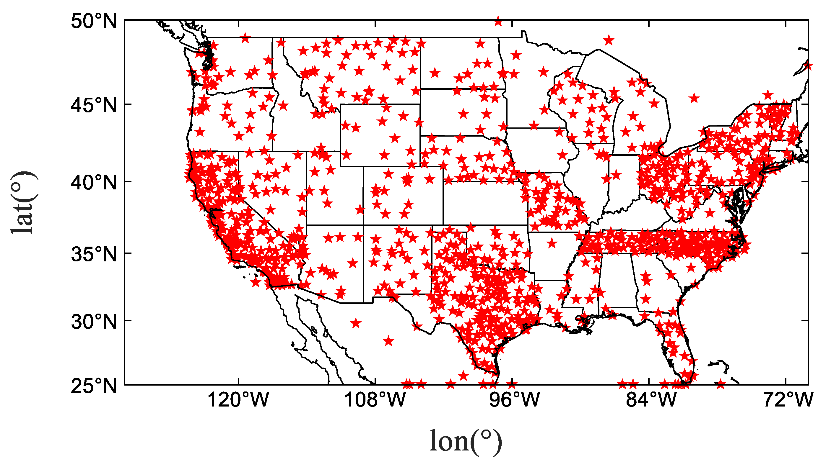
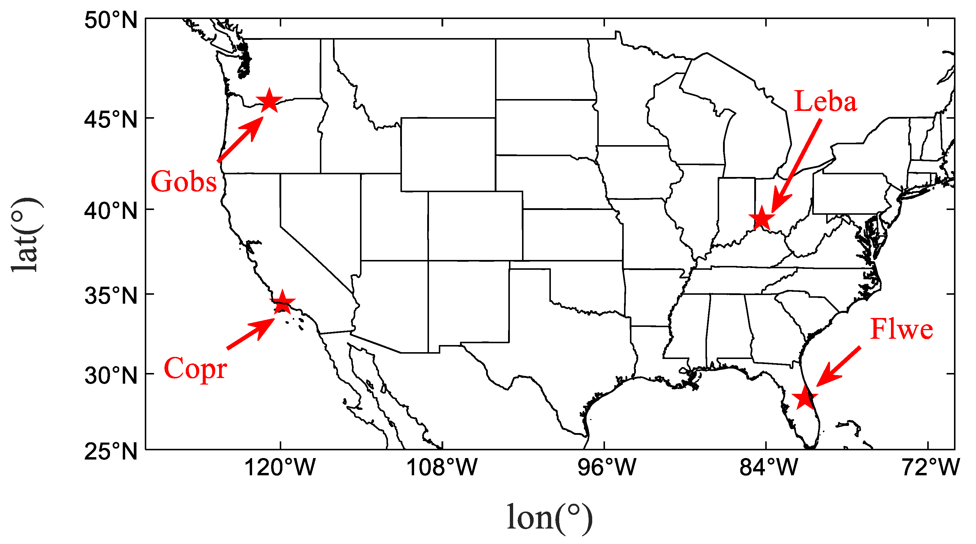
2.1. US CORS Station Data
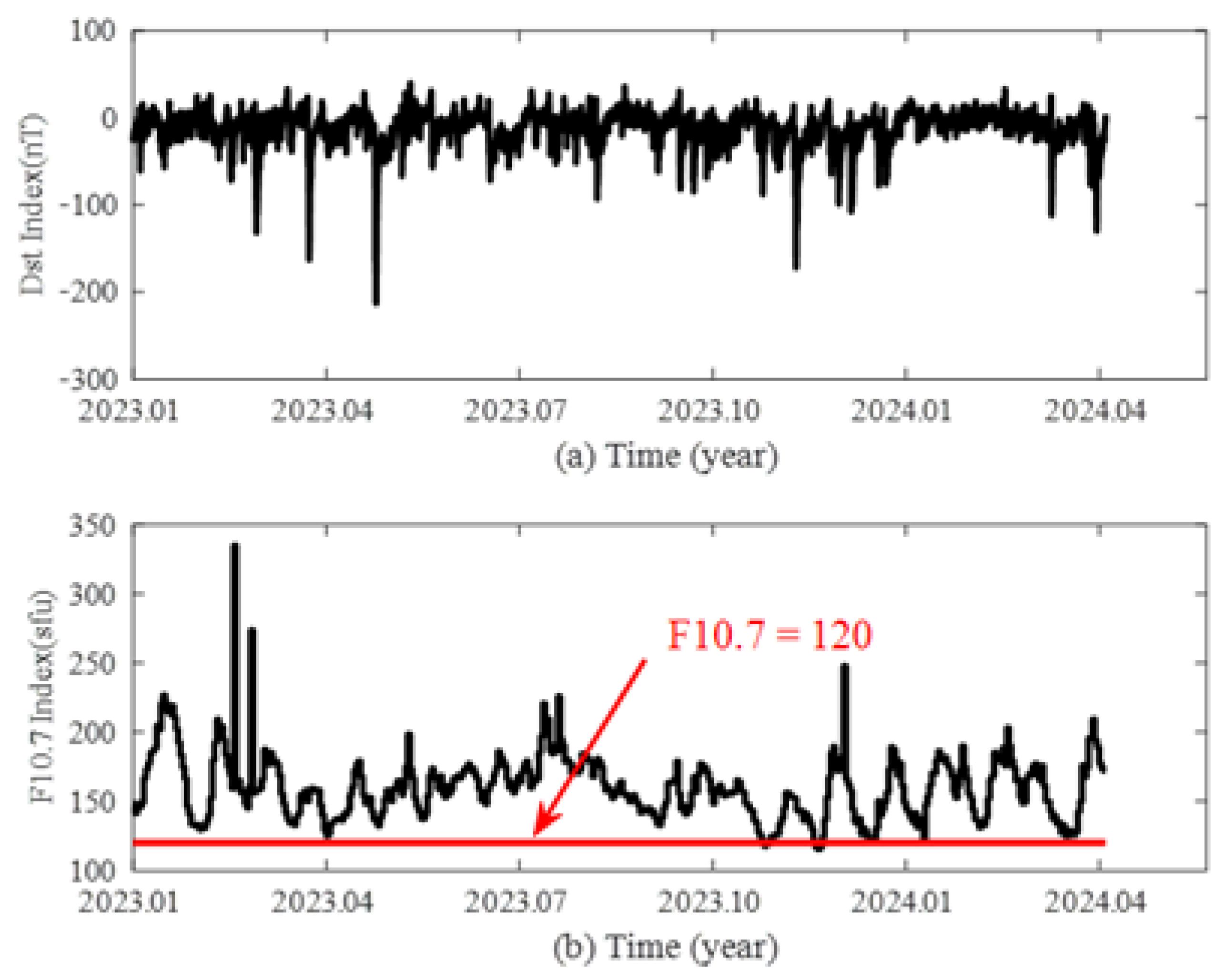
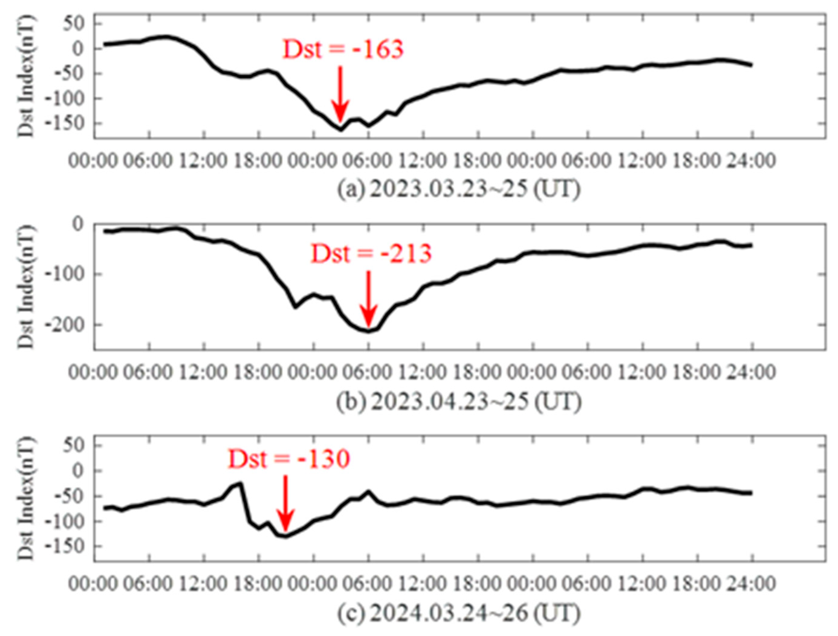
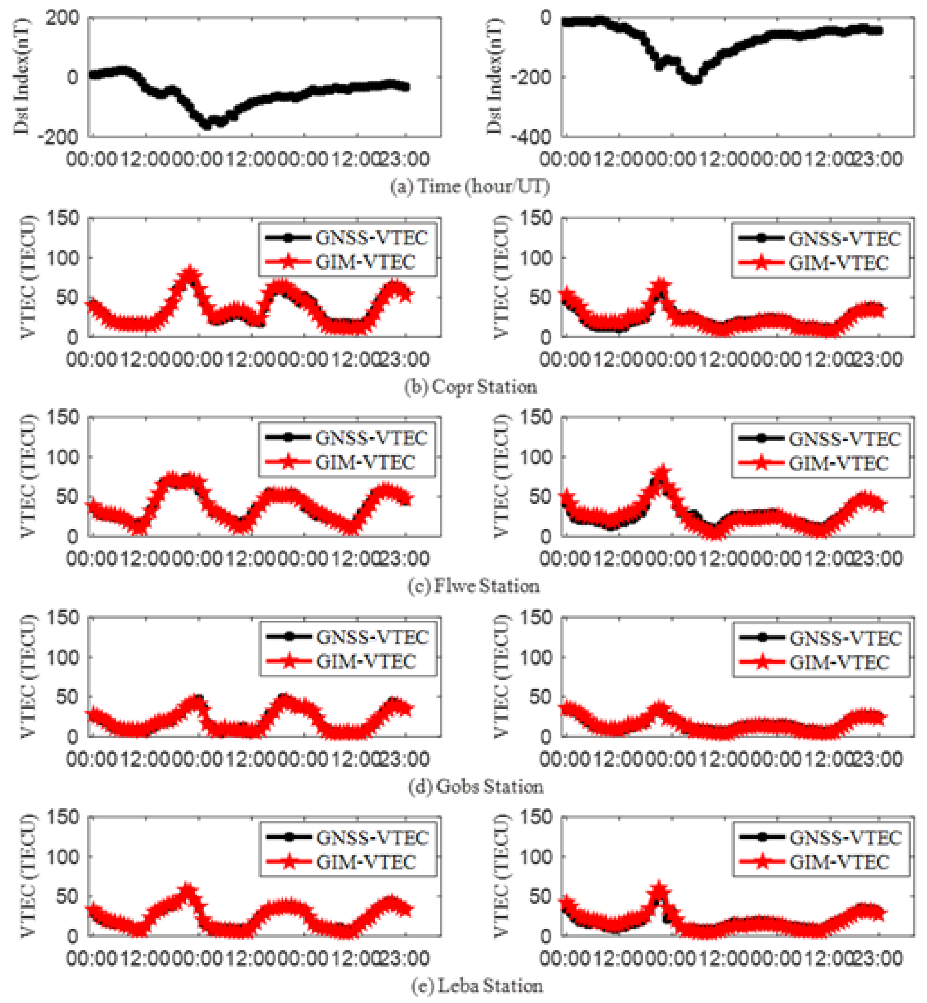
2.2. Dst and F01.7 Data
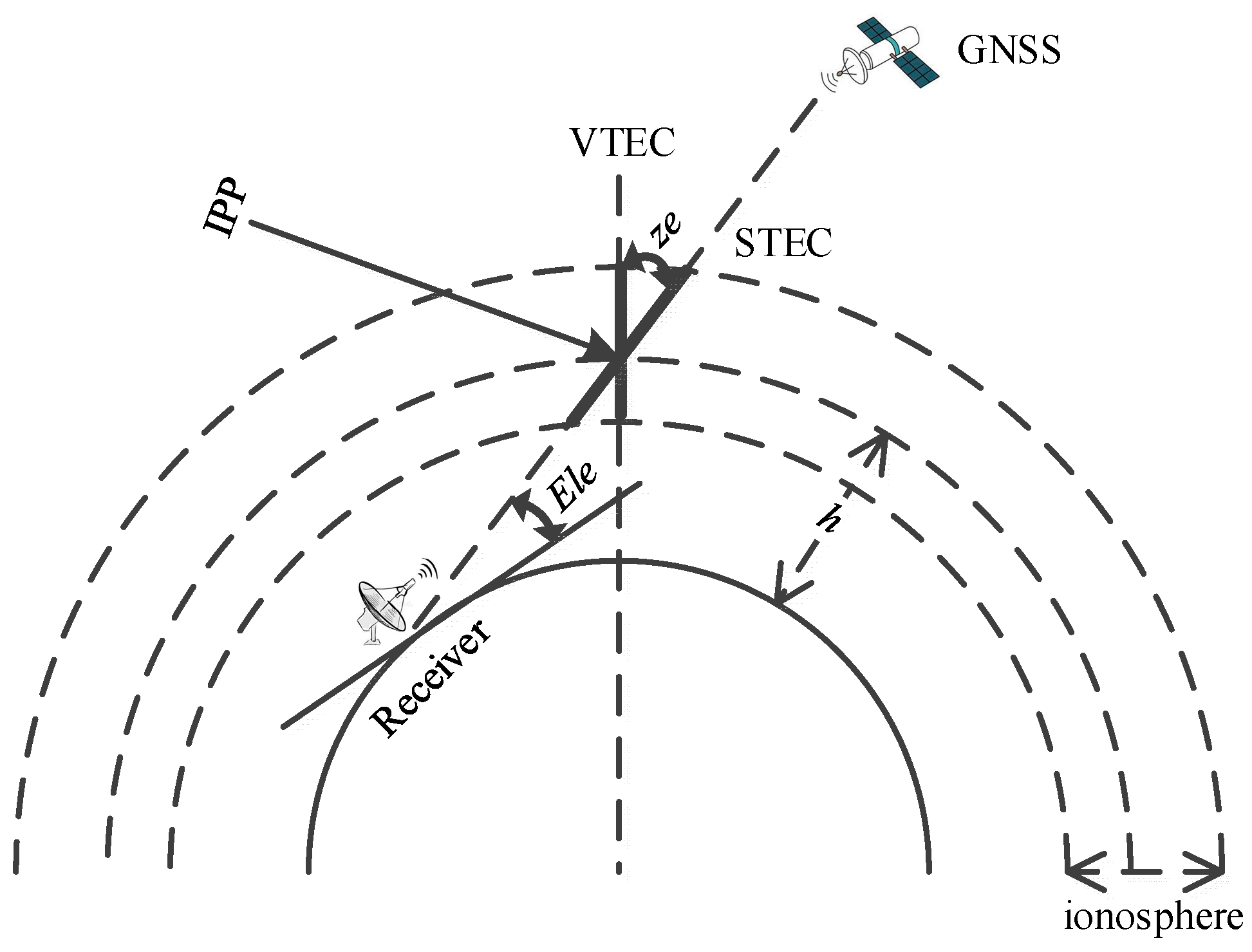
2.3. Multi-Site High-Precision Ionospheric Estimation
2.4. Gauss–Markov Kalman Filtering
2.5. Assessment Methodology
3. Results
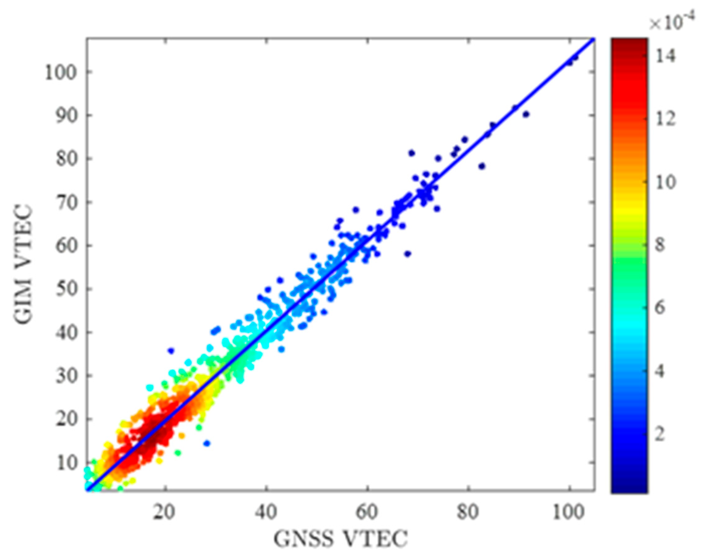
3.1. Multi-Site High-Precision Estimation Results
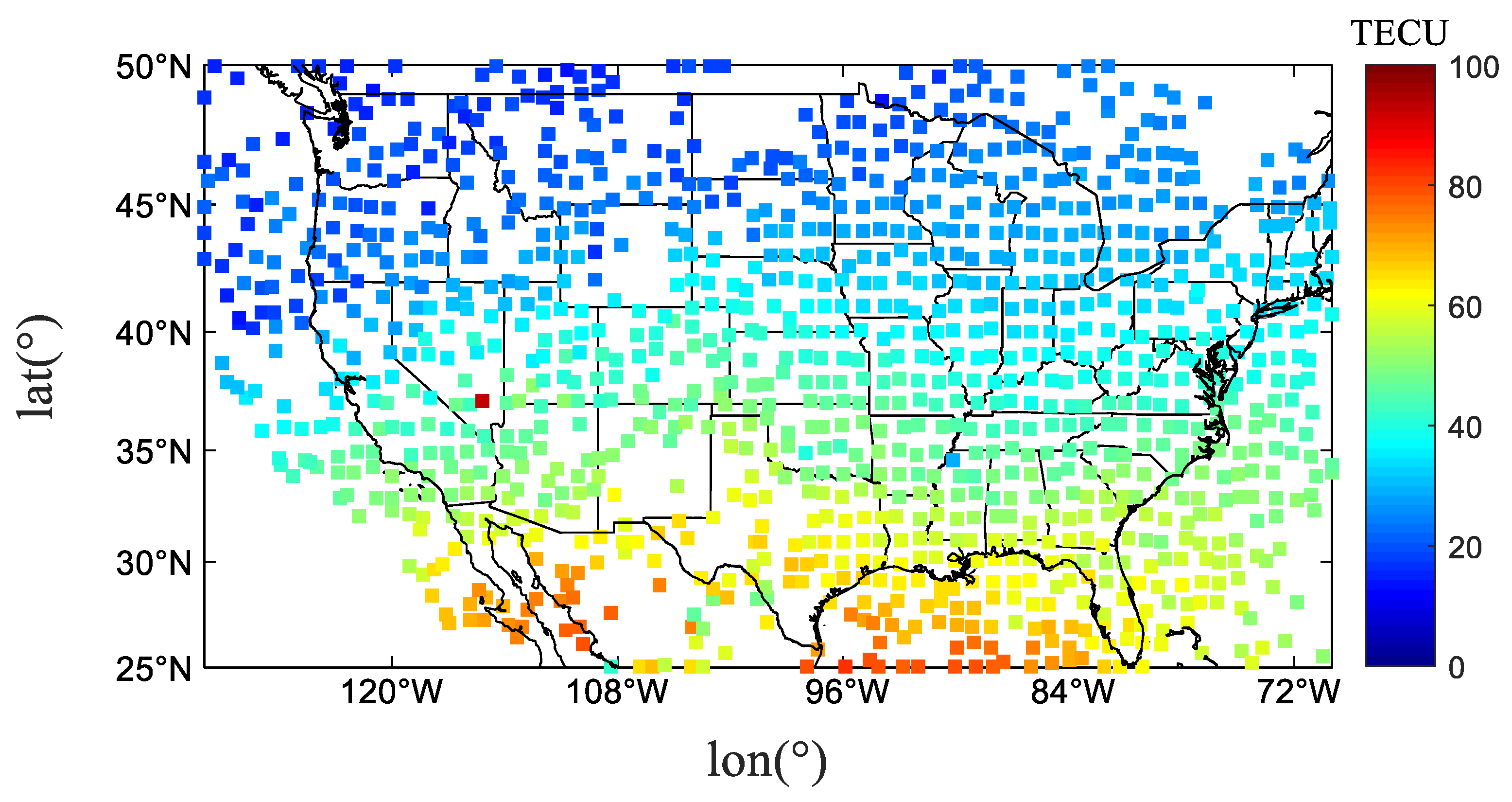
3.2. Gauss–Markov Kalman Filter Data Assimilation Results
4. Discussion
5. Conclusions
Author Contributions
Funding
Data Availability Statement
Acknowledgments
Conflicts of Interest
References
- Jin, S.; Jin, R.; Li, D. GPS detection of ionospheric rayleigh wave and its source following the 2012 Haida Gwaii earthquake. J. Geophys. Res. Space Phys. 2017, 122, 1360–1372. [Google Scholar] [CrossRef]
- Jin, S. Two-mode ionospheric disturbances following the 2005 Northern California offshore earthquake from GPS measurements. J. Geophys. Res. Space Phys. 2018, 123, 8587–8598. [Google Scholar] [CrossRef]
- Goodman, J.M. Operational communication systems and relationships to the ionosphere and space weather. Adv. Space Res. 2005, 36, 2241–2252. [Google Scholar] [CrossRef]
- Ritchie, S.E.; Honary, F. Storm sudden commencement and its effect on high-latitude HF communication links. Space Weather 2009, 7, S06005. [Google Scholar] [CrossRef]
- Ma, G.; Gao, W.; Li, J.; Chen, Y.; Shen, H. Estimation of GPS instrumental biases from small scale network. Adv. Space Res. 2014, 54, 871–882. [Google Scholar] [CrossRef]
- Cai, H.; Wang, Q. Resolving the Regional Ionospheric Grid Model by Applying Kalman Filter. In Proceedings of the China Satellite Navigation Conference (CSNC) 2016, Changsha, China, 18–20 May 2016; Volume III, pp. 425–434. [Google Scholar]
- Cooper, C.; Mitchell, C.N.; Wright, C.J.; Jackson, D.R.; Witvliet, B.A. Measurement of ionospheric total electron content using single-frequency geostationary satellite observations. Radio Sci. 2019, 54, 10–19. [Google Scholar] [CrossRef]
- Wang, H.-N.; Zhu, Q.-L.; Dong, X.; Sheng, D.-S.; Zhi, Y.-F.; Zhou, C.; Xu, B. A Novel Technique for High-Precision Ionospheric VTEC Estimation and Prediction at the Equatorial Ionization Anomaly Region: A Case Study over Haikou Station. Remote Sens. 2023, 15, 3394. [Google Scholar] [CrossRef]
- Chetia, B.; Barman, M.K.; Devi, M.; Barbara, A.K. Study of Physical and Dynamical Processes in the Ionosphere at Equatorial Anomaly Crest Region during Magnetic Storm for High and Low Solar Activity Period. In Geostatistical and Geospatial Approaches for the Characterization of Natural Resources in the Environment, Proceedings of the International Association for Mathematical Geosciences Annual Conferences, New Delhi, India, 17–20 October 2014; Springer Nature: London, UK, 2016; pp. 861–866. [Google Scholar]
- Deng, Y.; Ridley, A.J. The Global Ionosphere-Thermosphere Model and the Nonhydrostatic Processes. In Geophysical Monograph Series; Wiley: Hoboken, NJ, USA, 2014; pp. 85–100. [Google Scholar]
- Kouris, S.S.; Xenos, T.D.; Polimeris, K.V.; Stergiou, D. TEC and foF2 variations: Preliminary results. Ann. Geophys. 2004, 47, 1325–1332. [Google Scholar] [CrossRef]
- Sai Gowtam, V.; Tulasi Ram, S. Ionospheric annual anomaly New insights to the physical mechanisms. J. Geophys. Res. Space Phys. 2017, 122, 8816–8830. [Google Scholar] [CrossRef]
- Balan, N.; Liu, L.B.; Le, H.J. A brief review of equatorial ionization anomaly and ionospheric irregularities. Earth Planet. Phys. 2018, 2, 257–275. [Google Scholar] [CrossRef]
- Gan, Q.; Wang, W.; Yue, J.; Liu, H.; Chang, L.C.; Zhang, S.; Burns, A.; Du, J. Numerical simulation of the 6 day wave effects on the ionosphere: Dynamo modulation. J. Geophys. Res. Space Phys. 2016, 121, 10103–10116. [Google Scholar] [CrossRef]
- Ferdousi, B.; Raeder, J. Signal propagation time from the magnetotail to the ionosphere: OpenGGCM simulation. J. Geophys. Res. Space Phys. 2016, 121, 6549–6561. [Google Scholar] [CrossRef]
- Ridley, A.J.; Deng, Y.; Tóth, G. The global ionosphere–thermosphere model. J. Atmos. Sol.-Terr. Phys. 2006, 68, 839–864. [Google Scholar] [CrossRef]
- Bilitza, D.; Altadill, D.; Truhlik, V.; Shubin, V.; Galkin, I.; Reinisch, B.; Huang, X. International Reference Ionosphere 2016: Fromionospheric climate to real-time weather predictions. Space Weather 2017, 15, 418–429. [Google Scholar] [CrossRef]
- Wang, N.; Li, Z.; Yuan, Y.; Li, M.; Huo, X.; Yuan, C. Ionospheric correction using GPS Klobuchar coefficients with an empirical nigh-time delay model. Adv. Space Res. 2018, 63, 886–896. [Google Scholar] [CrossRef]
- Jiang, H.; Liu, J.; Wang, Z.; An, J.; Ou, J.; Liu, S.; Wang, N. Assessment of spatial and temporal TEC variations derived from ionospheric models over the polar regions. J. Geod. 2019, 93, 455–471. [Google Scholar] [CrossRef]
- Chartier, A.T.; Matsuo, T.; Anderson, J.L.; Collins, N.; Hoar, T.J.; Lu, G.; Mitchell, C.N.; Coster, A.J.; Paxton, L.J.; Bust, G.S. Ionospheric data assimilation and forecasting during storms. J. Geophys. Res. Space Phys. 2016, 121, 764–778. [Google Scholar] [CrossRef]
- Gardner, L.C.; Schunk, R.W.; Scherliess, L.; Eccles, V.; Basu, S.; Valladeres, C. Modeling the midlatitude ionosphere storm-enhanced density distribution with a data assimilation model. Space Weather 2018, 16, 1539–1548. [Google Scholar] [CrossRef]
- Mengist, C.K.; Ssessanga, N.; Jeong, S.-H.; Kim, J.-.H.; Kim, Y.H.; Kwak, Y.-.S. Assimilation of multiple data types to a regional ionosphere model with a 3D-Var algorithm (IDA4D). Space Weather 2019, 17, 1018–1039. [Google Scholar] [CrossRef]
- Tang, J.; Zhang, S.; Yang, D.; Wu, X. Assimilating GNSS TEC with an LETKF over Yunnan, China. Remote Sens. 2023, 15, 3547. [Google Scholar] [CrossRef]
- Wu, M.J.; Guo, P.; Xu, T.L.; Fu, N.F.; Xu, X.S.; Jin, H.L.; Hu, X.G. Data assimilation of plasmasphere and upper ionosphere using COSMIC/GPS slant TEC measurements. Radio Sci. 2015, 50, 1131–1140. [Google Scholar] [CrossRef]
- Zhang, H.; Tian, X. A multigrid nonlinear least squares four-dimensional Variational data assimilation scheme the with Advanced Research Weather Research and Forecasting Model. J. Geophys. Res. Atmos. 2018, 123, 5116–5129. [Google Scholar] [CrossRef]
- He, J.; Yue, X.; Hu, L.; Wang, J.; Li, M.; Ning, B.; Wan, W.; Xu, J. Observing system impact on ionospheric specification over China using EnKF assimilation. Space Weather 2020, 18, e2020SW002527. [Google Scholar] [CrossRef]
- Lin, X.; Wang, H.; Zhang, Q.; Yao, C.; Chen, C.; Cheng, L.; Li, Z. A Spatiotemporal Network Model for Global Ionospheric TEC Forecasting. Remote Sens. 2022, 14, 1717. [Google Scholar] [CrossRef]
- Kumar, S.; Veenadhari, B.; Ram, S.T.; Su, S.Y.; Kikuchi, T. Possible relationship between the equatorial electrojet (EEJ) and daytime vertical E×B drift velocities in F region from ROCSAT observations. Adv. Space Res. 2016, 58, 1168–1176. [Google Scholar] [CrossRef]
- Mungufeni, P.; Habarulema, J.B.; Migoya-Orué, Y.; Jurua, E. Statistical analysis of the correlation between the equatorial electrojet and the occurrence of the equatorial ionisation anomaly over the East African sector. Ann. Geophys. 2018, 36, 841–853. [Google Scholar] [CrossRef]
- Loewe, C.A.; Prölls, G.W. Classification and mean behavior of magnetic storms. J. Geophys. Res. 1997, 102, 14209–14213. [Google Scholar] [CrossRef]
- Ping, J.; Kono, Y.; Matsumoto, K.; Otsuka, Y.; Saito, A.; Shum, C.; Heki, K.; Kawano, N. Regional ionosphere map over Japanese islands. Earth Planets Space 2002, 54, 13–16. [Google Scholar] [CrossRef]
- Otsuka, Y.; Ogawa, T.; Saito, A.; Tsugawa, T.; Fukao, S.; Miyazaki, S. A new technique for mapping of total electron content using GPS network in Japan. Earth Planets Space 2002, 54, 63–70. [Google Scholar] [CrossRef]
- Qiao, J.; Liu, Y.; Fan, Z.; Tang, Q.; Li, X.; Zhang, F.; Song, Y.; He, F.; Zhou, C.; Qing, H.; et al. Ionospheric TEC data assimilation based on Gauss–Markov Kalman filter. Adv. Space Res. 2021, 68, 4189–4204. [Google Scholar] [CrossRef]
- Ou, M.; Fan, D.; Wang, C.; He, L. A simulation study of the Argo program-enhanced global ionospheric modeling. Adv. Space Res. 2024, 73, 1865–1874. [Google Scholar] [CrossRef]
- Aa, E.; Liu, S.; Huang, W.; Shi, L.; Gong, J.; Chen, Y.; Shen, H.; Li, J. Regional 3-D ionospheric electron density specification on the basis of data assimilation of ground-based GNSS and radio occultation data. Space Weather 2016, 14, 433–448. [Google Scholar] [CrossRef]
- Pancheva, D.; Mukhtarov, P.; Bojilova, R. Response to geomagnetic storm on 23–24 March 2023 long-lasting longitudinal variations of the global ionospheric TEC. Adv. Space Res. 2024, 73, 6006–6028. [Google Scholar] [CrossRef]
- Paul, K.S.; Haralambous, H.; Oikonomou, C. Ionospheric response of the March 2023 geomagnetic storm over European latitudes. Adv. Space Res. 2024, 73, 6029–6040. [Google Scholar] [CrossRef]
- Aa, E.; Huang, W.; Yu, S.; Liu, S.; Shi, L.; Gong, J.; Chen, Y.; Shen, H. A regional ionospheric TEC mapping technique over China and adjacent areas on the basis of data assimilation. J. Geophys. Res.-Space Phys. 2015, 120, 5049–5061. [Google Scholar] [CrossRef]
- Ou, M.; Chen, L.; Xu, N.; Zhen, W.; Chen, L. A near real-time global ionospheric data assimilation and forecast system. In Proceedings of the 2021 13th International Symposium on Antennas, Propagation and EM Theory (ISAPE), Zhuhai, China, 1–4 December 2021; pp. 1–3. [Google Scholar] [CrossRef]
- Forootan, E.; Kosary, M.; Farzaneh, S.; Schumacher, M. Empirical Data Assimilation for Merging Total Electron Content Data with Empirical and Physical Models. Surv. Geophys. 2023, 44, 2011–2041. [Google Scholar] [CrossRef]


| Storm Class | Scope |
|---|---|
| great | Dst < −350 nT |
| severe | −350 nT < Dst < −200 nT |
| strong | −200 nT < Dst < −100 nT |
| moderate | −100 nT < Dst < −50 nT |
| weak | −50 nT < Dst < −30 nT |
| Date | Copr | Flwe | Gobs | Leba |
|---|---|---|---|---|
| 23–25 March 2023 | 4.15 | 3.14 | 2.10 | 1.83 |
| 23–25 April 2023 | 4.90 | 6.27 | 2.35 | 4.23 |
| 24–26 March 2024 | 1.88 | 2.95 | 2.18 | 2.69 |
| Statistics | 3.64 | 4.12 | 2.21 | 2.92 |
Disclaimer/Publisher’s Note: The statements, opinions and data contained in all publications are solely those of the individual author(s) and contributor(s) and not of MDPI and/or the editor(s). MDPI and/or the editor(s) disclaim responsibility for any injury to people or property resulting from any ideas, methods, instructions or products referred to in the content. |
© 2025 by the authors. Licensee MDPI, Basel, Switzerland. This article is an open access article distributed under the terms and conditions of the Creative Commons Attribution (CC BY) license (https://creativecommons.org/licenses/by/4.0/).
Share and Cite
Wang, H.-N.; Zhu, Q.-L.; Dong, X.; Ou, M.; Zhi, Y.-F.; Xu, B.; Zhou, C. A Regional Ionospheric TEC Map Assimilation Method Considering Temporal Scale During Geomagnetic Storms. Remote Sens. 2025, 17, 951. https://doi.org/10.3390/rs17060951
Wang H-N, Zhu Q-L, Dong X, Ou M, Zhi Y-F, Xu B, Zhou C. A Regional Ionospheric TEC Map Assimilation Method Considering Temporal Scale During Geomagnetic Storms. Remote Sensing. 2025; 17(6):951. https://doi.org/10.3390/rs17060951
Chicago/Turabian StyleWang, Hai-Ning, Qing-Lin Zhu, Xiang Dong, Ming Ou, Yong-Feng Zhi, Bin Xu, and Chen Zhou. 2025. "A Regional Ionospheric TEC Map Assimilation Method Considering Temporal Scale During Geomagnetic Storms" Remote Sensing 17, no. 6: 951. https://doi.org/10.3390/rs17060951
APA StyleWang, H.-N., Zhu, Q.-L., Dong, X., Ou, M., Zhi, Y.-F., Xu, B., & Zhou, C. (2025). A Regional Ionospheric TEC Map Assimilation Method Considering Temporal Scale During Geomagnetic Storms. Remote Sensing, 17(6), 951. https://doi.org/10.3390/rs17060951