The Paradigm Shift in Hyperspectral Image Compression: A Neural Video Representation Methodology

Abstract

In recent years, with the continuous development of deep learning, the scope of neural networks that can be expressed is becoming wider and their expressive ability stronger. Traditional deep learning methods based on extracting latent representations have achieved satisfactory results. However, in the field of hyperspectral image compression, the high computational cost and the degradation of their generalization ability reduce their application. We analyze the objective formulation of traditional learning-based methods and draw the conclusion that rather than treating the hyperspectral image as an entire tensor to extract the latent representation, it is preferred to view it as a stream of video data, where each spectral band represents a frame of information and variances between spectral bands represent transformations between frames. Moreover, in order to compress the hyperspectral image of this video representation, neural video representation that decouples the spectral and spatial dimensions from each other for representation learning is employed so that the information about the data is preserved in the neural network parameters. Specifically, the network utilizes the spectral band index and the spatial coordinate index encoded with positional encoding as its input to perform network overfitting, which can output the image information of the corresponding spectral band based on the index of that spectral band. The experimental results indicate that the proposed method achieves approximately a 5 dB higher PSNR compared with traditional deep learning-based compression methods and outperforms another neural video representation method by 0.5 dB when using only the spectral band index as input.

1. Introduction

In recent years, with the continuous improvement in satellite and airborne equipment, the acquisition of hyperspectral imagery has become more convenient and efficient. Compared with traditional RGB images, hyperspectral images provide more detailed and multi-dimensional data by capturing spectral information in multiple bands. This type of image has rich spectral resolution and is able to capture details that are not visible to the naked eye; thus, it has great potential for applications in resource exploration [1], environmental monitoring [2], agricultural assessment [3], urban planning [4], and disaster monitoring [5]. However, such high-dimensional spectral information presents technical challenges, especially in data transmission and storage. For real-time applications such as satellite communications [6] and unmanned aerial remote sensing [7], the large data volume of hyperspectral images and the increasing costs of transmission and storage make the efficient compression of these images a key issue in current research.

Traditional image compression methods such as JPEG [8], JPEG2000 [9], BPG [10], etc., have performed well in compressing ordinary RGB images, especially in achieving a certain balance between the visual effect and computational efficiency. However, when it comes to compressing hyperspectral images, these methods have significant limitations. Each band of hyperspectral imagery not only contains rich spatial information but also has strong spectral correlation with different bands. Traditional compression methods cannot effectively capture this spectral correlation, resulting in the loss of a large amount of effective information in the compression process. As a result, they cannot meet the high data compression quality requirements of hyperspectral imaging applications.

In addition, in some specific applications, the compression of hyperspectral images requires near-lossless or lossless compression, and methods capable of achieving this, such as CCSDS123.0-b-2 [11] and other standards, have shown satisfactory results. By fine-tuning the quantization process, these methods are able to achieve high compression ratios while maintaining data quality. However, as high time costs limit their application, researchers have gradually turned their attention to how to achieve effective lossy compression.

In recent years, research on lossy image compression has made significant progress. For natural images, Ballé et al. [12] pioneered an end-to-end image compression framework and developed a hyper-priori model to eliminate the spatial redundancy among pixels. However, with the increasing compression performance requirements of real-world applications, the traditional architecture struggles to meet the demand. To this end, researchers have explored various directions of improvement. These include designing more powerful encoder–decoder networks to enhance the representation ability of features or introducing more advanced likelihood modelling methods into the super-priori model to optimize the coding rate. The exploration of these directions has contributed to the rapid development of natural image compression.

In the field of remote sensing image compression, researchers usually build on the successful experience of natural image compression techniques. At the same time, they optimize and research the unique properties of remote sensing images to adapt methods to their characteristics, such as high resolution and rich spatial details. Although these methods have achieved some success in compressing remote sensing images, it is often difficult to achieve the expected results by directly applying natural image compression methods to hyperspectral images. This is due to the higher complexity and unique spectral properties of the latter. This challenge has motivated researchers to develop more refined compression schemes for the characteristics of hyperspectral images.

A hyperspectral image consists of multiple bands, each of which can be viewed as a two-dimensional image with specific spectral information. These images are arranged in spectral dimensions to form a three-dimensional data cube. In practice, the data transmission of hyperspectral imagery is usually performed in a format similar to video streaming. This is because band data are often processed and delivered sequentially during transmission, a structure that is very similar to the temporal relationship between frames in a video stream. Therefore, the relationship between spectral bands in hyperspectral images can be mapped to the conversion between frames in a video stream.

The efficient representation of hyperspectral imagery can be achieved in a similar way by introducing a neural video representation based on neural radiation fields (NeRFs) [13]. NeRFs show great potential for modeling complex data with continuous spatial and temporal variations due to their high fitting capability and flexibility. Recent studies have shown that the NeRF framework has achieved significant results in 3D scene reconstruction [14] and video representation [15,16]. This provides important insights for the efficient processing of hyperspectral images.

In this study, starting from the spectral characteristics of hyperspectral images themselves and introducing the mapping relationship in video representation, an innovative modelling and compression method for hyperspectral images is proposed. This method provides a new solution for efficient data representation. The main contributions are detailed below:

• A framework for the video-based processing of hyperspectral images

We innovatively consider hyperspectral images to be a form of data similar to video streaming for efficient network-based processing. Two video stream partitioning methods are proposed: single-channel video stream and three-channel video stream. The former treats each spectral band as an independent frame, which can capture the small variations between spectra in a fine-grained way; the latter combines adjacent bands into pseudo-RGB frames, which achieves a better trade-off between coding efficiency and storage space;

2.

Hyperspectral image modelling based on neural video representation

We use neural video representation to efficiently model hyperspectral images and analyze in detail the influence of the input form on the modelling effect. Experiments show that it is difficult to reconstruct high quality images by using only spectral indices (band order numbers) as input. Therefore, we propose combining spectral indices with the 2D spatial coordinates of pixels as the neural network inputs, which enhances the ability to capture spatial features and accurately model complex correlations between spectral bands. In this framework, the information of hyperspectral images is effectively embedded in the network parameters. This allows for efficient image compression and storage;

3.

Experimental Validation and Performance Evaluation

The effectiveness and applicability of the proposed method in hyperspectral image compression are verified with a large number of experiments. The experimental results show that the proposed neural video representation method is able to achieve excellent performance in the PSNR, MS-SSIM, and SAM metrics, which further improves compression efficiency while preserving image quality compared with traditional methods. This result demonstrates the potential of the method in practical applications and opens up new possibilities for the efficient transmission and storage of hyperspectral images.

The rest of this paper is structured as follows: In Section 2, we review related work on deep learning-based natural image compression methods, remote sensing image compression methods, and hyperspectral image compression methods. In Section 3, we analyze the shortcomings of the learning-based methods and describe the proposed FIO-F and JSCIFI-F models in detail. In Section 4, we present experimental results and analyses to evaluate the performance of the proposed method. Finally, in Section 5, we conclude this paper with an outlook on future research directions.

2. Related Work

In this section, we first introduce deep learning-based natural image compression methods and remote sensing image compression methods and analyze their limitations in hyperspectral image compression. Then, the existing hyperspectral image compression methods are discussed in detail.

2.1. Deep Learning-Based Compression Methods for Natural and Remote Sensing Images

Traditional image compression methods (e.g., JPEG [8] and JPEG2000 [9]) mainly rely on classical transform coding techniques, such as discrete cosine transform (DCT [17]) or discrete wavelet transform (DWT [18]), and then perform the quantization and entropy coding of the transform coefficients to achieve compression.

These methods were originally designed primarily for the compression of natural images, relying on hand-crafted rules and predetermined transformation strategies.

However, with the increase in image complexity and the demand for higher compression rates and quality, the limitations of these traditional methods have gradually become apparent.

In contrast, learning-based image compression methods use an end-to-end deep learning framework to automatically learn feature extraction and compression laws from data. These methods typically construct encoders by stacking convolutional blocks, which are used to extract latent feature representations of the input image.

These latent representations exhibit a high degree of density and representational power by capturing the spatial structure and content information of the image through the encoder.

After obtaining the latent representations, these methods model them by using entropy models. Entropy models typically assume that the distribution of the latent representation is Gaussian (or mixed Gaussian) and model it by introducing a learnable prior distribution. This approach allows the latent representation to be reconstructed more accurately in the decoding stage, while significantly improving compression efficiency.

He et al. [19] proposed a spatial channel context adaptive model by combining the inhomogeneous group entropy model with the context model, which successfully solved the problem of reusing channels with low entropy distribution. Liu et al. [20] proposed a parallel Transformer–CNN hybrid module, which combines the local modelling capability of CNNs and the non-local modelling capability of Transformers and optimizes the codec to optimize and solve the spatial redundancy problem of natural images in the compression process. Fu et al. [21] proposed a more flexible discrete Gaussian–Laplace Logistic Mixed Model (GLLMM), which can more accurately and efficiently adapt to different content in different images and regions with the same complexity.

On the other hand, for remote sensing images, Shao et al. [22] used the discrete wavelet transform (DWT) to divide the image features into high-frequency and low-frequency feature components, they also introduced a frequency domain coding–decoding module to improve the ability of the model to represent the high-frequency and low-frequency features.

Zhang et al. [23] proposed a method of using diffusion models through ground stations to solve the problem of information loss that may occur in the compressed remote sensing satellite images. The problem of information loss in remote sensing satellite images after compression is solved by deploying a diffusion model at the ground station.

However, although the above methods have achieved excellent performance in natural and remote sensing image compression, they face certain challenges in hyperspectral image compression. The spectral information represented by each band (or channel) of hyperspectral images has large differences, and the importance of each channel is not the same, which makes some compression techniques (e.g., the spatial channel context adaptive model) for natural images not fully applicable to hyperspectral images. On the other hand, although the combined module of a CNN and a Transformer shows significant ability in feature extraction, in hyperspectral images, due to their large data volume and complex spectral information, the direct introduction of a high-complexity Transformer model may lead to the overall computational complexity being too high and the number of model parameters being too large, which in turn affects the efficiency of training and inference.

In addition, traditional high-frequency and low-frequency feature division methods (e.g., DWT) and image post-processing techniques based on diffusion models, although effective in the compression of other types of images, are less applicable to hyperspectral images due to the specificity of their spectral information and spatial structure. Therefore, specific compression techniques for hyperspectral images need to be developed to better process their complex spectral and spatial characteristics.

2.2. Deep Learning-Based Hyperspectral Image Compression Method

Verdu et al. [24] proposed a channel clustering strategy, which effectively simplifies the complexity of processing a large number of bands by reducing the computational requirements and shows good adaptability. However, the method is only applicable to hyperspectral image compression in a small number of bands, and it fails to effectively deal with the interspectral redundancy problem, which limits its application to hyperspectral images.

Guo et al. [25] designed an edge-guided hyperspectral compression network, which significantly improves the structure and detail preservation of images by capturing edge features. However, due to the overall compression of 50-band hyperspectral images, there are shortcomings in the extraction of interspectral information, and the network fails to fully explore the correlation between bands.

Martin et al. [26] proposed a Transformer-based autoencoder for pixel-level hyperspectral image compression by modeling remote spectral dependencies. Although the method effectively leverages the interspectral correlation between adjacent bands, the spatial redundancy treatment of single-band images is weak, which affects spatial information compression efficiency.

Afsana et al. [27] introduced three-dimensional convolution into a hyperspectral image compression encoder, which can eliminate spatial redundancy and retain spectral information to some extent. However, the high computational complexity and the large number of model parameters of this method limit its application in resource-constrained scenarios.

Considering the shortcomings of the existing hyperspectral image compression and modelling methods, the core idea of neural video representation is introduced into the spectral segment modelling of hyperspectral images, which captures the corresponding relationship between spectral segments by using neural networks to jointly model the spectral correlation and spatial properties and at the same time better preserves the key information of the image in the compression process.

To present the results more clearly, we have summarized them in Table 1.

Table 1. Brief summary of methods in related work section.

Method	Advantages	Disadvantages	Applicability	Limitations	Performance Indicators
He et al. (2022) [19]	Enables efficient channel reuse	Less effective for hyperspectral images	Natural images	Not fully applicable to hyperspectral images	Improved compression efficiency
Liu et al. (2023) [20]	Combines a CNN and Transformer for optimal spatial redundancy reduction	High computational complexity	Natural images	High model parameter count	High compression rates
Fu et al. (2023) [21]	Adapts dynamically to image content with GLLMM	Complex model structure	Natural images	Model adaptability	Enhanced adaptability
Shao et al. (2024) [22]	Improved high-frequency and low-frequency feature representation	Frequency domain techniques may not suit hyperspectral images	Remote sensing images	Limited application in hyperspectral images	Enhanced feature representation
Zhang et al. (2024) [23]	Mitigates information loss using diffusion models at ground stations	Dependent on infrastructure	Remote sensing satellite images	Computational and infrastructural dependency	Loss minimization
Verdu et al. (2023) [24]	Reduces computational requirements through channel clustering	Inefficient for large band numbers	Small-band hyperspectral images	Interspectral redundancy handling is limited	Complexity reduction
Guo et al. (2022) [25]	Enhances structure and detail preservation with edge-guided features	Weak interspectral information extraction	General hyperspectral images	Limited correlation exploration between bands	Improved edge preservation
Martin et al. (2024) [26]	Captures interspectral dependencies effectively	Suboptimal spatial compression	Hyperspectral images with adjacent bands	Weak handling of single-band spatial redundancy	Enhanced spectral modeling
Afsana et al. (2024) [27]	Utilizes 3D convolutions for better spectral retention	High computational resource needs	Resource-rich environments	Unsuitable for resource-constrained scenarios	Spectral retention

3. Proposed Methods

3.1. The Necessity of a Paradigm Shift in Hyperspectral Image Compression

As mentioned before, there are significant issues when compressing hyperspectral remote sensing images by using traditional deep learning methods. Below, we will attempt to theoretically analyze the reasons behind these problems to the best of our ability.

Problem (1): the currently available open-source datasets for hyperspectral images are insufficient to support deep learning models in extracting generalized features;

Problem (2): the excessively high number of spectral channels in hyperspectral images limits the performance of convolutional neural networks;

Problem (3): the optimization objectives of traditional deep learning-based compression methods partially lose their effectiveness.

We provide the classical compression pipeline of deep learning-based methods:

$$\underset{{\mathrm{\Theta }}_1+{\mathrm{\Theta }}_2}{\arg \min }L=\lambda \left|\left|x-{\mathcal{F}}_{{\mathrm{\Theta }}_2}({\mathcal{F}}_{{\mathrm{\Theta }}_1}\left(x\right))\right|\right|+\mathcal{R}\left({\mathcal{F}}_{{\mathrm{\Theta }}_1}\left(x\right)\right)$$

(1)

We denote the reconstructed image by $\widehat{x}={\mathcal{F}}_{{\mathrm{\Theta }}_2}({\mathcal{F}}_{{\mathrm{\Theta }}_1}\left(x\right))$ and the latent feature by $\widehat{y}={\mathcal{F}}_{{\mathrm{\Theta }}_1}\left(x\right)$. Naturally, ${\mathrm{\Theta }}_1$ and ${\mathrm{\Theta }}_2$ denote the encoder parameters and decoder parameters, respectively. $\lambda$ denotes the Lagrange coefficient controlling the compression ratio, and $\mathcal{R}$ represents the function (typically the Shannon entropy equation) calculating the compression ratio whose input is the latent feature from the input images. For an enhanced representation capability (namely, dense in this scenario) of the feature space, the transformed features are further constrained with a multilayer Gaussian likelihood as follows:

$$p\left(\widehat{y}\right)~{\displaystyle \sum }_{k=1}^K{\omega }^{\left(k\right)}\mathcal{N}\left({\mu }^{\left(k\right)},{\sigma }^{2\left(k\right)}\right)$$

(2)

In some works, the side information $\widehat{z}=\mathcal{Q}\left(\widehat{y}\right)$ is inserted to indicate $p\left(\widehat{y}\right)$ as $p_{\widehat{y}|\widehat{z}}(\widehat{y}|\widehat{z})$. However, as this will not affect the analytical results, we will not implement it.

Here, we assume that batch optimization can achieve similar effects to overall optimization. In fact, in the field of computer vision, the former is more feasible in most cases and tends to achieve better generalization. Further, considering an input dataset consisting of $N$ images, $x=\left[x_1,x_2,\dots ,x_N\right]$, Formulation (1) can be further transformed into the following form:

$$\begin{array}{l}\underset{{\mathrm{\Theta }}_2}{\min }\left|\left|x-{\mathcal{F}}_{{\mathrm{\Theta }}_2}\left(Y\right)\right|\right|\\ \mathrm{s}.\mathrm{t}. Y\in \underset{{\mathrm{\Theta }}_1}{\min }\mathcal{R}\left({\mathcal{F}}_{{\mathrm{\Theta }}_1}\left(x\right),\lambda \right)\end{array}$$

(3)

Feature $Y$ plays a key role in this optimization objective. Both ${\mathcal{F}}_{{\mathrm{\Theta }}_2}\left(\cdot \right)$ and the feasible domain of $Y$ determine the compression performance.

For Problem (1):

It has been provided that the expected loss $L\left({\mathrm{\Theta }}_1+{\mathrm{\Theta }}_2\right)$ has the following relationship with the empirical loss: $\widehat{L}\left({\mathrm{\Theta }}_1+{\mathrm{\Theta }}_2\right)$ [28,29], so we will not provide further discussion.

$$L\left({\mathrm{\Theta }}_1+{\mathrm{\Theta }}_2\right)\le \widehat{L}\left({\mathrm{\Theta }}_1+{\mathrm{\Theta }}_2\right)+2{\mathcal{R}}_N\left(\cdot \right)+\mathcal{O}\left({\displaystyle \frac{1}{\sqrt{N}}}\right)$$

(4)

${\mathcal{R}}_N\left(\cdot \right)$ reflects the maximum potential variability of the loss through random variables in the parameter space. From a heuristic perspective, the feasible domain of $Y$ cannot reflect the pattern of the compression task when input images are limited, so this transforms it into a simple pattern matching task.

For Problem (2):

Under the condition of a fixed generalization error, the sample complexity of the model, i.e., the minimum number of required samples, is exponentially related to the dimensionality of the feature space. To enable the model to learn similar statistical information from the data, the number of data points must be increased.

For example, to achieve the distortion of $ϵ$, the number of training items required is as follows [29,30,31]:

$$N^{*}=\mathcal{O}\left({\displaystyle \frac{\mathcal{O}\left(k^{2}CI\right)+\log \left(\frac{1}{\delta }\right)}{{ϵ}^2}}\right)$$

(5)

$\delta$ is a probability tolerance parameter; specifically, it is the acceptable probability of generalization failure, i.e., the proportion of likelihood by which our expected generalization performance may deviate. $k$ denotes the kernel size of the CNN, $C$ denotes the number of CNN kernels, and $I$ denotes the input channel. Typically, $C$ is several times larger than $I$; here, we assume that $C=kI$. Then, we have

$$N^{*}=\mathcal{O}\left({\displaystyle \frac{\mathcal{O}\left(k^3{I}^2\right)+\log \left(\frac{1}{\delta }\right)}{{ϵ}^2}}\right)$$

(6)

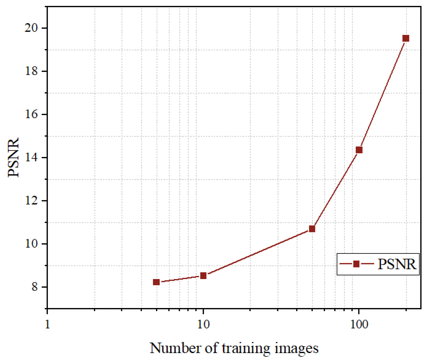
It can be observed that as the number of input channels increases, the required size of the training dataset increases quadratically, and the existing open-source hyperspectral datasets fall far short of the training requirements.

In this example, by using an RGB dataset, we randomly selected a certain number of data points and trained the model multiple times to obtain an average, resulting in the curve shown in Figure 1. (The testing images are not included in any training set).

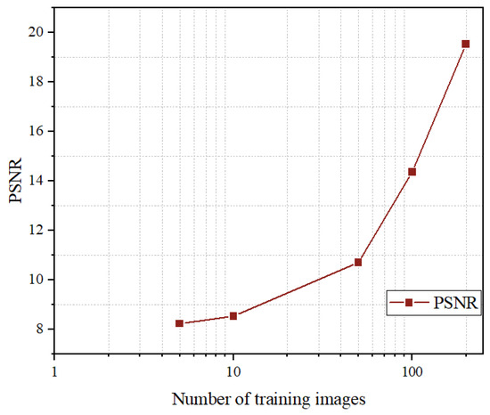
Figure 1. The variance in the PSNR on different number of training images using the method of Pan et al. [32] (the bpp setting is over 0.5 bpp).

For Problem (3):

As discussed in Problem (1) and Problem (2), the learning-based method is not realistic for the hyperspectral image compression scenario; therefore, we consider employing the index to replace the learning process towards latent features. In other words, we cut down the constraints of Formulation (3) and transform the feature domain learning task into an index-to-pixel learning task. Instead of employing significant computational resources to learn feature dependencies in high-dimensional hyperspectral image data, we prefer to learn a simpler task at a much lower cost, even though this task may not yet possess generalizability.

The formulation of the index-to-pixel learning task is as follows:

$$\begin{array}{l}\underset{{\mathrm{\Theta }}_2}{\min }\left|\left|x-{\mathcal{F}}_{{\mathrm{\Theta }}_2}\left(\Xi \right)\right|\right| \\ \mathrm{s}.\mathrm{t}. {\mathrm{\Theta }}_2\in Size\left({\mathrm{\Theta }}_2\right) \end{array}$$

(7)

This is easier to train because the term of $Size\left({\mathrm{\Theta }}_2\right)$ and the index $\Xi$ can be a constant when the input and the compression ratio are deterministic.

We compare the complexity of Formulations (3) and (7) when compressing $N$ images (assume the required images are satisfied and each image is with the shape of $\left(I,W,H\right)$):

$$\begin{array}{c} \underbrace{\mathcal{O}\left(\underset{c\mathrm{ontained} \mathrm{in} \mathrm{network} \mathrm{itself}}{\underbrace{k^2{C}^2{I}^{2}WH}}\cdot \underset{\mathrm{contained} \mathrm{in} \mathrm{training}}{\underbrace{NWH}}\right)}\\ \mathrm{formulation} \left(3\right)\end{array} \mathrm{with} \begin{array}{c}\underbrace{\mathcal{O}\left(N\Xi \log \left(\Xi \right)\right)}\\ \mathrm{formulation} \left(7\right)\end{array}$$

(8)

In NeRF-based methods such as FHNeRF, $\Xi$ is the spatial domain; therefore, Formulation (7) has only the complexity of $\mathcal{O}\left(NWH\log \left(WH\right)\right)$ compared with the classical compression pipeline of deep learning-based methods denoted as Formulation (3).

3.2. The Processes of the Proposed Method

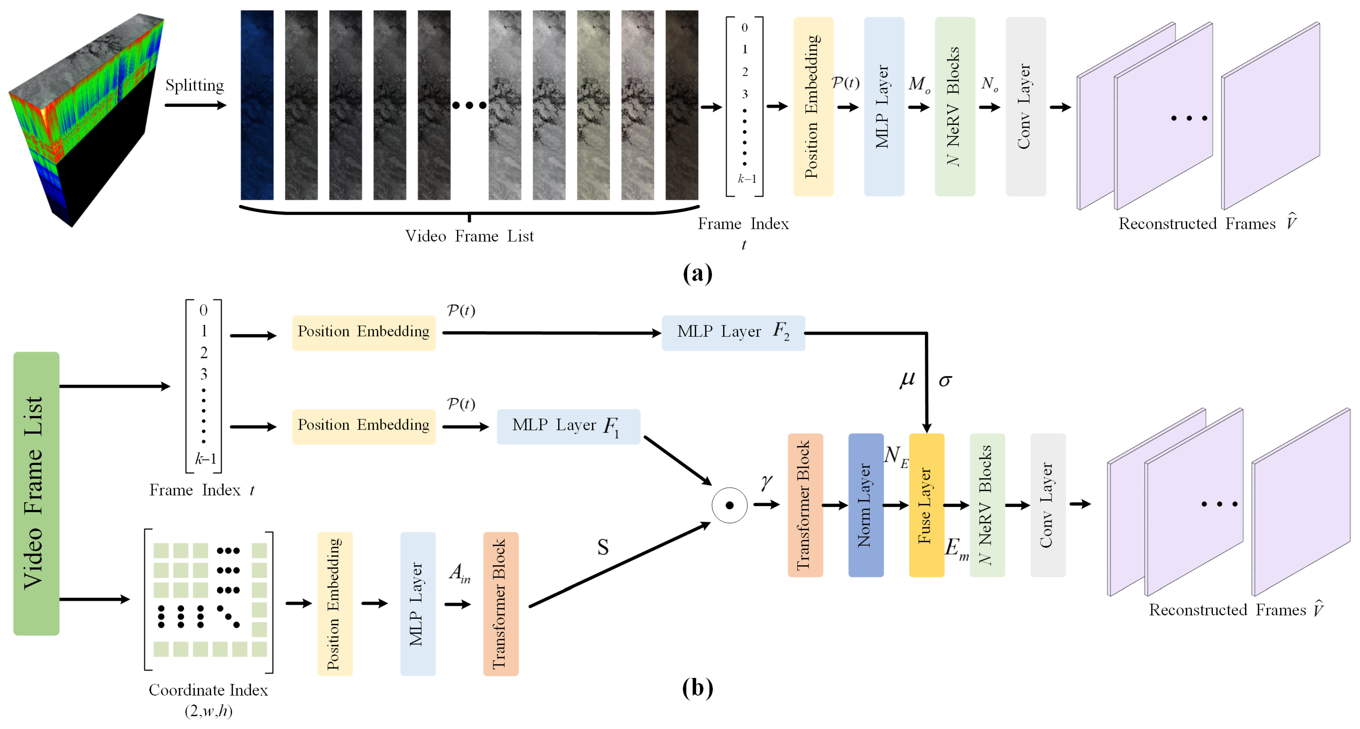
The overall framework of the proposed method is illustrated in Figure 2b, where a framework of a joint spatial coordinate index with a frame index is adopted.

Figure 2. Video-based hyperspectral image compression framework. (a) Frame-index-only framework (FIO-F). (b) Joint spatial coordinate index with frame index framework (JSCIFI-F). MLP denotes the multilayer perceptron.

In Figure 2a, hyperspectral image $I$ is first segmented into k three-channel tensors, which can be grouped into a list as $V=\left[v_0,v_1,v_2,\dots ,v_{k-1}\right]$. Then, according to the theory of NeRV [15], $V$ can be represented by a neural network $f_{\theta }:{ℝ}^1\to {ℝ}^{3\times W\times H}$, where the input of $f_{\theta }$ is frame index t, and the output is the corresponding frame, namely the three-channel image. Based on this, the storage capacity taken by the neural network parameters represents the size of the compressed hyperspectral image. For the classical deep learning-based compression issue, $Loss=R+\lambda D$, the optimization of $R$ is then decoupled from the loss function, and the neural network only needs to learn how to use a predetermined number of parameters to learn how to recover a higher-quality image output. To achieve interdomain conversion, the frame index number needs to be positionally encoded, because directly feeding the parameters into the network for overfitting training does not achieve satisfactory results [16,21]. Specifically, the position encoding in [33] is employed:

$$\mathcal{P}\left(t\right)=\left(\sin \left(b^0\pi t\right),\cos \left(b^0\pi t\right),\dots ,\sin \left(b^{l-1}\pi t\right),cos\left(b^{l-1}\pi t\right)\right)$$

(9)

where $b$ and $l$ are pre-defined hyperparameters. $t$ is the normalized input between [0, 1] using the max number of indexes.

$\mathcal{P}\left(t\right)$ is then input into the following network architecture to abtain the fitting function. This can be formulated as follows:

$$M_o=MLP\left(\mathcal{P}\left(t\right)\right)$$

(10)

$$N_o=NeR{V}_{N-1}\left(\cdot \cdot \cdot \left(NeR{V}_0\left(M_o\right)\right)\right)$$

(11)

$${\widehat{v}}_t=Conv\left(N_o\right)$$

(12)

where ${\widehat{v}}_t$ denotes the reconstructed t-th frame, and $N_o$ is generated by using N NeRV blocks. Then, the final output $\widehat{V}$ can be characterized as follows:

$$\widehat{V}=Concat\left({\widehat{v}}_0,{\widehat{v}}_1,\dots {\widehat{v}}_{k-1}\right)$$

(13)

where $Concat\left(\cdot \right)$ is the concatenate operation for the channel dimension.

In Figure 2b, the input of JSCIFI-F employs the same input $V$ with FIO-F. However, since FIO-F directly employs the frame index to directly obtain the full spatial–temporal information of hyperspectral image $I$, this leads to parameter redundancy in the setup of the network architecture, which fails to achieve a more compact information representation. Therefore, in JSCIFI-F, the input is decomposed into temporal and spatial contexts for separate coding to achieve more compact parameter learning. The embedding $E_m$ generation process of JSCIFI-F can be formulated as follows:

$$\gamma =F_1\left(\mathcal{P}\left(t\right)\right)\odot \mathrm{S}$$

(14)

$$E_m=F_{fuse}\left(\gamma ,F_2\left(\mathcal{P}\left(t\right)\right)\right)$$

(15)

where $F_{fuse}$ denotes a feature extraction network with a mixture of a transformer block and an MLP block, and $F_1$ and $F_2$ are MLP layers with fewer parameters which output a d-dimensional vector. $\mathrm{S}$ is a spatial context embedding with a size of $\left[d\times h\times w\right]$. The position embedding is decomposed into a temporal vector, $F\left(\mathcal{P}\left(t\right)\right)$, and a spatial vector, $\mathrm{S}$. Finally, a feature fusion layer is adopted to fuse the spatial and temporal vectors into the position embeddings. To enable vector $\mathrm{S}$ to contain the spatial information, the same position encoding with FIO-F is adopted; then, a transformer layer with single-head attention is adopted for feature extraction. The process can be formulated as

$$A_{in}=MLP\left(Concat\left(\mathcal{P}\left(x\right),\mathcal{P}\left(y\right)\right)\right)$$

(16)

$$\mathrm{S}=\mathrm{TF}\left(A_{in}\right)$$

(17)

The x and y dimensions of the coordinates are first encoded separately and are then concatenated before the MLP layer and transformer layer $\mathrm{TF}$. Differences in spatial information between different hyperspectral images are determined with different coding network parameters.

After disentangling and the feature fusion process, $E_m$ is finally used to reconstruct the output image. The encoding of the temporal information is extracted by an additional edge network and fused with the embedding, and the fused feature is finally input into the NeRV blocks to generate $\widehat{V}$.

For either architecture, the loss function contains only a D term, unlike previous deep learning compression frameworks.

$$Loss=D\left(\widehat{V},V\right)$$

(18)

$$={\displaystyle \frac{1}{k}}{\displaystyle \sum }_{i=0}^{k-1}MSE\left({\widehat{v}}_i,v_i\right)$$

(19)

where $MSE\left(\cdot \right)$ denotes the Mean Square Error (MSE).

The proposed method is the same as FHNeRF [34], decoupling the computation of rates in the rate-distortion loss function and allowing for network quality improvement.

3.3. Detailed Construction of Network Architecture

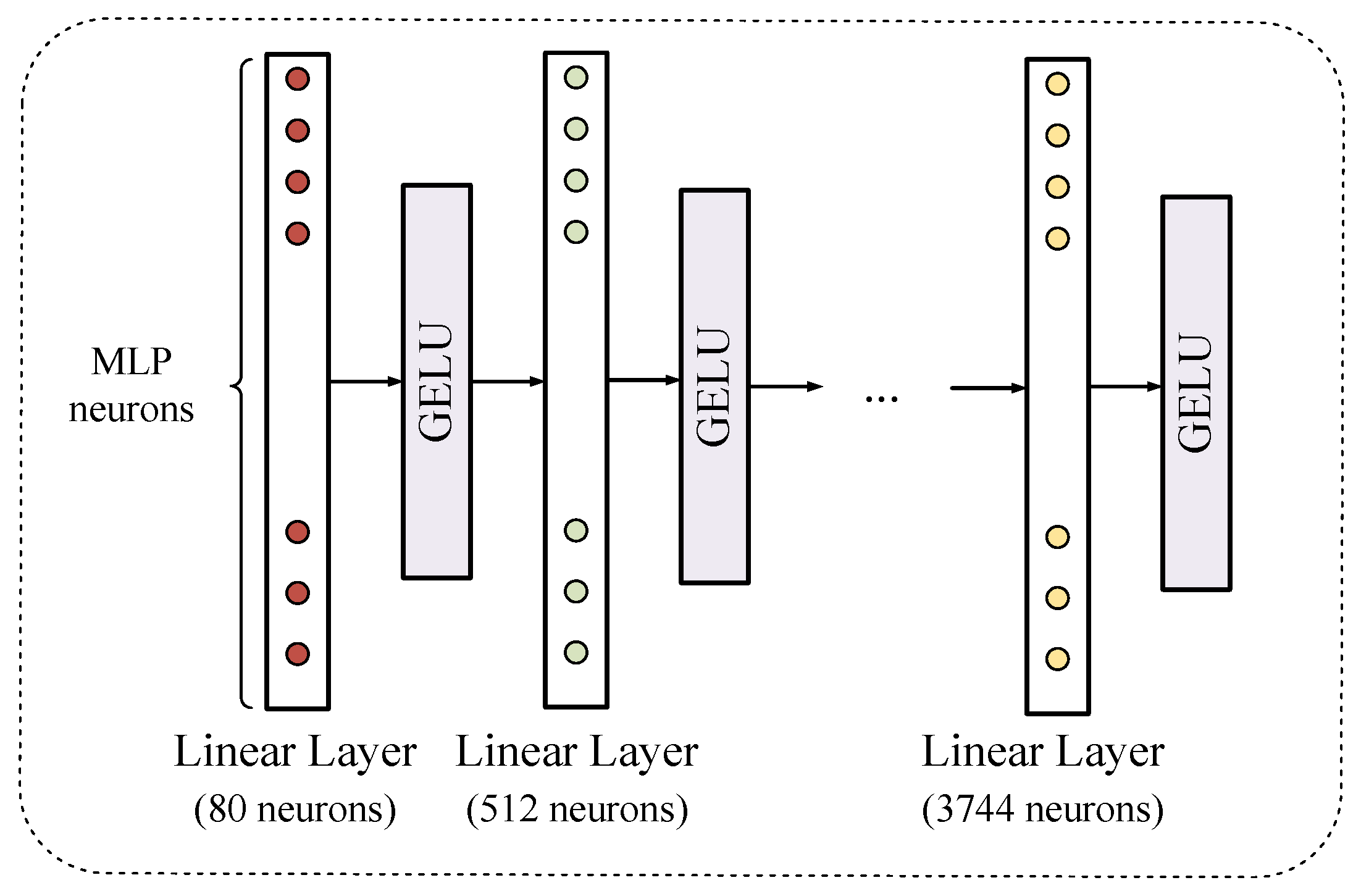
The MLP layer is illustrated in Figure 3. It converts the input encoded position vector into a feature tensor and usually contains a collection of several linear and activation layers, which utilize GELU activation. In the network, the MLP module appears only after the position embedding block. Since the vectors after position encoding usually have small dimensions, the MLP serves as a dimension expansion tool.

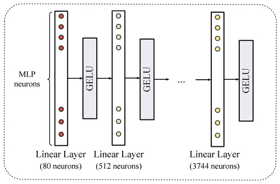
Figure 3. The structure of the MLP Layer. GELU denotes the Gaussian Error Linear Unit.

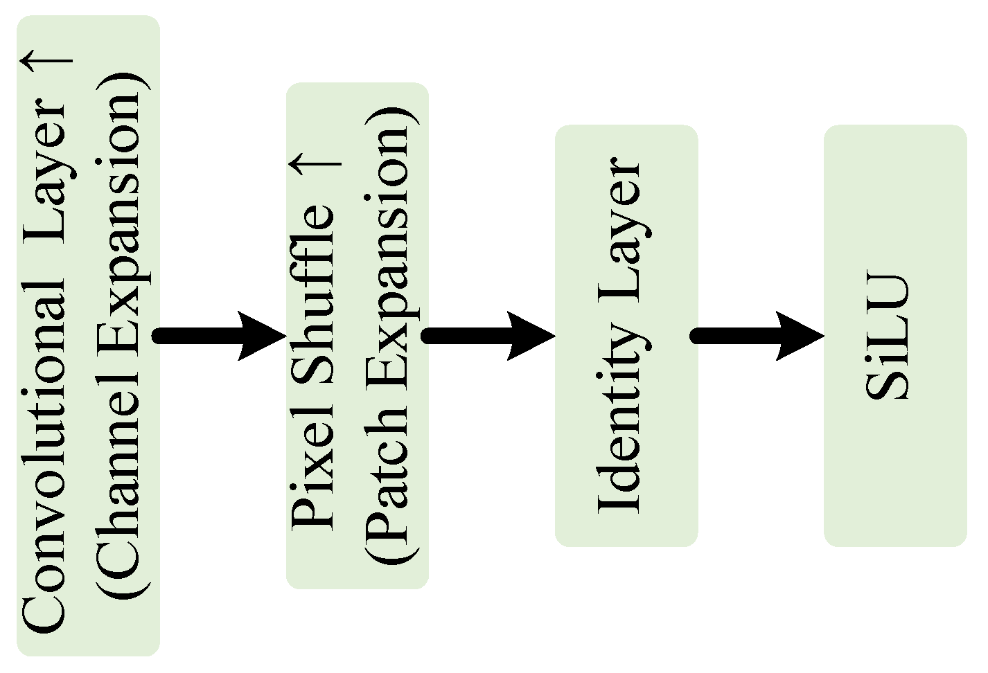
The NeRV block is the essential structure in FIO-F and JSCIFI-F. The network architecture is illustrated in Figure 4.

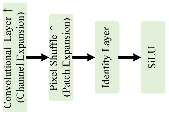
Figure 4. The structure of NeRV block.

Several NeRV blocks express the input video stream as a neural network consisting of multiple convolution operations and output the corresponding three-channel frame information. The PixelShuffle layer [35] is used for upsampling, and higher-quality images can be obtained. Indeed, it is the parameters within all NeRV blocks that store the mapping between positional feature vectors and image features.

For the fusion layer, which takes $E_m$ and $F_2\left(\mathcal{P}\left(t\right)\right)$ as inputs, unlike the spatial–temporal features obtained with pixel multiplication, this feature fusion serves as a distributional shift for $E_{mbedding}$ [16].

$$N_E=Norm\left(\mathrm{TF}\left(\gamma \right)\right)$$

(20)

$$\mu ,\sigma =div\left(F_2\left(\mathcal{P}\left(t\right)\right)\right)$$

(21)

$$F_{fuse\_out}=\left(N_E*\sigma \right)+\mu$$

(22)

where $N_E$ denotes the normalized embedding, and $div\left(\cdot \right)$ is the decomposition operation, which is performed in the channel dimension. $\mu$ and $\sigma$ denote the bias vector and the scale vector, respectively.

JSCIFI-F only uses a simple version of the transformer block where Q, K, and V illustrate the query, key, and value tensor in domain transformation, since the number of parameters determines the compression ratio. Smaller networks also play a role in domain migration, while having a more beneficial effect on hyperspectral image compression.

The architecture of the transformer layer and the attention block are illustrated in Figure 5.

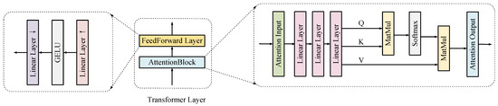
Figure 5. Detailed architecture of the transformer layer.

4. Experiments and Analysis

4.1. Dataset

Chikusei: captured by the Headwall Hyperspec-VNIR-C imaging sensor, these data cover the agricultural and urban areas of Chikusei with a wavelength range of 363–1018 nm and a spatial resolution of 2.5 m. The image size is 2517 × 2335, with 128 spectral bands.

Botswana: these data on the Okavango Delta in Botswana were acquired with the NASA’s EO-1 satellite with a wavelength coverage of 400–2500 nm, a spatial resolution of 30 m, and a spectral resolution of 10 nm. The spatial size is 1476 × 256, with 145 spectral bands.

Pavia: the image sets of the Pavia Centre and the University of Pavia were both acquired with the Reflective Optics System Imaging Spectrometer (ROSIS), the former with a spatial size of 1096 × 715 and 102 spectral bands and the latter with a spatial size of 610 × 340 and 103 spectral bands.

Washington DC: hyperspectral data covering the wavelength range of 400–2400 nm were acquired for the Washington DC Mall area. The spatial size is 1280 × 307, with 191 spectral bands.

Salinas: the Salinas data were acquired by the AVIRIS sensor in the Salinas Valley area in California with a spatial resolution of 3.7 m and an image size of 512 × 217. The raw data contain 224 spectral bands, and 204 bands were retained after removing bands heavily affected by water vapor absorption. The data cover 16 crop classes.

4.2. Evaluation Metrics

We employed bits per pixel per band (bpppb) as a measure of the compression ratio of hyperspectral images (HSIs). In order to fully assess the distortion of the reconstructed images, the following three common quality assessment metrics were used:

(a)

Peak Signal-to-Noise Ratio (PSNR) [36]: it quantifies reconstruction quality by calculating the pixel-level difference between the reconstructed image and the original image; a higher PSNR value indicates higher fidelity of the reconstructed image;

(b)

Multi-scale structural similarity index (MS-SSIM) [37]: it provides a more comprehensive visual quality assessment than the single-scale SSIM by evaluating the luminance, contrast, and structural similarity of an image and combining them with multi-scale analysis;

(c)

Spectral Angle Mapping (SAM) [38]: it assesses reconstruction quality by calculating the angle between the spectral vectors of the original and reconstructed images in spectral space, where a smaller angle indicates better reconstruction.

$$\mathrm{SAM}={\displaystyle \frac{1}{WH}}{\displaystyle \sum }_{w=0}^{W-1}{\displaystyle \sum }_{h=0}^{H-1}{\displaystyle \frac{H_{wh}\cdot {\widehat{H}}_{wh}}{H_{wh}\cdot {\widehat{H}}_{wh}}}$$

(23)

where $H_{wh}\in {ℝ}^{I\times 1}$ denotes the information of the original HSI at position $\left(w,h\right)$, and ${\widehat{H}}_{wh}$ denotes that of the constructed HIS. We employed SAM to further evaluate the construction quality of interspectral similarity.

4.3. Training Setup

The Pytorch framework was employed for network setup. FIO-F and JSCIFI-F were both trained on a server with an NVIDIA 3090 GPU by using the Adam optimizer [39]. To achieve different compression ratios, the network was constructed by using different settings, i.e., by changing the MLP hidden layer, as well as the number and the contained convolutional layer settings of the NeRV blocks. The learning rate was set to 0.0005, and we selected an epoch number of 35.

By referring to a previous method [25,32,34], six hyperspectral datasets were trained, validated, and tested for experiments. To validate the traditional deep learning methods, the mixed dataset was cropped into nonoverlapping 128 × 128 patches and then cut with an overlap in the channel domain (spectral domain) according to the minimum spectral channel number of 48. The split images were divided into three sets in a ratio of 8:1:1. The largest set was used as the training set, while the two smallest sets were used as the validation and test sets, respectively. For the proposed framework, in order to utilize neural video representation, the data in the test set were further divided into frame-like collections. According to the experimental setup, the frame sets were categorized into single-channel and three-channel frame sets.

4.4. Quantitative Results

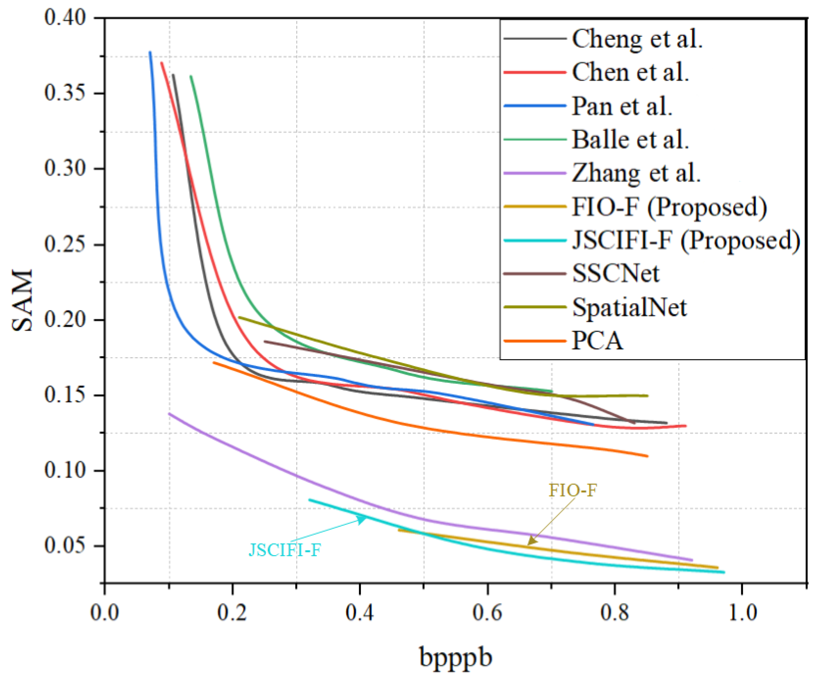
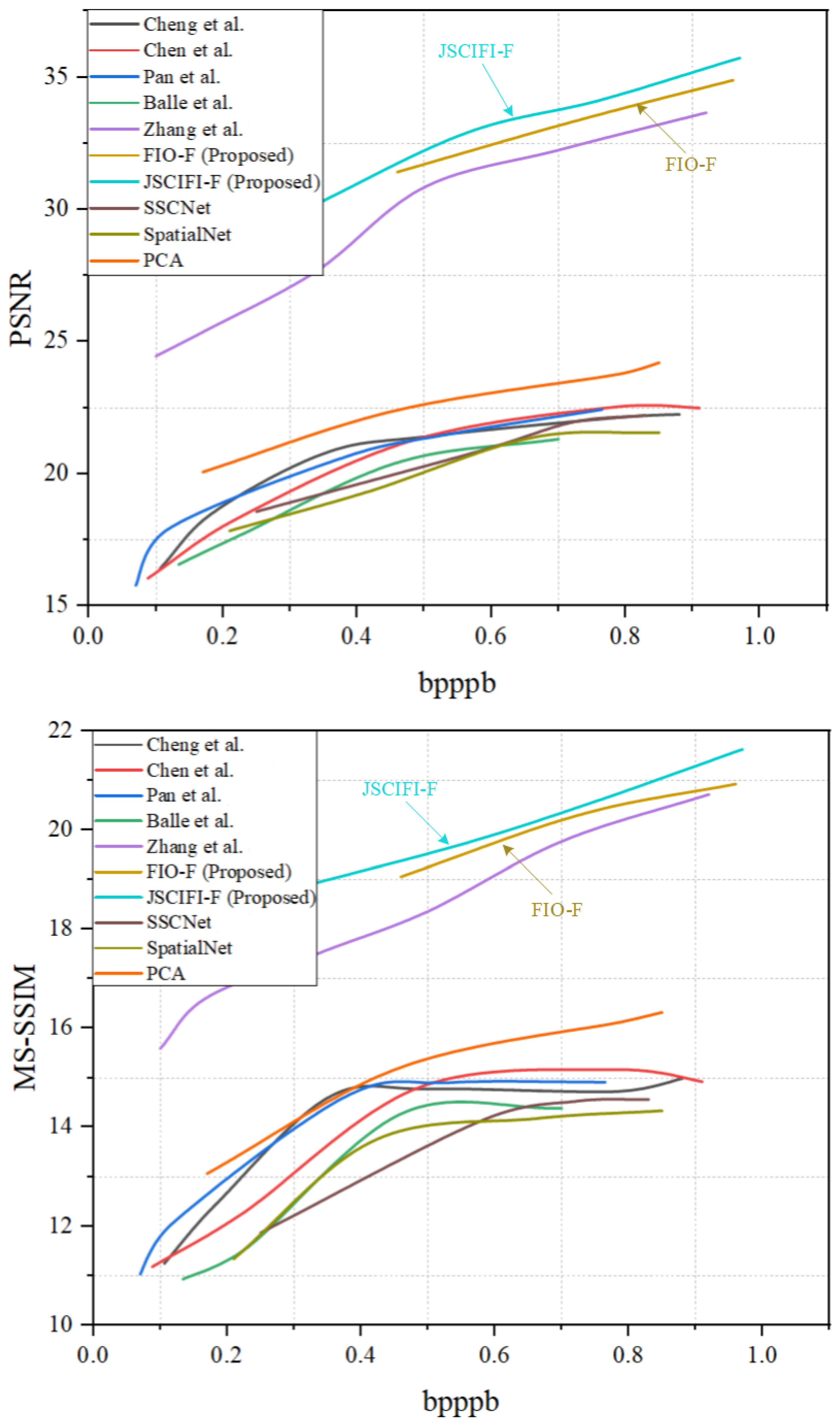
The proposed architectures FIO-F and JSCIFI-F are compared with the methods of Chen et al. [40], Cheng et al. [41], Pan et al. [32], Zhang et al. [34], and Ballé et al. [12], as well as SSCNet [42], SpatialNet [43], and PCA implemented by using sklearn on the generated dataset. Moreover, the results are illustrated in Figure 6 and Figure 7. It can be seen that both FIO-F and JSCIFI-F achieve better results on mixed datasets, far exceeding traditional deep learning methods. In addition, they outperform the fast neural radiation field approach. Compared with traditional deep learning methods, FIO-F, JSCIFI-F, and FHNeRF [34] all achieve nearly 12 dB in PSNR, 15 dB in MS-SSIM, and 0.05 in SAM, demonstrating that neural representations are superior to traditional deep learning methods in RD metrics when hyperspectral datasets do not meet the demands of deep learning feature extraction. Moreover, among the neural representation methods, it can be seen that the method based on video stream representation is superior to the method based on neural radiation fields, i.e., FHNeRF [34]. Specifically, the neural radiation field-based method maps the encoded coordinate information to the spectral information of the input hyperspectral image, whereas the video stream representation-based method slices the image into a representation of video frames and then performs signal fitting based on spatial–temporal information or temporal information. We are surprised to find that the PCA method outperforms traditional deep learning methods, which proves that manual feature extraction is superior to neural networks performing feature extraction automatically without sufficient data support.

Figure 6. The overall results of FIO-F and JSCIFI-F compared to FHNeRF and some traditional deep learning-based methods using SAM [12,32,34,40,41,42,43].

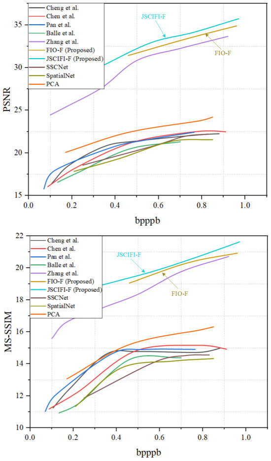
Figure 7. The overall results of FIO-F and JSCIFI-F compared to FHNeRF and some traditional deep learning-based methods using PSNR and MS-SSIM [12,32,34,40,41,42,43].

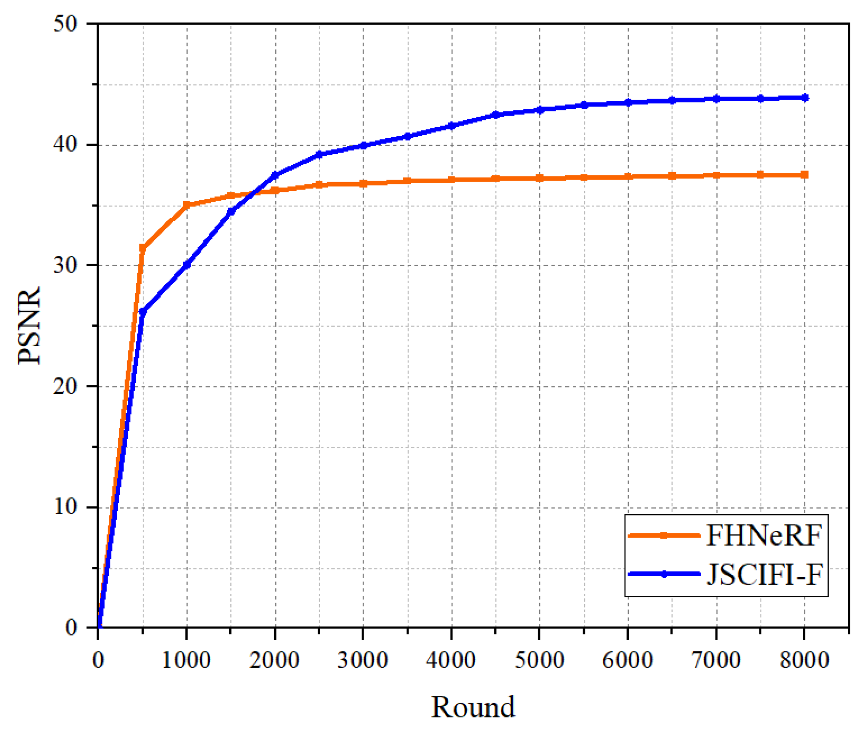
In fact, FHNeRF is designed to meet the need for fast fitting, so the number of training rounds does not achieve optimal compression performance. In order to compare the performance upper bounds of the methods for neural representations more adequately, we take the Botswana dataset as the input to FHNeRF and JSCIFI-F and calculate the number of parameters, the pt-file size, and the fitting speed. The results are illustrated in Figure 8. It can be seen that better results are achieved by JSCIFI-F. FHNeRF training slows down at 5000 rounds of iterations in terms of growth, and the highest PSNR achieved is around 37.5 dB. As for JSCIFI-F, a PSNR of approximately 44 dB is achieved.

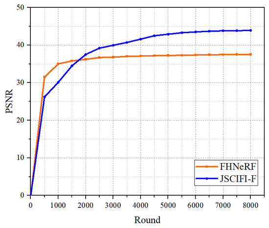
Figure 8. The results on Botswana dataset of FHNeRF (using 0.2 M parameters and achieving a bpppb of 43 compared to the mat file) and JSCIFI-F (using 0.19 M parameters and achieving a compression ratio of 35 compared to the mat file).

We also compare the performance difference between decomposing a hyperspectral image into a three-channel video list and a single-channel video list on the architecture of FIO-F. The results are shown in Table 2.

Table 2. Experimental results of different slicing methods on Botswana dataset using FIO-F.

Dimension Number	PSNR	Training Iterations	Frames
1 dimension	37.62	3000	144
3 dimensions	34.57	3000	48

It can be seen that the performance of the network when a single frame is used as input is not as good as with three-channel frames, and this is easily explained: the single-frame input increases the number of frames, namely it increases the input spatial–temporal dimension, and the network needs to fit more negatively complex data with the same network setup.

Moreover, we compare our model with former deep learning-based methods in neural network complexity. For the output size of the network, given an input index t of a channel, the output is always the size of the patch corresponding to this channel, which, in our experiments, is 256 × 256 or 512 × 512. Then, for the other layers inside the network, changing the number of layers, as well as the size of kernels, can change the number of network parameters, which is the compression ratio. For the proposed method, the size of the network’s parameters represents the compression ratio. We list some of the network settings in Table 3.

Table 3. The network complexity comparison.

Method	Embed	Stem_dim_num	Fc_hw_dim	Strides	Model Size
JSCIFI-F (Ours)	1.25_40	96_1	9_16_26	3_2_2	0.55 M
JSCIFI-F (Ours)	1.25_40	512_1	9_8_13	2_2_2	0.58 M
JSCIFI-F (Ours)	1.25_40	128_1	9_8_13	2_2_2	0.19 M
Cheng et al. (192 channels) [41]	-	-	-	-	18.4 M
Cheng et al. (256 channels) [41]	-	-	-	-	31.7 M
Chen et al. (192 channels) [40]	-	-	-	-	47.7 M
Minnen et al. [44]	-	-	-	-	12 M
Li et al. (192 channels) [45]	-	-	-	-	69.6 M
Li et al. (256 channels) [45]	-	-	-	-	122.7 M
Qian et al. [46]	-	-	-	-	12 M

4.5. Qualitative Results

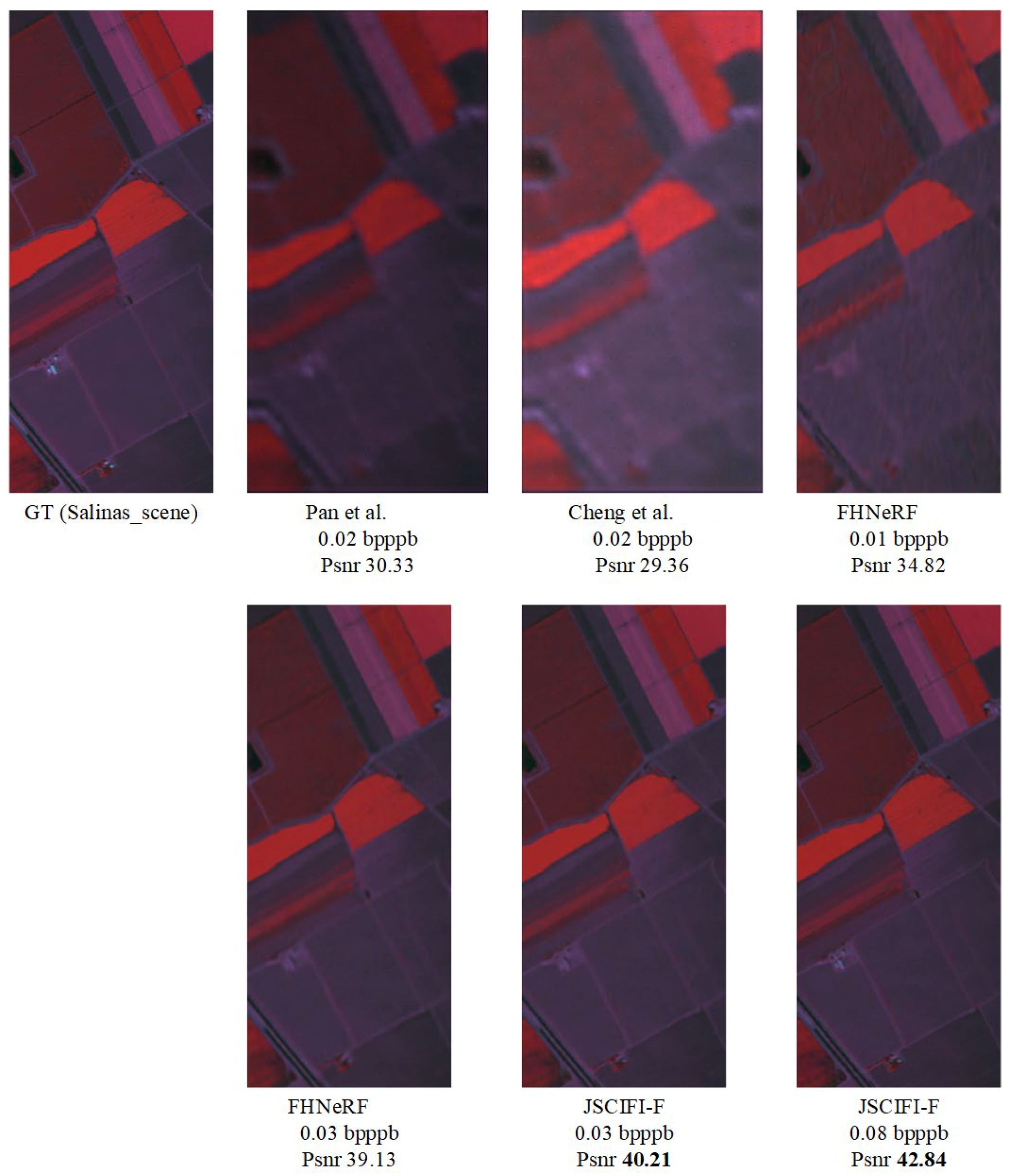
To further evaluate the model’s performance, we conducted experiments by using both traditional deep learning compression methods and the new paradigms (FHNeRF and JSCIFI-F). For a fair comparison, we also overfitted the deep learning methods on the same dataset to obtain results. The results are illustrated in Figure 9 and Figure 10.

Figure 9. Visual results using different methods on Salinas scene dataset [32,34,41].

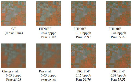
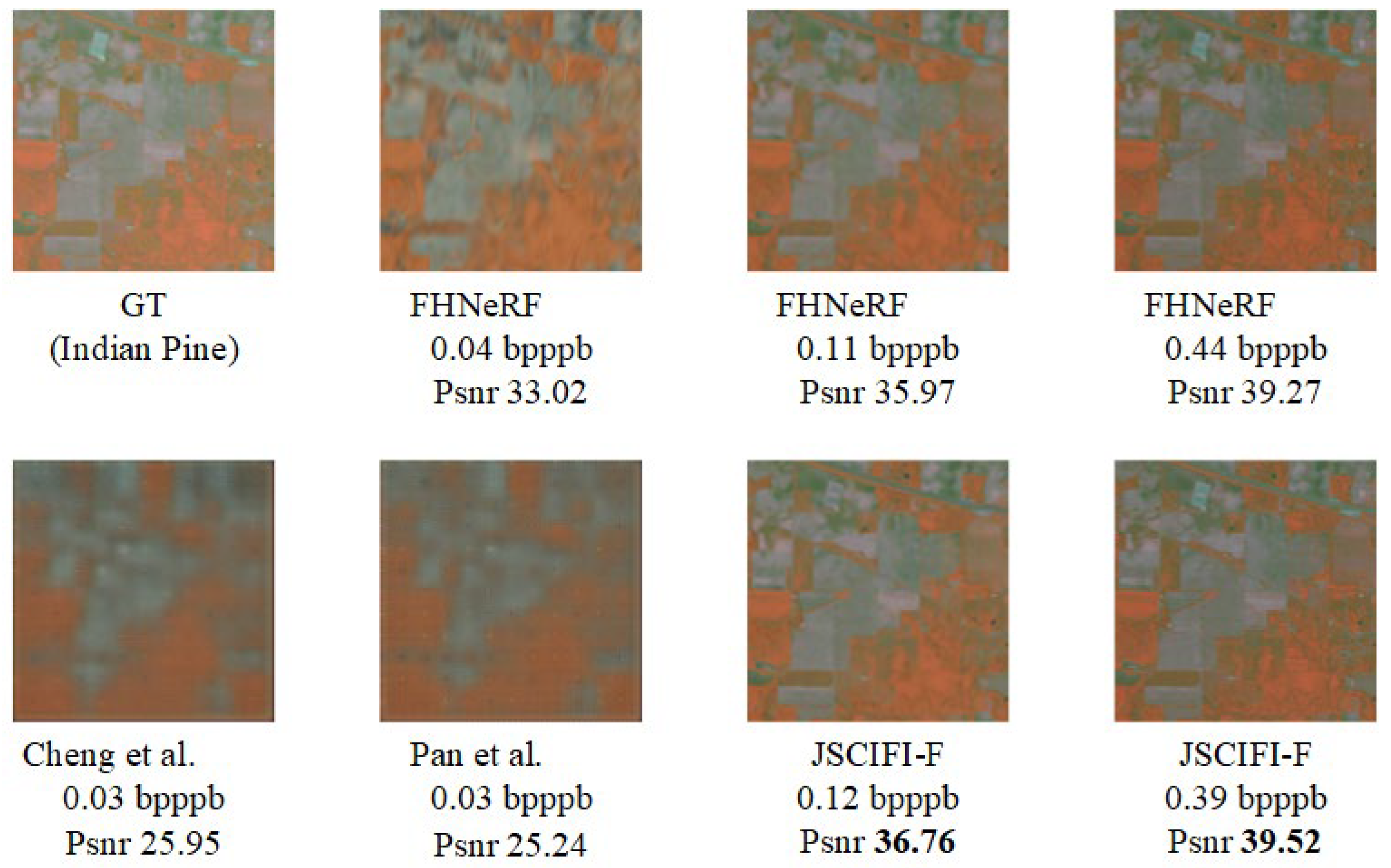
Figure 10. Visual results using different methods on Indian Pine dataset [32,34,41].

It can be observed that even when overfitting is performed on the same dataset, the new paradigms significantly outperform traditional deep learning methods. (In fact, existing deep learning-based feature extraction methods yield much lower results on the current dataset when trained on a training set and tested on a test set compared with being overfitted). Furthermore, different coordinate mapping methods achieve varying results: methods based on video feature representation outperform the FHNeRF method, demonstrating that the input coordinate features have a substantial impact on the model’s fitting ability.

4.6. Downstream Task Evaluation

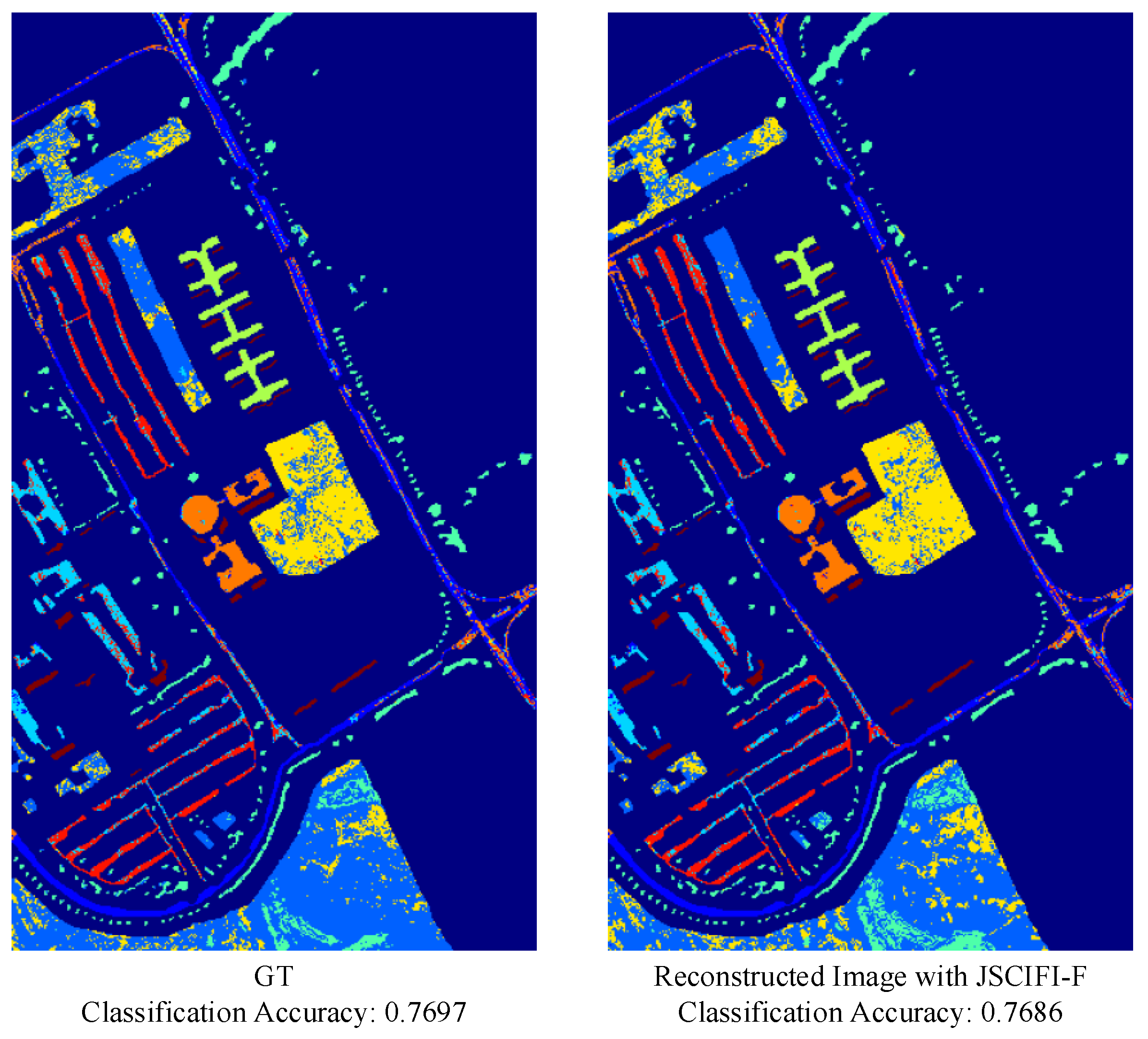
As compressed remote sensing images are typically used for downstream tasks, e.g., classification and object detection, we investigated accuracy in classification tasks by applying the KNN method [47] on compressed images and the JSCIFI-F method on ground-truth images. The results are shown in Figure 11. It can be seen that the proposed compression method does not degrade the performance on the classification task.

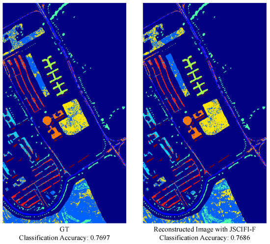
Figure 11. Visual results of HIS classification task.

5. Conclusions

In this study, we develop a new paradigm for compressing hyperspectral images by considering them to be video streams. The paradigm is implemented in two forms, where one consists of generating a coded vector of the temporal dimension (the spectral dimension in the case of hyperspectral images) as input and the other consists of decoupling the temporal and spatial coding and then fusing them to generate images. Both architectures under this paradigm have achieved optimized results, but only using the temporal dimension as input has excessive redundant parameters, resulting in a difficult reduction in the compression ratio, so we prefer the JSCIFI-F architecture. The experimental results demonstrate the superiority of our approach, both in terms of performance metrics and the number of training rounds. We also conclude the drawbacks of the proposed method: perhaps higher computational costs when compressing large volumes of data as well as difficulties in controlling the compression ratio.

References

- Acosta, I.C.C.; Khodadadzadeh, M.; Tusa, L.; Ghamisi, P.; Gloaguen, R. A machine learning framework for drill-core mineral mapping using hyperspectral and high-resolution mineralogical data fusion. IEEE J. Sel. Top. Appl. Earth Obs. Remote Sens. 2019, 12, 4829–4842. [Google Scholar] [CrossRef]
- Stuart, M.B.; Davies, M.; Hobbs, M.J.; Pering, T.D.; McGonigle, A.J.; Willmott, J.R. High-resolution hyperspectral imaging using low-cost components: Application within environmental monitoring scenarios. Sensors 2022, 22, 4652. [Google Scholar] [CrossRef] [PubMed]
- Mahesh, S.; Jayas, D.S.; Paliwal, J.; White, N.D.G. Hyperspectral imaging to classify and monitor quality of agricultural materials. J. Stored Prod. Res. 2015, 61, 17–26. [Google Scholar] [CrossRef]
- Behling, R.; Bochow, M.; Foerster, S.; Roessner, S.; Kaufmann, H. Automated GIS-based derivation of urban ecological indicators using hyperspectral remote sensing and height information. Ecol. Indic. 2015, 48, 218–234. [Google Scholar] [CrossRef]
- Wan, Y.; Hu, X.; Zhong, Y.; Ma, A.; Wei, L.; Zhang, L. Tailings reservoir disaster and environmental monitoring using the UAV-ground hyperspectral joint observation and processing: A case of study in Xinjiang, the belt and road. In Proceedings of the 2019 International Geoscience and Remote Sensing Symposium, IGARSS, Yokohama, Japan, 28 July–2 August 2019. [Google Scholar]
- Hagag, A.; Fan, X.; Abd El-Samie, F.E. HyperCast: Hyperspectral satellite image broadcasting with band ordering optimization. J. Vis. Commun. Image Represent. 2017, 42, 14–27. [Google Scholar] [CrossRef]
- Luo, L.; Chang, Q.; Gao, Y.; Jiang, D.; Li, F. Combining different transformations of ground hyperspectral data with unmanned aerial vehicle (UAV) images for anthocyanin estimation in tree peony leaves. Remote Sens. 2022, 14, 2271. [Google Scholar] [CrossRef]
- Wallace, G.K. The JPEG still picture compression standard. IEEE Trans. Consum. Electron. 1992, 38, xviii–xxxiv. [Google Scholar] [CrossRef]
- Skodras, A.; Christopoulos, C.; Ebrahimi, T. The JPEG 2000 still image compression standard. IEEE Signal Process. Mag. 2001, 18, 36–58. [Google Scholar] [CrossRef]
- Kovalenko, B.; Lukin, V.; Vozel, B. BPG-Based lossy compression of three-channel noisy images with prediction of optimal operation existence and its parameters. Remote Sens. 2023, 15, 1669. [Google Scholar] [CrossRef]
- Fjeldtvedt, J.; Orlandić, M.; Johansen, T.A. An efficient real-time FPGA implementation of the CCSDS-123 compression standard for hyperspectral images. IEEE J. Sel. Top. Appl. Earth Obs. Remote Sens. 2018, 11, 3841–3852. [Google Scholar] [CrossRef]
- Ballé, J.; Minnen, D.; Singh, S.; Hwang, S.J.; Johnston, N. Variational Image Compression with a Scale Hyperprior. arXiv 2018, arXiv:802.01436. [Google Scholar]
- Mildenhall, B.; Srinivasan, P.P.; Tancik, M.; Barron, J.T.; Ramamoorthi, R.; Ng, R. NeRF: Representing Scenes as Neural Radiance Fields for View Synthesis. In Proceedings of the ECCV, Glasgow, UK, 23–28 August 2020. [Google Scholar]
- Ju, J.; Tseng, C.W.; Bailo, O.; Dikov, G.; Ghafoorian, M. DG-Recon: Depth-Guided Neural 3D Scene Reconstruction. In Proceedings of the ICCV, Paris, France, 1–6 October 2023. [Google Scholar]
- Chen, H.; He, B.; Wang, H.; Ren, Y.; Lim, S.N.; Shrivastava, A. Nerv: Neural Representations for Videos. Adv. Neural Inf. Process. Syst. 2021, 34, 21557–21568. [Google Scholar]
- Li, Z.; Wang, M.; Pi, H.; Xu, K.; Mei, J.; Liu, Y. E-Nerv: Expedite Neural Video Representation with Disentangled Spatial-Temporal Context. In Proceedings of the ECCV, Tel Aviv, Israel, 23–27 October 2022. [Google Scholar]
- Lam, E.Y.; Goodman, J.W. A mathematical analysis of the DCT coefficient distributions for images. IEEE Trans. Image Process. 2000, 9, 1661–1666. [Google Scholar] [CrossRef]
- Selesnick, I.W. The double-density dual-tree DWT. IEEE Trans. Signal Process. 2004, 52, 1304–1314. [Google Scholar] [CrossRef]
- He, D.; Yang, Z.; Peng, W.; Ma, R.; Qin, H.; Wang, Y. Elic: Efficient learned image compression with unevenly grouped space-channel contextual adaptive coding. In Proceedings of the CVPR, New Orleans, LA, USA, 18–24 June 2022. [Google Scholar]
- Liu, J.; Heming, S.; Jiro, K. Learned image compression with mixed transformer-cnn architectures. In Proceedings of the CVPR, Vancouver, BC, Canada, 18–22 June 2023. [Google Scholar]
- Fu, H.; Liang, F.; Lin, J.; Li, B.; Akbari, M.; Liang, J.; Han, J. Learned image compression with gaussian-laplacian-logistic mixture model and concatenated residual modules. IEEE Trans. Image Process. 2023, 32, 2063–2076. [Google Scholar] [CrossRef] [PubMed]
- Xiang, S.; Liang, Q. Remote sensing image compression based on high-frequency and low-frequency components. IEEE Trans. Geosci. Remote Sens. 2024, 62, 5604715. [Google Scholar] [CrossRef]
- Zhang, Z.; Qiu, H.; Zhang, M.; Liu, J.; Chen, B.; Zhang, T.; Li, H. COSMIC: Compress Satellite Images Efficiently via Diffusion Compensation. In Proceedings of the NeurIPS, Vancouver, BC, Canada, 10–15 December 2024. [Google Scholar]
- Mijares i Verdú, S.; Ballé, J.; Laparra, V.; Bartrina-Rapesta, J.; Hernández-Cabronero, M.; Serra-Sagristà, J. A Scalable Reduced-Complexity Compression of Hyperspectral Remote Sensing Images Using Deep Learning. Remote Sens. 2023, 15, 4422. [Google Scholar] [CrossRef]
- Guo, Y.; Tao, Y.; Chong, Y.; Pan, S.; Liu, M. Edge-guided hyperspectral image compression with interactive dual attention. IEEE Trans. Geosci. Remote Sens. 2022, 61, 5500817. [Google Scholar] [CrossRef]
- Fuchs, M.H.P.; Rasti, B.; Demir, B. HyCoT: A Transformer-Based Autoencoder for Hyperspectral Image Compression. arXiv 2024, arXiv:2408.08700. [Google Scholar]
- Afrin, A.; Al Mamun, M. Efficient Hyperspectral Data Compression using 3D Convolutional Autoencoder. In Proceedings of the ICAEEE, Dhaka, Bangladesh, 25–27 April 2024. [Google Scholar]
- Shalev-Shwartz, S.; Ben-David, S. Understanding Machine Learning: From Theory to Algorithms; Cambridge University Press: Cambridge, UK, 2014. [Google Scholar]
- Bartlett, P.L.; Mendelson, S. Rademacher and Gaussian complexities: Risk bounds and structural results. J. Mach. Learn. Res. 2002, 3, 463–482. [Google Scholar]
- Vapnik, V.N. An overview of statistical learning theory. IEEE Trans. Neural Netw. 1999, 10, 988–999. [Google Scholar] [CrossRef]
- Haussler, D. Decision theoretic generalizations of the PAC model for neural net and other learning applications. Inf. Comput. 1992, 100, 78–150. [Google Scholar] [CrossRef]
- Pan, T.; Zhang, L.; Qu, L.; Liu, Y. A Coupled Compression Generation Network for Remote-Sensing Images at Extremely Low Bitrates. IEEE Trans. Geosci. Remote Sens. 2023, 61, 5608514. [Google Scholar] [CrossRef]
- Tancik, M.; Srinivasan, P.; Mildenhall, B.; Fridovich-Keil, S.; Raghavan, N.; Singhal, U.; Ramamoorthi, R.; Barron, J.; Ng, R. Fourier Features Let Networks Learn High-Frequency Functions in Low Dimensional Domains. Adv. Neural Inf. Process. Syst. 2020, 33, 7537–7547. [Google Scholar]
- Zhang, L.; Pan, T.; Liu, J.; Han, L. Compressing Hyperspectral Images into Multilayer Perceptrons Using Fast-Time Hyperspectral Neural Radiance Fields. IEEE Geosci. Remote Sens. Lett. 2024, 21, 5503105. [Google Scholar] [CrossRef]
- Yu, C.; Hong, L.; Pan, T.; Li, Y.; Li, T. ESTUGAN: Enhanced Swin Transformer with U-Net Discriminator for Remote Sensing Image Super-Resolution. Electronics 2023, 12, 4235. [Google Scholar] [CrossRef]
- Hore, A.; Ziou, D. Image quality metrics: PSNR vs. SSIM. In Proceedings of the 2010 20th international conference on pattern recognition, Istanbul, Turkey, 23–26 August 2010; pp. 2366–2369. [Google Scholar]
- Bakurov, I.; Buzzelli, M.; Schettini, R.; Castelli, M.; Vanneschi, L. Structural similarity index (SSIM) revisited: A data-driven approach. Expert Syst. Appl. 2022, 189, 116087. [Google Scholar] [CrossRef]
- Zhang, X.; Li, P. Lithological mapping from hyperspectral data by improved use of spectral angle mapper. Int. J. Appl. Earth Obs. Geoinf. 2014, 31, 95–109. [Google Scholar] [CrossRef]
- Zhang, Z. Improved Adam Optimizer for Deep Neural Networks. In Proceedings of the 2018 IEEE/ACM 26th International Symposium on Quality of Service (IWQoS), Banff, AB, Canada, 4–6 June 2018; pp. 1–2. [Google Scholar]
- Chen, T.; Liu, H.; Ma, Z.; Shen, Q.; Cao, X.; Wang, Y. End-to-End Learnt Image Compression via Non-Local Attention Optimization and Improved Context Modeling. IEEE Trans. Image Process. 2021, 30, 3179–3191. [Google Scholar] [CrossRef] [PubMed]
- Cheng, Z.; Sun, H.; Takeuchi, M.; Katto, J. Learned Image Compression with Discretized Gaussian Mixture Likelihoods and Attention Modules. In Proceedings of the IEEE/CVF Conference on Computer Vision and Pattern Recognition, Seattle, WA, USA, 13–19 June 2020. [Google Scholar]
- La Grassa, R.; Re, C.; Cremonese, G.; Gallo, I. Hyperspectral Data Compression Using Fully Convolutional Autoencoder. Remote Sens. 2022, 14, 2472. [Google Scholar] [CrossRef]
- Dua, Y.; Shankar Singh, R.; Parwani, K.; Lunagariya, S.; Kumar, V. Convolution Neural Network Based Lossy Compression of Hyperspectral Images. Signal Process. 2021, 95, 116255. [Google Scholar] [CrossRef]
- Minnen, D.; Ballé, J.; Toderici, G. Joint autoregressive and hierarchical priors for learned image compression. Adv. Neural Inf. Process. Syst. 2018, 31. [Google Scholar]
- Li, H.; Pan, T.; Zhang, L. Enhanced Remote Sensing Image Compression Method Using Large Network with Sparse Extracting Strategy. Electronics 2024, 13, 2677. [Google Scholar] [CrossRef]
- Qian, Y.; Tan, Z.; Sun, X.; Lin, M.; Li, D.; Sun, Z.; Li, H.; Jin, R. Learning accurate entropy model with global reference for image compression. arXiv 2020, arXiv:2010.08321. [Google Scholar]
- Tu, B.; Wang, J.; Kang, X.; Zhang, G.; Ou, X.; Guo, L. KNN-based representation of superpixels for hyperspectral image classification. IEEE J. Sel. Top. Appl. Earth Obs. Remote Sens. 2018, 11, 4032–4047. [Google Scholar] [CrossRef]
Disclaimer/Publisher’s Note: The statements, opinions and data contained in all publications are solely those of the individual author(s) and contributor(s) and not of MDPI and/or the editor(s). MDPI and/or the editor(s) disclaim responsibility for any injury to people or property resulting from any ideas, methods, instructions or products referred to in the content. |
© 2025 by the authors. Licensee MDPI, Basel, Switzerland. This article is an open access article distributed under the terms and conditions of the Creative Commons Attribution (CC BY) license (https://creativecommons.org/licenses/by/4.0/).