Abstract
The accurate detection of individual tree crowns and estimation of tree density is essential for effective forest management, biodiversity assessment, and ecological monitoring. The precision of tree crown detection algorithms plays a critical role in providing reliable data for these applications, where even slight inaccuracies can lead to significant deviations in tree population estimates and ecological indicators. Various algorithmic parameters, such as pixel size and crown segmentation thresholds, can substantially impact tree crown detection accuracy. This study aims to explore the influence of tree stand features and parameters on the effectiveness of the individual tree crown detection method based on a watershed algorithm, leading to identifying optimal configurations that enhance the reliability of forest inventories and support sustainable management practices. Our analysis of the algorithm results shows that the features of the tree stand, such as tree height variance and tree crown size variance, significantly impact the algorithm’s output in precisely estimating tree count. Consequently, adjusting the pixel size of a canopy height model in the context of tree stand features is necessary to minimize error. Additionally, our findings show that there is a need to carefully assess the criterion of membership of a detected tree crown in a circular sample plot, which we based on the point cloud.
1. Introduction
Precision forestry [1,2,3,4] is an innovative approach that utilizes advanced technologies and data analytics to enhance forest management practices with exceptional accuracy and efficiency. By incorporating tools like remote sensing, geographic information systems (GIS), and machine learning, precision forestry enables detailed analyses of forest resources, including tree health, growth patterns, species diversity, and biomass. This data-driven method promotes sustainable forestry by empowering managers to make informed decisions that balance productivity with ecological preservation [5].
A thorough and accurate forest description is crucial for understanding the structure and dynamics of forest ecosystems, enabling well-informed conservation and management strategies [6]. Key metrics—such as tree density, spatial distribution, species composition, and health status—allow for comprehensive biodiversity assessments and continuous monitoring of forest changes, including the impacts of climate change and human intervention. High-quality data on forest conditions also support sustainable resource management by helping predict future trends and mitigate the adverse effects of environmental degradation. With the support of modern technology, precision forestry has become a fundamental tool for advancing sustainable forestry practices [7].
Individual tree crown detection and delineation (ITCD) methods based on a canopy height model (CHM) are designed and widely used to identify and analyze tree crowns within forested areas to improve tree stand metrics precision [8]. These methods leverage the detailed vertical information captured in CHM data, typically derived from LiDAR or photogrammetric sources, to distinguish the height and spatial distribution of tree canopies. By isolating individual crowns, researchers and forest managers can obtain the precise metrics of tree stands. One of the ITCD algorithms, based on a watershed algorithm [9], treats a CHM as a topographic surface. The watershed algorithm identifies distinct “basins” or regions corresponding to individual tree crowns. One of the main problems with this kind of algorithm is proper parameterization, as various tree stands differ in the shape and size of tree canopies [10].
Various studies have performed the watershed algorithm alongside other methods and techniques enhancing the quality of the results of ITCD [10,11]. Many researchers have used marker-controlled watershed [12], which first focuses on finding treetops with local maxima filter [13]. Other researchers [14] have built upon the watershed algorithm by adding clustering techniques, such as spectral clustering or center evolution clustering [15]. The watershed algorithm, with proper preprocessing and postprocessing, becomes a very powerful tool for ITCD. Many studies have investigated how the tree stand characteristics influence the errors of ITCD techniques [16,17].
Many studies have shown the effectiveness of CHM-based methods [18], but many need help to identify conditions for choosing the best parameterization of the algorithm. As many conditions influence the parameters of a tree stand, they should be taken into account before performing CHM-based methods identifying individual tree crowns. When there are vast instances of results on ITCD methods, it takes effort to deal with the dimensionality of the data, and an analysis of the experiment’s results becomes problematic [10]. To mitigate this problem, we can describe probabilistic relationships among tree stand features, algorithm parameters, and results error. Such relationships can be further analyzed in the context of obtained error.
Bayesian networks (BNs) [19,20] are probabilistic models that represent relationships between different variables in the form of a directed graph, where each node stands for a variable, and the connections between those variables reflect probabilistic dependencies. BNs allow us to model and visualize how changes in one variable can affect others, helping us understand complex, uncertain systems. In analyzing data from regression algorithms, such as estimating the number of trees in selected regions, Bayesian networks can be used to examine and interpret the relationships between input features and the predicted outputs. They allow us to assess the influence of each feature on the outcome and detect any patterns or dependencies that might be affecting model performance. This insight helps to refine regression models by identifying essential predictors, understanding uncertainties, and improving overall predictive accuracy by making informed adjustments.
In this study, we analyze the results of the ITCD method based on the watershed algorithm applied to a CHM obtained from airborne laser scanning (ALS) data. The choice of this algorithm is guided by its popularity. We focus our analysis on the features of tree stands and algorithm parameters in the context of a tree count estimation based on circular sample plots inventory data. We utilize BNs to describe probabilistic relationships among variables and to analyze how they affect the estimation error. Our results point to the importance of proper local parameterization of the algorithm as well as the proper establishment of the sample plots used for parameter optimization.
2. Materials and Methods
2.1. ALS Materials and Field Data Inventory
2.1.1. Study Area and Sample Plots Data Inventory
As of 2019, 29.6% of Poland’s land area was covered by forests, with over 75% of these forests managed by State Forests (SF), and the majority composed of coniferous stands [19]. Within northeastern Poland lies the vast Knyszyn Forest, an ecologically rich lowland landscape that includes economic forests, protected areas, nature reserves, and Natura 2000 sites, where management activities are limited to allow natural processes to dominate. Our study, focused on the Zajma forest district, located in the Zednia Forest Inspectorate and overseen by the SF Regional Directorate in Białystok, covers 51 km2 of the Knyszyn Forest, constituting more than half of the district’s territory. In 2016, this area experienced substantial hurricane-induced damage, creating a unique opportunity to study the effects of natural disturbances on forest structure. Further supporting this location’s research value, the Zajma forest district was selected for the two-phase research projects Zajma I and II [21,22], which established 140 circular sample plots (SPs) across the Zednia Forest Inspectorate. Moreover, data from this project were used in one of our previous studies concerning individual tree crown detection methods along with another one from the neighboring forest district [10].
In this study, we utilized data from dendrometric measurements collected from ground-based circular sample plots as part of a two-stage research project conducted by the Forest Management and Geodesy Bureau in cooperation with the State Forests, initiated in 2007 and continued in 2017. A key objective of this project was to evaluate the potential of remote sensing data, both passive and active, for determining specific tree and stand parameters, such as top height and stand density. In the project’s first phase, 52 SPs with radii between 20 and 25 m were established. After a decade, dendrometric measurements were repeated on 38 of these plots, as 14 plots were no longer usable due to forest management treatments and the impact of a hurricane in 2016 that affected stands within the study area. Additionally, 102 new SPs were created with radii from 5.64 to 12.62 m, adjusted according to tree stand age classes. The center of each SP was located using a static-mode geodetic-class GNSS (Trimble SPS 882) with a mean positional error of 0.41 m. The measurements for the Zajma I and Zajma II experiments were performed from January to March 2018. Each SP was characterized by location, tree count (with a diameter at breast height (DBH) above 70 mm), and additional plot features. For each tree, detailed dendrometric attributes were recorded, including its location (measured in polar coordinates relative to the SP center), species, DBH (in mm), height (in meters), crown visibility for remote sensing purposes (1—fully visible, 2—partially visible, 3—not visible) [23], and additional characteristics (such as shared crown or significant trunk deflection).
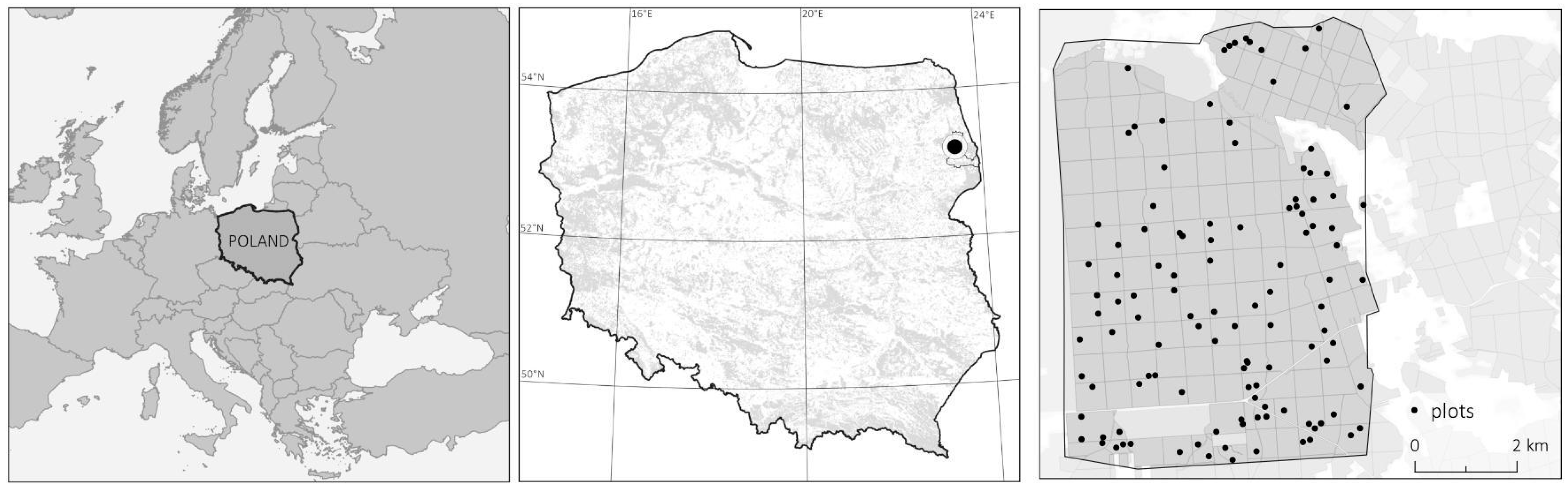
We analyzed results of the individual tree crown detection method based on the watershed algorithm [10] using 112 SPs located in the Zednia Forest District which were dominated by coniferous tree species. Their location, along with the study location area, is presented in Figure 1.
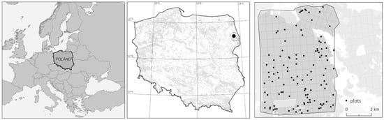
Figure 1.
The study area is located in Northeaster Poland—Central Europe. The middle map shows the location of the Zednia Forest District in Poland with distribution of forested areas in gray. The map on the right presents the distribution of circular ground sample plots in the Zednia Forest District that we used in our study.
The sample plots analyzed in this paper, although situated within the homogeneous area of the Zednia Forest District, can be categorized based on specific local conditions. Accordingly, we have grouped the circular plots according to five primary factors: radius size of the circular plot (A), proportion of gaps in the circular plot (B), variance of the area of the rectangular projection of the crown in the circular plot (C), variance of the height of the trees in the sample plot (D), and proportion of the number of trees with apex partial visibility to complete visibility (E). The ranges of variation for the plot differentiation factors used in our analysis, along with the sample sizes within each class, are presented in Table 1.

Table 1.
The ranges of feature variability grouping the circular sample plots (with counts for each category provided in brackets): radius size of the circular plot (A), proportion of gaps in the circular pot (B), variance of the area of the rectangular projection of the crown in the circular plot (C), variance of the height of the trees in the sample plot (D), and proportion of the number of trees with apex partial visibility to full visibility (E).
The radius size of the circular plot may influence the evaluation process, as with a smaller circular plot, we deal with a higher percentage of trees being on the edge of the circular plot. While dealing with various sample plot sizes, we may need to adjust the inclusion of a tree in a sample plot criterion. In the areas with a high proportion of gaps in the circular plot, the watershed algorithm may be more restricted from creating oversized crowns, which may lead to more trees being detected correctly. The high variance in tree height may result in omitting smaller trees located next to taller trees as smaller trees may be merged into larger trees. A similar situation may occur with a high variance in the area of the rectangular projection of the crown. The trees with a worse visibility class are more challenging to detect and may be omitted by the algorithm by merging into another crown.
2.1.2. Airborne Laser Scanning Point Clouds
As described in our previous study, ALS acquisition flights in the study area were carried out using a Vulcanair P-68 “Observer 2” light aircraft equipped with a Riegl LiteMapper LMSQ-680i laser scanning system. Data processing was completed in RiProcess software, and the resulting point cloud was stored in LAS format version 1.4. Alignment of the XYZ coordinates resulted in the calculated average vertical accuracy not exceeding 0.15 m with horizontal accuracy not exceeding 0.20 m. The point cloud was then classified using TerraScan from the Terrasolid suite. Each point was categorized according to ASPRS standards as follows: 1—unclassified, 2—ground, 3—low vegetation, 4—medium vegetation, 5—high vegetation, 6—buildings and engineering structures, and 7—noise [24]. Table 2 presents the technical parameters of the ALS data acquisition.
Table 2.
Technical parameters of the airborne laser scanning datasets used in this study, including date of acquisition, average scanning density (beam density over the scanning surface), average point cloud density, average density of single-return points (density of beams resulting in a single return), average flight altitude (both above ground level (AGL) and mean sea level (MSL)), scanning coverage, number of scan strips, strip length, data coverage area, and scanning angle (field of view (FOV)).
2.2. Individual Tree Crown Detection Algorithm and Parameter Fitting Benchmark
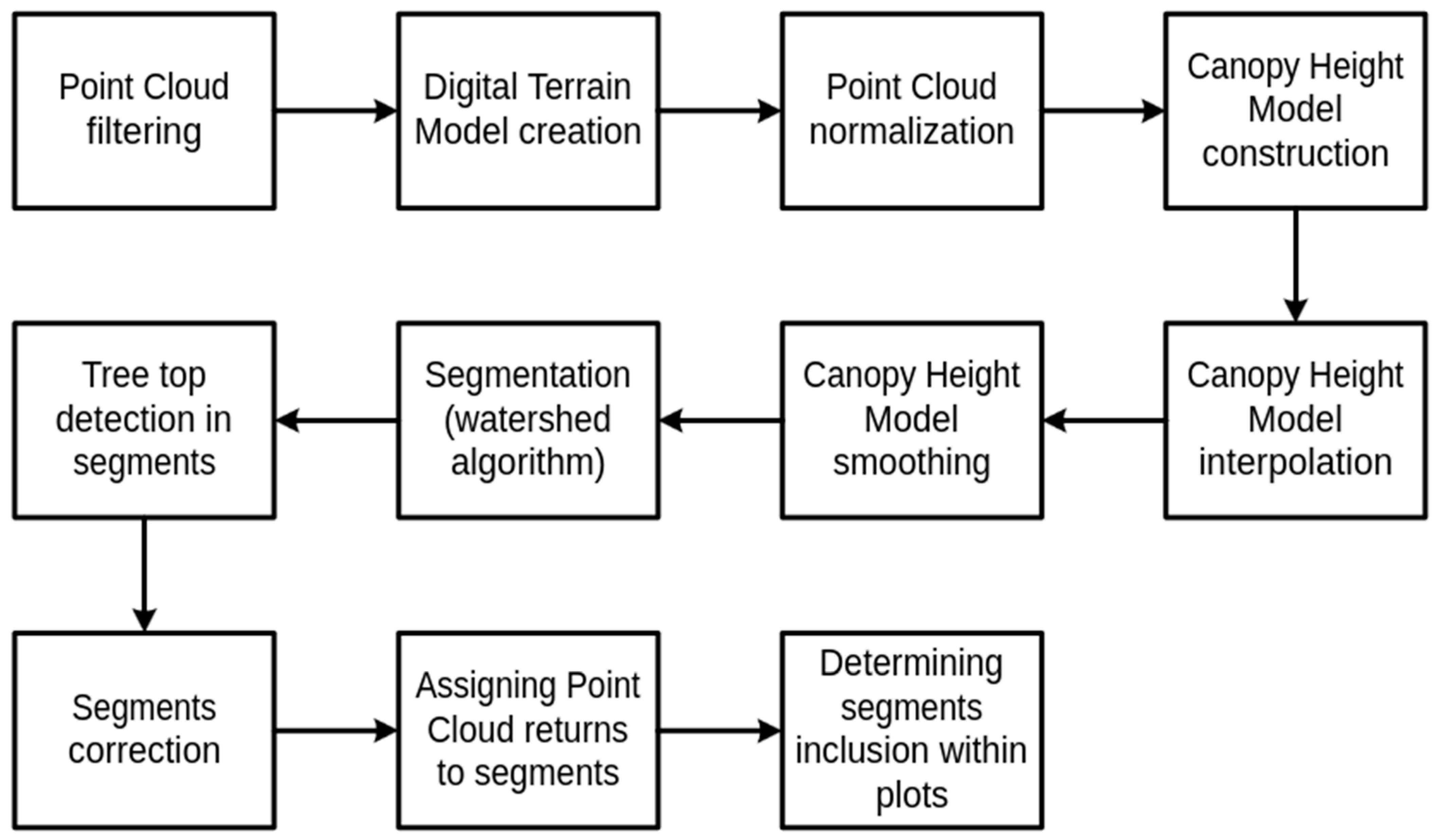
Modern ITCD methods are complex, and multistage algorithms with preprocessing of the data phase and postprocessing of the output of the algorithm to omit easily detectable errors are essential in complex forests stands [25]. The process of adjusting the parameters of the ITCD method requires a proper investigation of its result. Our approach, which has been used in our previous study [10] employing a watershed algorithm, is outlined in Figure 2. The detailed description of each step is as follows:
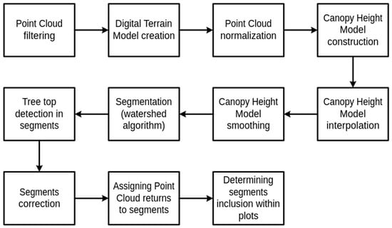
Figure 2.
The general outline of steps in the ITCD method.
- Point Cloud Filtering. The raw point cloud is filtered to remove points of noise class and irrelevant points with a Z coordinate that is too large.
- Digital Terrain Model (DTM) Creation. A DTM raster is generated to represent the bare ground surface by isolating returns of ground class from the point cloud. There are various algorithms to create a DTM, but we used the TIN algorithm, which is a spatial interpolation based on a Delaunay triangulation. This model serves as a reference for tree height calculations and assists in the normalization of the canopy.
- Point Cloud Normalization. The point cloud is normalized by subtracting the DTM height from each point, resulting in a height-above-ground metric. This normalization step transforms the data so that each point’s height represents its distance from the ground, not from sea level, which is essential for accurately measuring tree heights.
- Canopy Height Model (CHM) Construction. The CHM raster is created by using the normalized point cloud to identify the highest points within the canopy at each pixel location. Points lower than 5 m above the ground are omitted due to the irrelevance of small trees and bushes. The size of the pixel is one of the parameters of the described method.
- CHM Raster Interpolation. The CHM is interpolated into a continuous raster format to fill gaps (empty pixels) resulting from insufficient scanning density. We used our proprietary method presented in [10]. It fills missing pixels inside crowns without extending their size. We repeat the procedure of filling the empty pixels that have more than four non-empty pixels as long as no more pixels can be further filled.
- CHM Raster Smoothing. Gaussian smoothing is applied to the CHM raster to reduce noise and small irregularities that could interfere with watershed segmentation. This step simplifies the canopy structure, making it easier to delineate individual tree crowns. We parameterize the smoothing with the smoothing window (mask) size and the standard deviation of the Gaussian distribution used as smoothing mask.
- Segmentation Using the Watershed Algorithm. The watershed algorithm [9] is applied to the smoothed CHM raster to segment individual tree crowns. This algorithm treats the CHM as a topographic surface, dividing the canopy into distinct regions that correspond to individual crowns based on height variations.
- Tree Top Detection in Segments. Within each tree crown segment, treetops are detected by identifying the highest point. Treetop detection is critical for measuring tree height.
- Correction by Merging Trees of a Crown Segment that is Too Small. Detected segments that are too small or represent isolated points are removed or merged with nearby larger tree crown segments. A particular threshold function of height is used to ensure the minimal tree crown size.
- Assigning Point Cloud Returns to Tree Crown Segments. All the relevant points in the point cloud are assigned to their respective tree segments based on spatial alignment with the segmented crowns.
- Determining Segments Inclusion within the analyzed area. For each segment, it is assessed whether the segment belongs to a defined area under consideration based on the assigned points from the point cloud to the tree crown segment. The tree crown is considered to lay in the plot’s area when the percentage of points falling into the SP exceeds the assumed threshold, which can be parameterized.
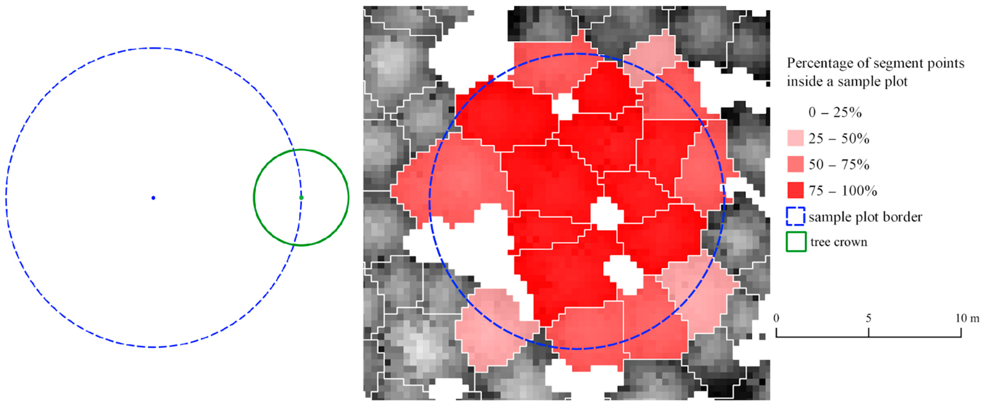
The idea behind steps 10 and 11 is to parameterize the membership of a tree crown segment that emerges from the uncertainty about the location of the segmented tree trunk. To decide whether the tree lies in the circular plot during field dendrometric measurements, the expert measures the distance of the tree’s trunk from the center of the SP. In this case, we do not know the location of the tree trunk. To deal with this problem, we calculate the percentage of returns falling to the SP assigned to the tree segment [10]. Figure 3 presents the problem with a modeled circular tree crown and an example of a circular plot. A tree that has a trunk orthogonal to the ground and located at the edge of the SP has most of its crown outside of the SP. Therefore, we consider different membership thresholds to investigate how they influence the optimization of the ITCD method parameters.
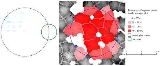
Figure 3.
The modeled circular plot with a tree crown modeled as a circle (the theoretical example) (left) most of the area of the tree crown model falls outside of the sample plot despite the fact that the middle of the tree is located in the sample plot. An example of a real sample plot with tree crown segments with assigned percentage of the segment’s point cloud inside the sample plot expressed as levels of opacity of a red color (right) used to determine the tree membership in the circular sample plot. White areas represent gaps in the canopy height model.
In our experiments, steps 1–6, 10, and 11 were performed using R [26] scripts with the aid of functions available in the lidR library [27]. For steps 7–9, we used the SAGA GIS 8.3.0 free software libraries [28] and QGIS software 3.32.1 [29] geoprocessing models. In step 4, we used the method implemented in the p2r() function [30,31] from the lidR 3.2.3 package to construct a CHM.
2.3. Bayesian Networks
A Bayesian network (BN) [19,20] is a probabilistic model that represents relationships between variables using a directed acyclic graph (DAG). In this graph, nodes represent random variables (such as events or attributes), and directed edges between the nodes indicate conditional dependencies or causal relationships between these variables. The network is grounded in the principles of probability theory and Bayes’ theorem, allowing for the calculation of event probabilities even when there is uncertainty or incomplete information. It is possible because a BN models the joint probability distribution of the variables.
Bayesian networks can be constructed by experts who define the relationships and dependencies between variables based on domain knowledge [32] or by learning directly from the data [33]. When created from data, the process leverages statistical and machine learning techniques to identify the network structure and estimate the conditional probability distributions, which are typically divided into two main steps: structure learning and parameter learning. The latter can be done with simple conditional probability distribution estimation or utilizing techniques like maximum likelihood estimation.
Structure learning techniques fall into two primary categories: score-based algorithms and constraint-based algorithms. Score-based algorithms evaluate different network structures by assigning a score (e.g., Bayesian information criterion) based on how well the structure fits the data. Constraint-based algorithms use statistical tests (like conditional independence tests) to determine the dependencies among variables and then construct the network based on these dependencies.
The PC algorithm [34] (the algorithm’s name comes from the first letters of the authors names) is a constraint-based method for learning the structure of a Bayesian network from data. It identifies conditional independencies among variables and constructs a DAG to represent these dependencies. The algorithm begins with a fully connected graph, where each variable is connected to every other variable. It then iteratively removes edges based on conditional independence tests, determining direct or indirect relationships. Once all edges that represent conditional independencies are removed, the algorithm orients the remaining edges to avoid cycles, resulting in a DAG that captures the underlying causal structure of the variables. The PC algorithm is widely used for structure learning in cases where causal inference is essential, as it provides a clear, interpretable map of dependencies within complex systems. Additionally, an expert may provide background knowledge on some relationships or give temporal information on the variables describing the phenomena appearing in a timeline.
In our study, we used the PC algorithm to build a BN to assess the importance of the ITCD algorithm parameters in the context of various tree stand features. Using the BN model, we can compute the posterior probability of the necessary ITCD algorithm parameter values, which may suggest an optimal setup to optimize the error.
2.4. Strength of Influence Metrics
As we have a BN constructed, we can analyze it in various ways. One of the analyses may focus on analyzing the conditional probability distribution of particular parameters of the ITCD algorithm, given the information on the features of the tree stand. Further, we can investigate the relationships between variables connected with arcs in the BN [35]. To measure the particular dependence, we can use different measures comparing conditional probability distributions defined in the successor nodes given the value of the predecessor node. We focus on three measures in their normalized form available in GeNIe software (Academic Version 5.0.4722.0): Euclidean distance, Hellinger metric, and J-divergence. These measures show us the strength of the interactions between variables [36,37]. When analyzing the strength of influence for each pair of variables connected with a directed arc
We measure distance among all pairs of conditional probability distributions of form
where vi is a possible value of V. When V can have two possible values, than calculation is limited just to one value of distance. In other cases, we need to compute average, weighted average or choose the maximum value among obtained distance values.
In our study, we use these metrics to assess the importance of each parameter of the ITCD algorithm and tree stand features in terms of its strength of influence on error in tree count estimation.
2.4.1. Euclidean Distance
Euclidean distance of two probability distributions
and
takes the following form:
where is the normalizing term. This metric is used due to its simplicity and understandability.
2.4.2. Hellinger Distance
Another measure is Hellinger distance [38], which signifies more values of probabilities closer to 0 and 1. It takes the following form:
2.4.3. Normalized J-Divergence
The Kullback–Leibler distance [39] is widely used for comparing probability distributions. The J-Divergence [40,41] is derived from the Kullback–Leibler divergence and is its symmetrized form. Kullback–Leibler is given by the following formula:
The J-divergence is symmetrized the Kullback–Leibler divergence and has the following form:
Its normalized version has the following form:
The α term is a parameter of the smoothness of the measure and, by default, it is α = 10.
All the algorithms and metrics mentioned above related to BNs are implemented in the GeNIe Modeler (Academic Version 5.0.4722.0, BayesFusion, LLC) which is available free of charge for academic teaching and research use at http://www.bayesfusion.com/ (accessed on 8 November 2024).
2.5. Dataset of the ITCD Results
In our original study [10], we executed the ITCD method based on the watershed algorithm for all sample plots with various parameter sets defining pixel size, standard deviation, and window size of the Gaussian smoothing. In this study, we enhanced the results and calculated the tree count estimates using various thresholds of tree crown membership for the circular sample plot.
Table 3 presents all the variables considered for building BNs. The dataset of results consisted of 84,672 records. The dataset represents the results of the ITCD method in terms of error of tree count estimate calculated for each SP with a varying pixel size (values of {0.35, 0.4, 0.45, 0.5, 0.55, 0.6} in meters are coded as “pix35”, “pix40”, etc.), radius of the window of the Gaussian smoothing mask (values of {1, 2, 3} in pixels resulting in windows 3 × 3, 4 × 4, and 5 × 5 coded as “State1”, “State2”, and “State3”), Gaussian smoothing standard deviation (values in {1, 2, 3} in pixels, coded as “State1”, “State2”, and “State3”) and employing different of tree crown membership thresholds (values from 0.1 to 0.75 with step 0.05 coded as “perc10”, “perc15”, etc.). For the second BN, we took a subset that was concerning the tree crown membership threshold of 0.5. We decided to implement that to compare the resulting structures as the tree crown membership threshold we computed was spread over a long interval, which could lead to a too complicated model and some of the relationships may appear for extreme values of the tree crown membership thresholds. The second model was developed with a dataset of 6048 records.
Table 3.
Variables used to analyze the results.
2.6. Utilizing a BN Model for Parameters Recommendation
Recommendations from the model for parameters of the ITCD algorithm can be obtained by creating a set of observations about tree stand features and determining the degree to which we may want to obtain an error in estimation (in the GeNIe modeler software (Academic Version 5.0.4722.0), it is possible to consider several values of the same variable at the scenario by setting so-called virtual evidence). Then, we calculate the appropriate conditional probability distribution for variables representing the parameters of the ITCD algorithm. Then, iteratively, we also set values with the mode parameter value in the conditional probability distribution of each variable until we set all the ITCD parameters. The obtained set of parameter values can be considered a recommended setup.
3. Results
We first present the resulting BN models and analyze the obtained structures. Then, we analyze the strength of the influence of tree stand features and parameters on the error. Finally, we present an analysis of how the model can be used to analyze the results and to adjust the parameters for various, arbitrary chosen, cases.
3.1. Obtained Bayesian Networks
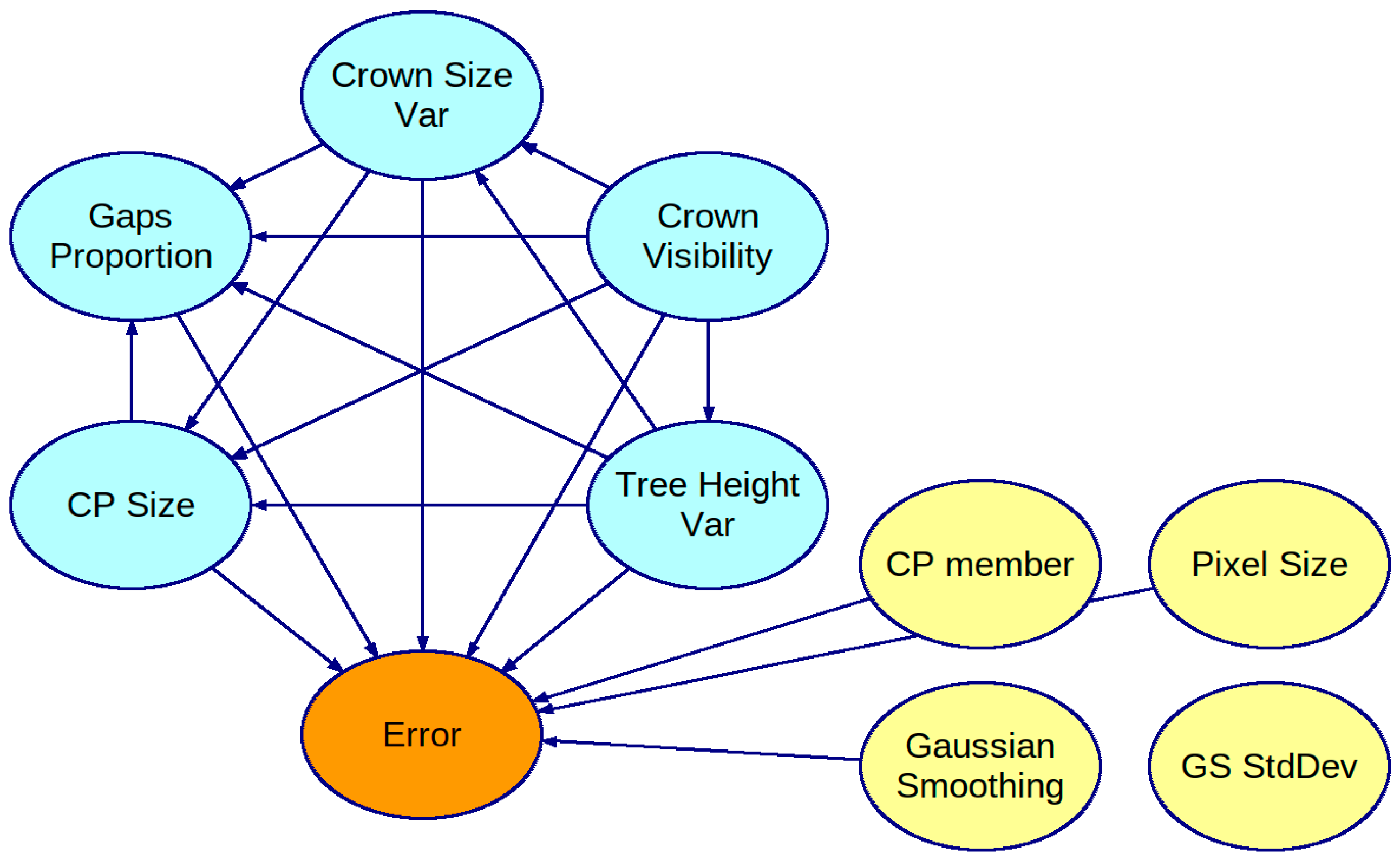
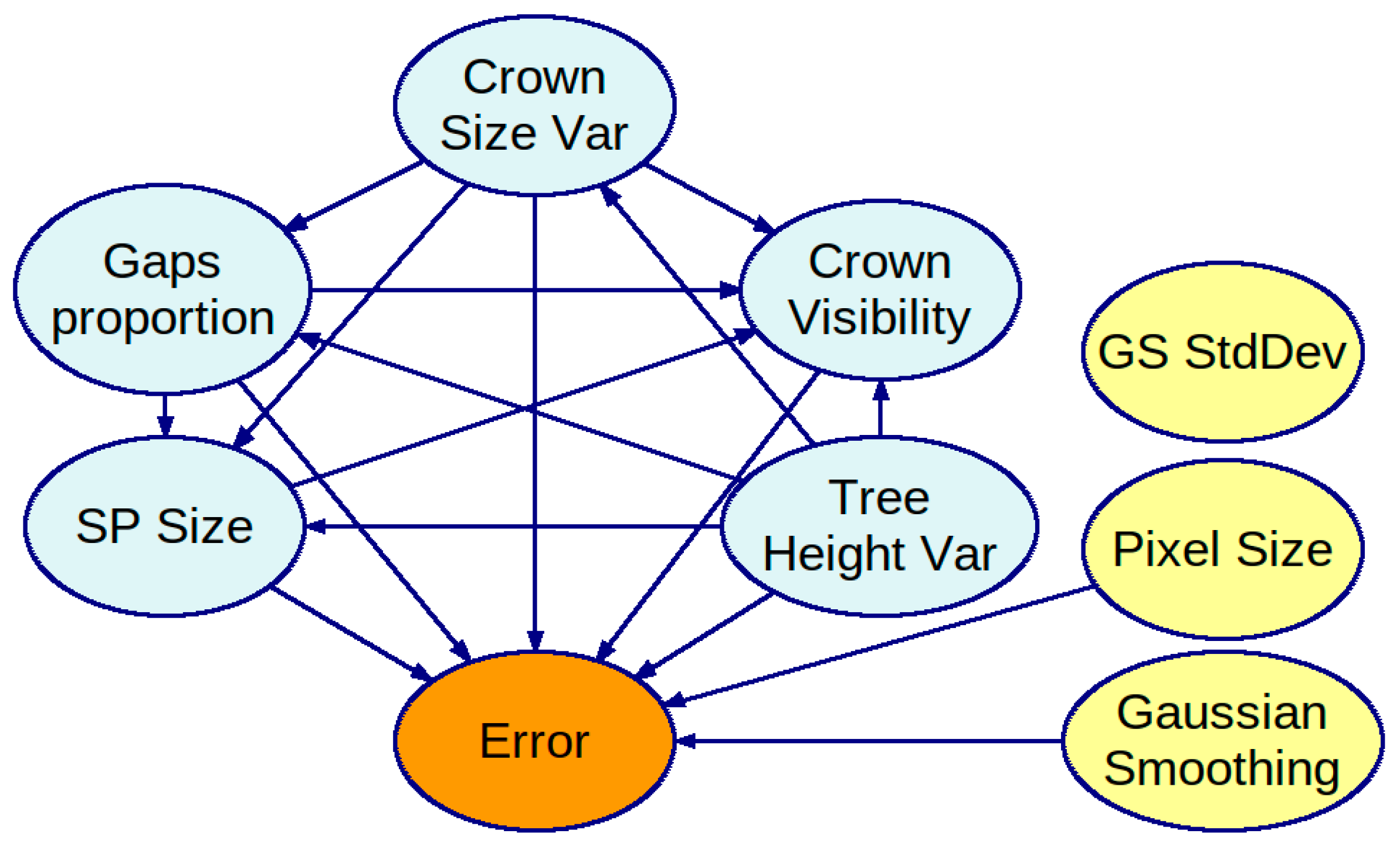
We have built two BNs: one on a complete dataset of results and another on a subset of the dataset, assuming the membership threshold is fixed at 0.5. Figure 4 presents the first BN. All tree stand feature variables are interconnected in the BN’s graph, meaning they depend on each other. The parameters of the ITCD algorithm are assumed to be independent of each other, which complies with common sense, as all of the results were obtained for a grid of the parameters’ values—a Cartesian product of sets of determined values for each ITCD parameter. Thus, there is no statistical dependence among these variables. The PC algorithm rejected the dependence between the standard deviation of the Gaussian Smoothing and other variables in the context of its window size. Consequently, the variable associated with standard deviation (GS StdDev) is isolated without connections to variables in the rest of the graph. Figure 5 shows the second BN. It does not show the variable SP member as its value is equal to 0.5. The variables representing tree stand features are fully interconnected as they are in the first BN, but they are in different directions in some cases. Again, the ITCD method parameters are connected only with the Error variable.

Figure 4.
A Bayesian network created with PC algorithm based on a complete dataset of results for the ITCD method utilizing the watershed algorithm. The tree stand features (in light blue) are interconnected.
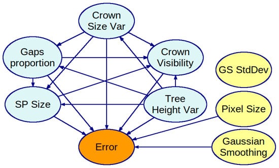
Figure 5.
A Bayesian network created with the PC algorithm using a subset of the dataset of results for the ITCD method utilizing the watershed algorithm, where the sample plot tree membership threshold was 0.5. The tree stand features (in light blue) are interconnected.
In both obtained BN models, the variable representing the standard deviation of the Gaussian kernel used in the smoothing mask is isolated. Therefore, changing it to any of the assumed values does not significantly change the Error distribution.
3.2. Strength of Influence
The strength of influence on the Error variable has been calculated and presented in Table 4, Table 5 and Table 6. We can see that the tree stand features considerably influence the Error more than the ITCD method parameters. The most decisive influence on the algorithm’s error can be found with variables representing the tree height and crown size variance, which are strongly correlated. When comparing different metrics, on average, they show the same ordering of the influencing variables. The most significant difference among metrics can be seen in the maximum value, as it compares extremely different probability distributions. In general, the pixel size of the CHM has the highest value in all metrics among the ITCD parameters.
Table 4.
Euclidean strength of influence on Error in the second Bayesian network.
Table 5.
Hellinger strength of influence on Error in the second Bayesian network.
Table 6.
J-Divergence strength of influence on Error in the second Bayesian network.
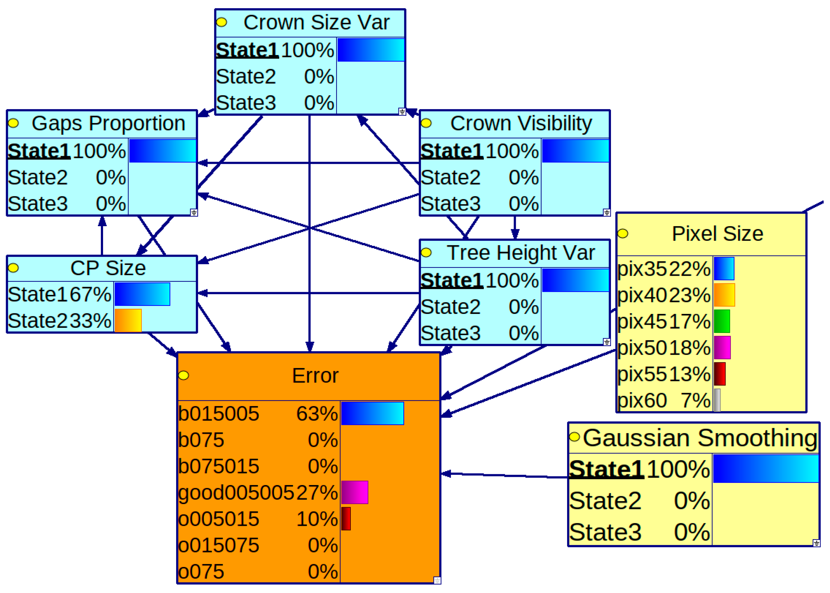
Figure 6 shows the visualization of the calculated average strength of influence for all of the connections in the second BN from the GeNIe modeler software (Academic Version 5.0.4722.0). The thickest arrows inform us about the strongest relationships between variables, which are closely related to a correlation of pairs of variables. For example, Crown Size Var is correlated with Tree Height Var.
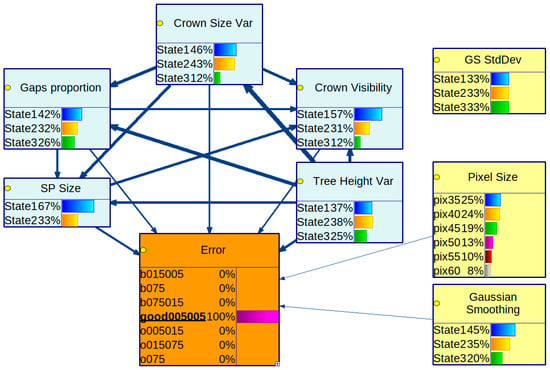
Figure 6.
Visualization of the average strength of influence calculated for all of the connections in the second BN from the GeNIe modeler—the thicker the arrow, the more substantial the influence. Additionally, conditional probability distribution of each variable is calculated given the lowest error, ranging from −0.05 to 0.05, using a membership threshold at a level of 0.5 (assumption of the second Bayesian network). Each conditional probability distribution is presented in the form of a horizontal bar chart. Image prepared with the GeNIe modeler.
3.3. Conditional Probability Distribution
We calculated various conditional probability distributions to investigate the optimal parameters of the ITCD algorithm given the features of circular SPs. For that investigation, we used the first BN, which lets us investigate how the optimal parameters change as we also change the segment membership on the sample plot. Such calculations are straightforward with the software we used to generate the BNs and let us quickly analyze distributions of variables given the set of parameters. For example,
gives a distribution over analyzed pixel sizes of results, assuming we want the smallest Error in tree count estimation and using tree crown membership threshold at level 0.5. The Pixel Size value with the highest probability can be considered optimal in general. The conditional distribution of variable Pixel Size varies under different conditions (e.g., features of a circular SP) when we add them to the condition set, e.g., (SP Size = 1, Error = (−0.05,0.05], CP member = 0.5).
Pr(Pixel Size|Error = (−0.05, 0.05], CP member = 0.5)
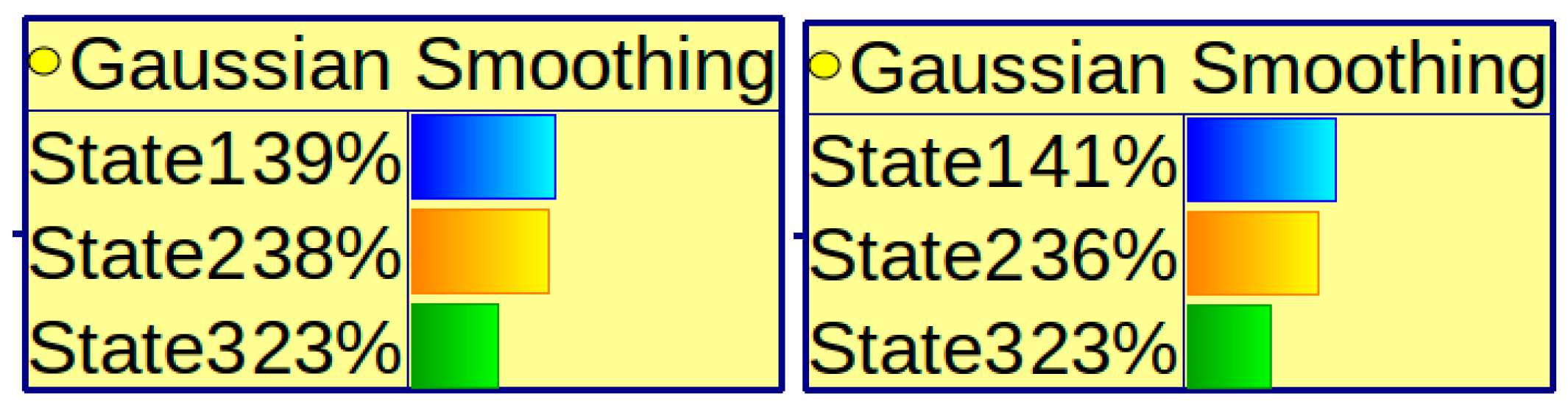
As discussed earlier, we compared two thresholds for the tree crown segment: 0.45 and 0.5. Let us assume that we want to obtain results in an optimal range of Error − (−0.05, 0.05]. Additionally, we are neglecting the sample plot features. Then, for SP member = 0.5, the calculated conditional probability distribution suggests using the smallest smoothing window. When we set Gaussian Smoothing to State1, we can determine the optimal Pixel Size of 0.4 m (probability 0.232).
When we repeat the same calculations for SP member = 0.45, the conditional probability distribution of the Gaussian Smoothing variable slightly changes and suggests the same smoothing window of 1 and pixel size of 0.4 m. In this case, it does not matter whether we adjust parameters under the membership criterion of 0.45 or 0.5.
An investigation of the results depending on the size of the SPs gives slightly different results. When we consider small SPs (SP Size = State1), the recommendation for Gaussian Smoothing is still 1 (Figure 7), but pixel size recommendation changes to 0.4 (probability 0.22) or 0.45 (probability 0.202) when using SP member = 0.5. For SP member = 0.45, the model suggests pixel sizes of 0.4 (probability 0.227) and 0.5 (probability 0.212). For larger SPs (SP Size = State2), the model suggests the same Gaussian Smoothing values, but in both cases a CHM pixel size of 0.35. It means that changes in the criterion of tree membership in the SP influence decisions about the optimal ITCD parameters.

Figure 7.
Differences in conditional probability distributions of Gaussian Smoothing for tree crown membership thresholds equal to 0.45 (left) and 0.5 (right) given the perfect results with tree crown count estimation errors in the range [−0.05, 0.05] for small SPs. Images prepared with the GeNIe modeler.
We can flip the analysis and investigate what the distribution of Error is given suggested parameters. We assume in further analysis that we evaluate the membership of the tree crown in SP with a threshold of 0.45. Table 7 presents conditional probability distributions of Error, when comparing results for Gaussian Smoothing (window size radius) 1 and pixel sizes 0.4 m and 0.45 m across varying SP sizes.
Table 7.
Conditional probability distributions of Error variable (organized in columns), when comparing results for Gaussian Smoothing window size of radius 1 pixel and CHM pixel sizes 0.4 m and 0.45 m across varying SP Size values assuming tree crown membership threshold of 0.45 (State1—smaller SPs, State2—larger SPs).
The distributions show that, in general, the tree count estimation error is closer to 0 when the ITCD algorithm is evaluated on larger SPs. What is important to observe is that the error is spread in the interval (−0.75, 0.75] for Pixel Size = pix40 (0.4 m) and mostly in interval (−0.75, 0.15] for a CHM pixel size of 0.45 m. It is important in situations when regular underestimation is better than overestimation. As the distribution of Error has large variance, we can repeat the investigation for a wider interval (−0.15, 0.15] (the software allows us to choose several possible values for the variable). In such a situation, the model suggested a CHM pixel size of 0.4 m for small SPs and 0.35 m for larger SPs. It proves that the same algorithm setup leads to various error distributions for smaller and larger SPs, and the choice of size of SPs is relevant. Larger SPs have a smaller variance in the error of the tree count estimation.
Further, we analyzed how the features of tree stands influence the change in the conditional distribution of Error and chosen parameters. For good tree Crown Visibility (State1 and State2), the optimal CHM pixel size is 0.4 m. For poor visibility, the most optimal is 0.45 m. Table 8 presents conditional probability tables of Error for the optimal CHM pixel sizes of a given Crown Visibility value. With worse crown visibility in the forest stand, it is hard not to underestimate the tree count, which can be observed in the results.
Table 8.
Examples of conditional probability distributions of error in intervals, when comparing results for Gaussian Smoothing window size 1 and CHM pixel sizes of 0.4 m and 0.45 m according to which CHM pixel size is optimal for tree stand with given crown visibility level (State1—almost all tree crowns have good visibility, State2—some tree crowns have poor visibility, State3—a lot of tree crowns have visibility). The tree crown membership threshold at level of 0.45.
Under the same conditions, when investigating various values of variables representing crown size variance, tree height variance, and proportion of gaps in the CHM, the model suggests using a CHM with a pixel size of 0.4 m. Further we created a scenario for a typical homogenous Scots pine tree stand. We considered the lowest variance in tree crown size and tree height, with the tree crown having a high visibility percentage and a low gap proportion. The scenario applied to the model is shown in Figure 8. We compare how the conditional probability distribution of Pixel Size changes when we adjust the parameters using smaller and larger sample plots. We present these in Table 9. The suggested pixel size is 0.4 m, but in the case of using large SPs for evaluation, we cannot say what would be the best based on the presented model. It is supported by too small a sample size of the subdataset with SPs representing simple tree stands to point to an optimal solution but gives 0.35 m, 0.4 m, and 0.45 m as suggestions.

Figure 8.
A Bayesian network with calculated marginal conditional probability distributions of Pixel Size variable given specific features of the tree stand, and Error is in one of the ranges (−0.15, −0.05], (−0.05, 0.05], or (0.05, 0.15]—suggested use of pixel size of 0.4 m (the dominant probability value).
Table 9.
The conditional probability distribution (organized in columns) of Pixel Size changes when we adjust the parameters using smaller and larger sample plots given specific features of the tree stand and Error is in one of the ranges (−0.15, −0.05], (−0.05, 0.05], or (0.05, 0.15]. The highest probability value is in bold.
4. Discussion
Obtained BNs can provide insight into the results of the ITCD algorithm and its parameterization and help to understand the tree stand features that make the estimation of the tree crown count with the ITCD methods challenging for the algorithm. With various tree stand features, different parameter sets perform better. The size of the CHM pixel, especially, is the most relevant ITCD parameter based on analyzing the strength of the influence of direct interactions of the variables. In the research community, there are studies leading to a decrease in the number of parameters of the ITCD methods to simplify and automate the process of the analysis of forested areas from remote sensing materials [11].
The discrete BNs shown in this paper have some deficiencies in representing the algorithm’s results due to various reasons. We discretized the values of errors into several intervals, as well as other considered variables, which may lead to overgeneralization. The models carry the flaws of the used dataset. We considered only ALS data as the source material for point cloud tree segmentation. This dataset has its own features influencing the correctness of the resulting tree crown segments, e.g., scanning or point cloud density. In practice, the utilization of various source materials, such as UAV laser scanning or photogrammetric point cloud, used for creating a CHM may also influence the results. Further, the choice of tree stands features to differentiate the parameterization of ITCD may need to be expanded to find the optimal global solution, as in this study, we limited the analysis to coniferous forests. On the other hand, when we are too specific about those features, we may require more SP field data to find a significant sample of SPs and adjust the parameters accordingly. Moreover, we used a specific processing pipeline where we used particular methods in each step. In the step of creating a CHM raster, we use the simple method, which is followed by filling the gaps in the CHM raster. Other methods for CHM creation are not covered by this study, which may lead to better results, e.g., the pit-free method [17]. We used our method as it is a good compromise between good results and time efficiency.
The ITCD algorithms can be evaluated from various perspectives. In this study we focused on precise tree count estimation. Many studies register other metrics e.g., omission, commission, or measure proper crown position and delineation. These features could be added in a future analysis.
The size of circular sample plots influences how the algorithm’s accuracy can be evaluated. In this study, we analyzed membership function at several thresholds, focusing on 0.45 and 0.5. In practice, it may be adjusted when dealing with known average tree crown size and sample plot size to mitigate the discrepancy of methods for taking trees into account while conducting field measurements and for counting trees to evaluate the ITCD algorithm.
Various methods have been studied to mitigate the uncertainty problem of the membership of a tree crown to the study area while using circular SPs [42,43,44]. In our study we used the percentage of points falling into the SP as a function of the crown membership. Various conditions and tree stand features may suggest other solutions and it should be investigated in future work.
When planning field surveys and the size of circular SPs for the purpose of adjusting the ITCD parameters to optimize the accuracy of estimating tree crown count, larger sample plots may be considered. However, another problem arises as follows: larger sample plots make the field survey measurements more laborious. So, there is a need for a proper compromise between sample plot size and workload to prepare the data [22]. An alternative is the utilization of virtual sample plots created by an expert based on a set of various remote sensing materials, such as a CHM or orthophoto maps. The expert can establish and outline sample plots along with tree crown segments manually [45,46].
5. Conclusions
Adjusting the parameters of the ITCD algorithms based on a CHM to suit local environmental conditions is crucial for accurate tree crown identification. Localized variations in vegetation, topography, and canopy structure can significantly impact the performance of these algorithms, meaning that parameters must be fine-tuned to deal with specific regional characteristics. This customization improves detection accuracy by accommodating the unique attributes of the forest stand, thereby enabling more reliable results in terms of tree count.
When using circular SPs, matching the ITCD algorithm’s parameters with a suitable membership function that associates each detected tree crown with the circular plot area is essential. This function allows for proper alignment and ensures that each identified crown is accurately attributed to the correct plot. With this alignment, the results may accurately represent tree density and distribution, which can affect subsequent forest structure and biodiversity analyses. In the approach mentioned in this study, the sample plot tree membership has been determined based on the percentage of tree segment returns falling into the sample plot. For circular sample plots, the larger size of sample plots suggests that the choice of sample plot membership percentage threshold should be below but close to 0.5. For smaller sample plots, it can go down to 0.45 as the edge of the circular SP gets rounder.
The post-processing stage of the ITCD results is also a critical step, particularly when filtering out minor, potentially erroneous tree detections, as presented in the previous study [10]. This step allows for refining the detection output by excluding small crowns that may not represent actual tree individuals. Such filtering is especially important in dense or mixed forests, where overlapping canopies and undergrowth could otherwise lead to over-counting or the misidentification of lower vegetation as individual trees. It can use a simple method [10] or try to classify erroneously delineated trees [47].
In the ITCD methods based on the watershed algorithm, which utilizes a CHM, pixel size stands out as the most influential parameter. The choice of pixel size determines the resolution of the crown boundaries and impacts the clarity of the segmentation process. Smaller pixels can capture finer details within the canopy structure, improving the accuracy of crown delineation, while larger pixels may simplify the data but risk losing critical details. Our results suggest the use of a CHM with a pixel size of 0.4 m as a generic solution but, in specific situations, the optimal value shifted to 0.35 m or 0.45 m. Therefore, selecting the optimal pixel size is essential to balance data precision with computational efficiency, ensuring that tree crowns are detected accurately and appropriately within the analyzed forest area. Such adjustment should be taken into account in the context of tree stand features, such as the variance of tree height, as they have the strongest influence on the tree count estimation result. In extreme cases, other ITCD methods should be considered.
Author Contributions
Conceptualization, M.K. (Marcin Kozniewski) and Ł.K.; methodology, M.K. (Marcin Kozniewski); formal analysis, M.K. (Marcin Kozniewski); resources, M.K. (Marek Ksepko); data curation, Ł.K., S.C., M.K. (Marek Ksepko), and M.K. (Marcin Kozniewski); writing—original draft preparation, M.K. (Marcin Kozniewski); writing—review and editing, M.K. (Marcin Kozniewski), S.C. and Ł.K.; visualization, S.C. and M.K. (Marcin Kozniewski); supervision, M.K. (Marek Ksepko); funding acquisition, M.K. (Marek Ksepko). All authors have read and agreed to the published version of the manuscript.
Funding
This study was partially by Bialystok University of Technology under the Grants WZ/WI-IIT/4/2023 and WZ/WB-INL/3/2021 founded by Ministry of Science and Higher Education, Poland. APC was funded by Forest Management and Geodesy Bureau.
Data Availability Statement
Data are contained within the article.
Conflicts of Interest
The authors declare no conflicts of interest.
References
- Panagiotidis, D.; Abdollahnejad, A.; Slavík, M. Assessment of Stem Volume on Plots Using Terrestrial Laser Scanner: A Precision Forestry Application. Sensors 2021, 21, 301. [Google Scholar] [CrossRef] [PubMed]
- Moskal, L.M.; Erdody, T.; Kato, A.; Richardson, J.; Zheng, G.; Briggs, D. Lidar applications in precision forestry. In Proceedings of the Silvilaser 2009, College Station, TX, USA, 14–16 October 2009; pp. 154–163. [Google Scholar]
- Kovácsová, P.; Antalová, M. Precision forestry–definition and technologies. Šumarski List 2010, 134, 603–610. [Google Scholar]
- Dyck, B. Precision forestry—The path to increased profitability. In Proceedings of the Second International Precision Forestry Symposium, University of Washington, Seattle, WA, USA, 15–17 June 2003; Volume 2003, pp. 3–8. [Google Scholar]
- Fardusi, M.J.; Chianucci, F.; Barbati, A. Concept to practice of geospatial-information tools to assist forest management and planning under precision forestry framework: A review. Ann. Silvic. Res. 2017, 41, 3–14. [Google Scholar]
- Instytut Badawczy Leśnictwa (Forest Research Institute). Comprehensive Monitoring of Stand Dynamics in Białowieza Forest Supported with Remote Sensing Techniques (ForBioSensing). 2014. Available online: http://www.forbiosensing.pl/about-project (accessed on 1 November 2024).
- Goodbody, T.R.; Coops, N.C.; Marshall, P.L.; Tompalski, P.; Crawford, P. Unmanned aerial systems for precision forest inventorypurposes: A review and case study. For. Chron. 2017, 93, 71–81. [Google Scholar] [CrossRef]
- Koch, B.; Kattenborn, T.; Straub, C.; Vauhkonen, J. Segmentation of Forest to Tree Objects BT—Forestry Applications of Airborne Laser Scanning: Concepts and Case Studies. In Forestry Applications of Airborne Laser Scanning. Managing Forest Ecosystems; Maltamo, M., Næsset, E., Vauhkonen, J., Eds.; Springer: Dordrecht, The Netherlands, 2013; pp. 89–112. ISBN 978-94-017-8663-8. [Google Scholar]
- Hyyppä, J.; Kelle, O.; Lehikoinen, M.; Inkinen, M. A segmentation-based method to retrieve stem volume estimates from 3-D tree height models produced by laser scanners. IEEE Trans. Geosci. Remote Sens. 2001, 39, 969–975. [Google Scholar] [CrossRef]
- Kolendo, Ł.; Kozniewski, M.; Ksepko, M.; Chmur, S.; Neroj, B. Parameterization of the Individual Tree Detection Method Using Large Dataset from Ground Sample Plots and Airborne Laser Scanning for Stands Inventory in Coniferous Forest. Remote Sens. 2021, 13, 2753. [Google Scholar] [CrossRef]
- Xu, X.; Iuricich, F.; De Floriani, L. A topology-based approach to individual tree segmentation from airborne LiDAR data. GeoInformatica 2023, 27, 759–788. [Google Scholar] [CrossRef]
- Yu, K.; Hao, Z.; Post, C.J.; Mikhailova, E.A.; Lin, L.; Zhao, G.; Tian, S.; Liu, J. Comparison of Classical Methods and Mask R-CNN for Automatic Tree Detection and Mapping Using UAV Imagery. Remote Sens. 2022, 14, 295. [Google Scholar] [CrossRef]
- Popescu, S.C.; Wynne, R.H. Seeing the Trees in the Forest: Using Lidar and Multispectral Data Fusion with Local Filtering and Variable Window Size for Estimating Tree Height. Photogramm. Eng. Remote Sens. 2004, 70, 589–604. [Google Scholar] [CrossRef]
- Liu, Y.; Chen, D.; Fu, S.; Mathiopoulos, P.T.; Sui, M.; Na, J.; Peethambaran, J. Segmentation of Individual Tree Points by Combining Marker-Controlled Watershed Segmentation and Spectral Clustering Optimization. Remote Sens. 2024, 16, 610. [Google Scholar] [CrossRef]
- Li, Y.; Xie, D.; Wang, Y.; Jin, S.; Zhou, K.; Zhang, Z.; Li, W.; Zhang, W.; Mu, X.; Yan, G. Individual tree segmentation of airborne and UAV LiDAR point clouds based on the watershed and optimized connection center evolution clustering. Ecol. Evol. 2023, 13, e10297. [Google Scholar] [CrossRef] [PubMed]
- Ma, K.; Chen, Z.; Fu, L.; Tian, W.; Jiang, F.; Yi, J.; Du, Z.; Sun, H. Performance and Sensitivity of Individual Tree Segmentation Methods for UAV-LiDAR in Multiple Forest Types. Remote Sens. 2022, 14, 298. [Google Scholar] [CrossRef]
- Yang, Q.; Su, Y.; Jin, S.; Kelly, M.; Hu, T.; Ma, Q.; Li, Y.; Song, S.; Zhang, J.; Xu, G.; et al. The Influence of Vegetation Characteristics on Individual Tree Segmentation Methods with Airborne LiDAR Data. Remote Sens. 2019, 11, 2880. [Google Scholar] [CrossRef]
- Nemmaoui, A.; Aguilar, F.J.; Aguilar, M.A. Benchmarking of Individual Tree Segmentation Methods in Mediterranean Forest Based on Point Clouds from Unmanned Aerial Vehicle Imagery and Low-Density Airborne Laser Scanning. Remote Sens. 2024, 16, 3974. [Google Scholar] [CrossRef]
- Jensen, F.V.; Nielsen, T.D. Bayesian Networks and Decision Graphs; Springer: New York, NY, USA, 2007. [Google Scholar]
- Pearl, J. Probabilistic Reasoning in Intelligent Systems: Networks of Plausible Inference; Elsevier: Amsterdam, The Netherlands, 1988. [Google Scholar]
- Dyrekcja Generalna Lasów Państwowych (General Directorate of the State Forests). Raport o Stanie Lasów W Polsce 2019 [Raport on the State of Forests in Poland 2019]; Centrum Informacyjne Lasów Państwowych: Warsaw, Poland, 2020. (In Polish) [Google Scholar]
- Kolendo, Ł.; Ksepko, M. Selection of optimal tree top detection parameters in a context of effective forest management. Ekon. Sr. 2019, 68, 67–85. [Google Scholar]
- Myszkowski, M.; Ksepko, M.; Gajko, K. Detekcja liczby drzew na podstawie danych lotniczego skanowania laserowego. Arch. Inst. Inżynierii Lądowej 2009, 6, 63–72. [Google Scholar]
- American Society for Photogrammetry and Remote Sensing. LAS Specification. Version 1.2. 2008. Available online: https://www.asprs.org/wp-content/uploads/2010/12/asprs_las_format_v12.pdf (accessed on 1 November 2024).
- Stereńczak, K.; Kraszewski, B.; Mielcarek, M.; Piasecka, Ż.; Lisiewicz, M.; Heurich, M. Mapping individual trees with airborne laser scanning data in an European lowland forest using a self-calibration algorithm. Int. J. Appl. Earth Obs. Geoinf. 2020, 93, 102191. [Google Scholar] [CrossRef]
- R Core Team. R: A Language and Environment for Statistical Computing; R Foundation for Statistical Computing: Vienna, Austria, 2020. [Google Scholar]
- Roussel, J.R.; Auty, D.; Coops, N.C.; Tompalski, P.; Goodbody, T.R.; Meador, A.S.; Bourdon, J.F.; de Boissieu, F.; Achim, A. lidR: An R package for analysis of Airborne Laser Scanning (ALS) data. Remote Sens. Environ. 2020, 251, 112061. [Google Scholar] [CrossRef]
- Conrad, O.; Bechtel, B.; Bock, M.; Dietrich, H.; Fischer, E.; Gerlitz, L.; Wehberg, J.; Wichmann, V.; Böhner, J. System for Automated Geoscientific Analyses (SAGA) v. 2.1.4. Geosci. Model Dev. 2015, 8, 1991–2007. [Google Scholar] [CrossRef]
- QGIS Development Team. QGIS Geographic Information System; Open Source Geospatial Foundation: Chicago, IL, USA, 2009. [Google Scholar]
- Roussel, J.R.; Caspersen, J.; Béland, M.; Thomas, S.; Achim, A. Removing bias from LiDAR-based estimates of canopy height: Accounting for the effects of pulse density and footprint size. Remote Sens. Environ. 2017, 198, 1–16. [Google Scholar] [CrossRef]
- Véga, C.; Renaud, J.P.; Durrieu, S.; Bouvier, M. On the interest of penetration depth, canopy area and volume metrics to improve Lidar-based models of forest parameters. Remote Sens. Environ. 2016, 175, 32–42. [Google Scholar] [CrossRef]
- Druzdel, M.J.; Van Der Gaag, L.C. Building probabilistic networks: “Where do the numbers come from?”. IEEE Trans. Knowl. Data Eng. 2000, 12, 481–486. [Google Scholar] [CrossRef]
- Spirtes, P.; Glymour, C.; Scheines, R. Causation, Prediction, and Search; MIT Press: Cambridge, MA, USA, 2001. [Google Scholar]
- Spirtes, P.; Glymour, C. An algorithm for fast recovery of sparse causal graphs. Soc. Sci. Comput. Rev. 1991, 9, 62–72. [Google Scholar] [CrossRef]
- Koiter, J.R. Visualizing Inference in Bayesian Networks. Master’s Thesis, Delft University of Technology, Delft, The Netherlands, 2006. [Google Scholar]
- Ratnapinda, P.; Druzdzel, M.J. An empirical evaluation of costs and benefits of simplifying Bayesian networks by removing weak arcs. In Proceedings of the 27th International Florida Artificial Intelligence Research Society Conference, FLAIRS 2014, Pensacola Beach, FL, USA, 21 May 2014; pp. 508–511. [Google Scholar]
- Oniśko, A.; Druzdzel, M.J. Impact of bayesian network model structure on the accuracy of medical diagnostic systems. In Artificial Intelligence and Soft Computing, Proceedings of the 13th International Conference, ICAISC 2014, Zakopane, Poland, 1–5 June 2014; Proceedings, Part II 13; Springer International Publishing: Cham, Switzerland, 2014; pp. 167–178. [Google Scholar]
- Hellinger, E. Die Orthogonalinvarianten Quadratischer Formen Von Unendlich Vielen Variablen. Ph.D. Thesis, University of Gottingen, Gottingen, Germany, 1907. [Google Scholar]
- Kullback, S.; Leibler, R.A. On information and sufficiency. Ann. Math. Stat. 1951, 22, 79–86. [Google Scholar] [CrossRef]
- Jeffreys, H. An invariant form for the prior probability in estimation problems. Proc. R. Soc. Lond. Ser. A Math. Phys. Sci. 1946, 186, 453–461. [Google Scholar]
- Johnson, D.H.; Sinanovic, S. Symmetrizing the kullback-leibler distance. IEEE Trans. Inf. Theory 2001, 1, 1–10. [Google Scholar]
- Knapp, N.; Huth, A.; Fischer, R. Tree Crowns Cause Border Effects in Area-Based Biomass Estimations from Remote Sensing. Remote Sens. 2021, 13, 1592. [Google Scholar] [CrossRef]
- Pascual, A. Using tree detection based on airborne laser scanning to improve forest inventory considering edge effects and the co-registration factor. Remote Sens. 2019, 11, 2675. [Google Scholar] [CrossRef]
- Packalen, P.; Strunk, J.L.; Pitkänen, J.A.; Temesgen, H.; Maltamo, M. Edge-tree correction for predicting forest inventory attributes using area-based approach with airborne laser scanning. IEEE J. Sel. Top. Appl. Earth Obs. Remote Sens. 2015, 8, 1274–1280. [Google Scholar] [CrossRef]
- Parkitna, K.; Krok, G.; Miścicki, S.; Ukalski, K.; Lisańczuk, M.; Mitelsztedt, K.; Magnussen, S.; Markiewicz, A.; Stereńczak, K. Modelling growing stock volume of forest stands with various ALS area-based approaches. For. Int. J. For. Res. 2021, 94, 630–650. [Google Scholar] [CrossRef]
- Stereńczak, K.; Miścicki, S. Crown delineation influence on standing volume calculations in protected area. Int. Arch. Photogramm. Remote Sens. Spat. Inf. Sci. 2012, 39, 441–445. [Google Scholar] [CrossRef]
- Lisiewicz, M.; Kamińska, A.; Kraszewski, B.; Stereńczak, K. Correcting the Results of CHM-Based Individual Tree Detection Algorithms to Improve Their Accuracy and Reliability. Remote Sens. 2022, 14, 1822. [Google Scholar] [CrossRef]

Disclaimer/Publisher’s Note: The statements, opinions and data contained in all publications are solely those of the individual author(s) and contributor(s) and not of MDPI and/or the editor(s). MDPI and/or the editor(s) disclaim responsibility for any injury to people or property resulting from any ideas, methods, instructions or products referred to in the content. |
© 2025 by the authors. Licensee MDPI, Basel, Switzerland. This article is an open access article distributed under the terms and conditions of the Creative Commons Attribution (CC BY) license (https://creativecommons.org/licenses/by/4.0/).