A Global Distribution-Aware Network for Open-Set Hyperspectral Image Classification

Highlights

What are the main findings?

• Modeling the multimodal distribution of data can effectively enhance classification performance in open-set scenarios.
• The improved uncertainty metric provides an effective measure for identifying out-of-distribution samples.

What are the implications of the main findings?

• Capturing the multimodal nature of data allows the model to better represent intra-class variations, enhancing its generalization to unknown classes.
• The proposed model provides outputs that reliably indicate sample-level confidence, allowing for precise uncertainty quantification.

Abstract

Recently, developments in hyperspectral image (HSI) classification have brought increasing attention to the challenges of the open-set problem. However, current open-set methods generally overlook the intra-class multimodal structure, making it difficult to comprehensively capture the global data distribution, which in turn reduces their ability to distinguish known from unknown classes. To address this, we propose a novel global distribution-aware network (GDAN) that jointly performs pixel-wise HSI classification and trustworthy uncertainty-aware identification of unknown class. First, a generative adversarial network (GAN) is employed as the backbone, enhanced with a self-attention (SA) module to capture long-range dependencies across the extensive spectral bands of hyperspectral data. Second, an interpretable open-set HSI classification framework is designed, combining GAN with Markov Chain Monte Carlo (MCMC) to model global distribution by exploring intra-class multimodal structures and estimate predictive uncertainty. In this framework, the traditionally fixed discriminator weights are reformulated as probability distributions, and posterior inference is conducted using MCMC within a Bayesian framework. Finally, accurate categories and predictive uncertainty of ground objects can be obtained through posterior sampling, while samples with high uncertainty are assigned to the unknown class, thus enabling accurate open-set HSI classification. Extensive experiments on three benchmark HSI datasets demonstrate the superiority of the proposed GDAN for open-set HSI classification, yielding overall classification accuracies of 94.6%, 92.6%, and 94.8% in the 200-sample scenario.

1. Introduction

Hyperspectral imaging sensors provide detailed spectral characteristics through hundreds of contiguous and narrow spectral bands, enabling precise discrimination of slight differences among different materials of interest [1,2]. These images are widely utilized in various real-world fields, including mineral exploration [3,4], atmospheric science [5], and forestry [6]. Consequently, HSI classification has become a key focus within the remote sensing community [7,8], playing a pivotal role in the practical application of hyperspectral technology.

Over the past few years, conventional HSI classification methods primarily relied on hand-crafted features and subspace learning, including support vector machines (SVM) [9], logistic regression [10] and manifold learning [11]. To address spectral redundancy and noise, techniques such as principal component analysis (PCA) [12], independent component analysis (ICA) [13] and linear discriminant analysis (LDA) [14] were widely applied for feature extraction and dimensionality reduction. Additionally, to tackle the challenges of complex spectral variability within hyperspectral data, spectral–spatial methods incorporating spatial context, such as sparse representation [15,16,17] and structural filtering [18] have been developed. However, these methods depend heavily on predefined parameters or shallow descriptors, limiting their data-fitting and generalization capabilities.

Within the last decade, deep neural networks have made remarkable progress, significantly improving the nonlinear representation and automatic feature extraction capability of the HSI classification models [19,20]. To exploit spectral–spatial information, various deep learning-based methods have been developed, including convolutional neural networks (CNNs) based methods [21,22], GAN-based methods [23,24], and Transformer-based methods [25]. CNN-based methods are effective at capturing local spectral–spatial features and have achieved promising performance, though their local receptive fields limit the modeling of global contextual dependencies [21,26]. Transformer-based methods, by contrast, can utilize an attention module to model long-range spectral and spatial dependencies, thereby enhancing the modeling of the global spectral–spatial distribution [27]. For example, Peng et al. [28] developed a novel transformer with cross-attention to overcome the limitations of CNNs in modeling long-range dependencies, achieving improved accuracy in HSI classification. However, most HSI classification methods are designed under the closed-set assumption, where the test data distribution is presumed to match the training data, which may not hold in practical scenarios. In real-world applications, new land cover categories continually appear, which fixed classification frameworks are unable to accommodate. As a result, traditional closed-set classifiers often force these previously unseen objects into existing categories, resulting in a substantial number of inappropriate classifications.

To address this limitation, open-set HSI classification has emerged as a research focus. Unlike closed-set classification, open-set classification explicitly accounts for the presence of unknown classes in the test data and aims to correctly identify samples that do not belong to any of the known categories, while still accurately classifying known classes. Currently, existing studies typically decompose open-set classification problems into two sub-tasks: known classes classification and unknown class identification. Among them, the identification of the unknown class is typically performed using extracted features or classification results of known classes, in combination with methods such as distance-based methods [29,30,31,32,33], reconstruction-based methods [34,35,36], uncertainty-based methods [37,38], and so on [39,40], to assess whether the sample originates from an unknown category. Compared with closed-set classification methods, current open-set oriented HSI classification methods can identify samples outside the set of known classes to a certain extent. However, most discriminative-based open-set classification methods focus primarily on inter-class decision boundaries of known classes, ignoring the limited separability between known and unknown classes caused by the diversity and variability of intra-class distributions, as shown in Figure 1a. In contrast, generative models, such as Variational Autoencoders and the GAN, can better capture the intrinsic structure of data by modeling its underlying distribution, thereby enhancing the capability of unknown sample recognition [41,42,43]. However, in the context of complex intra-class multimodal distributions, standard generative-based open-set recognition methods still fail to accurately capture the full variability within each class.

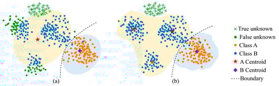
Figure 1. The illustration of open-set classification under varying intra-class multimodal perception capabilities. (a) Method that does not consider intra-class multimodal distribution. (b) Method that models the intra-class multimodal distribution.

Bayesian neural networks (BNNs) replace fixed weights with probability distributions and perform posterior inference within the Bayesian framework, offering a flexible and effective means to model the underlying data distribution while naturally representing predictive uncertainty. By explicitly capturing parameter uncertainty, BNNs can reduce reliance on specific fixed parameter values, leading to more robust predictions. Leveraging these advantages, numerous methods based on BNN have been designed for HSI classification, primarily under a closed-set setting [44,45]. For example, Haut et al. [44] employed Monte Carlo Dropout, in which dropout layers are treated as Bernoulli-distributed random variables. This allows training to approximate variational inference, enabling the model to capture the underlying data distribution and estimate predictive uncertainty. The obtained predictive uncertainty can then be used to filter high-quality samples, enhancing overall classification performance. Similarly, Preston et al. [45] utilized Monte Carlo Dropout to approximate variational inference, generating Bayesian posterior distributions and providing insight into predictive uncertainty. However, existing research has largely overlooked the potential of uncertainty-aware methods based on BNNs for open-set hyperspectral classification. Moreover, most BNNs relying on variational inference typically assume unimodal intra-class distributions, neglecting the potential multimodal structure within each class. This simplification restricts the model’s capability to model the global distribution of the data, particularly subtle intra-class variations in hyperspectral imagery, thereby limiting its effectiveness in open-set HSI classification.

To overcome the above challenges, an innovative open-set HSI classification framework, called the GDAN, is developed to enhance the model’s awareness of global distribution by performing fine-grained modeling of intra-class multimodal distributions (as shown in Figure 1b). First, this study adopts a GAN-based backbone and integrates an SA module to improve the model’s capacity for capturing long-range dependencies among the extensive spectral bands in hyperspectral data. Then, the fixed weights of the traditional discriminator in GAN are redefined as probability distributions, enabling posterior inference via MCMC sampling. This formulation enables the model to better capture intra-class multimodal structure and quantify predictive uncertainty. Consequently, the proposed model can form more precise boundaries separating known from unknown classes, and leverage uncertainty awareness to reliably separate unknown samples, thereby achieving accurate open-set HSI classification. The contributions are summarized as follows:

(1)

A novel Global Distribution-Aware framework for accurate open-set HSI classification is designed.

(2)

An interpretable model that integrates GAN and MCMC within a Bayesian framework is formed to explore complex multimodal distribution patterns in hyperspectral data.

(3)

The uncertainty modeling capability of the Bayesian framework is introduced into open-set HSI classification for the first time, providing a precise and reliable approach to the task.

2. Methodology

In this section, the proposed GDAN model is described in detail. First, the GAN is reinterpreted from a Bayesian perspective for open-set HSI classification. Then, the GAN and MCMC sampling are integrated within a unified Bayesian framework. Finally, a novel uncertainty-aware criterion is introduced to distinguish unknown samples from known classes. Figure 2 illustrates the structure of the proposed GDAN designed for open-set HSI classification.

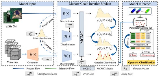
Figure 2. Overview of the proposed method. The objective function includes a Generator loss and a Discriminator loss, where the discriminator loss includes classification loss, prior loss, and noise gradient loss.

2.1. Global Distribution-Aware GAN

In GAN-based classification tasks, the original binary discriminator is typically replaced with a multiclass classifier, such as a softmax layer. Benefiting from the generator’s ability to accurately characterize class features, GAN-based classification methods often achieve satisfactory performance. However, the substantial number of spectral channels in hyperspectral data poses a challenge for the generator to capture long-range dependencies across these bands. Therefore, it is crucial to consider the band dependencies for a better exploration of the global distribution patterns in data.

To tackle this issue, this study incorporates an SA module into the generator, yielding the following output:

$$x_g=Attention\left(G\right(\mathcal{z};{\theta }_g\left)\right)$$

(1)

where $x_g$ is the generated samples of the generator $G$, and the noise $\mathcal{z}\in {\mathbb{R}}^{w\times h\times C}$. To avoid potential model collapse and better explore data distribution pattern, the $\mathcal{z}$ consists of a three-dimensional random noise cube $r\in {\mathbb{N}}^{w\times h\times c}$ with class labels $y\in {\mathsf{{\rm Y}}}^{w\times h\times P}$, where $c$ denotes the number of spectral channels, and $P$ indicates the number of classes. Also, $Attention(·)$ denotes the SA mechanism:

$$Attention\left(Q,K,V\right)=softmax\left({\displaystyle \frac{Q{K}^T}{\sqrt{d}}}\right)·V$$

(2)

For a given intermediate feature map $F$ from the generator, three parameterized matrices $W_Q$, $W_K$, $W_V$ are utilized to project $F$ into query, key and value space:

$$Q=F{W}_Q, K=F{W}_K, V=F{W}_V$$

(3)

Here, $Q$ specifies which contextual dependencies should be attended to, $K$ encodes the key features for similarity computation, and $V$ provides the feature content to be aggregated. The scaling factor $\sqrt{d}$ normalizes the dot product to stabilize training. Moreover, the generator can produce latent representations that resemble known class samples during training, and these representations assist in inferring the potential distribution of unknown classes that may exist.

To comprehensively model intra-class multimodal global distributions of HSI data, this study replaces the discriminator’s fixed weights with probability distributions and performs posterior inference within a Bayesian framework, guided by the conditional posterior distribution:

$$\begin{gathered} p\left({\theta }_d|X,Y,\mathcal{Z},{\theta }_g\right)\propto {\displaystyle \frac{1}{\left|n_d\right|}}(\prod _{i\in \left|n_d\right|}D\left(x_r^{\left(i\right)}=y_p^{\left(i\right)};{\theta }_d\right)·D(x_g^{\left(i\right)} \\ \hspace{1em}\hspace{1em}\hspace{1em} =\left[{\displaystyle \frac{1}{P}},{\displaystyle \frac{1}{P}},\dots ,{\displaystyle \frac{1}{P}}\right];{\theta }_d))·p\left({\theta }_d\right) \end{gathered}$$

(4)

where $x_r^{\left(i\right)}$ denotes the real sample. $y_p^{\left(i\right)}$ denotes the corresponding label, and $\left|n_d\right|$ is the numbers of mini-batch samples for the discriminator. In this way, we can introduce an uncountably infinite space over the weight distributions of the discriminator, which corresponds to every possible value of the data distribution. Specifically, given a dataset $\mathbb{Q}=\left\{x^{\left(i\right)}\right\}$ of variables $x^{\left(i\right)}~p_{data}\left(x\right)$, we can utilize a discriminator $D(x;{\theta }_d)$, parametrized by ${\theta }_d$ that samples from the posterior distribution, to output the probability that $x$ comes from the data distribution. By iteratively executing the above process, the probability distribution of each prediction can be estimated, thus obtaining both the class and the predictive uncertainty of the sample $x^{\left(i\right)}$. The backbone of the generator and discriminator is shown in Figure 3. Furthermore, it can be observed that the update of the discriminator is implicitly conditioned on the noise $\mathcal{Z}$ from Equation (4), thus the posterior of the discriminator can be further represented through marginalizing the noise $\mathcal{Z}$:

$$\begin{gathered} p\left({\theta }_d|X,Y,{\theta }_g\right)=\int p\left({\theta }_d|\mathcal{Z},{X,Y,\theta }_g\right)p\left(\mathcal{Z}|X,Y,{\theta }_g\right)d\mathcal{Z} \\ \hspace{1em}\hspace{1em}\hspace{1em}\hspace{1em} \approx {\displaystyle \frac{1}{\left|n_s\right|}}\sum _{i\in \left|n_s\right|}p\left({\theta }_d\right|{\mathcal{Z}}^{\left(i\right)},X,Y,{\theta }_g) \end{gathered}$$

(5)

where each ${\mathcal{Z}}^{\left(i\right)}$ has $n_d$ samples $\mathcal{z}$, $\left|n_s\right|$ represents the number of Monte Carlo (MC) samples for the discriminator. That is, the discriminator’s posterior distribution can be further represented with the sample set $\mho ={\left\{{\theta }_d^{\left(i\right)}\right\}}_{i=1}^{\left|n_s\right|}$, and each sample ${\theta }_d^{\left(i\right)}$ corresponds to the sampled noise ${\mathcal{Z}}^{\left(i\right)}$.

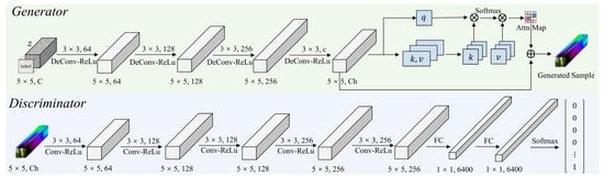
Figure 3. The backbone of the generator and discriminator.

2.2. Posterior Inference and Model Optimization

In Section 2.1, the discriminator is reformulated within a Bayesian framework, and the capability of the improved GAN to characterize global distribution is demonstrated. Nevertheless, two key challenges still remain. First, standard MC sampling, which relies on independent and identically distributed samples, may fail to sufficiently explore the complex multimodal distribution of the data, because it cannot fully capture the inherent correlations. Second, the effective inference of the discriminator’s posterior distribution in Equation (5) remains an open issue. To address these challenges, MCMC sampling offers a viable solution, as its iterative sample dependencies are well-suited for modeling complex intra-class multimodal distributions. In particular, Stochastic Gradient Hamiltonian Monte Carlo, a variant of MCMC, can take advantage of gradient information and use Hamiltonian dynamics simulations to sample the weight, enabling more efficient exploration of the parameter space [46]. The algorithm of the stochastic gradient Hamiltonian Monte Carlo can be expressed as follows:

$$\left\{\begin{array}{c}∆\theta =v_t\\ v_t=\left(1-\alpha \right)v_{t-1}-\eta \nabla \tilde{U}\left(x\right)+N\left(\mathrm{0,2}\left(\alpha -\widehat{\beta }\right)\eta \right)\end{array}\right.$$

(6)

where $\theta$ represents model parameters, $∆\theta$ denotes the update applied to the parameters at each iteration, $v_t$ is the momentum at iteration $t$, $v_{t-1}$ is the momentum from the previous iteration, $\alpha$ is the friction coefficient controlling momentum decay, $\eta$ denotes the step size, $\nabla \tilde{U}\left(x\right)$ represents the stochastic gradient, and $\mathcal{N}\left(\mathrm{0,2}\left(\alpha -\widehat{\beta }\right)\eta \right)$ is Gaussian noise with mean zero and variance $2\left(\alpha -\widehat{\beta }\right)$, where $\widehat{\beta }$ estimates the variance of the stochastic gradient noise. It can be observed that Equation (6) shares a clear correspondence with momentum-based Stochastic Gradient Descent (SGD). When compared with the SGD with momentum, it is evident that the parameter $\eta$ can correspond to the learning rate, while 1 − $\alpha$ corresponds to the momentum term. When the noise term $\mathcal{N}$ is excluded, the algorithm naturally reduces to standard SGD with momentum. Therefore, by additionally considering the influence of noise term $n$ during model updates, the SGD with momentum can thus be integrated into our model to update the sample set $\mho ={\left\{{\theta }_d^{\left(i\right)}\right\}}_{i=1}^{\left|n_s\right|}$, as we can calculate the loss gradient relative to the parameter that we are sampling:

$$\left\{\begin{array}{c}{\theta }_d^{\left(i\right)}={\theta }_d^{\left(i\right)-}+∆\theta ={\theta }_d^{\left(i\right)-}+v_t\\ v_t=\left(1-\alpha \right)v_{t-1}-\eta \nabla \tilde{U}\left(x\right)+n\end{array}\right.$$

(7)

where $n$ denotes the noise gradient caused by the stochastic gradient estimates of Hamiltonian dynamics simulation. Through the application of MCMC, the updated sample set $\mho ={\left\{{\theta }_d^{\left(i\right)}\right\}}_{i=1}^{\left|n_s\right|}$ can represent posterior distribution more accurately, while the discriminator’s posterior distribution in Equation (5) can also be inferred through Equation (7) directly. In this way, the GAN and MCMC are integrated within a new Bayesian framework, allowing the global data distribution to be modeled by exploring intra-class multimodal structures. For the proposed GDAN, the overall optimization procedure follows that of a traditional GAN, where training is guided by the adversarial interplay between the generator and the discriminator. Specifically, the GDAN’s objective function can be formulated as:

$${\mathcal{L}}_{GDAN}\left(G,D\right)=\underset{G}{min} \underset{D}{max}\left({\mathcal{L}}_g+{\mathcal{L}}_d\right)$$

(8)

where the generator loss ${\mathcal{L}}_g$ encourages the generator to produce class-specific samples that align with the given labels, while the discriminator loss ${\mathcal{L}}_d$ drives the discriminator to explore complex multimodal distribution patterns in the hyperspectral data, thereby enabling highly accurate HSI classification. It is worth noting that the generator is utilized solely during the training phase to facilitate adversarial learning and to model the latent feature distribution. During inference, the generator is not involved.

As mentioned above, the posterior sample set $\mho ={\left\{{\theta }_d^{\left(i\right)}\right\}}_{i=1}^{\left|n_s\right|}$ of the discriminator can be updated using momentum SGD with an additional noise term $n$. Accordingly, the discriminator loss ${\mathcal{L}}_d$ comprises three components: a classification loss, a prior loss, and an additional noise loss caused by the stochastic gradient estimates of Hamiltonian dynamics simulation:

$${\mathcal{L}}_d={\mathcal{L}}_d^{cla}+{\mathcal{L}}_d^{pri}+{\mathcal{L}}_d^{noi}$$

(9)

Specifically, classification loss ${\mathcal{L}}_d^{cla}$ is defined by the following equation:

$${\mathcal{L}}_d^{cla}={\left\{-{\displaystyle \frac{1}{\left|n_d\right|}}{\sum }_{i\in \left|n_d\right|}{\sum }_{p\in \left|P\right|}{y}_p^{\left(i\right)}\log D\left(x_r^{\left(i\right)};{\theta }_d^{\left(j\right)}\right)+y_g^{\left(i\right)}\log D\left(x_g^{\left(i\right)};{\theta }_d^{\left(j\right)}\right)\right\}}_{j=1}^{\left|n_s\right|}$$

(10)

where $y_g$ denote the class labels of the fake samples. And the prior loss ${\mathcal{L}}_d^{pri}$ is given by:

$${\mathcal{L}}_d^{pri}={\left\{{\displaystyle \frac{1}{\left|n_d\right|}}·{\displaystyle \frac{1}{\left|n_p\right|}}{\sum }_{i\in \left|n_p\right|}{\left({\displaystyle \frac{{\theta }_{di}^{\left(j\right)}}{\rho }}\right)}^2\right\}}_{j=1}^{\left|n_s\right|}$$

(11)

where $\left|n_p\right|$ indicates the total parameter number in ${\theta }_d$, and $\rho$ is the prior standard deviation. Moreover, the noise loss ${\mathcal{L}}_d^{noi}$ is computed as:

$${\mathcal{L}}_d^{noi}={\left\{{\displaystyle \frac{1}{\left|n_d\right|}}\sum {\theta }_d^{\left(i\right)}·n\right\}}_{i=1}^{\left|n_s\right|}$$

(12)

Correspondingly, the loss function of the generator can be formulated as:

$${\mathcal{L}}_g={\left\{{\displaystyle \frac{-1}{\left|n_d\right|}}{\sum }_{i\in \left|n_d\right|}{\sum }_{p\in \left|P\right|}{y}_p^{\left(i\right)}\log D(x_g^{\left(i\right)};{\theta }_d^{\left(j\right)})\right\}}_{j=1}^{\left|n_s\right|}$$

(13)

In Equation (10), the first term encourages the discriminator to assign higher probabilities to the true class, while the second term seeks to identify fake samples by assigning zero probability to all classes (i.e., the class probability is $\left[\mathrm{0,0},\dots ,0\right]$). However, the sum of the probabilities from the softmax layer is always 1. Therefore, the label $y_g=\left[\mathrm{0,0},\dots ,0\right]$ can be replaced with $y_g=\left[{\displaystyle \frac{1}{P}},{\displaystyle \frac{1}{P}},\dots ,{\displaystyle \frac{1}{P}}\right]$, which approximately treats fake samples as not belonging to any specific class. By iteratively sampling from the discriminator’s posterior distribution according to Equation (5), and training as specified in Equation (8), we can obtain an updated sample set $\mho ={\left\{{\theta }_d^{\left(i\right)}\right\}}_{i=1}^{\left|n_s\right|}$ from the approximate posterior over the weight of the discriminator. This strategy enables a more intuitive and straightforward inference of the posterior distribution, offering the advantage of not being restricted by the specific data distribution. As a result, it facilitates a more comprehensive exploration of the global data distribution, obtaining more accurate decision boundaries. Moreover, it should be noted that the generator receives feedback from multiple discriminators corresponding to different samples in $\mathrm{\mho }$, which means that the generator must fool all discriminators. This enables the generator to effectively explore distribution patterns of the data, and in turn guides the discriminator to better infer posterior distribution and further accelerate its convergence speed.

2.3. Uncertainty-Aware Open-Set HSI Classification

Benefiting from the inherent strength of the Bayesian posterior for uncertainty quantification, this paper develops an improved uncertainty metric, founded on precision global distribution modeling, to reliably identify unknown class. Specifically, the class probability $p\left(y^{\left(k\right)}\right)$ of the test data $x_{test}$ and the improved uncertainty can be determined by the sample set $\mathrm{\mho }$ as follows:

$$p(y^{\left(p\right)})={\displaystyle \frac{1}{\left|n_s\right|}}{\sum }_{i=1}^{\left|n_s\right|}p\left(y_p^{\left(i\right)}\right|x_{test},{\theta }_d^{\left(i\right)})$$

(14)

$$Uncertainty={\displaystyle \frac{-{\sum }_{p=1}^{P}p\left(y^{\left(p\right)}\right){\log }_{2}p\left(y^{\left(p\right)}\right)}{\underset{p}{\max }{\sum }_{i=1}^{\left|n_s\right|}\mathcal{l}}}$$

(15)

where the predictive uncertainty is quantified by incorporating both the entropy and the logits information, and $\mathcal{l}$ indicates the network’s output logits, and $\underset{p}{\max }\left(\right)$ denotes the operation that selects the logits corresponding to the output class. In this formulation, the obtained predictive uncertainty will take the logits into account, which can be seen as assigning mass (larger mass means that the model collected more evidence on a particular class) to all classes, rather than just the entropy that is calculated by the class probability of the model output. This is particularly important because the softmax function may map logits of different magnitudes to the same class probability, potentially obscuring differences in the model’s confidence across samples. For example, logits $[\mathrm{10,0},0]$ and $[5,-3,-3]$ may both yield softmax probabilities very close to $[\mathrm{1,0},0]$, despite the model having accumulated significantly stronger evidence (higher confidence) in the first case than in the second. Therefore, even if two samples exhibit similar predictive entropy (or even the same maximum softmax probability), the one with a larger logits should be treated as more certain (i.e., more likely to belong to a known class). Also, to facilitate intuitive and convenient comparisons between different methods, we normalized the uncertainty values. Then, a coefficient $\mathcal{w}$ is utilized to distinguish the unknown class from the known class, which can be computed using the uncertainty threshold $ϵ$:

$$\mathcal{w}=\left\{\begin{array}{c}1, if Uncertainty<ϵ\\ 0, if Uncertainty>ϵ\end{array}\right.$$

(16)

where ‘0’ and ‘1’ indicate the unknown and known classes, respectively. The open-set HSI classification results, ${\mathcal{C}}_{open}$, can be computed as:

$${\mathcal{C}}_{open}=\mathcal{w}⨀{\mathcal{C}}_{close}$$

(17)

where ${\mathcal{C}}_{close}$ denotes closed-set classification results.

3. Experiments

3.1. Dataset Description

(1) University of Pavia: The Pavia dataset was acquired by the ROSIS (Reflective Optics System Imaging Spectrometer) sensor over the University of Pavia in northern Italy, covering an area of 610 × 340 pixels with a spatial resolution of 1.3 m. The sensor captures 115 spectral bands spanning wavelength from 0.43 $\mathsf{\mu }\mathrm{m}$ to 0.86 $\mathsf{\mu }\mathrm{m}$. During preprocessing, 12 bands affected by water absorption and noise were removed, leaving 103 channels for analysis. Nine land cover classes were ultimately identified in the image. In Figure 4, we present the pseudo-color composite image, the ground truth image, and the corresponding color legend of the Pavia dataset.

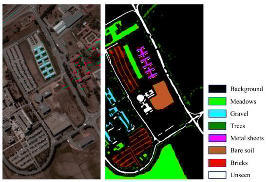
Figure 4. Pseudo-color composite image of the University of Pavia dataset, the corresponding ground truth, and legend.

(2) WHU-Hi-LongKou: The WHU-Hi-LongKou dataset was collected on 17 July 2018, over Longkou Town in Hubei province, China, using a Headwall Nano-Hyperspec imaging sensor with an 8 mm focal length mounted on a DJI matrix 600 Pro UAV [47]. The imagery has a resolution of 550 × 400 pixels, comprises 270 bands spanning 400 nm to 1000 nm, and offers a spatial resolution of approximately 0.463 m. The dataset defines a total of nine object classes. An overview of the dataset is provided in Figure 5.

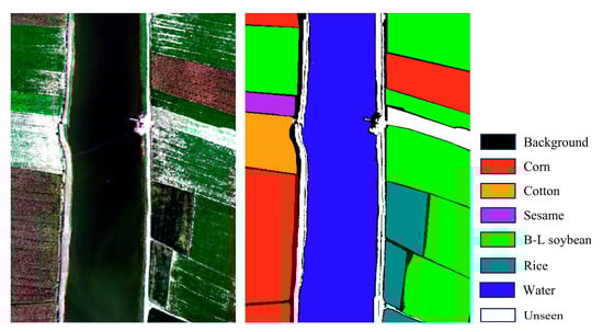
Figure 5. Pseudo-color composite image of the WHU-Hi-LongKou dataset, the corresponding ground truth, and legend.

(3) Salinas Valley: This image was collected by the airborne visible infrared imaging spectrometer (AVIRIS) sensor over Salinas Valley, CA, USA. It has a resolution of 512 × 217 pixels, with a spatial resolution of 3.7 m, and includes 224 bands covering the wavelength range from 0.4 $\mathsf{\mu }\mathrm{m}$ to 2.5 $\mathsf{\mu }\mathrm{m}$. In practice, 20 water absorption bands were removed, leaving 204 bands for analysis. The area contains sixteen distinct land-cover classes. Details of the dataset can be found in Figure 6.

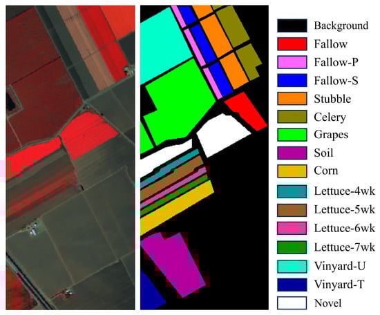
Figure 6. Pseudo-color composite image of the Salinas dataset, the corresponding ground truth, and legend.

To assess the effectiveness of the designed method in the open-set HSI classification task, several classes were designated as novel classes for each hyperspectral dataset. In the Pavia dataset, three classes—Asphalt, Bitumen, and Shadow—were treated as novel class. In the case of the WHU-Hi-LongKou dataset, the novel class comprised Cotton, Roads-Houses, and Mixed weed. In the Salinas dataset, two classes—weeds_1 and weeds_2—were selected as the novel class.

3.2. Experimental Setting

During the experiments, a random subset of labeled samples from each HSI dataset was chosen for training. For each dataset, the model was trained with varying numbers of samples per class—100 and 200, denoted as T = 100 and T = 200, where T represents the sample count. Each input HSI sample was assigned a spatial size of 5 × 5 pixels. During training, the experiments employed a batch size of 128, with training conducted over 3000 epochs for each dataset. To accelerate convergence, the SGD step was temporarily replaced with the Adam optimizer for the first 500 iterations, then reverted to SGD-based Stochastic Gradient Hamiltonian Monte Carlo. The initial learning rates assigned to the generator across the three datasets (Pavia, WHU-Hi-LongKou and Salinas) were set to $2.5\times {10}^{-5}$, $2.0\times {10}^{-5}$ and $5\times {10}^{-5}$, respectively. Correspondingly, the initial learning rates assigned to the discriminator for the three datasets were set to $1\times {10}^{-4}$, $1\times {10}^{-4}$ and $3\times {10}^{-4}$, respectively. For Stochastic Gradient Hamiltonian Monte Carlo, the learning rate for the discriminator was configured as $5\times {10}^{-5}$ with a momentum of 0.5. All experiments were conducted on a server running CentOS 7.6, equipped with an Intel (R) Xeon (R) Gold 5118 CPU, and an NVIDIA Tesla 100 16G GPU. Moreover, all deep learning models were implemented in Tensorflow (version 1.14.0) using Python 3.7.3. All experiments were independently repeated three times with different random seeds, and the mean and standard deviation of the results are reported. For the discriminative coefficient, the uncertainty threshold $ϵ$ was fixed at 0.5 and applied consistently across all datasets to identify unknown samples.

To evaluate the advantage of the designed method for open-set HSI classification, several advanced open-set HSI classification methods were included for comparison, including spectral–spatial latent recognition (SSLR) [34], a spectral–spatial multiple layer perceptron (MLP)-like network with reciprocal points learning (SSMLP) [48], a spatial-spectral selective transformer (HyperTaFOR) [40], and fractional-domain information-enhanced hyperspherical prototype learning (FrHSPL) [33]. To assess the superiority of the proposed method relative to traditional BNNs in global distribution perception and uncertainty modeling, a BNN-based HSI classification method called BDL-$G^2$-BFL (BDL-$G^2$) [49] is also used to carry out closed-set classification and uncertainty-aware unknown class identification. Furthermore, we also chose two outstanding closed-set HSI classification method called spectral–spatial adaptive Mamba (HyperMamba) [50], and MixerSENet [51]. The experimental results of all the comparison methods were obtained using their source codes or model structures. To ensure fairness and optimal performance in the context of this study, the implementations were fine-tuned, and their parameters were carefully adjusted.

To evaluate the performance of the proposed method against other state-of-the-art methods in open-set HSI classification, three metrics were used: Overall Accuracy ($OA$), Average Accuracy ($AA$), and Kappa Coefficient ($K$).

4. Experimental Results and Analysis

4.1. Ablation Experiment

To assess the contribution of key components in the proposed GDAN method, ablation studies were performed by selectively removing or substituting individual modules and examining their effects on open-set HSI classification. The proposed method is primarily composed of three core components: the SA module, the global distribution modeling module (GDM), and the improved uncertainty quantification module (UQ). For a fair comparison, the three parts were replaced with baseline alternatives while keeping other hyperparameters and training settings consistent. Specifically, in the variant without SA, the SA module in the generator is replaced with a stack of three-dimensional convolutional layers to test the necessity of SA in modeling spectral dependencies. In the variant without GDM, the MCMC-based global distribution modeling is replaced with Monte Carlo Dropout (MC Dropout), a common approximate Bayesian inference method. Here, Dropout layers with a rate of 0.3 are added to the discriminator, and uncertainty is estimated by performing 10 forward passes during testing to approximate the posterior distribution, akin to variational inference in traditional BNNs. This variant tests GDM’s contribution to handling complex intra-class multimodal distributions and unknown class identification. Moreover, in the variant without the UQ module, the quantification of prediction uncertainty does not take into account the effect of the output logits on the results. Experiments were conducted on the three datasets using 100 training samples per class. And performance was evaluated using $OA$, $AA$, $Kappa$, and unknown class ($Uc$) identification accuracy.

Table 1 presents the performance improvements in open-set HSI classification achieved by the proposed modules. According to the quantitative results in the first four rows, it can be observed that the GDM plays a more important role in improving the classification performance in all three datasets, and the UQ part is more significant than the SA. After that, it is not easy to find an optimal combination of these three components until jointly applying them, which reveals the importance of jointly adopting SA, GDM, and UQ. The ablation studies have clearly shown that these three key components substantially enhance the open-set classification accuracy, and GDAN is further optimized when these three components are employed together.

Table 1. Ablation results (%) of the proposed modules with T = 100 samples on three datasets.

Module			University of Pavia				WHU-Hi-LongKou				Salinas
SA	GDM	UQ	$OA$	$AA$	$K$	$Uc$	$OA$	$AA$	$K$	$Uc$	$OA$	$AA$	$K$	$Uc$
×	×	×	84.99	89.00	80.18	53.01	87.99	83.28	84.11	35.87	85.11	90.73	83.45	42.37
✓	×	×	85.33	89.24	80.62	54.67	88.38	83.80	84.62	37.24	86.00	91.29	84.44	50.81
×	✓	×	88.43	91.25	84.60	71.24	90.55	87.82	87.60	67.62	88.42	92.82	97.09	72.99
×	×	✓	87.13	90.47	82.93	63.27	89.71	86.32	86.46	57.14	87.08	91.97	85.62	61.01
✓	✓	×	89.71	92.24	86.29	75.66	90.76	88.17	87.88	70.14	88.94	93.19	87.67	74.91
✓	×	✓	88.90	91.57	85.21	73.50	90.36	87.48	87.34	65.26	87.61	92.30	86.20	65.98
×	✓	✓	90.64	92.76	87.48	81.86	91.46	88.91	88.78	68.89	89.74	93.69	88.56	82.44
✓	✓	✓	90.81	91.61	87.71	84.91	92.11	90.41	89.61	73.11	90.41	94.91	89.31	89.61

4.2. Results and Analysis

4.2.1. Classification Results on the University of Pavia Dataset

Table 2 and Table 3 report the $OA$, $AA$ and $Kappa$ values under the settings of 100 and 200 training samples per class, respectively. Overall, experimental results show that the proposed method surpasses the advanced closed-set HSI classification method under an open-set scenario, as measured by $OA$, $AA$, and the $Kappa$ coefficient. Specifically, with T = 100, our method outperforms the HyperMamba method, with gains of 16.6%, 11.6%, and 22.0%, respectively. Compared with the MixerSENet method, the $OA$, $AA$, and the $Kappa$ of the proposed GDAN increase by 16.3%, 10.7%, and 21.4%, respectively. When 200 samples per class are used, the proposed method achieves further gains of 20.0%, 13.7%, and 26.3%, respectively, over the HyperMamba method. And compared with the MixerSENet method, the $OA$, $AA$, and the $Kappa$ of the GDAN increase by 19.8%, 13.8%, and 26.0%, respectively. Moreover, it is evident that traditional closed-set HSI classification methods are incapable of identifying unknown class, primarily due to their dependence on pre-defined categories. In contrast, the proposed method exhibits robust performance in identifying unknown classes, achieving accuracies of 84.9% and 94.4% for the respective sample sizes, while preserving strong accuracy on the known classes.

Table 2. Classification results (%) by using 100 samples on the University of Pavia dataset.

Class	T = 100
	HyperMamba	MixerSENet	BDL-${\mathit{G}}^2$	SSLR	SSMLP	HyperTaFOR	FrHSPL	Ours
1	97.9 ± 0.9	95.1 ± 0.6	85.7 ± 0.9	93.4 ± 0.9	89.6 ± 1.7	89.2 ± 1.8	93.6 ± 1.1	93.2 ± 0.7
2	88.6 ± 1.6	94.7 ± 0.6	73.2 ± 1.2	91.3 ± 1.4	93.6 ± 0.7	73.9 ± 1.5	80.4 ± 2.4	89.3 ± 0.5
3	96.4 ± 0.7	96.4 ± 0.8	97.4 ± 0.6	96.5 ± 1.0	96.3 ± 1.0	98.4 ± 0.6	99.0 ± 0.5	95.9 ± 0.6
4	99.2 ± 0.4	99.6 ± 0.2	99.2 ± 0.3	99.4 ± 0.2	99.9 ± 0.1	99.8 ± 0.1	99.6 ± 0.2	98.9 ± 0.1
5	88.0 ± 1.6	87.9 ± 1.2	97.1 ± 0.6	77.4 ± 1.5	94.2 ± 0.4	97.6 ± 0.3	91.2 ± 0.4	90.7 ± 2.2
6	89.6 ± 1.8	92.6 ± 0.8	90.7 ± 0.6	88.8 ± 1.7	93.7 ± 1.2	95.3 ± 0.9	84.7 ± 1.2	88.3 ± 0.9
Novel	0.0 ± 0.0	0.0 ± 0.0	53.8 ± 0.7	49.9 ± 1.4	53.1 ± 0.9	74.4 ± 0.3	73.9 ± 0.2	84.9 ± 1.1
$OA$	74.2 ± 0.6	74.5 ± 0.4	81.5 ± 0.4	81.9 ± 0.7	83.4 ± 0.8	87.9 ± 1.0	88.4 ± 0.6	90.8 ± 0.4
$AA$	80.0 ± 0.6	80.9 ± 0.3	85.3 ± 0.3	85.2 ± 0.6	88.6 ± 0.3	89.8 ± 0.6	88.9 ± 0.5	91.6 ± 0.5
$K$	65.7 ± 0.8	66.3 ± 0.5	75.8 ± 0.4	75.8 ± 0.9	78.1 ± 0.9	84.0 ± 1.2	84.5 ± 0.7	87.7 ± 0.5

Table 3. Classification results (%) by using 200 samples on the University of Pavia dataset.

Class	T = 200
	HyperMamba	MixerSENet	BDL-${\mathit{G}}^2$	SSLR	SSMLP	HyperTaFOR	FrHSPL	Ours
1	95.7 ± 0.9	95.7 ± 0.8	91.4 ± 1.1	95.5 ± 1.2	97.6 ± 0.4	94.2 ± 0.7	93.0 ± 0.9	94.5 ± 0.8
2	90.8 ± 1.6	98.3 ± 0.3	79.7 ± 0.1	99.2 ± 0.4	93.4 ± 1.5	86.0 ± 1.9	92.7 ± 0.7	95.3 ± 1.0
3	97.5 ± 1.0	98.5 ± 0.4	95.6 ± 0.5	98.3 ± 0.4	96.8 ± 0.5	97.9 ± 0.2	98.1 ± 0.5	98.1 ± 0.6
4	99.8 ± 0.1	99.9 ± 0.0	99.5 ± 0.3	99.6 ± 0.2	99.8 ± 0.1	99.3 ± 0.3	99.9 ± 0.1	99.9 ± 0.1
5	94.9 ± 1.1	83.7 ± 1.0	92.5 ± 0.9	84.9 ± 2.6	96.6 ± 0.6	96.3 ± 0.3	99.2 ± 0.2	92.3 ± 1.3
6	93.6 ± 0.7	95.5 ± 0.6	77.4 ± 1.2	95.5 ± 1.2	95.3 ± 1.2	92.1 ± 1.0	94.8 ± 0.4	94.4 ± 0.6
Novel	0.0 ± 0.0	0.0 ± 0.0	66.1 ± 0.5	56.6 ± 1.5	68.2 ± 0.8	81.3 ± 0.3	80.7 ± 0.4	94.4 ± 0.8
$OA$	74.6 ± 0.6	74.8 ± 0.3	85.0 ± 0.4	86.2 ± 0.7	90.7 ± 0.4	91.6 ± 0.4	91.9 ± 0.4	94.6 ± 0.5
$AA$	81.8 ± 0.4	81.7 ± 0.2	86.0 ± 0.3	89.9 ± 0.6	92.5 ± 0.5	92.4 ± 0.4	94.0 ± 0.1	95.5 ± 0.2
$K$	66.4 ± 0.7	66.7 ± 0.3	80.1 ± 0.5	81.6 ± 1.0	87.4 ± 0.5	88.7 ± 0.5	89.2 ± 0.5	92.7 ± 0.6

As illustrated in Table 2 and Table 3, our method also surpasses the most advanced open-set HSI classification methods across superior classification performance in an open-set environment. With 100 samples per class, the $OA$, $AA$ and $Kappa$ of the proposed method increased by 8.9%, 6.4%, and 11.9%, respectively, over the SSEL method. Compared with the SSMLP method, the $OA$, $AA$, and the $Kappa$ of the GDAN increase by 7.4%, 3.0%, and 9.6%, respectively. Similarly, compared with the recently introduced HyperTaFOR and FrHSPL, the proposed method achieves consistent improvements. Specifically, it outperforms HyperTaFOR by 2.9%, 1.8%, and 3.7% in $OA$, $AA$, and $Kappa$, and surpasses FrHSPL by 2.4%, 2.7%, and 3.2%, respectively. With 200 samples per class, the proposed method continues to outperform all advanced open-set HSI classification methods, yielding performance gains ranging from 3.0% to 11.1% across $OA$, $AA$, and $Kappa$. Even when compared to the BNNs-based method BDL-$G^2$, which are recognized for their superior ability to model data distributions, our method continues to obtain the highest open-set classification accuracy. Notably, the proposed method also significantly surpasses these leading open-set HSI classification approaches in identifying unknown class, yielding improvements ranging from 10.5% to 37.8% across different sample proportions.

For illustration, Figure 7 presents the open-set HSI classification results generated by different methods for the Pavia dataset under different sample sizes. It can be observed that our method effectively identifies the unknown class, largely due to its global distribution modeling. Among the compared methods, only five open-set HSI classification methods are capable of identifying the unknown class, albeit with suboptimal performance. In contrast, the closed-set HSI classification method incorrectly assigns the unknown samples to known classes, reflecting their reliance on predefined ground classes. Furthermore, the results in Figure 7 illustrate that the proposed method not only effectively identifies unknown classes but also preserves high classification accuracy for the known classes.

Figure 7. Open-set HSI classification maps for the University of Pavia dataset. (a–h) 100-sample scenario. (i–p) 200-sample scenario. From left to right: HyperMamba, MixerSENet, BDL-$G^2$, SSLR, SSMLP, HyperTaFOR, FrHSPL, and ours.

4.2.2. Classification Results on the WHU-Hi-LongKou Dataset

For the second experiment on the WHU-Hi-LongKou dataset, Table 4 and Table 5 present the classification accuracies of the proposed method alongside the comparison methods. As shown in the table, our method achieves the highest performance in the open-set setting. Specifically, under the 100-sample scenario, the $OA$, $AA$ and $Kappa$ of our method improve by 4.8%, 7.7%, and 6.4%, respectively, compared with the advanced closed-set HSI classification method HyperMamba. Compared with the MixerSENet method, the $OA$, $AA$ and $Kappa$ of the GDAN method increased by 3.9%, 7.3%, and 5.2%. In the 200-sample scenario, our method continues to achieve superior classification accuracy in the open-set environment. Notably, both HyperMamba and MixerSENet fail to correctly identify the unknown class, whereas the proposed method successfully detects the unknown class with accuracies of 73.1% and 80.3% under different sample proportions.

Table 4. Classification results (%) by using 100 samples on the WHU-Hi-LongKou dataset.

Class	T = 100
	HyperMamba	MixerSENet	BDL-${\mathit{G}}^2$	SSLR	SSMLP	HyperTaFOR	FrHSPL	Ours
1	98.7 ± 0.4	98.3 ± 0.5	95.1 ± 1.1	99.6 ± 0.1	97.6 ± 0.8	95.1 ± 0.3	97.4 ± 0.5	97.1 ± 1.0
2	94.3 ± 1.2	98.0 ± 0.3	96.5 ± 0.5	78.6 ± 0.9	99.3 ± 0.3	99.6 ± 0.2	99.4 ± 0.3	88.3 ± 1.8
3	99.2 ± 0.6	96.8 ± 0.4	99.2 ± 0.3	72.1 ± 1.5	93.0 ± 0.9	92.7 ± 0.7	91.5 ± 0.8	91.7 ± 0.7
4	86.8 ± 1.0	89.4 ± 1.4	89.8 ± 1.4	85.4 ± 2.1	78.8 ± 1.8	87.3 ± 1.9	85.1 ± 2.1	85.8 ± 2.0
5	100.0 ± 0.0	99.6 ± 0.2	97.0 ± 0.9	95.5 ± 0.8	93.0 ± 1.1	90.0 ± 1.5	91.2 ± 0.5	97.5 ± 0.6
6	99.8 ± 0.1	99.9 ± 0.1	98.8 ± 0.3	98.2 ± 0.3	97.1 ± 0.4	99.6 ± 0.2	98.6 ± 0.5	99.6 ± 0.1
Novel	0.0 ± 0.0	0.0 ± 0.0	53.9 ± 1.8	43.3 ± 1.4	51.6 ± 1.5	63.5 ± 0.3	57.4 ± 0.6	73.1 ± 1.0
$OA$	87.3 ± 0.3	88.2 ± 0.4	91.6 ± 0.4	88.7 ± 0.8	87.6 ± 0.6	91.4 ± 0.5	90.4 ± 0.7	92.1 ± 0.6
$AA$	82.7 ± 0.3	83.1 ± 0.3	90.0 ± 0.3	81.8 ± 0.5	87.2 ± 0.5	89.7 ± 0.2	88.6 ± 0.4	90.4 ± 0.5
$K$	83.2 ± 0.5	84.4 ± 0.6	88.9 ± 0.5	85.1 ± 1.0	83.9 ± 0.8	88.8 ± 0.6	87.4 ± 0.9	89.6 ± 0.8

Table 5. Classification results (%) by using 200 samples on the WHU-Hi-LongKou dataset.

Class	T = 200
	HyperMamba	MixerSENet	BDL-${\mathit{G}}^2$	SSLR	SSMLP	HyperTaFOR	FrHSPL	Ours
1	99.4 ± 0.3	99.4 ± 0.2	94.6 ± 1.2	98.9 ± 0.3	98.8 ± 0.5	91.7 ± 0.7	95.4 ± 0.7	95.7 ± 0.9
2	94.1 ± 0.4	98.3 ± 0.4	96.4 ± 0.7	79.4 ± 1.3	99.7 ± 0.1	99.8 ± 0.1	99.7 ± 0.2	90.5 ± 1.2
3	99.0 ± 0.4	98.5 ± 0.4	99.1 ± 0.2	94.4 ± 0.7	94.5 ± 1.6	98.6 ± 0.6	97.9 ± 1.0	91.1 ± 1.1
4	96.4 ± 0.8	97.9 ± 0.5	91.2 ± 1.4	91.3 ± 0.5	87.3 ± 0.8	90.0 ± 0.7	89.0 ± 0.6	86.0 ± 2.3
5	99.8 ± 0.2	99.6 ± 0.1	95.5 ± 1.8	96.4 ± 0.4	94.8 ± 1.0	92.0 ± 2.1	98.0 ± 0.9	99.3 ± 0.2
6	99.5 ± 0.3	99.4 ± 0.3	99.3 ± 0.2	95.9 ± 0.2	98.0 ± 0.9	99.7 ± 0.2	98.0 ± 0.7	99.5 ± 0.3
Novel	0.0 ± 0.0	0.0 ± 0.0	54.9 ± 1.7	46.2 ± 0.4	46.3 ± 1.6	64.8 ± 0.3	62.5 ± 1.5	80.3 ± 0.5
$OA$	90.2 ± 0.3	90.9 ± 0.1	92.0 ± 0.6	90.3 ± 0.2	90.5 ± 0.6	92.1 ± 0.3	91.9 ± 0.4	92.6 ± 0.7
$AA$	84.0 ± 0.1	84.7 ± 0.1	90.1 ± 0.6	86.1 ± 0.3	88.5 ± 0.5	90.9 ± 0.4	91.5 ± 0.4	91.8 ± 0.2
$K$	86.9 ± 0.4	87.9 ± 0.2	89.5 ± 0.8	87.3 ± 0.3	87.5 ± 0.7	89.6 ± 0.4	89.4 ± 0.5	90.4 ± 0.9

Table 4 and Table 5 further demonstrate that the proposed method consistently surpasses all four advanced open-set HSI classification methods in terms of open-set performance. For the case of T = 100, the proposed method achieves improvements ranging from 0.7% to 8.6% across $OA$, $AA$, and $Kappa$ compared with the competing methods. When the number of training samples increases to T = 200, the method maintains its superiority, yielding gains in the range of 0.3% to 5.7% over the four state-of-the-art baselines. Furthermore, the proposed method consistently surpasses the BNNs-based method BDL-$G^2$ across varying sample proportions. Notably, the proposed method markedly outperforms all leading open-set HSI classification methods in identifying unknown class, with improvements ranging from 9.6% to 34.1% across different sample proportions.

For illustration, Figure 8 presents the classification results produced by various methods for the WHU-Hi-LongKou dataset. These results demonstrate that our method obtains the best performance in identifying the unknown class. As observed on the WHU-Hi-LongKou dataset, the closed-set HSI classifiers still fail to identify the unknown class, instead assigning it to a known label. This limitation stems from the closed-set assumption, where all classes are predefined, which prevents the model from handling unknown class. While other open-set classification models can identify unknown class to some extent, their performance remains substantially inferior compared to that of the proposed method.

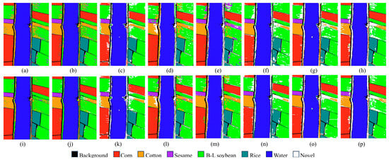
Figure 8. Open-set HSI classification maps for the WHU-Hi-LongKou dataset. (a–h) 100-sample scenario. (i–p) 200-sample scenario. From left to right: HyperMamba, MixerSENet, BDL-$G^2$, SSLR, SSMLP, HyperTaFOR, FrHSPL, and ours.

4.2.3. Classification Results on the Salinas Dataset

The Salinas dataset was employed in the third experiment, and Table 6 and Table 7 report the classification results for 100 and 200 samples per class. In the 100-sample context, the proposed method demonstrates outstanding open-set classification performance, with $OA$, $AA$ and $Kappa$ reaching 90.4%,94.9% and 89.3%, respectively. Additionally, the proposed method also excels in unknown class identification, achieving an accuracy of 89.6%, outperforming all comparison methods. Under the 200-sample scenario, the proposed method maintains the best open-set classification performance, with $OA$, $AA$ and $Kappa$ values of 94.8%, 97.6% and 94.1%, respectively. In terms of unknown class detection, the proposed method markedly surpasses the comparative methods, with improvements ranging from 19.8% to 33.2%. These results confirm that the proposed method performs well in both open-set classification and detecting unknown classes.

Table 6. Classification results (%) by using 100 samples on the Salinas dataset.

Class	T = 100
	HyperMamba	MixerSENet	BDL-${\mathit{G}}^2$	SSLR	SSMLP	HyperTaFOR	FrHSPL	Ours
1	99.7 ± 0.2	99.7 ± 0.1	99.7 ± 0.2	99.8 ± 0.1	97.5 ± 0.3	99.8 ± 0.2	97.7 ± 0.7	99.3 ± 0.2
2	99.4 ± 0.2	99.6 ± 0.2	99.1 ± 0.5	98.8 ± 0.4	98.7 ± 0.2	99.5 ± 0.2	96.1 ± 0.8	98.8 ± 0.3
3	98.8 ± 0.3	97.5 ± 0.3	97.1 ± 0.8	96.6 ± 0.3	93.7 ± 0.8	97.5 ± 0.3	98.7 ± 0.6	96.2 ± 0.7
4	99.6 ± 0.3	99.8 ± 0.2	98.5 ± 0.3	99.4 ± 0.3	98.9 ± 0.5	98.3 ± 0.5	97.6 ± 0.7	99.1 ± 0.2
5	99.1 ± 0.6	99.6 ± 0.2	95.7 ± 0.7	99.4 ± 0.2	98.6 ± 0.2	97.7 ± 0.6	99.8 ± 0.1	97.9 ± 0.5
6	71.5 ± 1.9	84.8 ± 2.4	85.5 ± 1.9	84.0 ± 2.6	83.7 ± 0.6	97.4 ± 0.6	75.5 ± 2.0	77.9 ± 1.7
7	99.1 ± 0.2	98.6 ± 0.4	97.7 ± 0.6	99.0 ± 0.5	91.0 ± 0.9	99.7 ± 0.1	99.1 ± 0.2	96.5 ± 0.4
8	88.5 ± 1.3	92.4 ± 1.8	99.5 ± 0.3	99.2 ± 0.2	79.8 ± 0.7	98.9 ± 0.3	99.7 ± 0.2	85.8 ± 1.4
9	99.6 ± 0.3	99.3 ± 0.2	89.5 ± 1.3	99.7 ± 0.2	92.3 ± 1.1	99.8 ± 0.1	99.8 ± 0.1	98.5 ± 0.3
10	99.6 ± 0.2	99.7 ± 0.2	94.2 ± 0.8	98.1 ± 0.6	99.2 ± 0.3	96.7 ± 0.6	99.3 ± 0.3	99.7 ± 0.2
11	99.3 ± 0.4	99.4 ± 0.2	99.7 ± 0.1	99.3 ± 0.2	98.6 ± 0.2	100.0 ± 0.0	99.5 ± 0.2	99.7 ± 0.1
12	96.9 ± 0.5	98.1 ± 0.6	98.4 ± 0.5	97.9 ± 0.5	92.3 ± 1.6	97.2 ± 0.6	96.7 ± 0.8	98.7 ± 0.3
13	81.2 ± 1.9	75.8 ± 0.8	70.7 ± 1.1	80.6 ± 1.5	76.8 ± 2.5	61.0 ± 0.9	89.9 ± 0.9	87.1 ± 2.4
14	99.4 ± 0.2	98.9 ± 0.3	69.8 ± 1.1	99.9 ± 0.0	97.5 ± 0.6	99.6 ± 0.2	100.0 ± 0.0	99.1 ± 0.5
Novel	0.0 ± 0.0	0.0 ± 0.0	57.0 ± 0.5	60.5 ± 0.4	68.1 ± 1.5	56.3 ± 0.3	72.0 ± 0.4	89.6 ± 0.5
$OA$	78.8 ± 0.6	82.1 ± 0.5	86.2 ± 0.5	89.3 ± 0.6	86.4 ± 0.5	88.9 ± 0.3	89.9 ± 0.5	90.4 ± 0.6
$AA$	88.8 ± 0.2	89.5 ± 0.2	90.1 ± 0.3	94.1 ± 0.2	91.1 ± 0.3	93.3 ± 0.2	94.8 ± 0.2	94.9 ± 0.3
$K$	76.5 ± 0.7	80.2 ± 0.5	84.7 ± 0.6	88.1 ± 0.7	84.8 ± 0.5	87.6 ± 0.3	88.8 ± 0.5	89.3 ± 0.7

Table 7. Classification results (%) by using 200 samples on the Salinas dataset.

Class	T = 200
	HyperMamba	MixerSENet	BDL-${\mathit{G}}^2$	SSLR	SSMLP	HyperTaFOR	FrHSPL	Ours
1	99.7 ± 0.1	99.8 ± 0.2	99.7 ± 0.2	99.3 ± 0.2	98.9 ± 0.3	99.8 ± 0.2	99.8 ± 0.1	99.5 ± 0.3
2	99.8 ± 0.1	99.9 ± 0.1	99.3 ± 0.3	98.9 ± 0.2	96.5 ± 0.9	98.7 ± 0.2	99.5 ± 0.2	99.0 ± 0.3
3	98.5 ± 0.3	98.1 ± 0.5	96.7 ± 0.4	96.8 ± 1.0	94.3 ± 0.4	96.6 ± 0.4	95.8 ± 0.8	99.7 ± 0.2
4	99.9 ± 0.1	99.5 ± 0.2	97.6 ± 0.6	99.5 ± 0.2	98.1 ± 0.5	99.1 ± 0.1	99.7 ± 0.1	99.7 ± 0.2
5	99.2 ± 0.3	99.4 ± 0.4	97.9 ± 0.7	98.8 ± 0.2	94.2 ± 0.6	98.9 ± 0.3	98.6 ± 0.2	99.2 ± 0.4
6	77.4 ± 1.8	84.6 ± 2.4	91.9 ± 0.8	86.9 ± 2.7	87.3 ± 2.3	86.4 ± 0.5	98.7 ± 0.7	85.3 ± 1.9
7	97.9 ± 0.3	98.2 ± 0.4	98.7 ± 0.5	98.7 ± 0.4	93.4 ± 0.7	99.0 ± 0.4	99.2 ± 0.2	98.3 ± 0.1
8	95.9 ± 0.8	99.6 ± 0.2	99.9 ± 0.0	98.8 ± 0.4	80.8 ± 0.7	99.7 ± 0.2	99.6 ± 0.2	96.1 ± 0.4
9	99.6 ± 0.2	97.5 ± 0.8	90.0 ± 0.7	99.6 ± 0.2	93.1 ± 0.6	100.0 ± 0.0	99.6 ± 0.1	99.3 ± 0.3
10	99.7 ± 0.1	99.3 ± 0.3	96.2 ± 0.8	99.7 ± 0.2	98.5 ± 0.3	98.1 ± 0.9	99.2 ± 0.3	99.8 ± 0.1
11	99.8 ± 0.2	98.4 ± 0.2	99.9 ± 0.1	99.8 ± 0.1	99.1 ± 0.3	100.0 ± 0.0	99.7 ± 0.1	99.3 ± 0.1
12	98.3 ± 0.3	98.4 ± 0.6	98.5 ± 0.4	98.8 ± 0.7	94.1 ± 0.9	97.0 ± 0.4	98.2 ± 0.5	99.7 ± 0.2
13	83.4 ± 1.5	85.6 ± 1.8	80.9 ± 1.0	89.7 ± 0.9	81.7 ± 1.1	85.2 ± 0.9	79.9 ± 1.5	91.3 ± 2.2
14	99.2 ± 0.2	99.1 ± 0.3	71.1 ± 1.8	99.7 ± 0.1	98.3 ± 0.5	100.0 ± 0.0	99.9 ± 0.1	99.4 ± 0.1
Novel	0.0 ± 0.0	0.0 ± 0.0	68.9 ± 0.4	64.7 ± 1.2	74.6 ± 0.6	78.1 ± 0.1	76.5 ± 0.4	97.9 ± 0.5
$OA$	80.7 ± 0.5	83.7 ± 0.6	90.5 ± 0.2	91.1 ± 0.5	88.7 ± 0.4	92.3 ± 0.2	94.0 ± 0.2	94.8 ± 0.6
$AA$	89.9 ± 0.2	90.5 ± 0.2	92.5 ± 0.1	95.3 ± 0.2	92.2 ± 0.2	95.8 ± 0.1	96.3 ± 0.1	97.6 ± 0.2
$K$	78.6 ± 0.6	82.0 ± 0.6	89.4 ± 0.2	90.1 ± 0.6	87.3 ± 0.5	91.4 ± 0.2	93.3 ± 0.2	94.1 ± 0.7

For illustrative purposes, Figure 9 presents the classification results obtained by various methods for the Salinas dataset. It is clear that existing methods, particularly the closed-set method, frequently misidentify unknown samples as known classes. Our method, however, correctly classifies unknown classes while maintaining strong performance on known classes, underscoring its effectiveness in addressing open-set classification challenges.

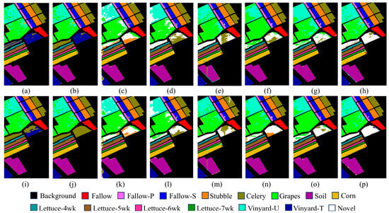
Figure 9. Open-set HSI classification maps for the Salinas dataset. (a–h) 100-sample scenario. (i–p) 200-sample scenario. From left to right: HyperMamba, MixerSENet, BDL-$G^2$, SSLR, SSMLP, HyperTaFOR, FrHSPL, and ours.

5. Discussion

5.1. Effectiveness of Global Distribution Modeling

To further evaluate the capability of the proposed method in modeling global distribution by exploring intra-class multimodal structures, two additional experiments were conducted under a 100-sample context.

In the first experiment, two classes (Gravel and Trees) with significantly different features were merged in the Pavia University dataset to simulate a more complex intra-class multimodal distribution within the class. The novel classes remain the same as in section A. As presented in Table 8, the proposed approach applied to the merged class achieves higher classification accuracy, demonstrating its ability to efficiently capture intra-class multimodal distribution patterns and extract representative features that characterize class information. Moreover, the proposed method consistently outperforms others in open-set HSI classification and unknown class identification. These results indicate that modeling the global data distribution pattern not only facilitates intra-class feature learning but also enhances inter-class boundary delineation, thereby enhancing the classification accuracy and the discrimination between known and unknown classes. To further demonstrate the effectiveness of the proposed method in exploring multimodal distribution, feature representations extracted by different methods were projected into 2D space using t-SNE on the Pavia dataset, as shown in Figure 10. The results indicate that the extracted features obtained by our method exhibit superior separability, while other methods show a clear mixture of different classes, particularly for the novel classes. More importantly, the projected features of the merged class extracted from our method are aggregated in the low-dimensional space, suggesting that the model can maintain consistent feature representation even for data with multimodal distributions but consistent labels. Meanwhile, the projected features of the subclasses within the merged class also exhibit discernible boundaries, indicating that the model can differentiate between distinct patterns within the data.

Table 8. Classification results (%) under multimodal distribution environment on the Pavia dataset.

Class	HyperMamba	MixerSENet	BDL-${\mathit{G}}^2$	SSLR	SSMLP	HyperTaFOR	FrHSPL	Ours
1	97.0 ± 0.5	93.3 ± 0.5	90.9 ± 0.8	97.4 ± 0.8	94.9 ± 1.4	90.5 ± 1.2	93.7 ± 1.0	96.6 ± 0.6
2	88.9 ± 1.4	89.5 ± 1.2	81.7 ± 1.0	90.9 ± 0.1	88.0 ± 1.1	87.2 ± 1.8	91.4 ± 1.0	92.4 ± 0.8
3	99.7 ± 0.1	99.9 ± 0.1	99.7 ± 0.1	99.6 ± 0.2	99.8 ± 0.2	99.6 ± 0.3	99.1 ± 0.2	100.0 ± 0.0
4	91.1 ± 1.4	90.2 ± 0.9	97.0 ± 1.0	98.9 ± 0.2	91.1 ± 1.0	97.0 ± 0.7	96.3 ± 0.3	94.8 ± 0.6
5	96.6 ± 0.5	97.7 ± 0.3	86.4 ± 0.5	91.3 ± 0.6	97.0 ± 0.9	86.3 ± 2.2	93.7 ± 0.9	95.3 ± 0.9
Novel	0.0 ± 0.0	0.0 ± 0.0	51.2 ± 1.4	42.1 ± 1.8	49.6 ± 0.5	73.1 ± 0.6	77.4 ± 0.5	83.8 ± 1.3
$OA$	74.3 ± 0.3	73.6 ± 0.2	81.8 ± 0.6	84.3 ± 0.6	84.1 ± 0.6	87.1 ± 0.7	90.5 ± 0.4	93.1 ± 0.4
$AA$	78.9 ± 0.4	78.4 ± 0.1	84.5 ± 0.3	86.7 ± 0.4	86.7 ± 0.2	88.9 ± 0.5	91.9 ± 0.2	93.8 ± 0.4
$K$	65.3 ± 0.4	64.8 ± 0.2	75.5 ± 0.7	78.7 ± 0.8	78.5 ± 0.8	82.7 ± 0.9	87.1 ± 0.5	90.6 ± 0.5

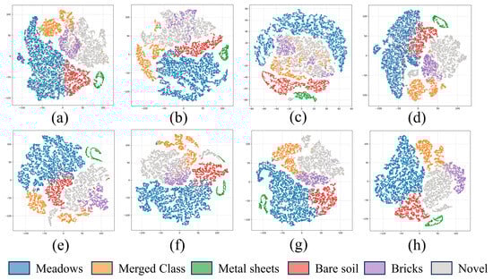
Figure 10. Feature visualization by t-SNE on the University of Pavia dataset. (a) HyperMamba. (b) MixerSENet. (c) BDL-$G^2$. (d) SSLR. (e) SSMLP. (f) HyperTaFOR. (g) FrHSPL. (h) Ours.

For the second experiment, four classes (Lettuce-4wk, Lettuce-5wk, Lettuce-6wk and Lettuce-7wk) that represent different growth stages of lettuce were merged in the Salians dataset to further simulate a complex intra-class multimodal distribution environment. Table 9 reports the open-set classification performance for the proposed and comparative methods, showing that our approach obtains the highest accuracy for the merged classes. This suggests that the proposed method can more effectively explore global distributions, and even complex multimodal distribution structures within merged classes. By accurately modeling these data distributions, the proposed method establishes clearer decision boundaries between known and unknown classes, thereby enabling more reliable identification of known classes. We also projected the feature representations acquired by different methods onto a 2D space using t-SNE on the Salinas dataset, as illustrated in Figure 11. The results indicate that the projected features of the merged class extracted by the proposed method form more compact clusters in the low-dimensional space compared with other approaches, while still preserving satisfactory separability among the subclasses within the merged class.

Table 9. Classification results (%) under multimodal distribution environment on the Salinas dataset.

Class	HyperMamba	MixerSENet	BDL-${\mathit{G}}^2$	SSLR	SSMLP	HyperTaFOR	FrHSPL	Ours
1	99.3 ± 0.3	92.2 ± 0.2	99.9 ± 0.1	99.0 ± 0.2	97.4 ± 0.5	99.3 ± 0.5	99.6 ± 0.2	100.0 ± 0.0
2	99.4 ± 0.1	99.8 ± 0.1	99.3 ± 0.3	99.3 ± 0.2	99.3 ± 0.3	90.6 ± 1.0	99.8 ± 0.1	99.4 ± 0.2
3	97.2 ± 0.6	99.1 ± 0.1	93.1 ± 1.0	95.3 ± 1.1	95.4 ± 0.9	98.2 ± 0.4	97.9 ± 0.3	98.2 ± 0.6
4	99.5 ± 0.2	99.8 ± 0.1	98.6 ± 0.7	99.7 ± 0.1	99.6 ± 0.2	99.5 ± 0.3	99.7 ± 0.2	99.7 ± 0.1
5	99.3 ± 0.2	98.2 ± 0.5	99.6 ± 0.2	99.0 ± 0.4	99.1 ± 0.3	99.7 ± 0.2	99.8 ± 0.1	97.6 ± 0.2
6	75.1 ± 2.1	84.8 ± 1.1	88.3 ± 1.6	87.4 ± 1.5	90.9 ± 1.9	94.2 ± 0.7	77.2 ± 1.3	84.5 ± 1.1
7	99.5 ± 0.2	98.8 ± 0.4	99.9 ± 0.1	91.8 ± 1.3	92.6 ± 1.5	99.7 ± 0.2	99.3 ± 0.1	99.2 ± 0.4
8	98.0 ± 0.9	95.2 ± 0.9	99.0 ± 0.2	97.3 ± 0.3	98.7 ± 0.2	99.6 ± 0.2	99.2 ± 0.4	98.7 ± 0.3
9	98.9 ± 0.4	98.6 ± 0.2	97.7 ± 0.6	97.3 ± 1.1	96.3 ± 0.4	98.1 ± 0.3	96.4 ± 1.0	99.4 ± 0.3
10	85.6 ± 1.1	72.3 ± 1.9	84.0 ± 1.4	93.2 ± 1.2	92.1 ± 0.9	72.6 ± 1.6	91.6 ± 0.8	89.5 ± 2.4
11	98.8 ± 0.5	98.6 ± 0.4	99.8 ± 0.1	98.1 ± 0.4	97.7 ± 0.4	99.4 ± 0.3	99.8 ± 0.1	97.4 ± 0.7
Novel	0.0 ± 0.0	0.0 ± 0.0	56.6 ± 1.6	65.5 ± 1.1	63.5 ± 1.1	76.6 ± 0.7	80.4 ± 0.4	87.9 ± 0.9
$OA$	80.7 ± 0.5	81.4 ± 0.2	89.6 ± 0.5	90.6 ± 0.4	91.0 ± 0.3	92.0 ± 0.4	91.4 ± 0.3	93.2 ± 0.4
$AA$	87.6 ± 0.2	86.5 ± 0.2	93.0 ± 0.3	93.6 ± 0.2	93.5 ± 0.2	93.9 ± 0.3	95.1 ± 0.2	96.0 ± 0.2
$K$	78.4 ± 0.5	79.3 ± 0.3	88.3 ± 0.6	89.4 ± 0.5	89.9 ± 0.3	91.0 ± 0.4	90.4 ± 0.4	92.4 ± 0.5

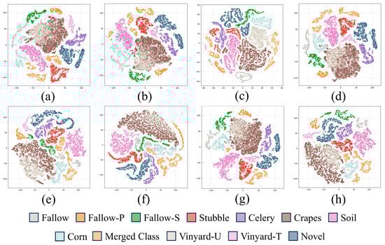
Figure 11. Feature visualization by t-SNE on the Salinas dataset. (a) HyperMamba. (b) MixerSENet. (c) BDL-$G^2$. (d) SSLR. (e) SSMLP. (f) HyperTaFOR. (g) FrHSPL. (h) Ours.

5.2. Visualization of the Uncertainty Modeling

Within the Bayesian framework, models inherently quantify predictive uncertainty, offering an indicator to distinguish known from unknown classes in open-set HSI classification. To assess the effectiveness of the proposed method relative to traditional BNNs, this section presents a comparative analysis of their performance in uncertainty modeling, using the results from the 200-sample setting, as reported in Table 3, Table 5 and Table 7.

To provide an intuitive illustration of the advantages of the proposed method in uncertainty modeling, we present the predictive uncertainty obtained by both the designed method and the BNNs-based method BDL-$G^2$ in Figure 12, Figure 13 and Figure 14. As shown in Figure 12, the proposed method exhibits a more refined capability for quantifying uncertainty across classification results under varying sample sizes. This enhancement stems from two main factors. First, the proposed global distribution modeling module allows the model to capture the true underlying data distribution more accurately. Second, the proposed improved uncertainty quantification module further incorporates the model’s confidence in the samples, effectively mitigating the biases associated with relying solely on individual computational metrics, and improving the precision and stability of recognition for unseen samples. In contrast, although BDL-$G^2$ are capable of quantifying predictive uncertainty to some extent, their ability to perceive complex data distributions and model uncertainty is limited, hindering the establishment of clear boundaries between known and unknown classes in the feature space.

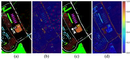
Figure 12. Open-set classification results and predictive uncertainty on the University of Pavia dataset. (a,b) BDL-$G^2$. (c,d) Proposed method.

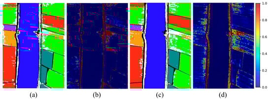
Figure 13. Open-set classification results and predictive uncertainty on the WHU-Hi-LongKou dataset. (a,b) BDL-$G^2$. (c,d) Proposed method.

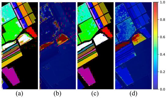
Figure 14. Open-set classification results and predictive uncertainty on the Salians dataset. (a,b) BDL-$G^2$. (c,d) Proposed method.

A similar trend is observed in the WHU-Hi-LongKou dataset. As shown in Figure 13, compared to the BDL-$G^2$ method, the proposed method demonstrates superior performance in uncertainty-aware unknown class identification. Specifically, the BDL-$G^2$ method often struggles to distinguish between known and unknown classes by predictive uncertainty. This limitation arises from the model’s insufficient capacity to capture the global distribution of known classes, leading to the omission of certain features. Consequently, these unrepresented features overlap with those of unknown class in the feature space, impairing the model’s ability to reliably differentiate between them. In contrast, the proposed method can more efficiently capture complex and nuanced data distributions through MCMC posterior inference, providing a valid uncertainty quantification for each sample. This allows a more accurate distinction between known and unknown classes.

Finally, we present the uncertainty quantification results on the Salinas dataset. As shown in Figure 14, both methods exhibit strong capability in identifying the unknown class. However, for the Grapes and Vinyard-U classes, BDL-$G^2$ tends to overemphasize unknown class identification (i.e., adjusting the decision threshold to favor the detection of unknown class), which leads to the misclassification of known classes as unknown. This limitation arises from the model’s insufficient ability to accurately capture the underlying data distribution. In contrast, the proposed method demonstrates superior performance on the Salinas dataset, achieving a more precise separation between known and unknown classes.

5.3. Sensitivity Analysis of Key Parameters

In the proposed GDAN model, the patch size, uncertainty threshold $ϵ$, and sampling number will potentially influence the performance of open-set HSI classification. To evaluate the effects of these parameters, additional experiments were conducted to analyze the parametric sensitivity of the GDAN.

(1) Patch size. In the open-set HSI classification task, the patch size directly influences the model’s ability to extract spectral spatial features. To evaluate the effect of patch size on open-set HSI classification, accuracy comparisons were conducted across five different patch sizes (1 × 1, 3 × 3, 5 × 5, 7 × 7, and 9 × 9) on three datasets in the 100-sample scenario, and the results are shown in Figure 15. In general, patch-based open-set HSI classification methods outperform the pixel-based method, which is mainly because the relationship between adjacent pixels can provide richer context information. Specifically, as the patch size increases from 1 × 1 to 5 × 5, the model’s performance generally improves across different datasets, reflecting the benefit of incorporating local contextual information. For instance, on the Pavia dataset, the $OA$ increases from 87.2% with 1 × 1 patches to 90.8% with 5 × 5 patches. Similarly, for the WHU-Hi-LongKou and Salinas datasets, the $OA$ improves from 88.1% to 92.1%, and from 87.6% to 90.4%, respectively. However, further enlarging the patch size leads to performance degradation for most HSI datasets, which may be explained by a larger patch size introducing redundant or irrelevant background information that impairs classification accuracy. Therefore, 5 × 5 was adopted as the optimal configuration.

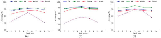
Figure 15. Effect of different patch sizes on open-set HSI classification. (a) Pavia dataset. (b) WHU-Hi-LongKou dataset. (c) Salians dataset.

(2) Uncertainty threshold. The uncertainty threshold $ϵ$ determines the decision boundary for separating known-class predictions from potential unknown samples. To assess its impact, we conduct a series of experiments by varying $ϵ$ and evaluating the model’s performance in terms of correctly identifying unknown instances while maintaining accurate classification of known classes, as shown in Figure 16. The results show that the choice of threshold significantly affects the trade-off: a lower threshold increases the identification of unknown samples but may reduce accuracy on known classes, while a higher threshold improves known-class classification at the cost of missing some unknown samples. These results confirm the importance of selecting an appropriate uncertainty threshold and demonstrate that our proposed method can achieve a balanced performance with a properly chosen value.

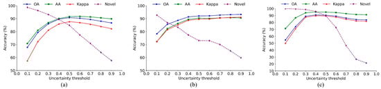
Figure 16. Sensitivity analysis of uncertainty threshold in open-set HSI classification. (a) Pavia dataset. (b) WHU-Hi-LongKou dataset. (c) Salians dataset.

(3) Sampling number. The sampling number $\left|n_s\right|$ is a critical factor in the proposed method and must be set carefully. The sensitivity of $OA$, $AA$, $Kappa$ and unknown accuracy to variations in sampling number under different sample proportions is illustrated in Figure 17. The sampling number $\left|n_s\right|$ was varied from 2 to 20 with an interval of 2. The first two rows show results for the Pavia, WHU-Hi-LongKou, and Salinas datasets under different sample proportions, respectively. Overall, model performance gradually improves with an increasing number of sampling iterations. This improvement is primarily attributed to the model’s capability to better capture the underlying data distribution with more samples, thereby mitigating the challenges associated with open-set classification that arise from insufficient sampling. Specifically, when the sampling number is limited, although the model can effectively classify known classes, the insufficient exploration of distribution patterns of complex multimodal data within the class leads to confusion between the features of known and unknown classes, preventing the model from accurately distinguishing unknown classes. As the sampling number increases, the model can estimate a more accurate sample probability distribution, thus achieving more accurate quantification of uncertainty and uncertainty-aware unknown class identification. Furthermore, as shown in the figure, when the number of sampling iterations reaches a certain number, the model’s performance in open-set classification stabilizes, fluctuating within a defined range. However, increasing the sampling number will also lead to higher computational costs. To effectively balance computational resource consumption with model performance, the number of sampling iterations was set to 10, ensuring efficiency without sacrificing accuracy.

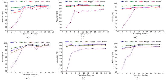
Figure 17. Model performance in open-set HSI classification under different sampling numbers. (a) Pavia dataset (T = 100). (b) WHU-Hi-LongKou dataset (T = 100). (c) Salians dataset (T = 100). (d) Pavia dataset (T = 200). (e) WHU-Hi-LongKou dataset (T = 200). (f) Salians dataset (T = 200).

5.4. Model Size and Computational Cost Analysis

Assessing the model’s size and computational cost is essential to understand its practical efficiency and resource requirements. Therefore, we selected two lightweight methods (MixerSENet and SSLR) and the BNN-based method (BDL-$G^2$), and reported a comparison of our method with these methods in terms of model size and computational efficiency, using the Salinas dataset as an example. For each method, the number of trainable parameters (Params), floating point operations (FLOPs), and inference time (Runtime) are reported, as shown in Table 10. The results show that BNN-based frameworks generally incur higher computational costs, as reflected in larger FLOPs, with the BDL-$G^2$ method and our proposed method having FLOPs of $204.17\times {10}^6$ and $\mathrm{22,202}\times {10}^6$, respectively. The relatively larger FLOPs and parameter count of our method mainly result from the incorporation of multimodal distribution modeling module, which is essential for capturing complex spectral–spatial variations and enabling reliable open-set decision boundaries. This design introduces additional computational overhead because it enhances feature expressiveness and facilitates more accurate separation between known and unknown classes in a high-dimensional feature space.

Table 10. Parameters, FLOPs, and inference time of different methods.

Method	Params	$\mathbf{FLOPs} (\times {10}^6$)	Runtime (s)
MixerSENet	53,146	7.894	15.7
SSLR	278,670	25.81	50.3
BDL-$G^2$	53,469	204.17	39.6
Ours	29,545,764	22,202	42.4

In future work, we will investigate lightweight and parameter-efficient multimodal distribution modeling mechanisms, and model compression strategies to reduce computational complexity while preserving the model’s ability to characterize multimodal distributions.

5.5. Limitations

The proposed GDAN integrates GANs with MCMC to explore the latent multimodal structure of the feature space, thereby enhancing the model’s ability to distinguish unknown samples. However, this advantage comes at the cost of increased computational overhead. Specifically, the multimodal distribution modeling module requires multiple rounds of MCMC sampling in the feature space and repeated forward passes to achieve stable mode exploration, resulting in a higher inference cost compared with conventional models. Thus, computational efficiency remains one of the primary limitations of the current approach. In addition, to mitigate potential performance degradation caused by class imbalance in the training data, this paper adopts a class-balanced sampling strategy. While effective in controlled settings, this assumption may not hold in real-world scenarios involving numerous minority classes or highly skewed class distributions. In such cases, the strategy may reduce data utilization efficiency and, to some extent, limit the model’s adaptability to complex environments. Consequently, improving computational efficiency and enabling robust multimodal prior construction under imbalanced data conditions represent promising directions for future research.

6. Conclusions

In this study, a novel global distribution-aware network is proposed for open-set HSI classification, which leverages trustworthy uncertainty modeling to facilitate the discovery of unknown classes in open-set environments. First, the introduction of the MCMC optimizes the model’s parameter space, enabling it to better capture the intra-class distribution diversity and thereby enhancing its ability to represent the global data distribution. Second, the use of GAN enables the generation of latent representations for potential unknown classes, improving the model’s capability to identify previously unseen objects. Finally, the introduction of the improved uncertainty quantification module provides an intuitive and effective indicator for the accurate identification of unknown class. Extensive experiments and analysis demonstrate that the proposed method can significantly improve open-set HSI classification performance compared with current state-of-the-art methods.

In the future, we will focus on the few-shot based open-set HSI classification, exploring how to effectively model complex posterior distributions with limited samples, further reducing the dependency of the model on labeled data.

References

- Chang, C.-I. Hyperspectral Data Exploitation: Theory and Applications; John Wiley & Sons: Hoboken, NJ, USA, 2007. [Google Scholar]
- Plaza, A.; Benediktsson, J.A.; Boardman, J.W.; Brazile, J.; Bruzzone, L.; Camps-Valls, G.; Chanussot, J.; Fauvel, M.; Gamba, P.; Gualtieri, A. Recent advances in techniques for hyperspectral image processing. Remote Sens. Environ. 2009, 113, S110–S122. [Google Scholar] [CrossRef]
- Bishop, C.A.; Liu, J.G.; Mason, P.J. Hyperspectral remote sensing for mineral exploration in Pulang, Yunnan Province, China. Int. J. Remote Sens. 2011, 32, 2409–2426. [Google Scholar] [CrossRef]
- Peyghambari, S.; Zhang, Y. Hyperspectral remote sensing in lithological mapping, mineral exploration, and environmental geology: An updated review. J. Appl. Remote Sens. 2021, 15, 031501. [Google Scholar] [CrossRef]
- Saleem, Z.; Khan, M.H.; Ahmad, M.; Sohaib, A.; Ayaz, H.; Mazzara, M. Prediction of microbial spoilage and shelf-life of bakery products through hyperspectral imaging. IEEE Access 2020, 8, 176986–176996. [Google Scholar] [CrossRef]
- Khan, M.H.; Saleem, Z.; Ahmad, M.; Sohaib, A.; Ayaz, H.; Mazzara, M. Hyperspectral imaging for color adulteration detection in red chili. Appl. Sci. 2020, 10, 5955. [Google Scholar] [CrossRef]
- Paoletti, M.E.; Haut, J.M.; Plaza, J.; Plaza, A. A new deep convolutional neural network for fast hyperspectral image classification. ISPRS J. Photogramm. Remote Sens. 2018, 145, 120–147. [Google Scholar] [CrossRef]
- Okwuashi, O.; Ndehedehe, C.E. Deep support vector machine for hyperspectral image classification. Pattern Recognit. 2020, 103, 107298. [Google Scholar] [CrossRef]
- Melgani, F.; Bruzzone, L. Classification of hyperspectral remote sensing images with support vector machines. IEEE Trans. Geosci. Remote Sens. 2004, 42, 1778–1790. [Google Scholar] [CrossRef]
- Li, J.; Bioucas-Dias, J.M.; Plaza, A. Semisupervised hyperspectral image segmentation using multinomial logistic regression with active learning. IEEE Trans. Geosci. Remote Sens. 2010, 48, 4085–4098. [Google Scholar] [CrossRef]
- Huang, H.; Shi, G.; He, H.; Duan, Y.; Luo, F. Dimensionality reduction of hyperspectral imagery based on spatial–spectral manifold learning. IEEE Trans. Cybern. 2019, 50, 2604–2616. [Google Scholar] [CrossRef]
- Beirami, B.A.; Mokhtarzade, M. Band grouping SuperPCA for feature extraction and extended morphological profile production from hyperspectral images. IEEE Geosci. Remote Sens. Lett. 2020, 17, 1953–1957. [Google Scholar] [CrossRef]
- Wang, J.; Chang, C.-I. Independent component analysis-based dimensionality reduction with applications in hyperspectral image analysis. IEEE Trans. Geosci. Remote Sens. 2006, 44, 1586–1600. [Google Scholar] [CrossRef]
- Camps-Valls, G.; Tuia, D.; Bruzzone, L.; Benediktsson, J.A. Advances in hyperspectral image classification: Earth monitoring with statistical learning methods. IEEE Signal Process. Mag. 2013, 31, 45–54. [Google Scholar] [CrossRef]
- Peng, J.; Sun, W.; Du, Q. Self-paced joint sparse representation for the classification of hyperspectral images. IEEE Trans. Geosci. Remote Sens. 2018, 57, 1183–1194. [Google Scholar] [CrossRef]
- Yuan, H.; Tang, Y.Y. Sparse representation based on set-to-set distance for hyperspectral image classification. IEEE J. Sel. Top. Appl. Earth Obs. Remote Sens. 2015, 8, 2464–2472. [Google Scholar] [CrossRef]
- Liu, J.; Wu, Z.; Wei, Z.; Xiao, L.; Sun, L. Spatial-spectral kernel sparse representation for hyperspectral image classification. IEEE J. Sel. Top. Appl. Earth Obs. Remote Sens. 2013, 6, 2462–2471. [Google Scholar] [CrossRef]
- Tang, Y.Y.; Lu, Y.; Yuan, H. Hyperspectral image classification based on three-dimensional scattering wavelet transform. IEEE Trans. Geosci. Remote Sens. 2014, 53, 2467–2480. [Google Scholar] [CrossRef]
- Liu, H.; Li, W.; Xia, X.-G.; Zhang, M.; Gao, C.-Z.; Tao, R. Central attention network for hyperspectral imagery classification. IEEE Trans. Neural Netw. Learn. Syst. 2022, 34, 8989–9003. [Google Scholar] [CrossRef]
- Hong, D.; Gao, L.; Yao, J.; Zhang, B.; Plaza, A.; Chanussot, J. Graph convolutional networks for hyperspectral image classification. IEEE Trans. Geosci. Remote Sens. 2020, 59, 5966–5978. [Google Scholar] [CrossRef]
- Chen, Y.; Jiang, H.; Li, C.; Jia, X.; Ghamisi, P. Deep feature extraction and classification of hyperspectral images based on convolutional neural networks. IEEE Trans. Geosci. Remote Sens. 2016, 54, 6232–6251. [Google Scholar] [CrossRef]
- Ge, Z.; Cao, G.; Li, X.; Fu, P. Hyperspectral image classification method based on 2D–3D CNN and multibranch feature fusion. IEEE J. Sel. Top. Appl. Earth Obs. Remote Sens. 2020, 13, 5776–5788. [Google Scholar] [CrossRef]
- Liang, H.; Bao, W.; Shen, X.; Zhang, X. Spectral–spatial attention feature extraction for hyperspectral image classification based on generative adversarial network. IEEE J. Sel. Top. Appl. Earth Obs. Remote Sens. 2021, 14, 10017–10032. [Google Scholar] [CrossRef]
- Huang, Y.; Peng, J.; Sun, W.; Chen, N.; Du, Q.; Ning, Y.; Su, H. Two-branch attention adversarial domain adaptation network for hyperspectral image classification. IEEE Trans. Geosci. Remote Sens. 2022, 60, 5540813. [Google Scholar] [CrossRef]
- Yang, X.; Cao, W.; Lu, Y.; Zhou, Y. Hyperspectral image transformer classification networks. IEEE Trans. Geosci. Remote Sens. 2022, 60, 5528715. [Google Scholar] [CrossRef]
- Xie, Z.; Hu, J.; Kang, X.; Duan, P.; Li, S. Multilayer global spectral–spatial attention network for wetland hyperspectral image classification. IEEE Trans. Geosci. Remote Sens. 2021, 60, 5518913. [Google Scholar] [CrossRef]
- Zhao, Z.; Xu, X.; Li, S.; Plaza, A. Hyperspectral image classification using groupwise separable convolutional vision transformer network. IEEE Trans. Geosci. Remote Sens. 2024, 62, 5511817. [Google Scholar] [CrossRef]
- Peng, Y.; Zhang, Y.; Tu, B.; Li, Q.; Li, W. Spatial–spectral transformer with cross-attention for hyperspectral image classification. IEEE Trans. Geosci. Remote Sens. 2022, 60, 5537415. [Google Scholar] [CrossRef]
- Liu, Y.; Hou, J.; Peng, Y.; Jiang, T. Distance-based hyperspectral open-set classification of deep neural networks. Remote Sens. Lett. 2021, 12, 636–644. [Google Scholar] [CrossRef]
- Du, Y.; Li, X.; Shi, L.; Li, F.; Xu, T. A prototype network for hyperspectral image open-set classification based on feature invariance and weighted Pearson distance measurement. IEEE Trans. Geosci. Remote Sens. 2024, 62, 5506917. [Google Scholar] [CrossRef]
- Chen, M.; Feng, S.; Zhao, C.; Qu, B.; Su, N.; Li, W.; Tao, R. Fractional Fourier-based frequency-spatial–spectral prototype network for agricultural hyperspectral image open-set classification. IEEE Trans. Geosci. Remote Sens. 2024, 62, 5514014. [Google Scholar] [CrossRef]
- Xu, H.; Chen, W.; Tan, C.; Ning, H.; Sun, H.; Xie, W. Orientational clustering learning for open-set hyperspectral image classification. IEEE Geosci. Remote Sens. Lett. 2024, 21, 5508605. [Google Scholar] [CrossRef]
- Feng, S.; Wang, S.; Xu, C.; Zhao, C.; Li, W.; Tao, R. Fractional Domain Information Enhanced Hyperspherical Prototype Learning Method for Hyperspectral Image Open-Set Classification. IEEE Trans. Geosci. Remote Sens. 2025, 63, 5515117. [Google Scholar] [CrossRef]
- Yue, J.; Fang, L.; He, M. Spectral-spatial latent reconstruction for open-set hyperspectral image classification. IEEE Trans. Image Process. 2022, 31, 5227–5241. [Google Scholar] [CrossRef]
- Liu, S.; Shi, Q.; Zhang, L. Few-shot hyperspectral image classification with unknown classes using multitask deep learning. IEEE Trans. Geosci. Remote Sens. 2020, 59, 5085–5102. [Google Scholar] [CrossRef]
- Ma, L.; Yang, Y.; Wang, G.; Li, Z.; Sun, W.; Du, Q. Open Set Domain Adaptation for Hyperspectral Image Classification Based on Reconstruction Discrepancy and Feature Alignment. IEEE J. Sel. Top. Appl. Earth Obs. Remote Sens. 2025, 18, 24829–24847. [Google Scholar] [CrossRef]
- Ji, F.; Zhao, W.; Wang, Q.; Emery, W.J.; Peng, R.; Man, Y.; Wang, G.; Jia, K. Spectral-spatial evidential learning network for open-set hyperspectral image classification. IEEE Trans. Geosci. Remote Sens. 2024, 62, 5503617. [Google Scholar] [CrossRef]
- Xie, Z.; Duan, P.; Liu, W.; Kang, X. Uncertainty-Aware Prototype Learning for Open-Set Hyperspectral Image Classification. In Proceedings of the 2024 2nd International Conference on Pattern Recognition, Machine Vision and Intelligent Algorithms (PRMVIA), Changsha, China, 24–27 May 2024; pp. 145–148. [Google Scholar]
- Xie, Z.; Duan, P.; Liu, W.; Kang, X.; Wei, X.; Li, S. Feature consistency-based prototype network for open-set hyperspectral image classification. IEEE Trans. Neural Netw. Learn. Syst. 2023, 35, 9286–9296. [Google Scholar] [CrossRef] [PubMed]
- Xi, B.; Zhang, W.; Li, J.; Song, R.; Li, Y. HyperTaFOR: Task-Adaptive Few-Shot Open-Set Recognition With Spatial-Spectral Selective Transformer for Hyperspectral Imagery. IEEE Trans. Image Process. 2025, 34, 4148–4160. [Google Scholar] [CrossRef]
- Pal, D.; Bose, S.; Banerjee, B.; Jeppu, Y. Morgan: Meta-learning-based few-shot open-set recognition via generative adversarial network. In Proceedings of the IEEE/CVF Winter Conference on Applications of Computer Vision, Waikoloa, HI, USA, 3–7 January 2023; pp. 6295–6304. [Google Scholar]
- Kong, S.; Ramanan, D. Opengan: Open-set recognition via open data generation. In Proceedings of the IEEE/CVF International Conference on Computer Vision, Montreal, QC, Canada, 10–17 October 2021; pp. 813–822. [Google Scholar]
- Pal, D.; Bundele, V.; Sharma, R.; Banerjee, B.; Jeppu, Y. Few-shot open-set recognition of hyperspectral images with outlier calibration network. In Proceedings of the IEEE/CVF Winter Conference on Applications of Computer Vision, Waikoloa, HI, USA, 3–8 January 2022; pp. 3801–3810. [Google Scholar]
- Haut, J.M.; Paoletti, M.E.; Plaza, J.; Li, J.; Plaza, A. Active learning with convolutional neural networks for hyperspectral image classification using a new Bayesian approach. IEEE Trans. Geosci. Remote Sens. 2018, 56, 6440–6461. [Google Scholar] [CrossRef]
- Preston, J.; Basener, W. Modeling Uncertainty in Hyperspectral Image Classification Using Neural Networks with Bayesian Monte Carlo Dropout. In Proceedings of the 2023 13th Workshop on Hyperspectral Imaging and Signal Processing: Evolution in Remote Sensing (WHISPERS), Athens, Greece, 31 October–2 November 2023; pp. 1–6. [Google Scholar]
- Chen, T.; Fox, E.; Guestrin, C. Stochastic gradient hamiltonian monte carlo. In Proceedings of the International Conference on Machine Learning, Beijing, China, 21–26 June 2014; pp. 1683–1691. [Google Scholar]
- Zhong, Y.; Hu, X.; Luo, C.; Wang, X.; Zhao, J.; Zhang, L. WHU-Hi: UAV-borne hyperspectral with high spatial resolution (H2) benchmark datasets and classifier for precise crop identification based on deep convolutional neural network with CRF. Remote Sens. Environ. 2020, 250, 112012. [Google Scholar] [CrossRef]
- Sun, Y.; Liu, B.; Wang, R.; Zhang, P.; Dai, M. Spectral–spatial MLP-like network with reciprocal points learning for open-set hyperspectral image classification. IEEE Trans. Geosci. Remote Sens. 2023, 61, 5513218. [Google Scholar] [CrossRef]
- He, X.; Chen, Y.; Huang, L. Bayesian deep learning for hyperspectral image classification with low uncertainty. IEEE Trans. Geosci. Remote Sens. 2023, 61, 5506916. [Google Scholar] [CrossRef]
- Liu, Q.; Yue, J.; Fang, Y.; Xia, S.; Fang, L. HyperMamba: A Spectral-Spatial Adaptive Mamba for Hyperspectral Image Classification. IEEE Trans. Geosci. Remote Sens. 2024, 62, 1–14. [Google Scholar] [CrossRef]
- Alkhatib, M.Q.; Roy, S.K.; Jamali, A. MixerSENet: A Lightweight Framework for Efficient Hyperspectral Image Classification. IEEE Geosci. Remote Sens. Lett. 2025, 22, 5509805. [Google Scholar] [CrossRef]
Disclaimer/Publisher’s Note: The statements, opinions and data contained in all publications are solely those of the individual author(s) and contributor(s) and not of MDPI and/or the editor(s). MDPI and/or the editor(s) disclaim responsibility for any injury to people or property resulting from any ideas, methods, instructions or products referred to in the content. |
© 2025 by the authors. Licensee MDPI, Basel, Switzerland. This article is an open access article distributed under the terms and conditions of the Creative Commons Attribution (CC BY) license (https://creativecommons.org/licenses/by/4.0/).