Integrating Satellite and Field Data for Glacier Melt Modeling in High-Mountain Asia: A Case Study on Passu Glacier

Highlights

What are the main findings?

• A simplified melt model accurately estimated bare ice melt on Passu Glacier (error = 0.48 m w.e., 9%).
• Satellite-derived albedo variability significantly influenced melt estimates.
• Elevation was the dominant topographic factor controlling ice melt, exceeding the influence of slope or aspect.

What is the implication of the main finding?

• The melt model is reliable and scalable for estimating bare ice melt in remote, data-scarce regions.
• Using multi-date satellite imagery for albedo improves the accuracy of ice melt simulations.
• The approach supports effective glacier monitoring in the Karakoram with minimal field data.

Abstract

Glaciers in High-Mountain Asia, the so-called “Third Pole,” are critical water sources but remain poorly monitored due to rugged topography and limited accessibility. We present an integrated approach that combines remote sensing with ground-based observations to model ice melt of the Passu Glacier (Pakistan) from 5 August to 13 October 2023. Meteorological data from two automatic weather stations and ablation measurements from four stakes were used together with satellite-derived albedo (Landsat 8 OLI), surface temperature (Landsat 9 TIRS), and topography (ALOS AW3D30 DSM) to implement an enhanced T-index melt model accounting for net shortwave and longwave radiation. Model performance was evaluated against station and satellite data and ablation stake measurements using leave-one-out cross-validation. The estimated total ice melt volume was 16 million m³ w.e. during the monitoring period, with an average melt of 3.60 m w.e. The model reproduced observed stake ablation with an uncertainty of 0.48 m w.e. (9% of average measured melt). Elevation was identified as the dominant melt driver (β = −0.501, unique R² = 0.199), with aspect and slope exerting secondary influences through their effect on solar radiation and shading. Our findings demonstrate that combining minimal but strategically located field data with satellite products provides a physically consistent and scalable framework for glacier melt estimation in data-scarce regions of the Third Pole, with relevance for hydrological monitoring and climate adaptation.

1. Introduction

The high-mountain regions of Asia, collectively known as the Third Pole, host the largest concentration of glaciers outside the polar areas. With over 100,000 glaciers and a critical role in supplying meltwater to some of the world’s most densely populated river basins, this region is a key component of both regional and global hydrological systems [1,2]. However, this cryospheric reservoir is increasingly threatened by climate change. Rising air temperatures, altered precipitation regimes, and feedback from surface processes are altering the mass balance of glaciers, with far-reaching consequences for water availability, ecosystem functioning, and natural hazard risk [3,4].

Within this context, the Karakoram Range stands out as a complex and atypical sector of the Third Pole. Unlike much of the Himalayan arc, where glaciers are retreating rapidly, the Karakoram displays a more heterogeneous response, including stable or advancing glaciers, known in the literature as the “Karakoram anomaly” [5,6]. Glaciers here are located at very high altitudes, often above 3500 m a.s.l., and are frequently affected by debris cover, which complicates both the energy balance and melt dynamics [7,8,9]. In addition, the occurrence of glacier surge-type behavior contributes further variability and uncertainty to assessments of glacier mass changes [10].

Despite their scientific significance, glaciers in the Karakoram remain under-monitored, primarily due to the region’s extreme topography, remoteness, and limited accessibility. Field-based glaciological measurements are scarce and spatially constrained, making it difficult to acquire continuous or representative datasets [11,12]. This limitation reflects a broader challenge for cryospheric research across High-Mountain Asia.

Given these constraints, remote sensing has become an indispensable tool for observing glaciers in inaccessible regions. Satellite data allow for the estimation of surface elevation change, glacier extent, velocity fields, surface temperature, and albedo over large spatial domains. However, estimates of glacier melt derived solely from remote sensing still carry substantial uncertainty, especially in debris-covered areas and regions with complex topography or where energy balance modeling is not constrained by ground-based data [13]. There is therefore a clear need for integrated approaches that combine satellite observations with targeted field measurements.

Several types of melt models have been developed [12,14,15,16,17], and they are mainly based on two different approaches: physical energy-balance models and empirical temperature-index models [15]. The former may be defined as a model in which each of the relevant energy fluxes at the glacier surface is computed from physically based calculations considering the necessary meteorological variables, and the melt rate is calculated from the sum of the radiative and energy fluxes. The latter may be defined as a model in which the melt rate is calculated from an empirical formula in which air temperature is the sole considered input variable, although additional input variables, such as incoming shortwave radiation, may be incorporated through parameterizations based on time and location. These models explicitly include net shortwave radiation and surface albedo as additional predictors of melt [15,18]. Other studies have incorporated net longwave radiation, demonstrating that a simplified yet physically consistent formulation can reproduce ice melt at an AWS site when all radiative components are accounted for [16]. In parallel, physically based energy and mass balance models have recently been applied to debris-covered glaciers in the Karakoram, such as Batura, to quantify how supraglacial debris modifies surface energy fluxes and long-term mass balance over the past two decades [19]. In this context, temperature-index models have been widely used for both glaciological and hydrological applications due to their parsimony in data requirement in comparison with the more sophisticated energy-balance models [15].

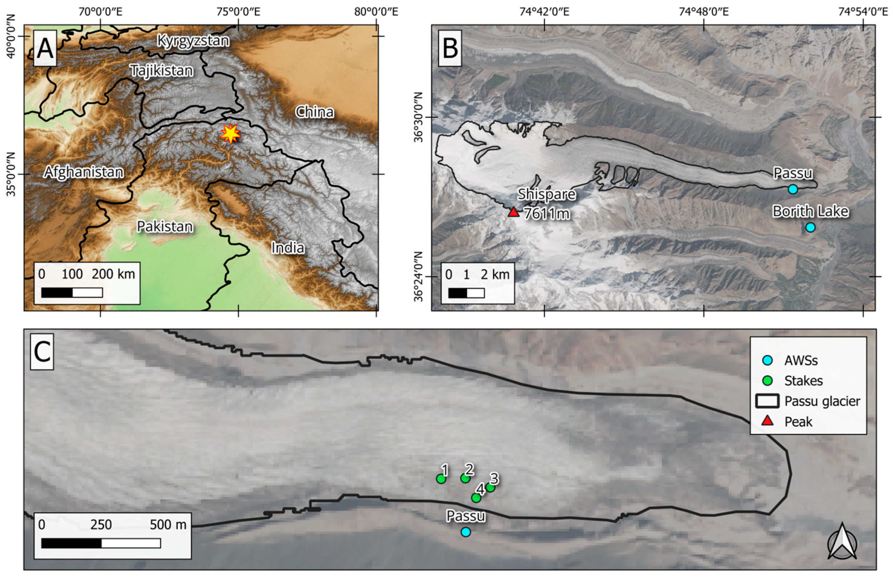
In this regard, applications of enhanced T-index models that combine net shortwave and net longwave radiation with both remote sensing products and in situ measurements remain scarce in Pakistan region. This study adopts such an integrated framework, focusing on Passu Glacier, located in the Hunza Valley of the Karakoram (Figure 1). We combined high-resolution satellite imagery with in situ meteorological and glaciological observations to develop and validate a physically based ice melt model that is both accurate and scalable. Due to the extreme logistical challenges of accessing high-altitude glaciers across the Third Pole, our approach aims to validate a scalable methodology that can be applied to other glaciers in similar contexts, characterized by high elevation, limited accessibility, and debris-free surface conditions. Although temporally limited (5 August to 13 October 2023), our field data provide critical constraints for the calibration and verification of remote sensing-based ice melt estimates. Unlike previous studies in the Karakoram that relied on simplified T-index models or constant albedo assumptions (e.g., [12]), this work integrates multi-date satellite-derived albedo and longwave radiation into a physically consistent melt model, validated with in situ data.

By integrating complementary datasets, our aim is to provide a transferable methodology that can be applied to other glaciers in the Third Pole region. Since the importance of understanding this region’s cryosphere is critical, beyond its methodological scope, this study contributes to a broader scientific and societal imperative.

Study Area

Passu Glacier is located in the Hunza Valley, within the Karakoram Range. Compared to other large glaciers in the valley, Passu is relatively debris-free, covering an area of 53.47 km² [20]. It extends for about 38 km in length [20] from east to west, flanked by the Gulkhin and Batura Glaciers [21], with an elevation range from 2686 to 7638 m a.s.l.

At the terminus of the glacier lies Passu lake, a moraine-dammed glacial lake. Although the lake drains naturally, it has experienced at least two outburst flood events in the last two decades, which caused significant damage, including the destruction of a bridge along the Karakoram Highway (KKH) and several houses in the Passu village on the right bank of the Hunza River [21,22]. The recurrence interval of such outburst events appears to be irregular, with frequencies ranging from 2 to 5 years [22].

Regarding glacier changes, previous studies have documented limited glacier terminus retreat [21,23,24]. Additionally, Passu Glacier has been the focus of research on black carbon deposition [25] and the hydrochemistry of its meltwater [26], indicating its importance as a case study for understanding cryospheric and hydrological processes in the region.

2. Data and Methods

This study combines satellite remote sensing data with sparse but valuable ground-based observations to model surface ice melt over the Passu Glacier.

We first describe the available field data, including both meteorological and glaciological observations. This is followed by a detailed overview of the remote sensing data used. The final part of this section outlines the modeling framework adopted to estimate the key input variables, as well as the structure of the ice melt model itself.

All variables were assessed for distributional characteristics using histograms, a Q-Q plot, and the Shapiro–Wilk test for normality. A significance level of α = 0.05 was adopted for all normality tests, and the associated p-values (p) are reported. If the null hypothesis of normality was not rejected (p ≥ 0.05), variables are described as mean ± standard deviation (sd); otherwise, they are presented as median values with inter-quartile range (IQR).

2.1. Ground-Based Data

2.1.1. Meteorological Observations

Meteorological data were collected from two permanent automatic weather stations (AWSs) installed in August and September 2022 (Figure 1). The first station (Passu AWS) is located on the lateral moraine of the Passu Glacier (36.455°N, 74.856°E; 2945 m a.s.l.). The second (Borith Lake AWS) is situated near Borith Lake (36.431°N, 74.867°E; 2680 m a.s.l.), approximately 3.5 km from the Passu AWS. Both stations were installed within the framework of the “Glaciers & Students” project, an international initiative implemented by the United Nation Development Program (UNDP) to promote scientific and social development in Pakistan.

The Passu AWS is equipped with a compact, all-in-one sensor by LSI Lastem, capable of measuring air temperature, relative humidity, atmospheric pressure, wind speed and direction, and incoming solar radiation. However, it lacks instruments to measure longwave radiation (both incoming and outgoing) as well as reflected solar radiation. In contrast, Borith Lake AWS includes a complete set of sensors that conform to World Meteorological Organization (WMO) standards [27], including a net radiometer. This makes it suitable for validating modeled radiative fluxes and other meteorological variables used in this study.

Data from both stations were recorded at hourly intervals. A quality control (QC) procedure was applied to identify and remove nonsensical and erroneous values and assess the percentage of valid data retained for analysis.

2.1.2. Glaciological Observations

Ablation measurements were conducted during the summer 2023 field campaign by installing four bamboo stakes (each 12 m in length) with a steam drill in the ablation zone of the Passu Glacier on 5 August 2023 (Figure 1). Due to the challenging logistics and accessibility constraints of the Passu Glacier, the installation of only four ablation stakes was feasible. The four stakes were positioned along the central flowline of the ablation zone, spanning an elevation range of 2916–2932 m a.s.l., to capture the main melt gradient. Local slope and aspect are reported in

Table 1. Location (latitude and longitude) and description of local conditions (elevation, slope, and aspect) per ablation stake.

Ablation Stake	Latitude	Longitude	Elevation (m a.s.l.)	Slope	Aspect (Azimuth Angle)
1	36.457°N	74.855°E	2932	89.10°	165.47°
2	36.457°N	74.856°E	2926	89.10°	160.20°
3	36.457°N	74.857°E	2917	89.10°	173.66°
4	36.456°N	74.856°E	2916	89.10°	173.05°

.

The emersions of the ablation stakes from the glacier surface were remeasured on 13 October 2023. The stake data provided point-scale observations of surface ice melt and played a dual role in this study. First, they were used for model calibration, serving as the empirical basis for estimating the parameters of the melt model. Second, they were used for model validation, enabling the assessment of model accuracy and performance.

AWS data from 2022 provided baseline meteorological forcing, while stake measurements (Aug–Oct 2023) were used for calibration and validation. Stake readings were taken at installation and removal dates; measurement uncertainty was estimated at ±0.05 m w.e.

2.2. Remote Sensing Data

To characterize glacier geometry and surface conditions, we used the updated perimeter of the Passu Glacier from the “New Pakistan Glacier Inventory” developed under the umbrella of the “Glaciers & Students” project [20].

In addition, a suite of satellite-derived products was employed to provide key input variables for the surface melt modeling framework:

• Digital Surface Model (DSM): AW3D30 (30 m resolution), derived from ALOS/PRISM data. This dataset was used for computing topographic parameters (i.e., slope, aspect, and shading) and for distributing air temperature and solar radiation.
• Landsat 8 OLI (30 m resolution) was used to derive glacier-wide surface albedo via narrowband-to-broadband conversion.
• Landsat 9 TIRS (100 m spatial resolution, resampled at 30 m) was used to validate outgoing longwave radiation estimates through surface kinetic temperature retrieval.
• To conduct the albedo analysis, we used Google Earth Engine (GEE), a cloud-based platform for image for preprocessing, cloud masking, and extraction of surface reflectance data for albedo computation.

The DSM used in this study (scene code ALPSMLC30_N036E074_DSM) was obtained from the Japanese Aerospace Exploration Agency (JAXA). AW3D30 is a global digital surface model derived from PRISM (Panchromatic Remote-sensing Instrument for Stereo Mapping), an optical sensor onboard the Advanced Land Observing Satellite (ALOS), which operated from 2006 to 2011. This DSM product offers a horizontal resolution of ~30 m and vertical accuracy better than 5 m, making it suitable for topographic correction and terrain-based modeling of radiative fluxes.

2.3. Modeling Framework

To simulate surface ice melt over the Passu Glacier, we implemented a physically based modeling framework that combines satellite-derived products with in situ meteorological observations. The model accounts for the main radiative components of the surface energy balance, including shortwave and longwave radiation fluxes. Ice melt rates were estimated using an enhanced temperature-index approach, in which turbulent heat fluxes (sensible and latent) are not explicitly modeled but are instead implicitly incorporated into empirical melt factors that depend on air temperature. This approach maintains physical realism while reducing data requirements, making it suitable for remote high-mountain environments.

The modeling system is designed to spatially and temporally distribute key energy balance variables across the whole glacier surface, integrating topographic effects (i.e., elevation, slope, aspect, and shading) and atmospheric conditions (i.e., temperature, humidity, and cloud cover). This allows for realistic estimation of spatially distributed ice melt, even in the absence of direct surface energy measurements.

In the following sections, we detail the procedures used to derive each ice melt model component across the whole glacier surface, including incoming and outgoing shortwave radiation, incoming and outgoing longwave radiation, and air temperature. We also explain the implementation of the enhanced T-index melt model, and how calibration and validation were performed using field-based ablation data.

2.3.1. Air Temperature (T_A-point)

Air temperature across the whole glacier surface (T_A-point) was reconstructed by applying the mean tropospheric lapse rate of –6.5 °C/km [28]. This lapse rate was applied to daily mean air temperature values recorded at the Passu AWS, in order to correct for elevation differences across the glacier. The correction was implemented at the spatial resolution of the AW3D30 DSM, generating a distributed daily air temperature field over the glacier surface. This approach allows for the incorporation of topographic variability in temperature modeling, which is essential for accurately estimating melt in high-altitude, complex terrains.

Although the model was run for the full hydrological year, in this study we report T_A results only for the period between 5 August and 13 October 2023, corresponding to the availability of ablation measurements for calibration and validation.

2.3.2. Incoming Shortwave Radiation (SW_in-point)

Incoming solar radiation (SW_in-point) over the whole Passu Glacier was modeled following the multi-step approach reported by [29], which progressively increases in physical complexity. The methodology involves four sequential steps: (i) flat exo-atmospheric surface, assuming no topography, (ii) sloped exo-atmospheric surface (SW_in-exo-point), incorporating slope and aspect effects, (iii) sloped surface with orographic complexity (i.e., accounting for topographic shading) (SW_{in-exo-shade-point}), and (iv) actual atmosphere and surface conditions (SW_in-point) integrating atmospheric transmissivity and using data acquired by the Passu AWS (SW_in-Passu).

This modeling framework incorporates several key parameters: slope (S_point), aspect (A_point), solar declination (δ_point), sunrise/sunset hour angles (w_sr-point/w_ss-point), and atmospheric transmissivity (τ_A). The effects of terrain-induced shading were calculated using the AW3D30 DSM, applying the approach by [30].

The radiation for a sloped surface under exo-atmospheric conditions was estimated using the following formulation:

$$\begin{array}{ll}{SW}_{in-exo-point}=& I\times E\times k\\ & \times [\left(\sin {\delta }_{point}\times \sin {\mathsf{\Phi }}_{point}\times \cos S_{point}\right)\\ & \times \left(w_{ss-point}-w_{sr-point}\right)\\ & -\left(\sin {\delta }_{point}\times \cos {\mathsf{\Phi }}_{point}\times \cos S_{point}\times \cos A_{point}\right)\\ & \times \left(w_{ss-point}-w_{sr-point}\right)\\ & +\left(\cos {\delta }_{point}\times \cos {\mathsf{\Phi }}_{point} \times \cos S_{point}\right)\times \left(\sin w_{ss}-\sin w_{sr}\right)\\ & +\left(\cos {\delta }_{point}\times \sin {\mathsf{\Phi }}_{point}\times \sin S_{point}\times \cos A_{point}\right)\\ & \times \left(\sin w_{ss-point}-\sin w_{sr-point}\right)\\ & -\left(\cos {\delta }_{point}\times \sin A_{point}\times \sin S_{point}\right)\\ & \times \left(\cos w_{ss-point}-\cos w_{sr-point}\right)]\end{array}$$

(1)

where I is the average solar irradiance at the mean Earth–Sun distance (1367 W m⁻²), E is the eccentricity factor accounting for Earth’s elliptical orbit [31], k is a unit conversion factor to MJ day⁻¹, and Φ_point is the latitude. w_sr-point and w_ss-point have opposite values because of the hour. The slope S_point ranges from 0° (i.e., horizontal) to 90° (i.e., vertical) [32]. The aspect is related to the south; thus, 0° represents south, 90° east, −90° west, and ±180° north [32].

The calculation of w_sr-point and w_ss-point for sloped surfaces followed the analytical approach by [30], which also accounts for auto-shading. In particular, steep north-facing slopes in the Northern Hemisphere may remain shaded for part or all of the day.

The last step involved computing SW_in-point, which distributes incoming solar radiation over the glacier surface by integrating shading conditions (derived from mountain peak–grid cell elevation differences [29]) and cloudiness. The latter was taken into account by estimating τ_A:

$${\tau }_A={\displaystyle \frac{{SW}_{in-Passu}}{{SW}_{in-exo-Passu}}}$$

(2)

where SW_in-exo-Passu is the sloped exo-atmospheric incoming solar radiation, estimated for the pixel of the Passu AWS. The atmospheric transmissivity generally ranges from nearly 0 to slightly higher than 1 [33]. Values higher than 1 are due to multireflection, caused by the presence of fresh snow over the surroundings.

Finally, five combinations of shading and atmospheric conditions were identified following the scheme proposed by [17], depending on whether the Passu AWS and/or each grid point were shaded and whether the sky was clear or cloudy. Based on all these combinations, SW_in-point was calculated as

$${SW}_{in-point}={SW}_{in-exo-point}\times {\tau }_A$$

(3)

The modeling framework provides incoming shortwave radiation at hourly resolution for each glacier grid cell. To ensure consistency with the temporal scale of other variables and the melt model, hourly SW_in values were aggregated into daily means prior to integration into the ice melt calculation.

Although the model was run for the full hydrological year, in this study we report SW_in results only for the period between 5 August and 13 October 2023, corresponding to the availability of ablation measurements for calibration and validation. We described each variable and how it was considered during the calculations in

Table 2. Description of each variable used for calculation of SW_in. For each variable it is reported whether it is considered constant, modeled, or measured.

Symbol	Parameter	Assessment Method
I	Average solar irradiance	Constant
E	Eccentricity factor	Modeled, temporally variable
k	Unit conversion factor	Constant
δpoint	Solar declination	Modeled, temporally and spatially variable
Φpoint	Latitude	Derived from DSM
Spoint	Slope	Modeled from DSM
wsr-point/wss-point	Sunrise/sunset hour angles	Modeled, temporally and spatially variable
Apoint	Aspect	Modeled from DSM
τA	Atmospheric transmissivity	Modeled, temporally variable
SWin-exo-point	Sloped exo-atmospheric incoming solar radiation at each pixel	Modeled, temporally and spatially variable
SWin-exo-shade-point	Sloped exo-atmospheric incoming solar radiation, considering shading conditions at each pixel	Modeled, temporally and spatially variable
SWin-point	Incoming solar radiation at each pixel	Modeled, temporally and spatially variable
SWin-exo-Passu	Sloped exo-atmospheric incoming solar radiation at Passu AWS pixel	Modeled, temporally variable
SWin-Passu	Incoming solar radiation at Passu AWS	Measured

.

2.3.3. Surface Albedo (α_point)

Outgoing solar radiation (SW_out) is governed by the reflection of incoming solar radiation at the surface and is directly related to albedo (α, defined as the fraction of incident solar irradiance that is reflected by the surface [34]). As the Passu AWS is not equipped with a net radiometer, surface albedo was derived from satellite imagery.

We estimated broadband albedo across the whole glacier surface using surface reflectance data from Landsat 8 OLI, processed via the Google Earth Engine (GEE) platform. After applying a cloud mask based on the CFMASK algorithm, we used the narrowband-to-broadband conversion algorithm proposed by Liang [35]:

$$\begin{gathered} {\mathsf{\alpha }}_{point}=0.356{\mathsf{\alpha }}_{2-point}+0.130{\mathsf{\alpha }}_{4-point}+0.373{\mathsf{\alpha }}_{5-point}+0.085{\mathsf{\alpha }}_{6-point} \\ +0.072{\mathsf{\alpha }}_{7-point}-0.0018 \end{gathered}$$

(4)

where α_i-point (i = 2, 4, 5, …) represents narrowband albedo derived from the i-th L8/OLI band for each pixel. This formula has been widely validated in previous glaciological studies [36,37].

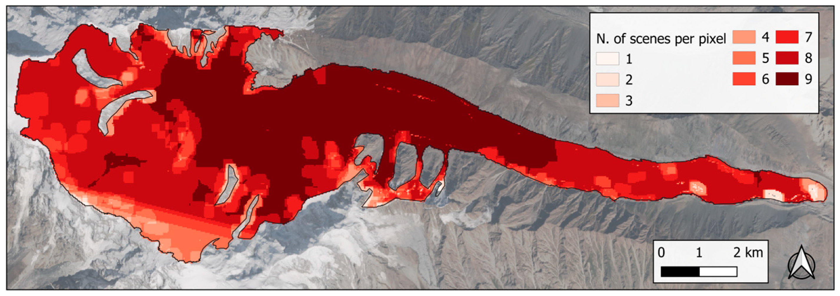
To ensure reliable surface coverage, only scenes with more than 70% valid pixels within the glacier perimeter were retained, resulting in a total of nine usable scenes (

Table 3. Code scene, acquisition date, and glacier coverage percentage of Landsat 8 OLI images.

Code Scene	Acquisition Date	Glacier Coverage (%)
LC81500342023221LGN00	09 Aug 2023	85
LC81500352023221LGN00	09 Aug 2023	89
LC81500342023253LGN00	10 Sept 2023	88
LC81500352023253LGN00	10 Sept 2023	90
LC81490352023262LGN00	19 Sept 2023	90
LC81500342023269LGN00	26 Sept 2023	50
LC81490352023278LGN00	05 Oct 2023	98
LC81500342023285LGN00	12 Oct 2023	97
LC81500352023285LGN00	12 Oct 2023	94

and Figure 2). Due to temporal gaps, which result in an insufficient temporal coverage of the studied period, and partial cloud cover, which prevents us from obtaining complete spatial coverage of the glacier for each acquisition, albedo was treated as time-invariant but spatially distributed.

For each pixel, the mean value across all valid dates within the ablation monitoring period (5 August–13 October 2023) was used to represent the surface albedo, minimizing the effect of possible outliers.

2.3.4. Incoming Longwave Radiation (LW_in)

Daily mean incoming longwave radiation (LW_in) was estimated using air temperature and cloudiness derived from the Passu AWS dataset, following the approach reported by [29,38]. To estimate cloudiness, we computed cloud transmissivity (τ) by comparing measured incoming shortwave radiation (SW_in) with clear-sky values (SW_in-CS), modeled using a truncated Fourier series fitted to the whole 2023 dataset:

$$\begin{array}{ll}{SW}_{in-CS}=245.5& -116.9\times \cos \left({\displaystyle \frac{day\times 2\pi }{365}}\right)\\ & +46.4\\ & \times \sin \left({\displaystyle \frac{day\times 2\pi }{365}}\right)\\ & -9.7\times \cos \left(2{\displaystyle \frac{day\times 2\pi }{365}}\right)-12.2\times \sin \left(2{\displaystyle \frac{day\times 2\pi }{365}}\right)\end{array}$$

(5)

where day is the Julian day of the year.

The atmospheric emissivity (ε) was then calculated as a function of cloudiness (n), combining clear-sky (ε_CS) and fully cloudy (ε_CL) conditions. The latter was assumed to be nearly constant and close to 1 [39]. ε_CS was derived following the method by Konzelmann et al. [40]. Atmospheric emissivity was computed using

$$\epsilon ={\epsilon }_{CS}\times \left(1-n^2\right)+{\epsilon }_{CL}\times n^2$$

(6)

Finally, LW_in was calculated by applying the Stefan–Boltzmann law:

$${LW}_{in}=\epsilon \times \sigma \times {\left(T_A+273.15\right)}^4$$

(7)

where σ is the Stefan–Boltzmann constant (5.67 × 10⁻⁸ W m⁻² K⁻⁴), and T_A is the air temperature from the Passu AWS.

This methodology builds on the physical understanding that under clear-sky conditions, incoming longwave radiation primarily depends on the vertical profiles of temperature and humidity in the lower atmosphere, with approximately 80% of the radiation originating from the lowest 500 m and more than 50% from the lowest 100 m above the surface [41]. As a result, LW_in is often estimated from surface observations by assuming standard atmospheric profiles for temperature and humidity [42,43,44,45]. This approach is particularly suited for high-mountain regions where detailed vertical atmospheric profiles are rarely available and AWS data are often limited to surface-level measurements.

Given its atmospheric origin, LW_in was assumed to be spatially uniform across the whole glacier surface, consistent with assumptions adopted in other previous glaciological modeling studies [17,29]. Although LW_in was modeled over the entire year, in this study we present results only for the period between 5 August and 13 October 2023, corresponding to the availability of ablation stake measurements.

2.3.5. Outgoing Longwave Radiation (LW_out-point)

Daily mean outgoing longwave radiation (LW_out-point) was modeled over the whole glacier surface using the Stefan–Boltzmann law, based on the glacier surface temperature (T_S-point):

$${LW}_{out-point}={\epsilon }_S\times \sigma \times {\left(T_{S-point}+273.15\right)}^4$$

(8)

where ε_S is the ice emissivity assumed to be equal to 1 [38]. As direct measurements of surface temperature were unavailable, T_S-point was estimated from the distributed air temperature field (T_A-point) (see Section 2.3.1), using the empirical relationship developed by Oerlemans [38], which assumes that the glacier surface temperature is in equilibrium with the air temperature only when the latter is below the melting point. Accordingly, surface temperature was constrained so that it did not exceed 0 °C:

$$T_{s-point}=min\left(T_{A-point},0\right)$$

(9)

This means that the surface temperature was spatially and temporally distributed, being derived for each grid cell and for each day of the full hydrological year, using the elevation-corrected air temperature field. This approach allows us to incorporate topographic and temporal variability in the estimation of LW_out over the entire glacier surface.

Although the model was run for the full hydrological year, in this study we report LW_out results only for the period between 5 August and 13 October 2023, corresponding to the availability of ablation measurements for calibration and validation.

2.3.6. Ice Melt Modeling (M_point)

Ice melt on glacier surfaces occurs when three main conditions are met: the surface temperature reaches 0 °C, the surface energy budget is positive, and albedo is lower than 0.40 [28]. To simulate ice melt, we applied the methodology developed and tested by Senese et al. [16], which builds upon the enhanced T-index formulation by Pellicciotti et al. [15]. This new model improves the standard T-index approach by explicitly incorporating net longwave radiation (LW_net-point) into the energy–melt relationship while simplifying the treatment of turbulent heat fluxes, which are included implicitly via the empirical coefficient. The model estimates ice melt at each glacier grid point using the following conditional equation:

$$\begin{array}{c} \\ M_{point}=\left\{\begin{array}{c}TMF\times T_{A-point}+SLMF\times \left[\left(1-{\alpha }_{point}\right)\times {SW}_{in-point}+{LW}_{net-point}\right], T_{S-point}=0 °\mathrm{C} and {\alpha }_{point}<0.40\\ 0, T_{S-point}<0 °\mathrm{C} and {\alpha }_{point}\ge 0.40\end{array}\right.\end{array}$$

(10)

where TMF is the temperature melting factor (0.031 m w.e. °C⁻¹ day⁻¹), SLMF is the radiative melting factor (−0.003 m w.e. (W m⁻²)⁻¹ day⁻¹), and LW_net-point is the difference between LW_in and LW_out-point. The two melting factors were assessed using the data of ice ablation measured at the 4 selected sites simultaneously by regression model. Melting factors estimated from field data were taken as constant in time and space [33].

This formulation allows us to maintain the physical contributions of radiative fluxes (both shortwave and longwave) while encapsulating the more complex turbulent fluxes into temperature-dependent terms. The choice of thresholds (T_S-point = 0 °C and α_point < 0.40) ensures that melt is computed only under physically plausible surface conditions.

The model was applied at the grid-cell level, allowing the simulation of spatially distributed ice melt across the whole Passu Glacier for the period 5 August–13 October 2023.

2.3.7. Model Validation

To assess the accuracy of the modeled variables and the resulting ice melt estimates, we applied a multi-faceted validation approach using independent datasets and established statistical metrics (

Table 4. Distribution and validation methods for each modeled parameter.

Parameter	Distribution	Input Data	Method	Data for Validation	Reference
TA-point	Spatial and temporal	Passu AWS	Elevation gradient	Borith AWS	Senese et al. (2014) [28]
SWin-point	Spatial and temporal	Passu AWS	Astronomical, geographical and geometrical parameters	Borith AWS	Senese et al. (2016) [29]
αpoint	Spatial only	Satellite (Landsat)	Empirical method	Borith AWS	Fugazza et al. (2016) [46]
LWin	Temporal only	Passu AWS	Empirical method	Borith AWS	Senese et al. (2016) [29]
LWout-point	Spatial and temporal	Passu AWS	Empirical method	Satellite (Landsat 9 TIRS)	Oerlemans (2000) [38]

).

The meteorological variables T_A-point, SW_in-point, α_point, and LW_in were validated against daily mean values recorded by Borith Lake AWS. Only days with complete hourly datasets were included in the validation. Model performance was evaluated using the following metrics: bias error (BE), mean absolute error (MAE), root mean square error (RMSE), bias-removed RMSE (BRRMSE), and R-Squared (R²). These metrics allow us to assess both the magnitude and direction of deviations between modeled and observed values.

To validate LW_out-point over the whole glacier surface, we used surface temperature retrieved from three Landsat 8/9 TIRS scenes (

Table 5. Code scene, acquisition date, and acquisition time of Landsat 8/9 TIRS images.

Code Scene	Acquisition Date	Acquisition Time
LC91490352023222LGN00	10 Aug 2023	05:35:10 UTC
LC91490352023254LGN00	11 Sept 2023	05:35:27 UTC
LC81490352023278LGN00	05 Oct 2023	05:35:30 UTC

). The scenes were averaged between them. Surface kinetic temperature was extracted from Band 10 (TIRS-1: 10.6–11.19 µm), which provides 100 m resolution thermal data. The surface reflectance product (Collection 2 Level 2) was used, which includes atmospheric correction and internal blackbody calibration. Using these satellite-derived temperatures (T_{Landsat-point}), we calculated LW_{out,val-point} via the Stefan–Boltzmann law to be used to validate LW_out-point:

$${LW}_{out,val-point}={\epsilon }_s·\sigma ·{\left(T_{Landsat-point}+273.15\right)}^4$$

(11)

Regarding ice melt, due to the limited number of ablation stakes (n = 4), it was not possible to split the dataset into two independent calibration and validation subsets. To address this limitation, we applied a leave-one-out cross-validation (LOOCV) procedure (i.e., a particular case of leave-p-out cross-validation with p = 1), which ensures that each data point is used once for validation while the remaining are used for calibration. This method avoids overfitting and allows us to compute robust error estimates for ice melt simulations.

3. Results

3.1. Meteorological Variables

3.1.1. Air Temperature

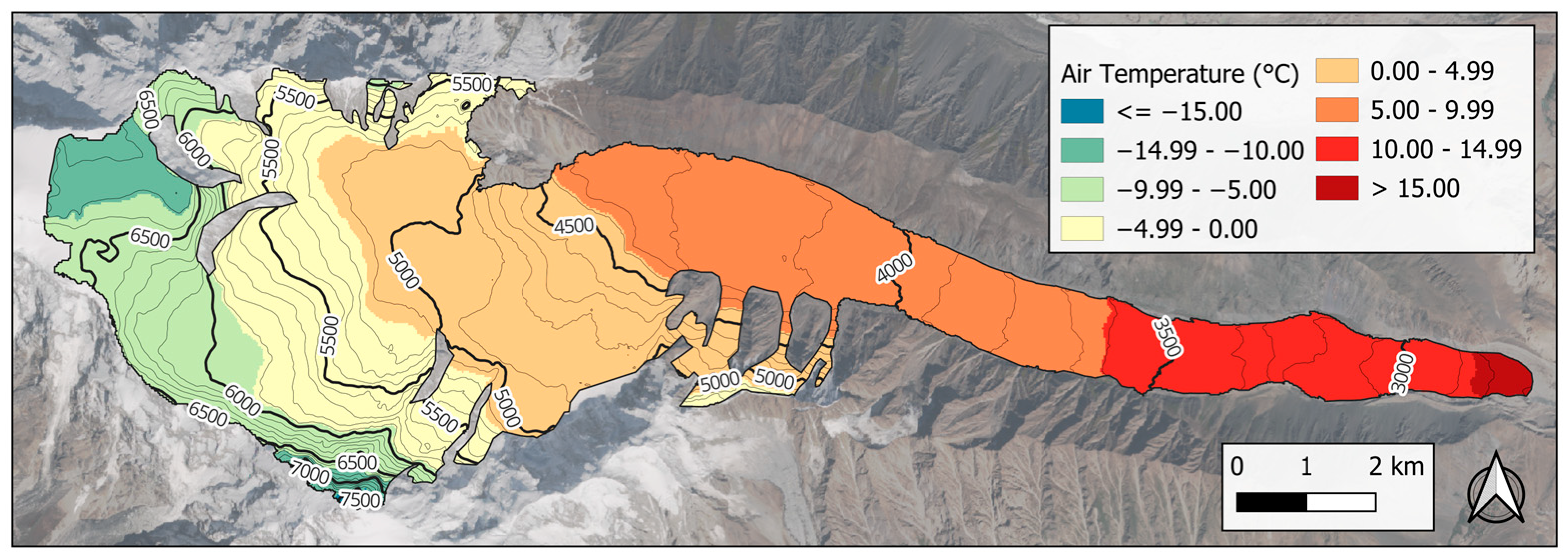
During the ablation stake monitoring period (5 August to 13 October 2023), the daily air temperature modeled over the entire Passu Glacier showed a clear asymmetric distribution (Figure 3). The overall median temperature was +1.49 °C with an interquartile range (IQR) of 7.59 °C. The lowest daily median occurred on 8 October 2023 with –8.02 °C (IQR = 10.10 °C), while the highest was on 21 August 2023 at +7.18 °C (IQR = 10.10 °C).

Considering the full spatial distribution across the glacier, the absolute minimum modeled air temperature was –25.13 °C (7638 m a.s.l., 8 October 2023), and the maximum was +22.26 °C (2686 m a.s.l., 21 August 2023).

At the Passu AWS, air temperature followed a similar pattern, with a gradual cooling trend from August to October. The daily minimum was +5.83 °C (8 October), and the maximum reached +20.50 °C (21 August), confirming consistency with the distributed values.

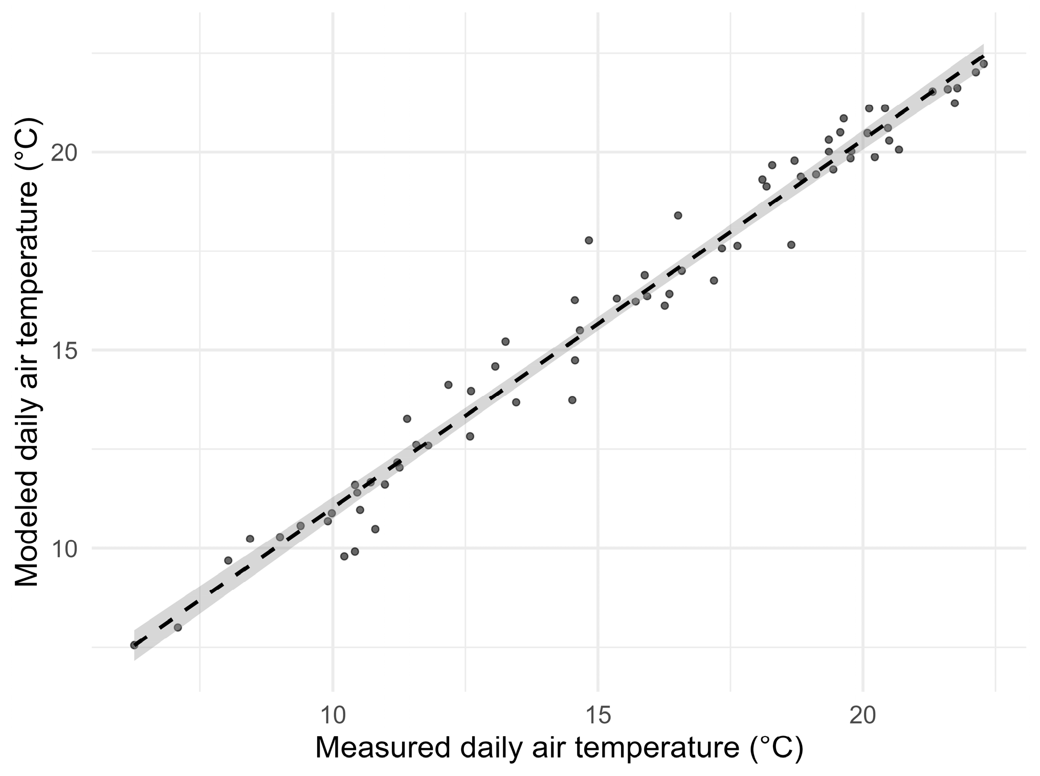
The approach for distributing air temperature was validated modeling air temperature at the Borith Lake AWS elevation using Passu AWS data. By comparing such modeled air temperatures with the measured one by Borith Lake AWS from 5 August to 13 October 2023, a BE of +0.63 °C, a MAE of +0.79 °C, an RMSE of +0.99 °C (corresponding to 6.4% of the mean value of all the daily values), a BRRMSE of +0.76 °C, and an R² of 0.97 were observed. These results show a good agreement between the measured and the modeled values (Figure 4).

3.1.2. Incoming Shortwave Radiation and Albedo

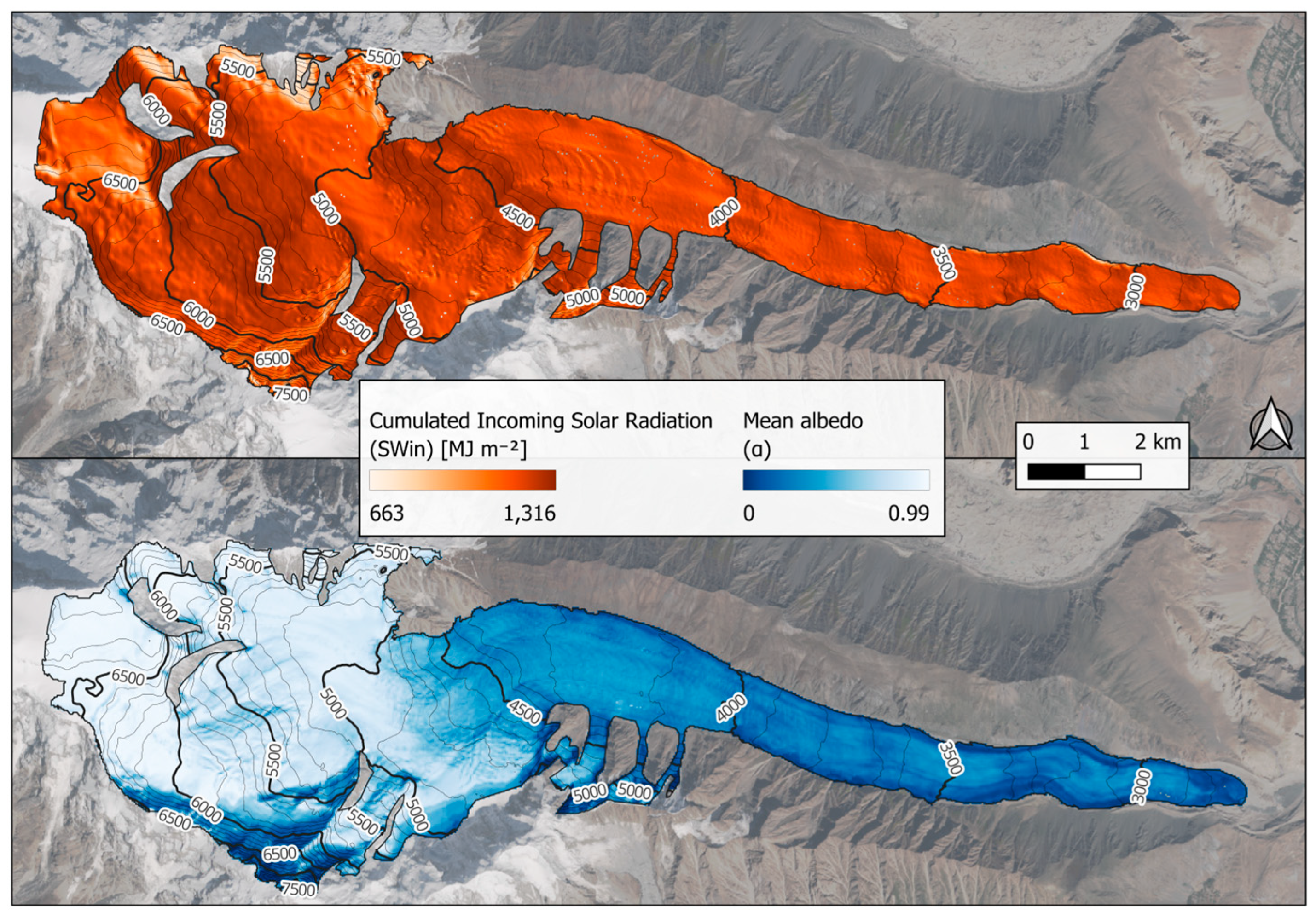
From 5 August to 13 October 2023, the modeled daily incoming shortwave radiation ranged between 57.90 W m⁻² (8 October) and 306.12 W m⁻² (9 August), with a median of 172.34 W m⁻² (IQR = 125.76 W m⁻²), over the entire glacier. Cumulative SW_in-point for the entire study period is illustrated in Figure 5 to better elucidate melt dynamics. The maximum value of cumulated incoming solar radiation is 1315.63 MJ m⁻² (6259 m a.s.l., slope = 44°, aspect = E), and the minimum value is 662.85 MJ m⁻² (5413 m a.s.l., slope = 69°, aspect = SW).

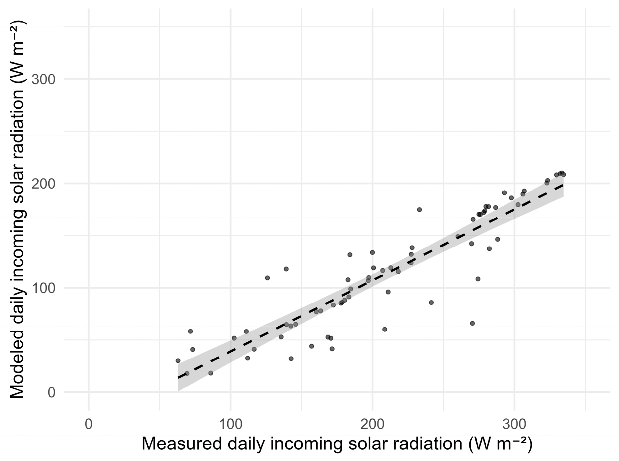
Model validation against Borith Lake AWS measurements yielded a BE of −96.54 W m⁻², a MAE of 96.54 W m⁻², an RMSE of 102.32 W m⁻², a BRRMSE of 33.92 W m⁻², and an R² of 0.81 (from 5 August to 13 October 2023). Despite slight underestimation, the overall performance is acceptable (Figure 6).

The median albedo over the glacier was 0.52, ranging from 0.01 to 0.99 (IQR = 0.58) (Figure 5). Albedo was found to increase with elevation: median albedo rises from around 0.14 at 2500–3000 m a.s.l. to 0.94 at 6500–7000 m a.s.l. Above 7000 m, a.s.l. albedo shows low medians (~ 0.08–0.10), likely due to local topographic shadowing.

To validate albedo estimates, we extracted the value for the Borith Lake AWS location, obtaining a mean of 0.09, which was compared to the measured mean albedo of 0.12 derived from Borith Lake AWS shortwave radiation data. The modeled albedo was slightly underestimated by 0.03. Albedo calculations were restricted to the central hours of days (10 am–3 pm LT) when the solar incidence angles are smaller, thus ensuring the greatest possible accuracy and reliability of the albedo calculations (following [47,48,49]). Since only a single mean value is available, it was not possible to compute statistical metrics as performed for the other parameters.

Using the modeled SW_in-point and satellite-derived α_point, we calculated cumulative net shortwave radiation over the glacier surface from 5 August to 13 October 2023. Values ranged from 141 MJ m⁻² to 14,506 MJ m⁻², with a median of 6863 MJ m⁻² (IQR = 7922 MJ m⁻²).

3.1.3. Incoming Longwave Radiation

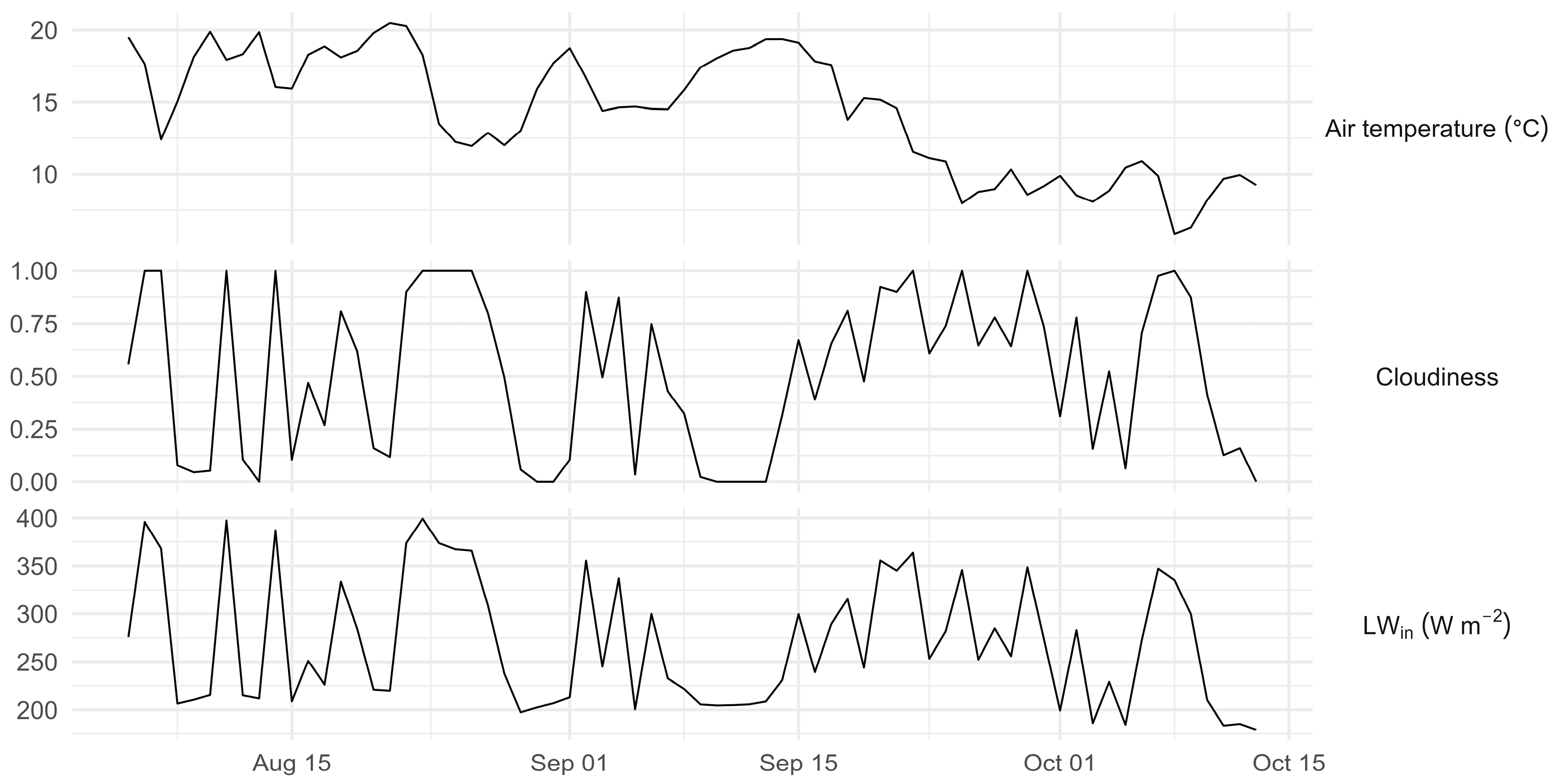
From 5 August to 13 October 2023, the temporal distribution of LW_in was non-normal, with a median of 251.72 W m⁻² and an IQR of 124.56 W m⁻². Daily minima and maxima ranged from 179.22 W m⁻² (13 October) to 399.22 W m⁻² (23 August) (Figure 7). LW_in variability reflected the influence of air temperature and cloudiness, with a bimodal cloudiness distribution: 33% of days had low cloudiness (< 0.2), and 30% had high cloudiness (> 0.8) (median cloudiness = 0.54; IQR = 0.76) [29].

Incoming longwave radiation was validated with the Borith Lake AWS data for the study period, showing a BE of −49.69 W m⁻², a MAE of 62.29 W m⁻², an RMSE of 72.61 W m⁻² (corresponding to 22.65% of the mean value of all daily values), a BRRMSE of 52.95 W m⁻², and an R² of 0.45. Although the model performance for incoming longwave radiation was almost satisfactory when compared to Borith Lake AWS data, part of the observed discrepancies can be attributed to known limitations in dome-type pyrgeometer measurements [50]. Solar heating of the instrument dome, especially under clear-sky and low-wind conditions, can cause overestimation of LW_in values by more than 10% according to previous studies [51,52]. Additional sources of uncertainty include frost formation and aerosol deposition on the dome surface, which can impair optical clarity and distort measurements. In general, instrument accuracy for LW_in measurements is estimated to be about 20 W m⁻² [45,53] or better under well-maintained and ventilated conditions [54,55]. These sources of error should be considered when interpreting the validation metrics.

3.1.4. Surface Temperature and Outgoing Longwave Radiation

From 5 August to 13 October 2023, daily mean surface temperature estimates showed a non-normal distribution, with a median value of 0 °C over the study period. Notably, 59.42% of the days had a median surface temperature equal to 0 °C. This is primarily due to the modeling approach, which constrains the surface temperature so that it remains at or below the melting point (Equation (7)). The minimum value is −25.13 °C (7638 a.s.l., on 8 October 2023), and the maximum value is 0.00 °C, due to definition (Equation (7)).

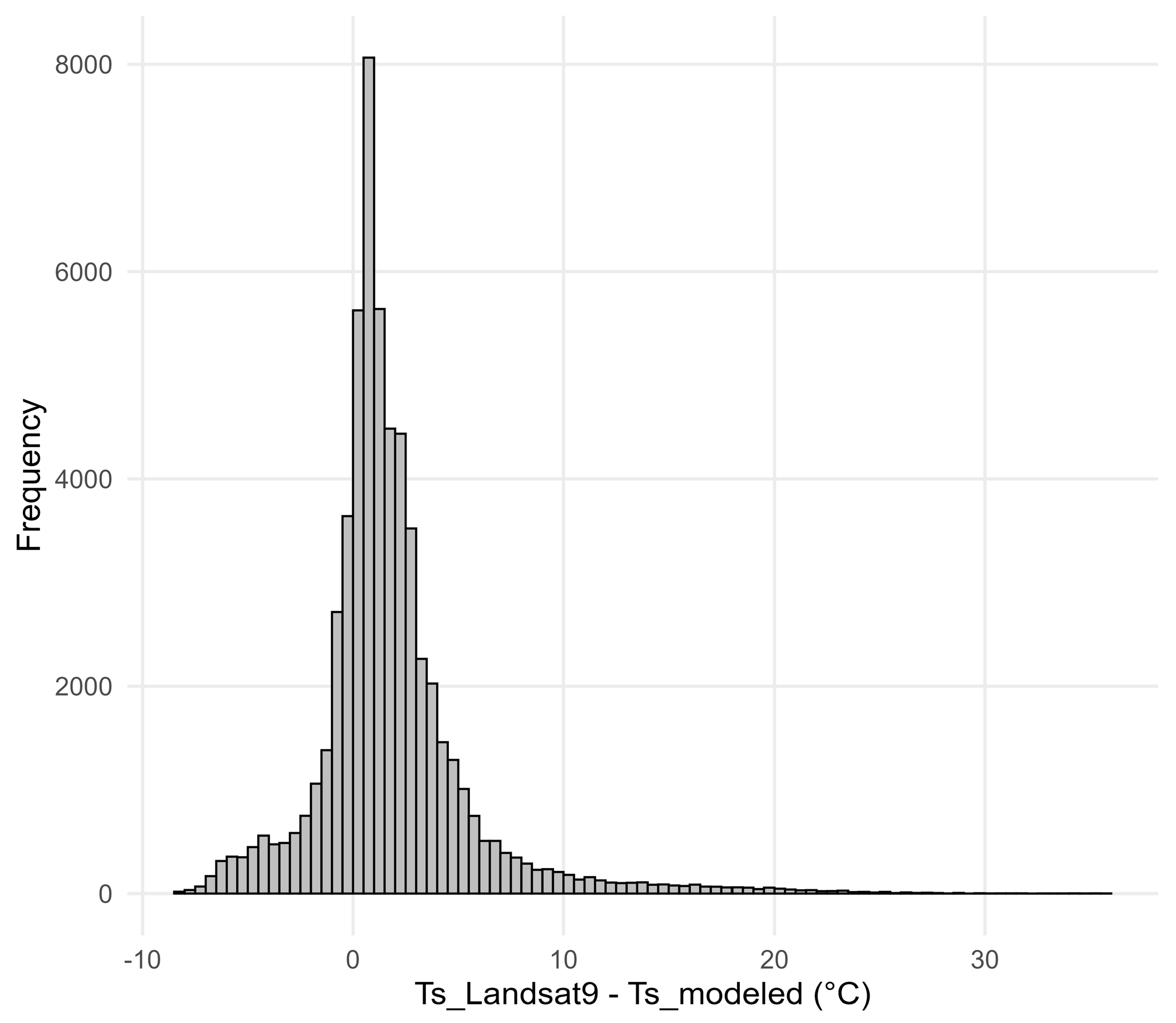
We validated these results with the averaged surface temperatures retrieved from the Landsat 9 satellite. We observed a BE of −1.83 °C, MAE of 2.69 °C, RMSE of 4.24 °C, a BRRMSE of 3.82 °C, and an R² of 0.57. Most residuals were between 0 and +1 °C, suggesting good model performance, despite a negative bias (Figure 8). The presence of a long-tailed positive distribution indicates that negative outliers contributed more to the error metrics.

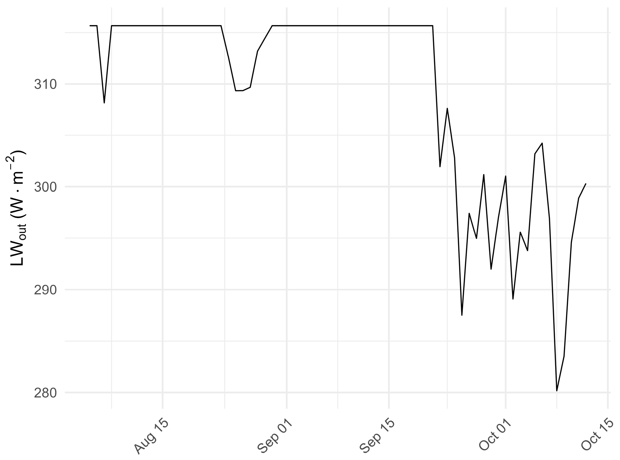
Modeled daily mean LW_out-point was also non-normally distributed, with a median value of 315.66 W m⁻² (IQR = 29.68 W m⁻²). The minimum daily median was 280.17 W m⁻² (IQR = 42.94 W m⁻², 8 October), and the maximum was 315.66 W m⁻² (IQR = 0 W m⁻², 5 August) (Figure 9).

To validate this parameter we used the LW_{out,val-point} derived from the averaged three Landsat 9 scenes compared to the modeled LW_out-point of the same day, which shows a BE of −2.67 W m⁻², a MAE of 13.16 W m⁻², an RMSE of 20.98 W m⁻² (corresponding to 6.7% of the average value of all the pixels), a BRRMSE of 20.81 W m⁻², and an R² of 0.48.

3.2. Ice Melt

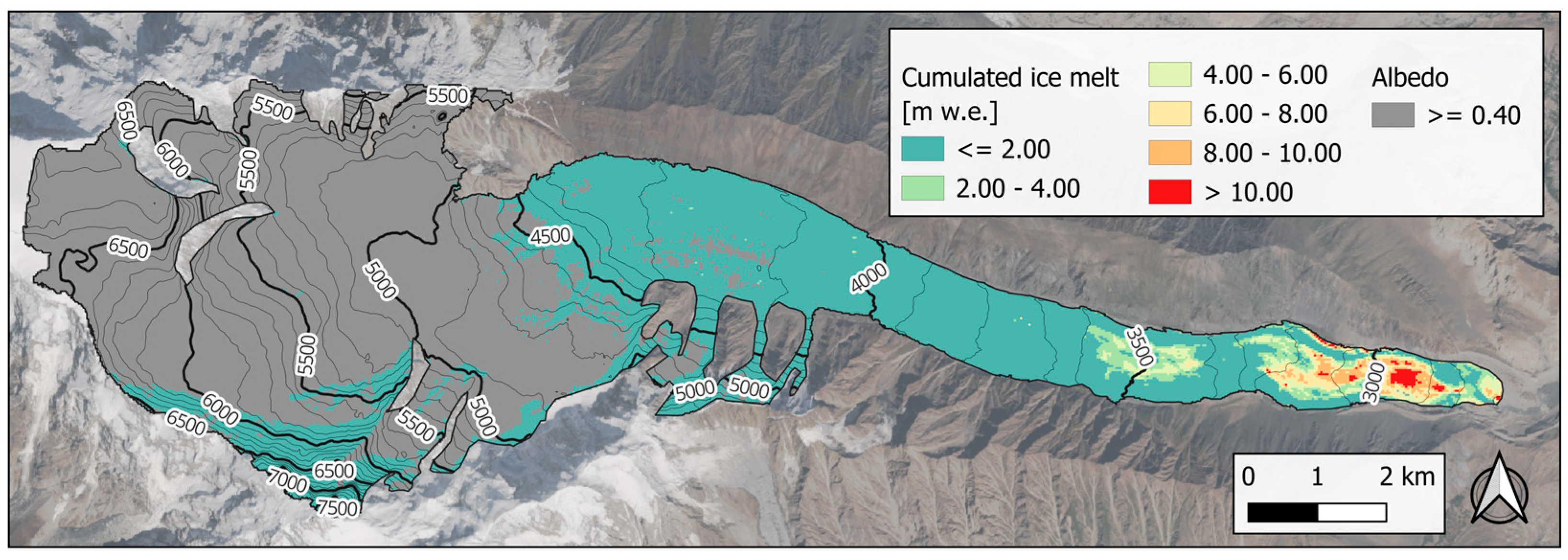
Over the study period (5 August to 13 October 2023), Passu Glacier lost a total of 16 million m³ w.e., corresponding to a mean ice loss of 4.22 m w.e. across the glacier bare ice surface.

The spatial distribution of melt is highly skewed, with a dominant peak at 0 m w.e., indicating that most of the glacier surface exhibited no melt during the study period, resulting in an overall median melt of 0 m w.e. (Figure 10). However, when considering only grid cells where melt occurred, the median melt rises to 3.60 m w.e. (IQR = 4.33 m w.e.), with a maximum of 14.11 m w.e.

Ablation measurements from four stakes on Passu Glacier provided observed melt values ranging from 4.55 to 6.91 m w.e. (

Table 6. Measured and modeled ice melt (m w.e.) at each ablation stake. The modeled values were calculated applying the LOOCV. The difference (∆M) between modeled and measured ice melt are also reported.

Stake	Measured Melt (m w.e.)	LOOCV Modeled Melt (m w.e.)	ΔM (m w.e.)
1	4.55	5.14	+0.60
2	5.28	4.60	−0.68
3	6.91	4.98	−1.93
4	5.13	5.21	+0.08

). By applying the LOOCV, the model successfully reproduced these observations, with an error of 0.48 m w.e. (estimated by dividing the standard deviation of the differences between modeled and measured ice melt by the square root of the number of the ablation stakes [28]), equivalent to approximately 9% of the average observed melt. This result indicates good model performance, particularly demonstrating the model’s ability to accurately replicate observed ablation patterns, especially in areas subject to intense melting.

4. Discussion

4.1. Factors Driving Ice Melt

To better understand the spatial variability of ice melt across Passu Glacier, we explored its relationship with topographic factors, namely elevation, slope, and aspect. Only pixels with positive cumulative melt were included in the analysis to isolate the drivers of actual ablation. To investigate which topographic factors most strongly influence cumulative ice melt, we applied a standardized multiple linear regression using four predictors: elevation, slope, and the south- and east-facing components of aspect. Aspect was decomposed into its cardinal components to avoid the circularity inherent in angular data. Two key metrics were used to assess the influence of each predictor: (i) the standardized regression coefficient (β) and (ii) the unique contribution to R² (

Table 7. Standardized regression results for cumulative melt. The table reports standardized coefficient (|β|), standard error (SE), t-statistic (t), p-value (p), unique R², and variance inflation factor (VIF).

Predictor	β	SE	t	p	Unique R2	VIF
Elevation	−0.501	0.016	−31.57	<2 × 10−16	0.199	1.262
Slope	−0.101	0.016	−6.455	1.3 × 10−10	0.008	1.236
Aspect south component	+0.164	0.016	+10.441	<2 × 10−16	0.022	1.231
Aspect east component	−0.025	0.016	−1.635	0.102	< 0.001	1.236

). In addition, we performed the following checks: (i) we analyzed the correlation matrix between the predictors (

Table 8. Correlation matrix of topographic predictors.

Predictor	Elevation	Slope	Aspect South Component	Aspect East Component
Elevation	1.000	−0.431	0.108	0.142
Slope	−0.431	1.000	0.026	−0.027
Aspect south component	0.108	0.026	1.000	0.426
Aspect east component	0.142	−0.027	0.426	1.000

), and (ii) we calculated the Variance Inflation Factor (VIF) for multicollinearity diagnostics (Table 7). Moreover, to minimize the potential influence of spatial autocorrelation among neighboring pixels (which could artificially inflate the strength of the statistical relationships), we tested the robustness of our results by repeating the analysis on a thinned dataset. Specifically, we selected one pixel every 300 m, thereby reducing the likelihood that adjacent pixels with similar characteristics would bias the regression outcomes (

Table 9. Model results for thinned sample (n = 111). The R² of the model is 0.319.

Predictor	β	Unique R2
Elevation	−0.340	0.222
Slope	−0.047	0.003
Aspect south component	0.045	0.003
Aspect east component	0.015	0.001

).

The results of the standardized multiple regression are reported in

Table 10. Model summary (full dataset). The table reports sample size (n), R², adjusted R² (R² adj), and residual standard error (RMSE).

n	R2	R2 adj	RMSE
3891	0.226	0.225	0.880

. These data highlight how elevation and the aspect south component dominate glacier melt. Indeed, holding other predictors constant, elevation shows a negative standardized coefficient (β = −0.501), consistent with decreasing ice melt at higher elevations due to the temperature lapse rate. South-facing exposure has a positive influence on the model (β = +0.164), consistently with the increased solar irradiance on south-facing slopes in the Northern Hemisphere. In contrast, slope exhibits a small but statistically significant negative effect (β = −0.101), which can be explained with the fact that steeper surfaces experience less favorable solar incidence and greater auto-shading probability. The aspect east component was found to be negligible as its p-value is greater than 0.05 (β = −0.025; p = 0.102). Unique R² values mirror these patterns (elevation: 0.199; slope: 0.008; aspect south component: 0.022, aspect east component: < 0.001). Analysis on multicollinearity between predictors highlights low values (all VIFs < 5), supporting coefficient stability. The analysis on the thinned sample confirmed the robustness of these findings, with elevation still explaining the majority of ice melt variability (elevation unique R² = 0.222) and only negligible differences in coefficients or model fit (R² = 0.319 vs. 0.227 in the full dataset).

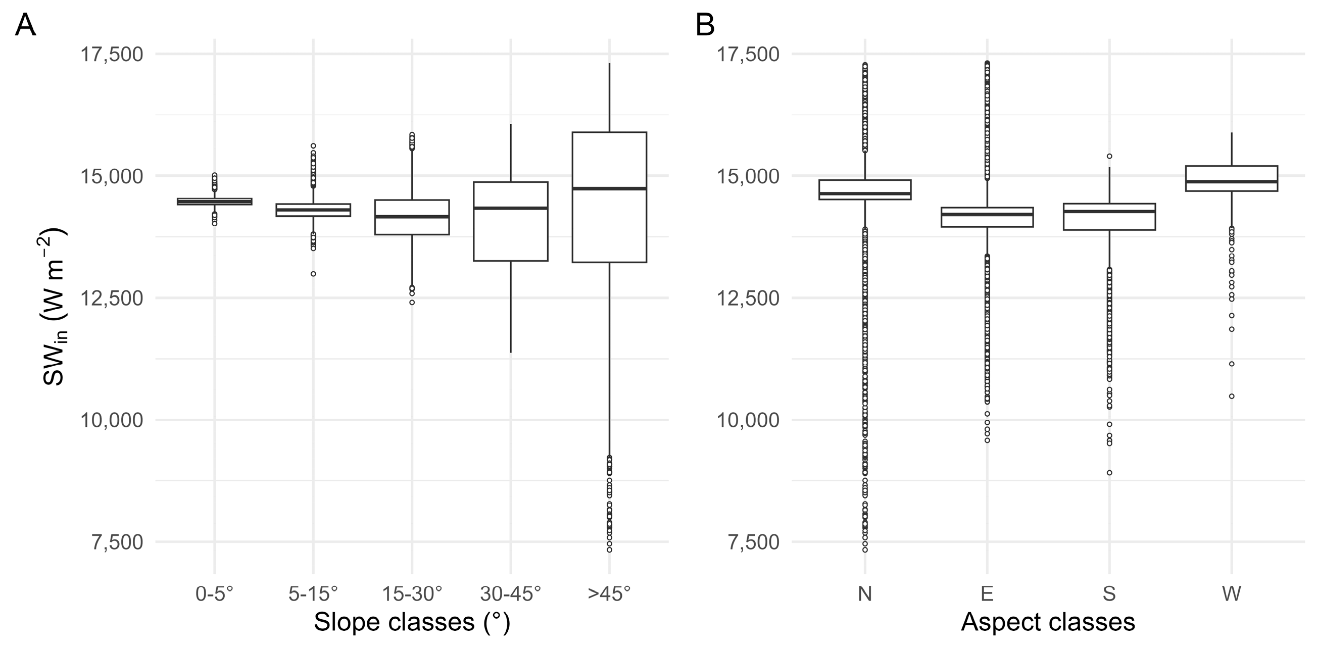
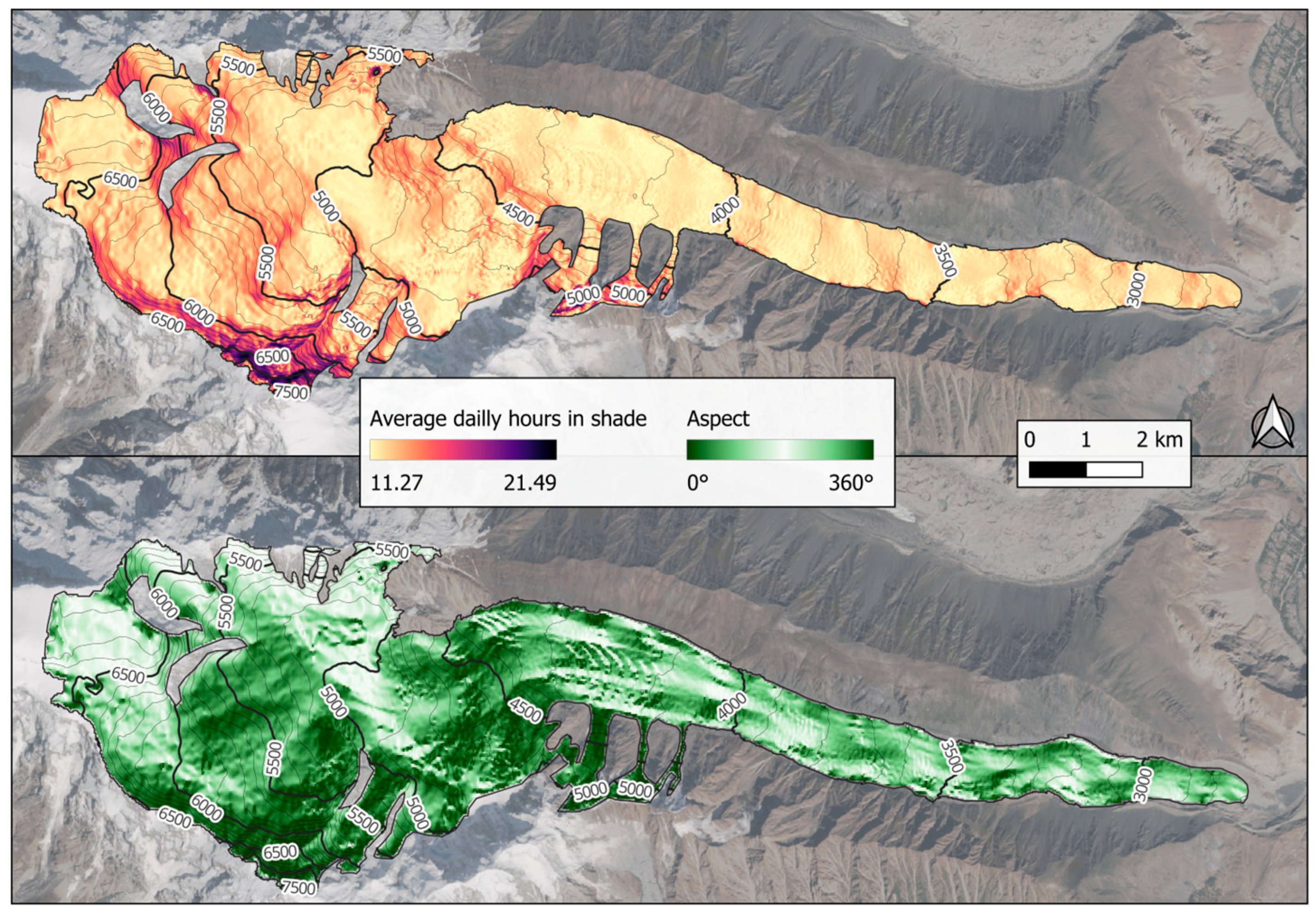
Since SW_in is the melt model component mainly depending on slope and aspect, we also performed the same analysis for the incoming solar radiation. The results show that while the median SW_in remains stable across slope classes, the spread (dispersion) of values increases with slope (Figure 11A), reflecting greater variability in solar irradiance due to shading and orientation effects. As regards aspect, no clear pattern is visible across the cardinal directions (Figure 11B), although lower SW_in values are more frequent on steep north-facing slopes, consistent with increased shading probability [30]. To support this, we also computed the average number of shaded hours per day for each pixel, confirming that north-facing pixels experience more shading (Figure 12).

4.2. Possible Uncertainties Related to Applied Approaches

In addition to the uncertainties of the input datasets, our modeling framework relies on different simplified assumptions that introduce additional sources of uncertainty in the simulated melt patterns.

The first source of uncertainty is represented by the approach used for distributing air temperature, which is assumed to vary only according to an elevation gradient. However, temperature gradients can differ over the glacier due to local topographic effects. This simplification could lead to errors in the distributed air temperature values used to drive the melt model.

As regards the incoming shortwave radiation models, we assume spatially constant cloudiness over the glacier. However, this parameter can vary spatially, introducing additional uncertainty in the estimated SW_in.

Assuming temporally constant albedo and emissivity = 1 introduces potential biases. While these assumptions simplify modeling in data-scarce contexts, future work should incorporate time-varying albedo and emissivity corrections. More precisely, surface albedo is assumed to be temporally constant even if spatially variable. In reality, albedo can change during the ice melt season because of snowfall events (which increase albedo), liquid precipitation (which can temporarily decrease ice albedo and induce brightening in the following days) [47], and the seasonal darkening phenomenon related to dust and impurity accumulation.

Moreover, incoming longwave radiation is treated as spatially constant over the glacier, although it is expected to vary with cloudiness and to be locally modified near the glacier margins by effect of the surrounding rocks. This simplification could underestimate the spatial variability of LW_in.

Outgoing longwave radiation is computed under the assumption that glacier surface temperature equals air temperature up to 0 °C. In glacierized terrain, surface temperature can deviate from air temperature; thus, this approximation could cause errors both in outgoing longwave radiation and in the identification of melt conditions over the glacier. In particular, days with slightly positive air temperature could be classified as melting days even if the glacier surface has not yet reached the melting point.

As regards the calibration and validation of the ice melt model, due to logistical challenges (such as the presence of numerous and distributed crevasses), only four ablation stakes were installed, all located in a relatively small portion of the glacier. As a result, they may not be fully representative of the full spatial variability of ice melt over the entire glacier surface, and the model error derived from stake data likely underestimates the true prediction error for unsampled areas. Therefore, the overall model uncertainty could be underestimated. A complementary way to evaluate the performance of the model over the whole glacier extension in future work would be to compare the modeled cumulative bare-ice melt over the study period with geodetic mass-balance estimation derived from satellite altimetry or DEM differencing [56,57,58], although implementing such as analysis would require careful product selection uncertainty assessment. In addition, we use a single digital surface model and keep glacier geometry constant in time. As a consequence, the model is meteorologically dynamic but glaciologically static and should be interpreted as a quasi-static representation of melt under varying atmospheric forcing rather than a fully dynamic glacier-evolution model.

Validation metrics reported here reflect local fit at stake positions rather than global predictive accuracy across the entire glacier. The limited number and spatial clustering of stakes constrain the robustness of model evaluation.

Future work should compare modeled cumulative melt with geodetic mass balance estimates from satellite altimetry or DEM differencing (e.g., [56,57,58]).

4.3. Possible Uncertainties Related to Satellite Data

In the literature on glacier energy and mass balance models (see [59] for a review), the actual spatial and temporal variability of surface albedo is often neglected, with constant values commonly assumed for snow and ice surfaces. This simplification can lead to inaccurate estimations of meltwater contributions to the hydrological cycle [46].

To evaluate the sensitivity of our model to this parameter, we re-ran the ice melt simulations three times using single-date albedo values derived from the satellite scenes with the highest pixel availability for each month in which ablation stake measurements were available. These dates and corresponding pixel coverage are reported in Table 1. For each pixel, the cumulative ice melt estimated with the averaged albedo value was compared to that obtained using each single-date albedo (

Table 11. Performance statistics of ice melt model (m w.e.) using different albedo values.

Acquisition Date	% Available Pixels for Albedo Scene over the Whole Glacier	BE	MAE	RMSE	BRRMSE
9 Aug 2023	89%	−0.02	0.04	0.23	0.23
19 Sept 2023	90%	0.00	0.04	0.19	0.19
5 Oct 2023	98%	0.07	0.10	0.46	0.46

). Pixels lacking albedo data were excluded from the comparison.

The results show minor differences in ice melt estimates for two out of the three scenes, confirming the robustness of the average albedo approach. However, the scene from October shows a larger discrepancy, likely due to fresh snow deposition affecting surface reflectance. This highlights how the use of single-day satellite imagery, especially in the presence of cloud cover or recent snowfall, can compromise spatial coverage and increase uncertainty in melt simulations. However, an improvement of our model could be to distribute albedo both spatially and temporally. This could lead to more accurate estimates of ice melt in a given time period since glacier surface albedo varies in value because of fresh snow, impurities, or ice exposure.

To investigate the potential uncertainties associated with satellite-derived surface temperatures, we analyzed the difference between surface temperature retrieved from the Landsat 9 scene (T_Landasat) and that derived from LW_out data recorded at the Borith Lake AWS (assuming a surface emissivity equal to 1). Considering the date time of the Landsat 8/9 TIRS scenes, the averaged estimate was +36.82 °C, while the averaged value calculated from ground-based LW_out was +35.88 °C, indicating a satellite overestimation of 0.94 °C (corresponding to 2.6% of the observed value). This overestimation may result from several factors. A key source of uncertainty is the assumed surface emissivity used in the radiative transfer calculations for both the Landsat TIRS data and the AWS measurements. Small deviations from the actual emissivity of ice, snow, or debris-covered surfaces can significantly affect the derived temperatures. Additionally, residual atmospheric effects, even after correction, can influence the thermal signal received by the satellite, particularly under humid conditions or in the presence of thin cirrus clouds. A similar issue may affect pyrgeometer-based measurements: the presence of warm air layers between the surface and the sensor may enhance the recorded LW_out, leading to a slight overestimation of the derived surface temperature [38]. Lastly, potential sources of satellite uncertainty include calibration errors, spatial averaging at 30 m resolution, and anisotropic surface emission in complex topographic settings.

5. Conclusions

In this study, we applied a simplified, physically based model to estimate meltwater release from the debris-free ice of the Passu Glacier during the 2023 ablation season (5 August to 13 October). The model integrates satellite-derived datasets with in situ meteorological and glaciological observations, including data from two off-glacier AWSs and four ablation stakes.

Our results indicate a total meltwater volume of approximately 16 million m³ w.e., with a median cumulative melt of 3.60 m w.e., ranging from 0.00 to 14.11 m w.e. across the glacier. Model validation against ablation stake measurements revealed an error of 0.48 m w.e., corresponding to 9% of the observed average melt, confirming a good agreement between simulated and measured values.

Sensitivity analysis showed that elevation is the dominant control on melt distribution (β = –0.501; unique R² = 0.199). The study also highlights the value, and limitations, of using remote sensing-derived products, particularly for albedo and surface temperature, in regions where ground-based data remain scarce.

Compared to a previous study in which ice melt was modeled over the entire ablation areas of glaciers within the Central Karakoram National Park (CKNP, Pakistan) [12], the present work achieved a significant improvement in both input variable modeling and the melt model itself. In the earlier approach, incoming shortwave radiation was estimated using only an altitudinal gradient, while in this study, we applied a more physically based approach that incorporates topographic (slope, aspect), geographic (latitude), and astronomical (solar angle) factors. Additionally, surface albedo was previously assumed to be constant in both space and time, whereas we now use spatially distributed albedo derived from satellite imagery. As for the melt model, the earlier approach relied solely on air temperature, SW_in, and albedo, while the updated model includes all key radiative components of the surface radiative balance (i.e., incoming and reflected shortwave radiation and both incoming and outgoing longwave radiation). These advancements led to a substantial reduction in the ice melt estimation error, from 17% in the previous study to 9% in the current analysis. This demonstrates the value of incorporating more detailed and physically representative input data, even in data-scarce high-mountain environments.

In the absence of reliable in situ meteorological observations, satellite-based longwave radiation products can offer a valuable alternative for modeling glacier melt. As reported by [50], among the various global datasets evaluated in the literature, CERES SYN products have shown the highest overall accuracy for downward longwave radiation, with the lowest bias and standard deviation, as well as the strongest correlation with ground-based pyrgeometer measurements. The relatively high performance of CERES SYN is attributed to its use of detailed and high-quality cloud descriptions, which are crucial for modeling LW_in. Other products such as GEWEX SRB and ERA-Interim also perform reasonably well, with moderate biases (+3 W m⁻² and –2 W m⁻², respectively). Conversely, although the CSFR dataset displays an overall bias similar to CERES, it suffers from large spatial variability in performance at the grid level, making it less reliable in heterogeneous mountainous terrain. Therefore, when AWS data are unavailable, CERES SYN emerges as the most reliable option for glacier-scale melt modeling, especially in remote high-altitude environments like the Karakoram, where ground validation remains logistically challenging.

Our results demonstrate that even limited field measurements, when strategically deployed, can substantially enhance the reliability of remote sensing-based glacier melt models, thereby improving glacier monitoring in one of the most challenging and climate-sensitive mountain regions in the world. Moreover, the applied melt model, incorporating radiative fluxes (SW_net and LW_net), offers a robust compromise between physical realism and operational simplicity, making it well suitable for glacierized areas with limited observational data. In future applications, the performance of this framework over the whole glacier extension could be further evaluated by comparing the modeled cumulative bare-ice melt with geodetic mass-balance estimation derived from satellite altimetry or DEM differencing. Ultimately, our work not only contributes to improving melt modeling in data-scarce high-mountain environments but also underscores the hydrological significance of the Passu Glacier system, particularly in relation to potential GLOF events from Passu Lake. These insights may prove valuable for risk management and water resource planning in the upper Hunza Valley and broader Karakoram region.

References

1. Yao, T.; Thompson, L.G.; Mosbrugger, V.; Zhang, F.; Ma, Y.; Luo, T.; Xu, B.; Yang, X.; Joswiak, D.R.; Wang, W.; et al. Third Pole Environment (TPE). Environ. Dev. 2012, 3, 52–64. [Google Scholar] [CrossRef]
2. Wester, P.; Mishra, A.; Mukherji, A.; Shrestha, A.B. (Eds.) The Hindu Kush Himalaya Assessment: Mountains, Climate Change, Sustainability and People; Springer International Publishing: Cham, Switzerland, 2019; ISBN 978-3-319-92287-4. [Google Scholar]
3. Bolch, T.; Shea, J.M.; Liu, S.; Azam, F.M.; Gao, Y.; Gruber, S.; Immerzeel, W.W.; Kulkarni, A.; Li, H.; Tahir, A.A.; et al. Status and Change of the Cryosphere in the Extended Hindu Kush Himalaya Region. In The Hindu Kush Himalaya Assessment: Mountains, Climate Change, Sustainability and People; Wester, P., Mishra, A., Mukherji, A., Shrestha, A.B., Eds.; Springer International Publishing: Cham, Switzerland, 2019; pp. 209–255. ISBN 978-3-319-92288-1. [Google Scholar]
4. Kang, S.; Xu, Y.; You, Q.; Flügel, W.-A.; Pepin, N.; Yao, T. Review of Climate and Cryospheric Change in the Tibetan Plateau. Environ. Res. Lett. 2010, 5, 015101. [Google Scholar] [CrossRef]
5. Hewitt, K. The Karakoram Anomaly? Glacier Expansion and the ‘Elevation Effect,’ Karakoram Himalaya. Mt. Res. Dev. 2005, 25, 332–340. [Google Scholar] [CrossRef]
6. Gardelle, J.; Berthier, E.; Arnaud, Y.; Kääb, A. Region-Wide Glacier Mass Balances over the Pamir-Karakoram-Himalaya during 1999–2011. Cryosphere 2013, 7, 1263–1286. [Google Scholar] [CrossRef]
7. Mihalcea, C.; Mayer, C.; Diolaiuti, G.; Lambrecht, A.; Smiraglia, C.; Tartari, G. Ice Ablation and Meteorological Conditions on the Debris-Covered Area of Baltoro Glacier, Karakoram, Pakistan. Ann. Glaciol. 2006, 43, 292–300. [Google Scholar] [CrossRef]
8. Scherler, D.; Bookhagen, B.; Strecker, M.R. Spatially Variable Response of Himalayan Glaciers to Climate Change Affected by Debris Cover. Nat. Geosci. 2011, 4, 156–159. [Google Scholar] [CrossRef]
9. Miles, B.W.J.; Stokes, C.R.; Jamieson, S.S.R. Velocity Increases at Cook Glacier, East Antarctica, Linked to Ice Shelf Loss and a Subglacial Flood Event. Cryosphere 2018, 12, 3123–3136. [Google Scholar] [CrossRef]
10. Bhambri, R.; Hewitt, K.; Kawishwar, P.; Pratap, B. Surge-Type and Surge-Modified Glaciers in the Karakoram. Sci. Rep. 2017, 7, 15391. [Google Scholar] [CrossRef]
11. Mihalcea, C.; Brock, B.W.; Diolaiuti, G.; D’Agata, C.; Citterio, M.; Kirkbride, M.P.; Cutler, M.E.J.; Smiraglia, C. Using ASTER Satellite and Ground-Based Surface Temperature Measurements to Derive Supraglacial Debris Cover and Thickness Patterns on Miage Glacier (Mont Blanc Massif, Italy). Cold Reg. Sci. Technol. 2008, 52, 341–354. [Google Scholar] [CrossRef]
12. Minora, U.; Senese, A.; Bocchiola, D.; Soncini, A.; D’agata, C.; Ambrosini, R.; Mayer, C.; Lambrecht, A.; Vuillermoz, E.; Smiraglia, C.; et al. A Simple Model to Evaluate Ice Melt over the Ablation Area of Glaciers in the Central Karakoram National Park, Pakistan. Ann. Glaciol. 2015, 56, 202–216. [Google Scholar] [CrossRef]
13. Foster, L.A.; Brock, B.W.; Cutler, M.E.J.; Diotri, F. A Physically Based Method for Estimating Supraglacial Debris Thickness from Thermal Band Remote-Sensing Data. J. Glaciol. 2012, 58, 677–691. [Google Scholar] [CrossRef]
14. Carenzo, M.; Pellicciotti, F.; Mabillard, J.; Reid, T.; Brock, B.W. An Enhanced Temperature Index Model for Debris-Covered Glaciers Accounting for Thickness Effect. Adv. Water Resour. 2016, 94, 457–469. [Google Scholar] [CrossRef]
15. Pellicciotti, F.; Brock, B.; Strasser, U.; Burlando, P.; Funk, M.; Corripio, J. An Enhanced Temperature-Index Glacier Melt Model Including the Shortwave Radiation Balance: Development and Testing for Haut Glacier d’Arolla, Switzerland. J. Glaciol. 2005, 51, 573–587. [Google Scholar] [CrossRef]
16. Senese, A.; Leidi, M.; Diolaiuti, G. A New Enhanced Temperature-Index Melt Model Including Net Solar and Infrared Radiation. Geogr. Fis. E Din. Quat. 2021, 44, 3–12. [Google Scholar] [CrossRef]
17. Hock, R.; Noetzli, C. Areal Melt and Discharge Modelling of Storglaciären, Sweden. Ann. Glaciol. 1997, 24, 211–216. [Google Scholar] [CrossRef]
18. Litt, M.; Shea, J.; Wagnon, P.; Steiner, J.; Koch, I.; Stigter, E.; Immerzeel, W. Glacier Ablation and Temperature Indexed Melt Models in the Nepalese Himalaya. Sci. Rep. 2019, 9, 5264. [Google Scholar] [CrossRef]
19. Zhu, Y.; Liu, S.; Brock, B.W.; Tian, L.; Yi, Y.; Xie, F.; Shangguan, D.; Shen, Y. Debris Cover Effects on Energy and Mass Balance of Batura Glacier in the Karakoram over the Past 20 Years. Hydrol. Earth Syst. Sci. 2024, 28, 2023–2045. [Google Scholar] [CrossRef]
20. Diolaiuti, G.A.; Fugazza, D.; Gallo, M.; Melis, M.T. The New Inventory of 13,032 Glaciers in Pakistan: The “Glaciers & Students” Project; EvK2 CNR: Islamabad, Pakistan, 2025; ISBN 978-969-23176-1-0. [Google Scholar]
21. Qureshi, J.A.; Khan, G.; Ali, N.; Ali, S.; ur Rehman, S.; Bano, R.; Saeed, S.; Ehsan, M.A. Spatio-Temporal Change of Glacier Surging and Glacier-Dammed Lake Formation in Karakoram Pakistan. Earth Syst. Environ. 2022, 6, 249–262. [Google Scholar] [CrossRef]
22. Rasul, G.; Chaudhry, Q.Z.; Mahmood, A.; Hyder, K.W.; Dahe, Q. Glaciers and Glacial Lakes under Changing Climate in Pakistan. Pak. J. Meteorol. 2011, 8, 1–8. [Google Scholar]
23. Bolch, T.; Pieczonka, T.; Mukherjee, K.; Shea, J. Brief Communication: Glaciers in the Hunza Catchment (Karakoram) Are in Balance since the 1970s. Cryosph Discuss 2016, 1–11. [Google Scholar] [CrossRef]
24. Riaz, S.; Ali, A.; Baig, M.N. Increasing Risk of Glacial Lake Outburst Floods as a Consequence of Climate Change in the Himalayan Region. Jàmbá J. Disaster Risk Stud. 2014, 6, 7. [Google Scholar] [CrossRef]
25. Zainab, I.; Ali, Z.; Ahmad, U.; Raza, S.T.; Ahmad, R.; Zona, Z.; Sidra, S. Air Contaminants and Atmospheric Black Carbon Association with White Sky Albedo at Hindukush Karakorum and Himalaya Glaciers. Appl. Sci. 2022, 12, 962. [Google Scholar] [CrossRef]
26. Zhang, F.; Qaiser, F.-R.; Zeng, C.; Pant, R.R.; Wang, G.; Zhang, H.; Chen, D. Meltwater Hydrochemistry at Four Glacial Catchments in the Headwater of Indus River. Environ. Sci. Pollut. Res. 2019, 26, 23645–23660. [Google Scholar] [CrossRef]
27. World Meteorological Organization. Guide to Meteorological Instruments and Methods of Observation; World Meteorological Organization: Geneva, Switzerland, 2023; ISBN 978-92-63-10008-5. [Google Scholar]
28. Senese, A.; Maugeri, M.; Vuillermoz, E.; Smiraglia, C.; Diolaiuti, G. Air Temperature Thresholds to Evaluate Snow Melting at the Surface of Alpine Glaciers by T-Index Models: The Case Study of Forni Glacier (Italy). Cryosphere 2014, 8, 1921–1933. [Google Scholar] [CrossRef]
29. Senese, A.; Maugeri, M.; Ferrari, S.; Confortola, G.; Soncini, A.; Bocchiola, D.; Diolaiuti, G. Modelling Shortwave and Longwave Downward Radiation and Air Temperature Driving Ablation at the Forni Glacier (Stelvio National Park, Italy). Geogr. Fis. E Din. Quat. 2016, 39, 89–100. [Google Scholar] [CrossRef]
30. Allen, R.G.; Trezza, R.; Tasumi, M. Analytical Integrated Functions for Daily Solar Radiation on Slopes. Agric. For. Meteorol. 2006, 139, 55–73. [Google Scholar] [CrossRef]
31. Shephard, R.J. The Effect of Carbon Dioxide on the Pulmonary Circulation in Congenital Heart Disease. Heart 1954, 16, 451–456. [Google Scholar] [CrossRef]
32. Hunter, G.J.; Goodchild, M.F. Modeling the Uncertainty of Slope and Aspect Estimates Derived from Spatial Databases. Geogr. Anal. 1997, 29, 35–49. [Google Scholar] [CrossRef]
33. Hock, R. A Distributed Temperature-Index Ice- and Snowmelt Model Including Potential Direct Solar Radiation. J. Glaciol. 1999, 45, 101–111. [Google Scholar] [CrossRef]
34. Dumont, M.; Gardelle, J.; Sirguey, P.; Guillot, A.; Six, D.; Rabatel, A.; Arnaud, Y. Linking Glacier Annual Mass Balance and Glacier Albedo Retrieved from MODIS Data. Cryosphere 2012, 6, 1527–1539. [Google Scholar] [CrossRef]
35. Liang, S. Narrowband to Broadband Conversions of Land Surface Albedo I. Remote Sens. Environ. 2001, 76, 213–238. [Google Scholar] [CrossRef]
36. Ren, S.; Miles, E.S.; Jia, L.; Menenti, M.; Kneib, M.; Buri, P.; McCarthy, M.J.; Shaw, T.E.; Yang, W.; Pellicciotti, F. Anisotropy Parameterization Development and Evaluation for Glacier Surface Albedo Retrieval from Satellite Observations. Remote Sens. 2021, 13, 1714. [Google Scholar] [CrossRef]
37. Naegeli, K.; Damm, A.; Huss, M.; Wulf, H.; Schaepman, M.; Hoelzle, M. Cross-Comparison of Albedo Products for Glacier Surfaces Derived from Airborne and Satellite (Sentinel-2 and Landsat 8) Optical Data. Remote Sens. 2017, 9, 110. [Google Scholar] [CrossRef]
38. Oerlemans, J. Analysis of a 3 Year Meteorological Record from the Ablation Zone of Morteratschgletscher, Switzerland: Energy and Mass Balance. J. Glaciol. 2000, 46, 571–579. [Google Scholar] [CrossRef]
39. Greuell, W.; Knap, W.H.; Smeets, P.C. Elevational Changes in Meteorological Variables along a Midlatitude Glacier during Summer. J. Geophys. Res. 1997, 102, 25941–25954. [Google Scholar] [CrossRef]
40. Konzelmann, T.; Ohmura, A. Radiative Fluxes and Their Impact on the Energy Balance of the Greenland Ice Sheet. J. Glaciol. 1995, 41, 490–502. [Google Scholar] [CrossRef]
41. Schmetz, J. Cloud Observations from METEOSAT and the Inference of Winds. Adv. Space Res. 1989, 9, 91–99. [Google Scholar] [CrossRef]
42. Brutsaert, W. On a Derivable Formula for Long-wave Radiation from Clear Skies. Water Resour. Res. 1975, 11, 742–744. [Google Scholar] [CrossRef]
43. Prata, A.J. A New Long-wave Formula for Estimating Downward Clear-sky Radiation at the Surface. Q. J. R. Meteorol. Soc. 1996, 122, 1127–1151. [Google Scholar] [CrossRef]
44. Dilley, A.C.; O’brien, D.M. Estimating Downward Clear Sky Long-wave Irradiance at the Surface from Screen Temperature and Precipitable Water. Q. J. R. Meteorol. Soc. 1998, 124, 1391–1401. [Google Scholar] [CrossRef]
45. Wang, K.; Liang, S. Global Atmospheric Downward Longwave Radiation over Land Surface under All-sky Conditions from 1973 to 2008. J. Geophys. Res. 2009, 114, 2009JD011800. [Google Scholar] [CrossRef]
46. Fugazza, D.; Senese, A.; Azzoni, R.S.; Maugeri, M.; Diolaiuti, G.A. Spatial Distribution of Surface Albedo at the Forni Glacier (Stelvio National Park, Central Italian Alps). Cold Reg. Sci. Technol. 2016, 125, 128–137. [Google Scholar] [CrossRef]
47. Azzoni, R.S.; Senese, A.; Zerboni, A.; Maugeri, M.; Smiraglia, C.; Diolaiuti, G.A. Estimating Ice Albedo from Fine Debris Cover Quantified by a Semi-Automatic Method: The Case Study of Forni Glacier, Italian Alps. Cryosphere 2016, 10, 665–679. [Google Scholar] [CrossRef]
48. Brock, B.W.; Willis, I.C.; Sharp, M.J. Measurement and Parameterization of Albedo Variations at Haut Glacier d’Arolla, Switzerland. J. Glaciol. 2000, 46, 675–688. [Google Scholar] [CrossRef]
49. Brock, B.W. An Analysis of Short-term Albedo Variations at Haut Glacier d’arolla, Switzerland. Geogr. Ann. Ser. A Phys. Geogr. 2004, 86, 53–65. [Google Scholar] [CrossRef]
50. Wang, K.; Dickinson, R.E. Global Atmospheric Downward Longwave Radiation at the Surface from Ground-based Observations, Satellite Retrievals, and Reanalyses. Rev. Geophys. 2013, 51, 150–185. [Google Scholar] [CrossRef]
51. Meloni, D.; Di Biagio, C.; Di Sarra, A.; Monteleone, F.; Pace, G.; Sferlazzo, D.M. Accounting for the Solar Radiation Influence on Downward Longwave Irradiance Measurements by Pyrgeometers. J. Atmos. Ocean. Technol. 2012, 29, 1629–1643. [Google Scholar] [CrossRef]
52. Udo, S.O. Quantification of Solar Heating of the Dome of a Pyrgeometer for a Tropical Location: Ilorin, Nigeria. J. Atmos. Ocean. Technol. 2000, 17, 995–1000. [Google Scholar] [CrossRef]
53. Kjaersgaard, J.H.; Plauborg, F.L.; Hansen, S. Comparison of Models for Calculating Daytime Long-Wave Irradiance Using Long Term Data Set. Agric. For. Meteorol. 2007, 143, 49–63. [Google Scholar] [CrossRef]
54. Dupont, J.; Haeffelin, M.; Drobinski, P.; Besnard, T. Parametric Model to Estimate Clear-sky Longwave Irradiance at the Surface on the Basis of Vertical Distribution of Humidity and Temperature. J. Geophys. Res. 2008, 113, 2007JD009046. [Google Scholar] [CrossRef]
55. Niemelä, S.; Räisänen, P.; Savijärvi, H. Comparison of Surface Radiative Flux Parameterizations. Atmos. Res. 2001, 58, 1–18. [Google Scholar] [CrossRef]
56. Brun, F.; Berthier, E.; Wagnon, P.; Kääb, A.; Treichler, D. A Spatially Resolved Estimate of High Mountain Asia Glacier Mass Balances from 2000 to 2016. Nat. Geosci 2017, 10, 668–673. [Google Scholar] [CrossRef] [PubMed]
57. Wang, S.; Alexander, P.; Wu, Q.; Tedesco, M.; Shu, S. Characterization of Ice Shelf Fracture Features Using ICESat-2—A Case Study over the Amery Ice Shelf. Remote Sens. Environ. 2021, 255, 112266. [Google Scholar] [CrossRef]
58. Jakob, L.; Gourmelen, N. Glacier Mass Loss Between 2010 and 2020 Dominated by Atmospheric Forcing. Geophys. Res. Lett. 2023, 50, e2023GL102954. [Google Scholar] [CrossRef]
59. Cuffey, K.M.; Paterson, W.S.B. The Physics of Glaciers; Academic Press: San Diego, CA, USA, 2010; ISBN 978-0-08-091912-6. [Google Scholar]
Figure 1. (A) Geographic location of Passu Glacier in the Hunza Valley (Pakistan); (B) Magnified image of Passu Glacier showing the locations of the Passu and Borith Lake AWSs; (C) location of the four ablation stakes installed and monitored during the 2023 field campaign. Backgrounds: (A) SRTM30 Colored Hillshade (OpenStreetMaps—terrestris); (B,C) Highlight Optimized Natural Color product of Sentinel-2 scene (12 September 2023).
Remotesensing 17 03907 g001
Figure 2. Density map of the number of valid Landsat 8 scenes available per pixel. Background: Highlight Optimized Natural Color product from Sentinel-2 (12 September 2023).
Remotesensing 17 03907 g002
Figure 3. Spatial distribution of mean daily air temperature over the Passu Glacier, modeled from Passu AWS data during the period 5 August–13 October 2023. Background: Sentinel-2 Highlight Optimized Natural Color image acquired on 12 September 2023.
Remotesensing 17 03907 g003
Figure 4. Daily mean air temperatures from 5 August to 13 October 2023 recorded by Borith Lake AWS (x-axis) versus modeled daily mean air temperatures (y-axis) at Borith Lake using Passu AWS air temperature and the atmospheric lapse rate. The plot includes the linear regression line (dashed black) and the 95% confidence interval (shaded gray area).
Remotesensing 17 03907 g004
Figure 5. Cumulative modeled incoming shortwave radiation (SWin) and mean albedo over the Passu Glacier for the period 5 August–13 October 2023. Background: Sentinel-2 Highlight Optimized Natural Color image acquired on 12 September 2023.
Remotesensing 17 03907 g005
Figure 6. Comparison between modeled and measured daily mean incoming shortwave radiation (SWin) at Borith Lake AWS from 5 August to 13 October 2023. The plot includes the linear regression line (dashed black) and the 95% confidence interval (shaded gray area).
Remotesensing 17 03907 g006
Figure 7. Temporal distribution of air temperature (°C), cloudiness, and incoming longwave radiation (W m−2) recorded at Passu AWS from 5 August to 13 October 2023 (daily values).
Remotesensing 17 03907 g007
Figure 8. Histogram showing the difference between surface temperatures retrieved from the Landsat 9 scene (Ts_Landsat9) and those modeled using the empirical relationship based on air temperature (Ts_modeled). Each bin has a width of 0.5 °C.
Remotesensing 17 03907 g008
Figure 9. Temporal distribution of outgoing longwave radiation (W m−2) over the Passu Glacier from 5 August to 13 October 2023 (daily values).
Remotesensing 17 03907 g009
Figure 10. Cumulative ice melt (m w.e.) distributed over the Passu Glacier from 5 August to 13 October 2023 and area with albedo ≥ 0.40. Background: Sentinel-2 Highlight Optimized Natural Color image acquired on 12 September 2023.
Remotesensing 17 03907 g010
Figure 11. Boxplot of cumulative modeled SWin (from 5 august to 13 October 2023) over (A) slope classes; (B) aspect classes.
Remotesensing 17 03907 g011
Figure 12. Average number of daily hours in shade for each pixel (up) and aspect (down) across the glacier. Aspect values are reported as degrees clockwise from north (azimuth). Background: Sentinel-2 Highlight Optimized Natural Color image acquired on 12 September 2023.
Remotesensing 17 03907 g012