Automated Lithology Segmentation of 3D Point Clouds from Highwalls Using Deep Learning

Highlights

What are the main findings?

• Transformer-based models outperform CNNs in complex lithology segmentation of 3D point cloud mine highwall datasets.
• The approach proved to be robust across a variety of geological conditions, highlighting its potential for broader application.

What are the implications of the main findings?

• Improved automation reduces reliance on manual interpretation in mining operations.
• Supports more accurate digital twins, enhancing hazard assessment and decision-making.

Abstract

Digital twins are increasingly being adopted to support efficient hazard assessment and predictive modelling. A key prerequisite for the development of reliable digital twins in rock slope engineering is the accurate identification and segmentation of the rock lithology, as material properties significantly influence rock mass behaviour and govern the occurrence and severity of geotechnical hazards. Traditional methods for characterising rock lithology, primarily based on visual interpretation and borehole data, can be labour-intensive, subjective, and unsuitable for large-scale, dynamic environments such as mining operations. To address this gap, this paper proposes the application of deep learning-based 3D point cloud segmentation models to automate the segmentation of rock lithology in open-pit mine highwalls. Four different segmentation models (SparseUNet, Point Transformer version 2, Point Transformer version 3, Sonata) are explored and their performance in efficient and accurate rock lithology segmentation is evaluated using high-resolution 3D point clouds. The models are trained using a mine highwall dataset consisting of 1498 point cloud segments generated using terrestrial and aerial photogrammetry of nine open-pit mine sites from Australia. The data is split into an 80:20 ratio for training and validation purposes. The results show that Point Transformer version 3 outperforms Sonata, Point Transformer version 2 and Saprse UNet by 21%, 26% and 55%, respectively, measured by mean intersection over union on the unseen validation dataset split. The outcomes of this work provide the basis for developing lithology-informed digital twins of rock slopes, enabling data-driven rockfall hazard assessment, predictive monitoring, and sustainable slope management.

1. Introduction

Digital twins (i.e., virtual representation of the physical world) have emerged as a transformative technology in geoscience and rock slope engineering with the potential to perform site-specific simulations such as rock face characterisation, rock stability analysis, predictive modelling and risk assessments [1,2,3,4]. In rock slope engineering, digital twins are used to create detailed 3D replicas of physical sites, enabling physics-informed simulations that enhance safety and operational efficiency.

An accurate characterisation of the rock lithology is fundamental to the development of reliable 3D digital twins for geotechnical hazard assessment, as the occurrence and severity of such hazards are strongly governed by specific material properties [5,6]. Lithology dictates the spatial variability of key mechanical and hydrogeological parameters of the rock units, including deformability, permeability, and susceptibility to weathering, all of which directly affect rock mass behaviour [7]. Precise segmentation of rock lithological layers is essential for constraining numerical models, simulating deformation and failure mechanisms, and designing effective ground control measures. The inherent heterogeneity of rock types, combined with the presence of natural defects (e.g., discontinuities), demands high-resolution, site-specific lithological characterisation. Without this level of detail, digital twins may fail to capture critical information, leading to underestimated hazards and increased vulnerability to instability-related failures.

Conventional rock lithology segmentation typically relies on visual assessment of features such as colour and texture, combined with expert interpretation supported by borehole data analyses [8,9,10,11]. This approach is inherently subjective, labour-intensive, and constrained by the availability of qualified geotechnical experts to undertake such time-consuming tasks. These limitations underscore the urgent need for automated methods capable of accurately segmenting lithological layers from 3D models, enabling their integration into digital twins. Recent advancements in terrestrial laser scanning (TLS) and photogrammetry, along with structure from motion (SfM), have improved our ability to capture high-resolution digital 3D models, enabling more accurate and detailed digital representations [12,13,14,15]. Automated rock lithology segmentation offers the potential to enhance the spatial resolution and reliability of geotechnical models, minimise human-induced bias, and ensure that digital twins are based on consistent, verifiable datasets. Incorporating lithological information at appropriate spatial scales enables digital twins to more robustly simulate geomechanical behaviour, evaluate failure mechanisms, and support the design of effective risk mitigation strategies in complex operational environments. While deep learning models for lithology segmentation are typically trained offline, their integration within a digital twin environment enables ongoing application to new 3D point cloud data acquired through photogrammetry or TLS. As the rock slope evolves due to weathering, blasting, or excavation activities [16], these updates ensure that the digital twin remains temporally responsive and spatially consistent with the dynamically changing geological conditions.

The segmentation of lithological features in 3D point cloud data is a recent and rapidly evolving topic. Humair et al. [9] used a conventional approach and proposed a semi-automatic classification of different rock types (i.e., lithologies) using intensity values from a TLS and photogrammetry-derived 3D point clouds. The authors emphasised that TLS intensity values require correction for variables such as incidence angle and range to improve lithological discrimination, and suggested that combining additional spectral data (e.g., RGB, multispectral) may enhance segmentation. Further, in a recent study, Jing et al. [17] proposed a novel multimodal feature integration network (MFIN) inspired by the transformer architecture for the efficient 3D lithology segmentation in outcrop analysis, incorporating multiple attention modules (i.e., spatial attention, channel attention, feature attention). Given the recent success of Artificial Intelligence (AI) technologies in 3D point cloud processing, rock lithology segmentation can be performed with greater efficiency and precision using state-of-the-art 3D segmentation models. For example, transformer-based architectures for 3D segmentation, such as Point Transformer version 2 (PTv2) and Point Transformer version 3 (PTv3), have shown success in generic 3D segmentation tasks, including outdoor scene classification [18] and environment segmentation in autonomous driving [19]. These models leverage the power of self-attention mechanisms to handle complex spatial relationships in point cloud data.

The current paper explores four 3D segmentation models for automated segmentation of 10 different types of sedimentary rock layers in the context of open-pit mines. The selection of these segmentation models was informed by their architectural evolution, where SPUNet [20] represents an earlier CNN-based approach, PTv2 [21] and PTv3 [22] adopt more recent Transformer-based architecture incorporating self-attention mechanisms, while Sonata [23] advances this progression with a self-supervised framework that removes decoder dependence and mitigates geometric shortcuts, yielding semantically rich and efficient 3D point representations. This combination enables a structured comparison of how advancements in network architecture affect the ability to accurately identify and differentiate lithological features within 3D point cloud data. The models are trained using a custom-developed fully annotated mine highwall dataset (MHD) collected from 35 highwalls of 9 open-pit mine sites within Queensland and New South Wales (NSW), Australia. Section 2 outlines the methodology, detailing the MHD dataset, the pre-processing steps applied, and the core deep learning concepts used for 3D segmentation. It also describes the experimental protocols and evaluation measures employed for model training and validation, respectively. Section 3 presents the results of the trained 3D segmentation models, offering both quantitative and qualitative evaluations. These include training loss curves, summary tables, confusion matrices, and visualisations of model predictions. Section 4 concludes the paper by highlighting key findings and suggesting directions for future research.

2. Methodology

2.1. Mine Highwall Dataset (MHD)

The dataset consists of high-resolution 3D point clouds from open-pit mine sites generated by terrestrial and aerial photogrammetry. It is a specialised domain-specific dataset collected from Australian coal mine sites dominated by sedimentary rock formations. A total of 35 highwalls (sub-vertical rock faces) from 9 mining sites are extracted with a total length of 6651 m. Sites are represented using labels A to I, and the highwalls within each site are named using a letter-number format, such as B1 and B2 for two rock walls at site B. Each rock wall was subdivided into uniform 5 m patches referred to as segments to support the development and training of the AI models. Table 1 provides a detailed summary of the dataset in terms of the number of segments, source, height, surface density and number of 3D points. The surface density is computed using the open-source tool CloudCompare v2.13.2 [24] based on the number of neighbours divided by the neighbourhood surface $\left({\displaystyle \frac{N}{\pi R^2}}\right)$. Maximum wall heights vary widely, with the tallest walls observed at Site I (Wall I1: 61 m), Site H (Wall H4: 69 m), and Site B (Wall B1: 59 m), while the smallest include Site D (Wall D6: 16 m) and Site G (Wall G2: 31 m). The number of 3D points per wall also differs considerably, from fewer than 300,000 points (G1) to over 20 million points (B1), indicating differences in both wall size and point sampling density. Average surface point density further reflects this variability: some walls, such as C4 (7528 points/m²), exhibit extremely high-resolution coverage, while others, like G3 (173 points/m²), display coarser resolutions.

Table 1. Detailed summary of the mine highwall dataset (MHD) captured using photogrammetry and TLS. Surface point density is computed based on the number of neighbours in the neighbourhood surface.

Site	Wall	Source	Number of Data Segments	Maximum Height (m)	Surface Point Density (Points/m2) (Average)	Number of Points
A	A1	Photogrammetry	9	48	2320	5,038,500
B	B1	Photogrammetry	14	59	4293	20,026,713
	B2		12	56	4424	17,273,986
	B3		12	53	4305	15,427,307
C	C1	Photogrammetry	11	43	7405	14,790,255
	C2		12	47	7145	15,699,843
	C3		10	36	7476	10,993,681
	C4		8	34	7528	8,787,134
D	D1	Photogrammetry	67	18	1062	4,902,965
	D2		64	35	1072	7,486,549
E	E1	Photogrammetry	52	49	534	6,012,656
F	F1	Photogrammetry	55	55	1277	19,929,059
	F2		47	49	1327	14,137,515
	F3		36	32	2567	12,994,226
	F4		25	23	2637	6,466,573
G	G1	Photogrammetry	9	36	176	264,072
	G2		17	31	190	521,113
	G3		66	44	173	4,216,752
	G4		63	40	186	3,688,460
	G5		75	53	214	2,995,802
	G6		72	49	210	3,439,859
H	H1	TLS	11	37	2109	4,375,256
	H2		46	59	552	8,448,001
	H3		52	64	545	8,760,566
	H4		50	69	545	8,945,944
	H5		38	62	847	15,189,697
	H6		40	60	848	14,688,649
	H7		37	57	855	11,782,258
	H8		34	51	856	11,365,073
I	I1	TLS	96	61	213	5,213,236
	I2		49	37	258	2,021,271
	I3		141	41	237	6,101,271
	I4		43	25	268	1,007,451
	I5		33	24	278	926,112
	I6		92	16	272	1,353,910
	Total		1498

2.2. Data Annotation and Labelling Criteria

The layers of all the sites were manually labelled by two geotechnical experts and validated by a third geotechnical expert to ensure informed and precise annotations. All the annotations were done using the segmentation tool in CloudCompare, where each layer was segmented and assigned a unique scalar field (SF) number starting from 0. Table 2 shows the mapping of material layers to their corresponding SF annotation and layer abbreviation. Figure 1 shows a few annotated samples from the dataset where the colours indicate the different layers. The dataset consists only of sedimentary rocks and does not include igneous or metamorphic lithologies. The predominant layers are sandstone (L2), mudstone (L3) and interbedded materials. It is important to note that interbedded material layers, despite comprising multiple thin layers of distinct materials, were classified as a single material layer. From a geotechnical perspective, the overall behaviour of interbedded layers is largely determined by the dominant material, as thin or scattered layers typically have little impact unless they are extensive or continuous. Modelling every thin layer can add unnecessary complexity and may produce misleading results due to artificial variations. Therefore, representing interbedded zones as a single material provides a simpler and more reliable approximation of ground behaviour for engineering analyses. One limitation of the point cloud dataset is the presence of holes resulting from occlusions and shadows during data acquisition. However, for the intended application of 3D semantic segmentation, these holes are not considered critical and have been retained in the raw data without interpolation.

Table 2. Material layers mapping for scalar field (SF) based annotation.

Layer Name	Scalar Field (SF)	Abbreviation
Weathered Sandstone	0	L0
Weathered Mudstone	1	L1
Sandstone	2	L2
Mudstone	3	L3
Coal	4	L4
Talus\Debris	5	L5
Interbedded Sandstone & Mudstone	6	L6
Interbedded Mudstone & Sandstone	7	L7
Interbedded Coal & Sandstone	8	L8
Interbedded Coal & Mudstone	9	L9
Extremely Weathered Rock	10	L10

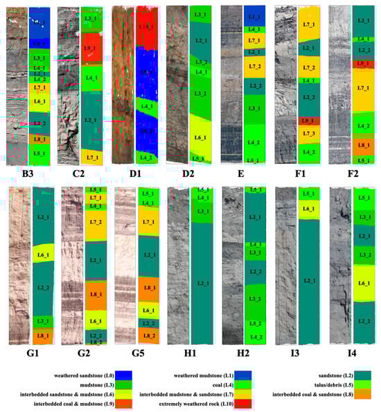
Figure 1. A few annotated samples from the mine highwall dataset (MHD). L1–L10 denote the different layers, while L1_1–L1_X denote the multiple instances of the same layer.

2.3. Data Pre-Processing

The pre-processing of 3D point cloud data involved several steps to ensure efficient training and segmentation of the rock lithology. An overview of the detailed data pre-processing pipeline is presented in Figure 2.

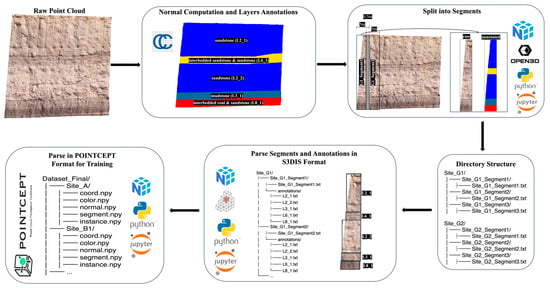
Figure 2. Flow diagram for the data pre-processing pipeline.

In the first step, surface normals were computed for each site using a nearest-neighbour approach while keeping other parameters at their default settings. Surface normals were computed in CloudCompare using the recommended default neighbourhood radius ($r$), which is automatically derived from the local point density and average point spacing to provide a scale-adaptive estimate for normal vector computation [25]. This default choice ensures a balanced trade-off between geometric detail and noise robustness, while acknowledging that the sensitivity of normal estimation to varying $r$ values lies beyond the scope of this study. This step provided essential geometric information for subsequent segmentation and classification tasks.

To manage computational complexity, each site was randomly subdivided into smaller sub-sites, resulting in a total of 35 sites. Each site was then exported as a .txt file containing the attributes $\left[X, Y, Z, R, G, B, Scalar, N_x, N_y, N_z\right]$, where $X$, $Y$, and $Z$ represent spatial coordinates, $R$, $G$, and $B$ denote colour values, Scalar corresponds to layer annotation, and $N_x$, $N_y$, and $N_z$ define the components of the computed surface normals. These features capture both geometric and visual information from the dataset. In addition, the 3D segmentation models employed were originally trained on benchmark point cloud datasets, where these features serve as default input. Maintaining this configuration will allow the models to fully exploit their designed feature extraction mechanisms, ensuring optimal segmentation performance.

For training purposes, each site was further divided into smaller segments to facilitate localised feature learning. A custom script was developed to segment each site into 5 m chunks with an overlapping region of $0.5 \mathrm{m}$, ensuring continuity between adjacent segments. This process resulted in a total of 1498 segments (see Table 1 for detailed site-wise distribution). Site A contributed the fewest segments, with only 9, indicating a relatively small survey area. In contrast, the highest number of segments came from Site I, which provided 392 segments, followed closely by Site H with 318 and Site G with 302, together accounting for the majority of the dataset. Overall, most sites contributed between 40 and 170 segments, making this range the most common across the dataset, with the average per site being approximately 166 segments. In terms of data distribution across the two different data capturing methods, photogrammetry-based data were collected from seven sites (Site A–Site G), contributing a total of 938 segments that include a diverse range of geological conditions and surface morphologies. In contrast, TLS-derived data were obtained from two sites only (Site H and Site I), contributing 560 segments covering material layers L2–L8 only.

Following segmentation, the dataset was converted into a format compatible with the Pointcept library for training Transformer-based 3D segmentation models. The dataset was first reformatted to a widely adopted standard, the Stanford Large-Scale 3D Indoor Spaces Dataset (S3DIS) structure [26], using a custom Python v3.8 script (see Appendix A.1. for pseudocode). Each annotated point cloud corresponding to a specific layer was saved as a separate .txt file, using a naming convention that distinguishes multiple instances of the same layer (e.g., L1_1, L1_2). Subsequently, the Pointcept v1.6.0 dataset processing script [27] was modified to parse the S3DIS-formatted data into the Pointcept format (see Appendix A.2. for pseudocode). This final dataset structure was then used for model training and evaluation.

The overall layer-wise distribution of the MHD dataset is shown in Figure 3, which indicates that sandstone (L2), coal (L4) and talus/debris (L5) have the highest percentage of segments, while weathered mudstone (L1) and extremely weathered rock (L10) have the fewest. This indicates some class imbalance in the dataset. The violin plots in Figure 4 illustrate the distribution of the number of points per instance across different material layers in the dataset, providing insights into data variability and class imbalance. Each violin represents a material layer (L0–L10), with the width of the plot at different heights, indicating the density of instances having that specific point count. Layers such as weathered mudstone (L1), sandstone (L2), talus/debris (L5), and interbedded coal & mudstone (L9) exhibit significant variability, with long tails and wide distributions, suggesting that these layers contain instances ranging from very small to extremely large, possibly due to geological heterogeneity or inconsistencies in point cloud coverage. In contrast, layers like weathered sandstone (L0), mudstone (L3), coal (L4) and interbedded sandstone & mudstone (L6) show more consistent instance sizes, implying consistent exposure. Some layers, such as interbedded coal & sandstone (L8) and extremely weathered rock (L10), appear to have uniformly small instances or occur less frequently, which may be due to thin formations or partial data coverage. Notably, interbedded mudstone & sandstone (L7) shows a bimodal distribution, indicating the presence of two distinct populations of instance sizes, potentially due to merged sub-layers or varying exposure conditions.

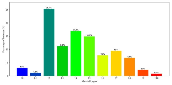
Figure 3. Layer-wise distribution of pre-processed mine highwall dataset (MHD).

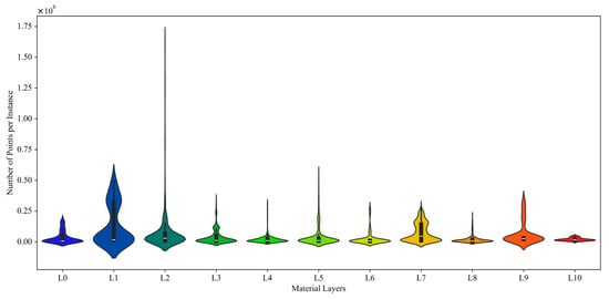
Figure 4. Violin plot for the pre-processed mine highwall dataset (MHD).

2.4. Deep Learning Based 3D Segmentation Models

2.4.1. SparseUNet (SPUNet)

SPUNet is designed to efficiently process large-scale 3D point clouds by leveraging sparse convolutional neural networks, which operate only on non-empty voxels, significantly reducing computational overhead [20]. Unlike traditional 3D convolution methods, which scale poorly due to cubic growth in computation, SPUNet maintains efficiency and detail through submanifold sparse convolutions that skip unnecessary operations in empty space. The architecture follows a U-Net-inspired encoder–decoder structure (see Figure 5), where the encoder compresses spatial dimensions while learning high-level features, and the decoder progressively upsamples them to recover spatial detail. Skip connections between encoder and decoder layers help preserve fine-grained information, enhancing segmentation accuracy. The design ensures scalability and semantic richness, making SPUNet well-suited for high-resolution 3D semantic segmentation.

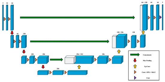
Figure 5. Architecture of the 3D UNet model as the base of SPUNet. Redrawn from [20].

2.4.2. Point Transformer v2 (PTv2)

PTv2 builds upon the original Point Transformer by improving scalability and spatial representation through Grouped Vector Attention (GVA) and enhanced positional encoding [21]. GVA divides feature channels into shared-attention groups, reducing the number of learnable parameters and improving generalisation. To better capture geometric structure, PTv2 introduces a multiplicative position encoding mechanism, which enhances spatial awareness beyond simple bias terms. Additionally, a partition-based pooling strategy replaces conventional sampling methods, aggregating features within fixed spatial partitions. This design improves computational efficiency while preserving local structure, making PTv2 effective for complex 3D scene understanding. Figure 6 shows the basic architecture for the PTv2 model.

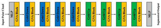
Figure 6. Architecture of the PTv2 model. Redrawn from [21].

2.4.3. Point Transformer v3 (PTv3)

PTv3 shifts focus from attention complexity to scalability and efficiency, achieving significant gains in speed and memory usage [22]. The core innovation is the use of serialised neighbourhoods, where unstructured point clouds are arranged using space-filling curves, enabling structured processing without altering the raw data. Attention computation is simplified through patch-based attention, where local patches replace dynamic neighbour queries. While this risks losing some spatial precision, techniques such as shift-dilation and patch shifting are used to retain cross-patch information flow. PTv3 also replaces relative positional encoding with a lightweight sparse convolution backbone, further improving efficiency. Figure 7 shows the architecture of the PTv3 model. These design choices allow PTv3 to scale to larger scenes while maintaining competitive accuracy.

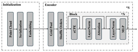
Figure 7. Architecture of the PTv3 model. Redrawn from [22]. (* denotes the “Times” symbol).

2.4.4. Sonata

Sonata [23] is one of the latest state-of-the-art self-supervised learning frameworks designed to overcome the geometric shortcut problem, in which models overfit to low-level spatial cues such as surface normals or point height. The framework instead encourages the learning of high-level, feature-based representations that generalize better across 3D scenes. Built upon the PTv3 backbone (see Figure 7), Sonata removes the traditional decoder to prevent spatial leakage, instead relying on point self-distillation, feature up-casting, and progressive task scheduling to obscure positional bias and enhance semantic understanding. These design choices enable robust, semantically rich representations with exceptional data and parameter efficiency. Notably, Sonata achieves a 3.3 times improvement in linear probing accuracy using less than 0.2% learnable parameters, outperforming previous self-supervised 3D methods.

2.5. Experimental Protocols and Evaluation Measures

The training of all 3D semantic segmentation models for the rock lithology segmentation utilised the PyTorch-based library “Pointcept” [27], which provides an efficient framework for point cloud processing. Open3D v0.19 [28] and CloudCompare [24] facilitated the analysis and visualisation of the segmentation results, enabling a comprehensive evaluation of model performance. The experiments were conducted on an Ubuntu 18.04 machine, equipped with 64 GB RAM and an NVIDIA A6000 GPU with 48 GB VRAM, ensuring sufficient computational resources for training deep learning models. A standard 80:20 holdout dataset split is implemented, where 80% of the data is used for training (i.e., 1197 segments) and 20% (i.e., 281 segments) for evaluation to assess generalisation performance. In terms of training hyperparameters (see Table 3 for definitions), all the models were trained for 300 epochs with a batch size of 4, an initial learning rate of 0.0006 and a validation interval of 10 epochs. The input size to all the models was 6 channels with a grid size of 0.05. The CrossEntropy loss function was used for training all the models with no test time augmentation (TTA). The training pipeline, however, used augmentation including random rotation (along centre, along $x$, along $y$), random scale (0.9,1.1), random flip, random jitter, chromatic auto contrast, chromatic translation, sphere crop and centre shift. A dropout ratio of 20% was used in training to avoid overfitting. Table 4 presents the distinct hyperparameters configured for each model during training.

Table 3. Definitions of training hyperparameters.

Hyperparameter	Definition
Epoch	An epoch refers to one full cycle through the entire training dataset, allowing the model to learn from all samples once.
Batch size	The number of training examples processed together in one forward/backward pass.
Learning rate	A scalar that determines the step size at each iteration while moving toward a minimum of the loss function.
Loss function	A mathematical function that measures the difference between predicted output and true labels.
Optimiser	An algorithm used to adjust model weights based on gradients computed from the loss function.
Dropout	A regularisation technique that randomly sets a fraction of neurons to zero during training to reduce overfitting and improve generalisation.
Backbone	The core feature extractor network used in a deep learning model to capture key representations from input data.
LR Scheduler	A mechanism that adjusts the learning rate during training based on a predefined schedule or training progress to improve convergence.

Table 4. Distinct hyperparameters for 3D segmentation models.

	SPUNet	PTv2	PTv3	Sonata
Optimiser	SGD	AdamW	AdamW	AdamW
BackBone	PointTransformer-Seg50	PT-v2m1	PT-v3m1	PT-v3m2
Trainable Parameters	39,156,971	3,908,543	46,190,423	124,793,563
LR Scheduler	PolyLR	MultiStepLR	OneCycleLR	OneCycleLR

The performance of the 3D segmentation models is evaluated using a combination of quantitative and visual measures from the training and validation phases. The quantitative evaluation includes the mean intersection over union (mIoU) and mean accuracy. The mIoU measures the average intersection over union for all classes, quantifying the overlap between predicted and ground truth segments across the dataset. Mean accuracy represents the average per-class accuracy, ensuring that performance is not biased toward dominant classes. Total accuracy calculates the overall proportion of correctly classified points in the dataset. The visual assessment includes training loss plots, validation mIoU plots, and confusion matrices, which help analyse model learning behaviour and classification performance.

3. Results and Discussion

Figure 8 shows the training loss curves for the trained SPUNet, PTv2, PTv3 and Sonata models applied to the 3D segmentation task for the rock lithology segmentation. The $x$-axis represents the training iterations, while the $y$-axis shows the loss value, reflecting the model’s error during training. Initially, all models exhibit high loss values, which decrease progressively as training continues (i.e., follow a negative exponential curve). SPUNet and Sonata, however, demonstrate relatively higher and more erratic loss values, indicating that they face greater difficulty in effectively learning complex geometric features. In contrast, PTv2 exhibits the most consistent and rapid decrease in loss, converging faster and reaching a lower final loss (i.e., 0.2028) compared to Sonata (i.e., 0.6587), SPUNet (i.e., 0.6534) and PTv3 (i.e., 0.2756). PTv3 achieves comparable performance to PTv2 and shows stable loss convergence, indicating an efficient training process. The validation mIoU curves (see Figure 9), however, demonstrate that PTv3 consistently outperforms the other methods with a significant margin (Sonata by $\approx$21%, PTv2 by $\approx$26% and SPUNet by $\approx$55%) on the validation dataset, indicating that PTv2 may suffer from overfitting to the training data and did not generalise during training. PTv3, though it exhibits slightly higher training loss, benefits from stronger regularisation or an architectural design that encourages learning more generalisable representations. This enables PTv3 to perform better on the validation set.

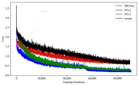
Figure 8. Training loss curves of the trained 3D segmentation models for rock lithology segmentation.

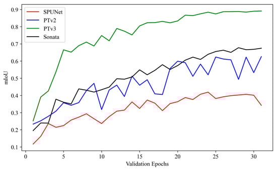
Figure 9. Validation mIoU curves of the trained 3D segmentation models for rock lithology segmentation.

Quantitatively, the PTv3 model achieved a mIoU of 0.8912 and a mAcc of 0.9497, outperforming the second-best model, Sonata, by 21% in mIoU and 15% in mAcc (see Table 5). In terms of per-class performance, for the best-performing model (i.e., PTv3), the highest IoU values are observed for weathered mudstone (L1), sandstone (L2), and debris (L5), with scores of 0.9521, 0.9438, and 0.9342, respectively. In contrast, the lowest IoU values are recorded for coal (L4) and weathered sandstone (L0), with scores of 0.8090 and 0.8390, respectively.

Table 5. Summary of quantitative results of the trained 3D segmentation models for material layers segmentation.

Class	SPUNet		PTv2		PTv3		Sonata
	IoU	Acc	IoU	Acc	IoU	Acc	IoU	Acc
L0	0.2515	0.3837	0.4736	0.5843	0.8390	0.9630	0.4966	0.6925
L1	0.2325	0.2570	0.8358	0.9441	0.9521	0.9600	0.7622	0.8118
L2	0.5524	0.8190	0.8738	0.9555	0.9438	0.9690	0.8414	0.8945
L3	0.3716	0.6330	0.7215	0.8914	0.8879	0.9205	0.6280	0.7751
L4	0.3497	0.4470	0.6237	0.8592	0.8090	0.9029	0.5482	0.6883
L5	0.7198	0.8507	0.8753	0.9247	0.9342	0.9664	0.9064	0.9390
L6	0.1947	0.3024	0.7159	0.8020	0.8966	0.9589	0.7673	0.8867
L7	0.3028	0.3638	0.8066	0.8578	0.9244	0.9584	0.6915	0.8643
L8	0.2464	0.3121	0.7503	0.8144	0.8907	0.9534	0.6612	0.8914
L9	0.0018	0.0018	0.1349	0.1378	0.8573	0.9472	0.5937	0.7733
L10	0.5426	0.7210	0.0743	0.0746	0.8686	0.9474	0.5256	0.5429
Mean	0.3423	0.4629	0.6260	0.7132	0.8912 *	0.9497 *	0.6747	0.7963

* Bold values indicate best performance.

The computational efficiency of the trained 3D segmentation models was evaluated in terms of both training and inference performance, providing a relative comparison across the different architectures. Table 6 summarises the quantitative results, while Figure 10 presents a visual bar graph representation. It can be observed that the conventional SPUNet model exhibits the shortest training time per epoch (i.e., 160.45 s) and the fastest inference time per million points (i.e., 2.27 s). However, despite its computational efficiency, SPUNet demonstrated the poorest segmentation performance, highlighting the trade-off between speed and accuracy. PTv3 achieved a favourable balance between accuracy and inference efficiency. It recorded an inference time of 5.37 s per million points (second only to SPUNet) while requiring 253.94 s per epoch for training, indicating higher computational demand during model optimisation. PTv2, in contrast, exhibited the longest training time per epoch (i.e., 262.17 s) and inference time per million points (i.e., 18.31 s), reflecting its heavier computational overhead. Sonata showed intermediate behaviour, with moderate training time per epoch (i.e., 168.14 s) and inference time per million points (6.99 s), while achieving performance comparable to the other transformer-based models. All measurements were conducted on an NVIDIA A6000 GPU with 48 GB VRAM, and the results are intended for relative comparison rather than absolute benchmarking.

Table 6. Training and inference computational efficiency of the trained 3D segmentation models for material layers segmentation recorded for NVIDIA A6000 GPU with 48 GB VRAM.

	SPUNet	PTv2	PTv3	Sonata
Training Time per Epoch (sec)	160.45	262.17	253.94	168.14
Inference Time per Million Points (sec)	2.27	18.31	5.37	6.99

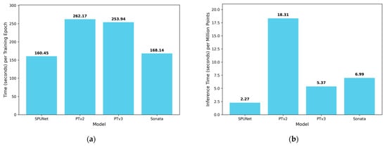
Figure 10. Bar chart representation of the training and inference computational efficiencies of the trained 3D segmentation models for material layers segmentation. (a) Training. (b) Inference.

Figure 11 presents the confusion matrices for the trained models, illustrating the class-wise performance of each model. Overall, PTv3 demonstrates the highest classification accuracy, with the fewest misclassifications. The impact of dataset imbalance is evident in the observed misclassifications. Specifically, for PTv2 and Sonata, the lowest segmentation performance occurs for classes weathered sandstone (L0), interbedded coal & mudstone (L9), and extremely weathered rock (L10), which are all underrepresented in the dataset. This highlights the influence of class frequency on model accuracy and underscores the need for more balanced training data to improve performance across all lithological classes. For the best-performing PTv3, notably, most misclassification instances involve confusion between sandstone (L2) and coal (L4), with approximately 5% of coal (L4) samples incorrectly predicted as sandstone (L2). This trend may be attributed to the frequent adjacency of these two layers in the training dataset, which could have influenced the model’s ability to distinguish between them.

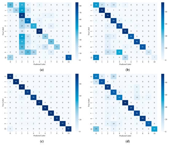
Figure 11. Confusion matrices of the trained 3D segmentation models for rock lithology segmentation: (a) SPUNet, (b) PTv2, (c) PTv3, and (d) Sonata.

Figure 12 displays the visualised predictions of the trained models across selected sites. The visualisations are organised sequentially, presenting the RGB images, corresponding ground truth, and model predictions side-by-side to facilitate a clearer comparison of model performance. From the results, it is evident that PTv3 outperforms the other models by a significant margin, while SPUNet exhibits the poorest performance, with highly scattered and inconsistent predictions. For PTv3, most misclassifications are observed near the layer boundaries.

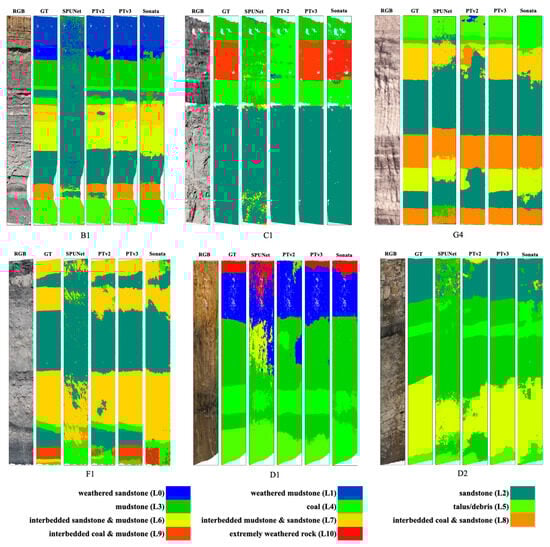
Figure 12. Visualisation of trained 3D segmentation model predictions for rock lithology segmentation.

Figure 13 shows the Principal Component Analysis (PCA) learned embedding visualisations of segmentation model outputs across three random samples from the validation dataset split. PTv3 consistently demonstrates well-separated and compact clusters in the reduced PCA space, suggesting strong intra-class feature cohesion and inter-class discriminability. Sonata also demonstrated comparable performance to PTv3 with clear clusters. In contrast, SPUNet exhibits substantial overlap between classes, with more diffuse clusters, particularly in Sample 1 and Sample 3. This dispersion indicates weaker semantic boundary learning and a less discriminative latent space, likely due to SPUNet’s reliance on sparse convolutions, which, while computationally efficient, may limit the model’s capacity to capture fine-grained contextual relationships. PTv2 presents an intermediate behaviour as it offers slightly improved cluster separability compared to SPUNet, but does not match the compactness and clarity observed in PTv3. This could be attributed to architectural limitations in PTv2’s attention mechanisms, which may not fully capture long-range dependencies or multi-scale context as effectively as PTv3.

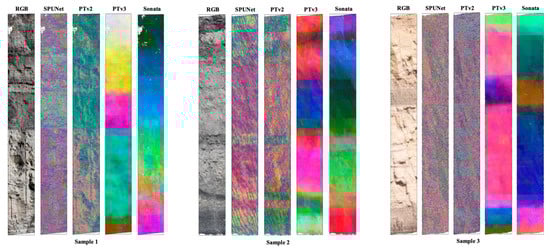
Figure 13. PCA visualisation of feature embeddings generated by segmentation models illustrating feature separability and clustering quality.

The performance of the PTv3 model was further evaluated on separate photogrammetry and TLS validation dataset splits to assess the impact of different data acquisition sources. Figure 14 presents the confusion matrices for both splits. Overall, the model demonstrated slightly better and more stable performance on the photogrammetry data compared to the TLS data. Specifically, the photogrammetry results followed the trend observed in the combined confusion matrix, with the lowest accuracy for L3 and L4, and with L4 frequently misclassified as L2. In contrast, the TLS validation data exhibited the highest misclassification rates for interbedded sandstone & mudstone (L6) and interbedded coal & sandstone (L8). L6 was often misclassified as talus/debris (L5) or sandstone (L2), while L8 was frequently misclassified as L5. These misclassifications can be attributed to the characteristics of TLS scans and the geological nature of the layers. TLS primarily captures geometric and structural features (e.g., 3D shape, surface roughness) and records intensity-based pseudo-RGB values that differ from true colour imagery, generally exhibiting lower quality than photogrammetric data. Interbedded layers like L6 and L8 have heterogeneous compositions and fine stratification, which can be smoothed or underrepresented in TLS point clouds, causing them to resemble simpler layers. Additionally, the surface geometries of these interbedded layers may be similar to unconsolidated debris (L5), and the emphasis on one material over another due to surface exposure or scan orientation may further contribute to confusion with L2 or L5. By contrast, photogrammetry provides higher-quality RGB information that enhances the distinction of interbedded layers, reducing misclassifications. The slightly better performance on photogrammetry data can be attributed to both the higher-quality RGB information, which improves material layer discrimination, and the fact that the dataset contains many more photogrammetry sites than TLS sites, introducing a potential imbalance.

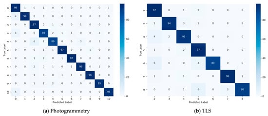
Figure 14. Validation performance of PTv3 model for photogrammetry and TLS data samples for studying the impact of different data sources.

The superior performance of PTv3 compared to Sonata, PTv2 and SPUNet can be attributed to several architectural advantages. PTv3 likely incorporates more effective feature extraction mechanisms that capture multiscale contextual information, which is critical in geotechnical datasets where material layers often exhibit subtle texture and geometric differences. Its consistent performance on the validation set, despite slightly higher training loss, suggests stronger regularisation and a better balance between model complexity and generalisation. This balance enables PTv3 to learn robust, transferable representations rather than overfitting to the specific characteristics of the training data, an issue that appears to have affected PTv2. The minor misclassifications observed near layer boundaries for PTv3 are likely due to the model’s sensitivity to local heterogeneities, small-scale surface irregularities, and noise in the training data.

On the other hand, the poor performance of SPUNet points to limitations in its ability to model complex 3D structures. The higher and unstable training loss trajectory indicates that SPUNet struggled with convergence, likely due to insufficient model capacity or less effective handling of local geometric variations. Unlike PT architectures, SPUNet may lack mechanisms to effectively aggregate fine-grained spatial cues over multiple scales, making it particularly vulnerable in tasks that require detailed boundary delineation, such as rock lithology segmentation. Additionally, the scattered nature of SPUNet’s predictions suggests that it may be more sensitive to noise and minor irregularities in the input data, leading to fragmented and inconsistent outputs.

While the presented models, particularly PTv3, demonstrated strong segmentation performance, several limitations should be acknowledged. First, the dataset used in this study was relatively limited in terms of the number of sites and geographic diversity, which may constrain the generalisability of the models to more heterogeneous or complex geological contexts worldwide. Additionally, the models were trained and validated on datasets exhibiting specific adjacent layering patterns, which may have implicitly influenced the learning process, leading to challenges when transferring to sites with different structural compositions. Another constraint is the dependence solely on static point cloud data without incorporating complementary information such as multispectral, hyperspectral, or structural priors, which could enhance discrimination between visually similar materials. Transformer-based models, although effective, require substantial memory and processing power, posing challenges for real-time applications or deployment in resource-constrained environments. Moreover, dataset imbalance, with certain material layers being underrepresented, may bias learning outcomes and limit performance in minority classes.

In addition, we analysed the validation samples where the PTv3 model exhibited the lowest performance to identify common patterns in misclassification (see Figure 15). Three main failure cases were observed. First (Failure Case 1), validation samples containing very few points, typically clipped portions from the edges, exhibited higher rates of misclassification. This issue could be mitigated in future work by implementing a preprocessing workflow that excludes segments with fewer points than a predetermined threshold. Second (Failure Case 2), misclassification was observed across the boundaries of different material layers, arising from simplified boundary annotations and the inherent similarity of adjacent layers. This limitation could be addressed by expanding the dataset with more distinctive examples and improving annotation quality to capture more precise layer boundaries. Third (Failure Case 3), thin layers with very few points were misclassified to either the adjacent layer or the dominant layer in the sample. This failure could be alleviated by incorporating higher-resolution scans and augmenting the dataset with additional examples of thin layers.

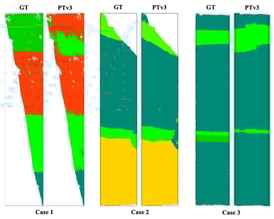
Figure 15. A few representative validation failure cases where PTv3 did not perform well.

Despite its current limitations in generalisation due to the lack of training data from a diverse range of sites, the trained 3D segmentation model can serve as a foundational or base model for rock lithology segmentation. When fine-tuned using a relatively small set of annotated samples from a new site, the base model is expected to generalise well and automatically segment rock lithology across the rest of the site. This transferability significantly reduces the manual annotation effort required at new locations, demonstrating the practical applicability of the proposed solution.

4. Conclusions

The study presents a deep learning-based semantic segmentation approach for rock lithology segmentation in 3D point clouds of open-pit mine highwalls. Four state-of-the-art 3D segmentation models (i.e., SPUNet, PTv2, PTv3, Sonata) were trained using a high-resolution 3D point cloud dataset (i.e., MHD) generated from nine diverse mine sites from NSW and Queensland, Australia. A quantitative evaluation demonstrates that PTv3 significantly outperforms the other models, achieving a mIoU of 0.8912 and mAcc of 0.9497. PTv3’s superior performance is attributed to its multiscale attention mechanisms and efficient representation of local and global spatial dependencies, which enabled better delineation of complex material boundaries. PTv2 and Sonata also achieve reasonable accuracy (mIoU = 0.6260 for PTv2 and mIoU = 0.6747 for Sonata, mAcc = 0.7132 for PTv2, mAcc = 0.7963 for Sonata) but exhibit signs of overfitting, while SPUNet suffers from convergence instability, resulting in comparatively lower segmentation quality (mIoU = 0.3423, mAcc = 0.4629). Visual results further confirm PTv3’s superior performance in rock lithology segmentation. Despite the promising performance of PTv3, limitations such as dataset size, class imbalance, and reliance on static point clouds constrain generalisability and boundary accuracy. It is anticipated that adding data from more diverse sites will enhance the generalisation of the segmentation model. Future work could explore the development of domain-adaptive models, integrating multiple data modalities (e.g., hyperspectral) and addressing the class imbalance problem towards enhancing the robustness of the existing model.

The outcomes of this study establish a foundation for developing lithology-informed digital twins of rock slopes, enabling data-driven rockfall hazard assessment and slope stability analysis. By associating segmented lithological layers with their respective material properties, a spatially resolved digital representation of the rock slope can be established. Such lithology-informed digital twins will enable more reliable prediction of slope responses to external factors (e.g., rainfall, excavation, blasting), thereby enhancing early warning and risk mitigation capabilities. Beyond hazard assessment, the derived lithological information can also be used for facilitating optimised operational planning and long-term monitoring, ultimately improving the safety, efficiency, and sustainability of geotechnical and mining operations.

Appendix A.1. Pseudocode to Extract Layer Annotations

Appendix A.2. Pseudocode to Parse the Data into Pointcept Training Format

References

- Akbulut, N.K.; Anani, A.; Brown, L.D.; Wellman, E.C.; Adewuyi, S.O. Building a 3D Digital Twin for Geotechnical Monitoring at San Xavier Mine. Rock Mech. Rock Eng. 2024, 1–18. [Google Scholar] [CrossRef]
- Ando, A.; Gidaris, S.; Bursuc, A.; Puy, G.; Boulch, A.; Marlet, R. Rangevit: Towards vision transformers for 3d semantic segmentation in autonomous driving. In Proceedings of the IEEE/CVF Conference on Computer Vision and Pattern Recognition, Vancouver, BC, Canada, 17–24 June 2023. [Google Scholar]
- Armeni, I.; Sener, O.; Zamir, A.R.; Jiang, H.; Brilakis, I.; Fischer, M.; Savarese, S. 3d semantic parsing of large-scale indoor spaces. In Proceedings of the 2016 IEEE Conference on Computer Vision and Pattern Recognition (CVPR), Las Vegas, NV, USA, 27–30 June 2016. [Google Scholar]
- Bahootoroody, F.; Giacomini, A.; Guccione, D.E.; Thoeni, K.; Watman, A.; Griffiths, D.V. Predictive Modelling of Rainfall-Induced Rockfall: A Copula-Based Approach. Georisk Assess. Manag. Risk Eng. Syst. Geohazards 2025, 1–13. [Google Scholar] [CrossRef]
- Chen, G.; Deng, W.; Lin, M.; Lv, J. Slope stability analysis based on convolutional neural network and digital twin. Nat. Hazards 2023, 118, 1427–1443. [Google Scholar] [CrossRef]
- CloudCompare Wiki. Normals\Compute. 2024. Available online: https://cloudcompare.org/doc/wiki/index.php/Normals%5CCompute (accessed on 10 November 2025).
- Ferrero, A.M.; Forlani, G.; Roncella, R.; Voyat, H. Advanced geostructural survey methods applied to rock mass characterization. Rock. Mech. Rock. Eng. 2009, 42, 631–665. [Google Scholar] [CrossRef]
- Girardeau-Montaut, D. CloudCompare. Fr. EDF RD Telecom ParisTech. 2016, 11, 2016. [Google Scholar]
- Humair, F.; Abellan, A.; Carrea, D.; Matasci, B.; Epard, J.-L.; Jaboyedoff, M. Geological layers detection and characterisation using high resolution 3D point clouds: Example of a box-fold in the Swiss Jura Mountains. Eur. J. Remote Sens. 2015, 48, 541–568. [Google Scholar] [CrossRef]
- Ibrahim, M.; Akhtar, N.; Anwar, S.; Mian, A. SAT3D: Slot attention transformer for 3D point cloud semantic segmentation. IEEE Trans. Intell. Transp. Syst. 2023, 24, 5456–5466. [Google Scholar] [CrossRef]
- Idrees, M.O.; Pradhan, B. A decade of modern cave surveying with terrestrial laser scanning: A review of sensors, method and application development. Int. J. Speleol. 2016, 45, 71. [Google Scholar] [CrossRef]
- Jing, R.; Shao, Y.; Zeng, Q.; Liu, Y.; Wei, W.; Gan, B.; Duan, X. Multimodal feature integration network for lithology identification from point cloud data. Comput. Geosci. 2025, 194, 105775. [Google Scholar] [CrossRef]
- Li, J.; Yang, T.; Liu, F.; Zhao, Y.; Liu, H.; Deng, W.; Gao, Y.; Li, H. Modeling spatial variability of mechanical parameters of layered rock masses and its application in slope optimization at the open-pit mine. Int. J. Rock. Mech. Min. Sci. 2024, 181, 105859. [Google Scholar] [CrossRef]
- Pointcept Contributors. Pointcept: A Codebase for Point Cloud Perception Research. 2023. Available online: https://github.com/Pointcept/Pointcept (accessed on 27 October 2025).
- Robiati, C.; Mastrantoni, G.; Francioni, M.; Eyre, M.; Coggan, J.; Mazzanti, P. Contribution of High-Resolution Digital Twins for the Definition of Rockfall Activity and Associated Hazard Modelling. Land 2023, 12, 191. [Google Scholar] [CrossRef]
- Singh, S.K.; Banerjee, B.P.; Raval, S. A review of laser scanning for geological and geotechnical applications in underground mining. Int. J. Min. Sci. Technol. 2023, 33, 133–154. [Google Scholar] [CrossRef]
- Tan, W.; Wu, S.; Li, Y.; Guo, Q. Digital Twins’ Application for Geotechnical Engineering: A Review of Current Status and Future Directions in China. Appl. Sci. 2025, 15, 8229. [Google Scholar] [CrossRef]
- Thoeni, K.; Santise, M.; Guccione, D.E.; Fityus, S.; Roncella, R.; Giacomini, A. Use of low-cost terrestrial and aerial imaging sensors for geotechnical applications. Aust. Geomech. J. 2018, 53, 101–122. [Google Scholar]
- Ugur, M.; Ustaoglu, A.O.; Yasin, B.; Ilyas, Y.; Sultan, K.; Candan, G. Rockfall Hazard Assessment for Natural and Cultural Heritage Site: Close Vicinity of Rumkale (Gaziantep, Türkiye) Using Digital Twins. Heritage 2025, 8, 270. [Google Scholar] [CrossRef]
- Wang, B.; Mohajerpoor, R.; Cai, C.; Kim, I.; Vu, H.L. Traffic4cast--Large-scale Traffic Prediction using 3DResNet and Sparse-UNet. arXiv 2021, arXiv:2111.05990. [Google Scholar]
- Wu, X.; DeTone, D.; Frost, D.; Shen, T.; Xie, C.; Yang, N.; Engel, J.; Newcombe, R.; Zhao, H.; Straub, J. Sonata: Self-Supervised Learning of Reliable Point Representations. In Proceedings of the Computer Vision and Pattern Recognition Conference, Nashville, TN, USA, 10–17 June 2025; pp. 22193–22204. [Google Scholar]
- Wu, X.; Jiang, L.; Wang, P.-S.; Liu, Z.; Liu, X.; Qiao, Y.; Ouyang, W.; He, T.; Zhao, H. Point transformer v3: Simpler faster stronger. In Proceedings of the IEEE/CVF Conference on Computer Vision and Pattern Recognition (CVPR), Seattle, WA, USA, 17–18 June 2024; pp. 4840–4851. [Google Scholar]
- Wu, X.; Lao, Y.; Jiang, L.; Liu, X.; Zhao, H. Point transformer v2: Grouped vector attention and partition-based pooling. Adv. Neural Inf. Process. Syst. 2022, 35, 33330–33342. [Google Scholar]
- Wyllie, D.C.; Mah, C. Rock Slope Engineering; CRC Press: Boca Raton, FL, USA, 2024. [Google Scholar]
- Xu, J.; Zhang, Y. AI-Powered Digital Twin Technology for Highway System Slope Stability Risk Monitoring. Geotechnics 2025, 5, 19. [Google Scholar] [CrossRef]
- Yang, B.; Haala, N.; Dong, Z. Progress and perspectives of point cloud intelligence. Geo-Spat. Inf. Sci. 2023, 26, 189–205. [Google Scholar] [CrossRef]
- Yue, Z.; Yue, X.; Wang, X.; Li, Y.; Li, W.; Dai, S.; Gan, L. Experimental study on identification of layered rock mass interface along the borehole while drilling. Bull. Eng. Geol. Environ. 2022, 81, 353. [Google Scholar] [CrossRef]
- Zhou, Q.-Y.; Park, J.; Koltun, V. Open3D: A modern library for 3D data processing. arXiv 2018, arXiv:1801.09847. [Google Scholar] [CrossRef]
Disclaimer/Publisher’s Note: The statements, opinions and data contained in all publications are solely those of the individual author(s) and contributor(s) and not of MDPI and/or the editor(s). MDPI and/or the editor(s) disclaim responsibility for any injury to people or property resulting from any ideas, methods, instructions or products referred to in the content. |
© 2025 by the authors. Licensee MDPI, Basel, Switzerland. This article is an open access article distributed under the terms and conditions of the Creative Commons Attribution (CC BY) license (https://creativecommons.org/licenses/by/4.0/).