Analysis of Regional Surface CO₂ Fluxes Using the MEGA Satellite Data Assimilation System

Highlights

What are the main findings?

• This study develops the MEGA system that combines Lagrangian and Eulerian models at 1° × 1° spatial and 3-h temporal resolution, assimilating OCO-2 V11.1r XCO₂, and estimates a China terrestrial natural carbon sink of 0.28 ± 0.15 PgC yr⁻¹ during 2018 to 2023, consistent with other inversion systems.
• Six prior sensitivity experiments showed high consistency, indicating that satellite observations provide strong constraints on the results based on the MEGA inversion system.
• Ten background field sensitivity tests show that model-based backgrounds better reproduce the amplitude and phase of the seasonal cycle, especially during July−August, and they reveal the effects of initial fields, flux fields, and mask resolution on the inversion results.

What are the implications of the main findings?

• MEGA offers a robust and near-real-time regional carbon flux inversion tool that complements and strengthens existing regional inversion systems and can be extended to other countries and regions to support policy assessment and mitigation monitoring.
• The model-based background field could provide a more reliable framework for seasonal signal characterization in satellite data assimilation.

Abstract

Understanding the dynamics of terrestrial carbon sources and sinks is crucial for addressing climate change, yet significant uncertainties remain at regional scales. We developed the Monitoring and Evaluation of Greenhouse gAs Flux (MEGA) inversion system with satellite data assimilation and applied it to China using OCO-2 V11.1r XCO₂ retrievals. Our results show that China’s terrestrial ecosystems acted as a carbon sink of 0.28 ± 0.15 PgC yr⁻¹ during 2018–2023, consistent with other inversion estimates. Validation against surface CO₂ flask measurements demonstrated significant improvement, with RMSE and MAE reduced by 30%–46% and 24–44%, respectively. Six sets of prior sensitivity experiments conclusively demonstrated the robustness of MEGA. In addition, this study is the first to systematically compare model-derived and observation-based background fields in satellite data assimilation. Ten sets of background sensitivity experiments revealed that model-based background fields exhibit superior capability in resolving seasonal flux dynamics, though their performance remains contingent on three key factors: (1) initial fields, (2) flux fields, and (3) flux masks (used to control regional flux switches). These findings highlight the potential for further refinement of the atmospheric inversion system.

1. Introduction

In 2023, the concentration of carbon dioxide (CO₂) in the atmosphere climbed to 420 ppm, marking an 11% increase over the last 20 years [1]. This rise exacerbates the greenhouse effect, significantly contributing to global warming [2]. The global terrestrial carbon sink plays a critical role by absorbing roughly one-third of the CO₂ emissions generated by fossil fuel and cement emissions, thus influencing the global carbon budget. Atmospheric inversion stands out as a pivotal technique for estimating terrestrial carbon sinks across scales, from global to regional. This method deduces carbon fluxes by analyzing the spatial and temporal gradients of CO₂ concentrations [3]. Within a Bayesian framework, atmospheric transport models are used to adjust prior carbon flux estimates, ensuring that they align with observed CO₂ concentrations while accounting for the uncertainties in both prior fluxes and observations [4].

In recent decades, numerous global CO₂ atmospheric inversion systems have been established, generally providing consistent estimates of global net carbon fluxes [5,6,7,8]. However, significant discrepancies arise when assessing terrestrial carbon sinks at regional scales [9]. For instance, despite multiple studies on Australia’s terrestrial carbon fluxes, there remains no consensus on whether these ecosystems act as a carbon source or sink [10]. A similar challenge is faced in estimating China’s terrestrial carbon sink, with previous research showing estimates ranging from 0.16 to 1.1 PgC yr⁻¹—an over 600% variance [11,12]. Smaller regions face even greater challenges in accurately assessing their carbon sinks, which complicates the development of effective carbon offset and reduction strategies. Therefore, minimizing uncertainties of the regional carbon sink is crucial for evidence-based policy-making and environmental governance.

The significant divergence in regional carbon sink inversion results primarily stems from systematic differences in inversion parameters (e.g., observations and transport model). For instance, two studies utilizing the same CarbonTracker 2022 (CT2022) inversion system estimated China’s carbon sink as 0.16 PgC yr⁻¹ (2018–2022) [11] and 0.44 PgC yr⁻¹ (2019–2021) [13], respectively, with a difference of 276%. The former relied on in situ observations from global sites [11], while the latter incorporated additional ground-based observations from 30 provinces in China and OCO-2 satellite data [13]. Beyond observations, regional inversion results from different Eulerian models also show substantial discrepancies. For example, the Orbiting Carbon Observatory-2 (OCO-2) model intercomparison project (MIP), which aggregates results from over a dozen inversion systems based on Eulerian frameworks, reveals considerable regional variability and systematic differences among these systems even when assimilating identical OCO-2 observations [14]. This divergence likely arises from transport errors induced by numerical diffusion inherent to Eulerian models. Additionally, most global Eulerian-based inversion systems operate at coarse resolutions (e.g., 4° × 5°), which limits their capability to capture fine-scale regional carbon flux variations. This resolution constraint, combined with numerical diffusion errors, contributes to the substantial discrepancies observed in regional carbon sink estimates. In contrast, the Lagrangian particle dispersion model (LPDM) avoids such numerical diffusion issues.

LPDM has been used extensively at a regional scale since the 2000s [15,16,17]. LPDMs simulate the movement of virtual particles, representing atmospheric gases, from their sources or sinks to receptors, thereby establishing source–receptor relationships (SRRs). Unlike Eulerian models, LPDMs are not affected by numerical diffusion, which often leads to transport errors and non-monotonic behavior in higher-order schemes [18]. This advantage allows LPDMs to more accurately capture synoptic, super-synoptic, and hourly variations without the drawbacks of numerical diffusion [18]. Additionally, LPDMs offer flexibility, as the calculated SRR can be applied to any gas with a lifetime exceeding the back-trajectory timescale. However, LPDMs do have limitations. For long-term studies, they often require background conditions, known as background fields, and simulating these fields over extended periods is computationally intensive. LPDMs lack the computational efficiency of Eulerian models due to the absence of numerical diffusion [19]. This challenge can be mitigated by integrating LPDMs with Eulerian models, combining the strengths of both approaches.

Integrating Eulerian and Lagrangian models presents a promising approach to developing a cost-effective, high-resolution surface flux data assimilation system [19]. Research has explored the coupling of these models on both global and regional scales [20,21]. One study demonstrated that a combined Eulerian–Lagrangian model effectively simulates high-frequency atmospheric CO₂ concentrations worldwide, with notable accuracy at coastal and high-emission locations [18]. Another study on global SF6 emission inversion revealed that the combined model not only aligns well with previous emission estimates in terms of global totals and large-scale patterns but also enhances results resolution and improves the match between modeled and observed mole fractions at certain sites [22]. Additionally, a CO₂ inversion study using the combined model showed improved agreement between modeled and observed CO₂ concentrations at the Samoa and Hateruma sites, with correlation coefficients in fossil fuel emission-driven areas increasing by 0.05 to 0.1 over the 0.5–0.6 range achieved by the Eulerian model alone [19].

One key advantage of the combined model is its ability to operate at higher spatial resolutions than typical Eulerian-based inversion systems. While most global Eulerian models operate at coarse resolutions (e.g., 4° × 5°), the combined model enables flux optimization at finer resolutions (e.g., 1° × 1°) through the flexible selection of flux data resolution for LPDM, independent of the Eulerian model’s simulation grid and flux data resolution. Furthermore, the high-resolution LPDM requires only a single run for each observation or for multiple gases [23], whereas the Eulerian model requires multiple runs. By integrating the strengths of both Lagrangian and Eulerian models, the combined model could significantly lower the expenses associated with multi-species inversions. Moreover, this combined model is versatile and can be applied to any geographical area.

Existing combined models are primarily designed for ground-based observation assimilation, with few dedicated frameworks optimized for satellite observation assimilation. Notably, regional-scale studies reveal that while traditional in situ inversions and biosphere model simulations show greater variability, OCO-2 inversions provide well-constrained mean seasonal cycles in temperate, tropical, and subtropical monsoon regions, particularly demonstrating superior inter-model consistency at sub-regional scales [24]. OCO-2 MIP demonstrates that inversion systems integrating high-density OCO-2 observations achieve a higher error reduction rate at regional and national scales (except for some small high-latitude countries) relative to ground-based systems [14].

Given these significant regional discrepancies and the advantages of Lagrangian models, this study aims to develop a Lagrangian–Eulerian combined model specifically for satellite data assimilation. We propose a method that leverages Lagrangian–Eulerian combined strengths. Utilizing a Bayesian framework, our system assimilates the bias-corrected Orbiting Carbon Observatory-2 (OCO-2) v11.1r column-averaged dry-air mole fraction (XCO₂) retrievals to deduce regional monthly gridded terrestrial CO₂ fluxes for the period 2018–2023. We refer to this system as the Monitoring and Evaluation of Greenhouse gAs Flux (MEGA) inversion system. MEGA can significantly contribute to the ensemble of existing CO₂ inversions and addresses the limited diversity of atmospheric transport models in the OCO-2 MIP. MEGA is specifically optimized for satellite data assimilation, offering enhanced computational efficiency for multi-species inversions. Moreover, MEGA is versatile and can be applied to any region.

In the following sections of this paper, we detail the principles of our assimilation system, MEGA, including the transport models, data inputs, evaluation datasets, inversion parameters (e.g., prior scaling factor, prior uncertainty, etc.), and sensitivity experiment schemes in Section 2. Section 3 focuses on evaluating and analyzing our inversion results, particularly their seasonal cycle variations. Section 4 discusses the outcomes of the prior and background sensitivity tests, along with the limitations and prospects of our assimilation system. Finally, Section 5 provides a summary of the study’s findings.

2. Materials and Methods

We developed a Bayesian-based regional carbon assimilation system that couples the Lagrangian Particle Dispersion Model (LPDM) with a global Eulerian model to infer monthly gridded terrestrial natural carbon fluxes from OCO-2 column-averaged dry-air mole fraction (XCO₂) retrievals. This flux is derived by subtracting the prescribed emissions from fossil fuel emissions from the optimized net carbon flux. An overview of the workflow is shown in Figure 1.

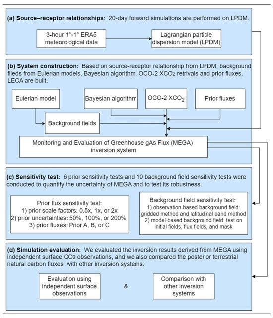
Figure 1. Overview of the Monitoring and Evaluation of Greenhouse gAs Flux (MEGA) inversion system development, sensitivity tests, and evaluation process.

First, we use the LPDM to obtain SRRs (defined in Section 2.2) based on 1$°\times 1°$ 3-h European Centre for Medium-Range Weather Forecasts Reanalysis v5 (ERA5) meteorological data over the research domain. In the second step, we assimilate OCO-2 XCO₂ (introduced in Section 2.4) retrievals processed at 3-h 1$°\times 1°$ resolution using the Bayesian algorithm, the background field obtained from the Eulerian model, and prior carbon fluxes to derive monthly gridded terrestrial carbon fluxes. In this way, we developed the Monitoring and Evaluation of Greenhouse gAs Flux (MEGA) inversion system. After successfully establishing MEGA, we performed six sensitivity experiments using three sets of prior fluxes, different prior scale factors, and varied prior uncertainties; and executed ten sensitivity experiments with five sets of observation-based background fields and five sets of model-based background fields, varying initial fields, flux fields, and masks. To validate the combined model, we evaluated the inversion results based on MEGA using independent surface CO₂ observations and compared the optimized terrestrial natural carbon fluxes from this study with those from multiple carbon assimilation systems, including CarbonTracker2022 CT2022 [2], Global Carbon Assimilation System (GCAS) [3], Copernicus Atmosphere Monitoring Service (CAMS; both satellite-based v23r3 and v24r1 versions) [4], Orbiting Carbon Observatory-2 model intercomparison project (OCO-2 MIP) [5], Jena CarboScope [6], Global Observation-based system for monitoring Greenhouse Gases (GONGGA) [7] and Li et al. [8], and national inventories (see Section 3.2 for details).

2.1. Monitoring and Evaluation of Greenhouse gAs Flux (MEGA) Inversion System

For long-lived trace gases (with lifetimes of several years or more), the assumption of a linear response relationship between atmospheric mole fractions and emission changes is highly effective [22]. By using this linear relationship, we can link the observation vector (y) and the emission vector (x) using the following equation [25]:

$$y=Hx+\epsilon$$

(1)

here $y_{(M \times 1)}$ is the vector of observed mixing ratios at $M$ points in time and space, $x_{(N\times 1)}$ the fluxes state vector of the $N$ state variables discretized in time and space, and $\epsilon$ the sum of observation and model error. $H_{(M\times N)}$ is a matrix of sensitivities of the observations to changes in emissions and is estimated using chemistry transport models, also called the SRR. In this study, $H$ is obtained by running LPDM forward in time.

Bayes’ theorem is used to determine a posteriori fluxes. A prior flux estimates should be added to solve Equation (1) for $x$. The Bayesian inversion method aims to minimize the difference between observed and modeled mixing ratios while keeping the results close to the a priori flux and within predefined uncertainty limits. The uncertainties are assumed to follow a Gaussian distribution, leading to the minimization of the cost function [25]

$$J\left(x\right)={\displaystyle \frac{1}{2}}{\left(x-x_a\right)}^T{S_a}^{-1}\left(x-x_a\right)+{\displaystyle \frac{1}{2}}{\left(Hx-y\right)}^T{S_o}^{-1}\left(Hx-y\right)$$

(2)

where $S_a$ represents the a priori flux error covariance matrix, $S_o$ denotes the observation error covariance matrix, and $x_a$ is the vector of a priori fluxes. $S_o$ is set with reference to the retrieval error for each observation. The detailed construction and setting of $S_a$ and $S_o$ are in the Supplementary Materials. The three-hourly observation error within each grid cell is calculated as the mean retrieval error of all observations in that grid cell over the corresponding three-hour interval. This study employs the following analytical solution to minimize J(x):

$$x = x_a+{\left(H^T{S_o}^{-1}H + {S_a}^{-1}\right)}^{-1}{H}^T{S_o}^{-1}(y-H{x}_a)$$

(3)

where $x$ is a posterior flux that we need. In this study, the terrestrial net carbon fluxes and terrestrial natural carbon fluxes (terrestrial biospheric fluxes plus fire fluxes) are optimized via assimilating OCO-2 XCO₂ retrievals (introduced in Section 2.4) with MEGA. A negative value of terrestrial natural carbon fluxes is equivalent to a carbon sink value. And the uncertainty of posterior flux $x$ depends on the posterior flux error covariance matrix $S_{\mathrm{b}}$:

$$S_b = {\left(H^T{S_o}^{-1}H + {S_a}^{-1}\right)}^{-1}$$

(4)

In forward simulation of LPDMs, virtual particles are usually tracked forward in time for only a few days to weeks. Therefore, the effects of atmospheric transport and surface fluxes from earlier times (called the background mixing ratio field, hereafter referred to as background field) need to be addressed separately. The background field represents the influence of all the emissions or sinks’ contributions before the simulation time period, which has to be defined [26]. There are two general methods to estimate the background field: one is the observation-based method, and the other is the model-based method.

The observation-based method is typically done by selecting observations that represent background air and interpolating between them [16], or by statistically determining an offset to apply to observations over a certain period [15,27]. The issue with the former is that it requires assuming a constant background field over a certain period, yet the background field is strongly influenced by ever-changing meteorological conditions, making constancy nearly impossible. The limitation of the latter is its inability to identify background mole fractions lower than the observed values. This complexity makes it challenging to determine a background field based solely on observations. Model-based approaches address this by linking the meteorology to mixing ratios derived from a global model. While capturing background signals like seasonal changes via forward three-dimensional (3D) simulations in LPDMs, the computational cost is prohibitive [15]. Compared to LPDMs, using global Eulerian models with numerical diffusion is more computationally efficient. Therefore, we chose to use the Eulerian model to obtain the regional background field, and establish a combined model, named Monitoring and Evaluation of Greenhouse gAs Flux (MEGA) inversion system. Additionally, we compare the impact of observation-based and model-based background fields on the inversion results. The scheme of the background field sensitivity test is introduced in Section 2.6.2, and the results are shown in Section 4.1.

The MEGA operates by running the LPDM within a regional domain and coupling it with a global Eulerian model at the research domain boundary. More specifically, we run LPDM forward within a region domain and obtain the forward $H$ operator. Simultaneously, we use a global Eulerian model to calculate the background mixing ratios for each grid daily, enabling us to perform regional-scale inversion on a finer grid using the LPDM. The coupling between the Eulerian and Lagrangian models in MEGA is strictly one-way, with information flowing only from the Eulerian model to the Lagrangian model. There is no feedback of posterior fluxes to the Eulerian background field, and no iterative cycling between the two models is performed. The introduction and operation of the LPDM are covered in Section 2.2, while the Eulerian model used for simulating the background field and its operation is presented in Section 2.3. In this study, we use China as an example to introduce the system and its performance.

2.2. Atmospheric Transport Model

The source–receptor relationship measures emission sensitivity by connecting changes in emissions/sinks within a specific grid cell to alterations in modeled mixing ratios at a designated receptor [28]. In this study, we employ FLEXPART version 10.4 as the LPDM to compute the SRR. The inversion method based on FLEXPART has been widely utilized in previous research [17,29,30,31,32,33,34,35]. Based on FLEXPART version 10.4, we operate FLEXPART in forward mode for 20 days, driven by 3-h ERA5 reanalysis meteorological data from the European Centre for Medium-Range Weather Forecasts (ECMWF), with a spatial resolution of 1$°\times 1°$ and a temporal resolution of 3 h. FLEXPART computes particle trajectories by interpolating three-dimensional meteorological fields from ERA5, which include wind velocity components, air density, temperature, specific humidity, and cloud liquid and ice water content [36]. FLEXPART solves the atmospheric transport equation in a Lagrangian framework by tracking ensembles of particles. The particle position is updated using the Langevin equation, which describes the stochastic movement of particles in turbulent flows [15].

The 20-day forward simulation period was selected based on scientific and computational considerations. CO₂, as a long-lived greenhouse gas, requires sufficient time to trace all potential emission sources. Our testing showed that 10 days is insufficient to cover the complete transport pathway from source regions to satellite observation points, while 20 days adequately captures this transport process. Although longer periods (30+ days) could be used, the computational cost increases exponentially with simulation time in FLEXPART. Therefore, 20 days represents an optimal balance between scientific requirements and computational feasibility.

2.3. The Background Field

In this study, we choose GEOS-Chem to simulate the daily 3D background field. According to the 20-day FLEXPART forward simulation setup in Section 2.2, the background field for a given day (day $i$) is equivalent to the impact of fluxes outside the research domain on the concentration within the domain from 20 days prior (day $i-19$). Therefore, during simulation, we ensure no fluxes within the domain and normal fluxes outside the domain, running for 20 days to obtain the background field for day $i$.

The steps for simulating the background field are shown in Figure 2. First, we conduct a spin-up phase. According to data from the NOAA Global Monitoring Laboratory (https://gml.noaa.gov/ccgg/trends/ (accessed on 21 August 2024)), the global marine surface CO₂ concentration was 395 ppm on 1 January 2013. Thus, we initiate GEOS-Chem with a uniform global concentration of 395 ppm as of 1 January 2013, allowing the model’s transport mechanisms to establish the spatial distribution of CO₂. The spin-up runs from 2013 until the end of 2017. Then, we run GEOS-Chem to obtain the daily background field for each grid for the research area. Due to the long atmospheric lifetime of CO₂, the initial concentrations play a crucial role in shaping the results of GEOS-Chem simulations. The initial global average CO₂ concentration (initial field) exerts a more substantial influence on the simulation outcomes than the distribution patterns of CO₂ [37]. For better simulation, an initial field that more accurately reflects reality is required. In this study, we assume that OCO-2 observations (introduced in Section 2.4) reflect the true CO₂ column concentration changes, but the existing OCO-2 data lack sufficient temporal and spatial coverage to support the construction of a 3D concentration field. Therefore, we calibrate the daily initial field from 13 December 2017 to 31 December 2023, based on processed daily average OCO-2 observations, assuming this initial field closely matches the actual OCO-2 observed concentration field. We call this scaled initial field the OCO-2 scaled initial field. After obtaining the scaled daily initial field, we use a mask to set China’s fluxes to zero while allowing normal fluxes in other regions according to the prior flux field to simulate and obtain the daily 3D background field. The mask is used to control the on/off switch of flux fields in different regions. For example, using the initial field from 13 December 2017, as a restart file in GEOS-Chem, we turn off fluxes in China while maintaining normal fluxes elsewhere, running forward for 20 days to obtain the concentration field for 1 January 2018. To ensure that we only close the grid flux field within the study area, we maintain the spatial resolution of the mask consistent with that of the final posterior results, thus using a 1° $\times$ 1° mask. To reduce computational costs, we run the model at a spatial resolution of 4$°\times 5°$ and then regrid the 4$°\times 5°$ background field to match the 1$°\times 1°$ resolution of the SRR obtained from running FLEXPART. The concentration field extracted for China represents the background field for China. Following this method, we obtain the daily regional background field for each grid in the study area from 2018 to 2023.

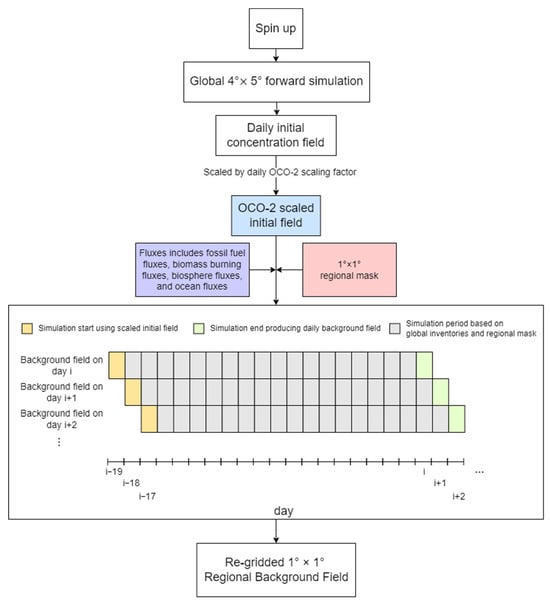
Figure 2. Flowchart of background field simulation based on the Eulerian model in MEGA.

The GEOS-Chem model is a comprehensive global 3D chemical transport model [38] (https://geos-chem.seas.harvard.edu/ (accessed on 1 January 2025)) that leverages meteorological inputs from NASA’s Goddard Earth Observing System (GEOS), courtesy of the Global Modeling and Assimilation Office. This model has been widely adopted by research teams around the globe to construct global carbon inversion systems [39,40,41,42], with differences in model versions, data assimilation methods, and prior fluxes. In our research, we utilize GEOS-Chem v14.2.3 to model global CO₂ transport and connect surface carbon fluxes with observed atmospheric CO₂ gradients, using a horizontal resolution of 4$°$ latitude by 5$°$ longitude, powered by Modern-Era Retrospective Analysis for Research and Applications, version 2 (MERRA-2) meteorological data. This resolution is adept at capturing the large-scale transport of atmospheric CO₂ and its spatiotemporal dynamics, striking a balance between ensemble simulation demands and computational efficiency. And we call this background field the Reference background field in Section 2.6.2.

2.4. Prior Carbon Fluxes and Assimilated OCO-2 Observations

In this system, we utilize four types of prior carbon fluxes, including fossil fuel, biomass burning, ocean, and terrestrial biospheric fluxes. The monthly fossil fuel fluxes for 2018–2023 are sourced from the Open-source Data Inventory for Anthropogenic CO₂ (ODIAC, version 2024) dataset [43]. Biomass burning emissions from 2018 to 2023 were obtained from the Global Fire Emissions Database (GFED5) [44], which provides monthly emissions categorized by fire type, along with daily and 3-hourly temporal profiles. Ocean-atmosphere CO₂ fluxes were sourced from the pCO₂-Clim prior of CarbonTracker version CT2022 [11]. Terrestrial biospheric fluxes were extracted from the Simple Biosphere Model, version 4.2 (SiB4) global hourly dataset [45]. Since CT2022 and SiB4 data were only available up to 2020 and 2018, respectively, we assumed the prior ocean flux for 2021–2023 to be the same as in 2020, and the prior terrestrial flux for 2019–2023 to be the same as in 2018. These fossil fuel, biomass burning, ocean, and terrestrial biospheric fluxes collectively form our prior fluxes, which we designate as Prior A for subsequent sensitivity testing.

In our study, we estimate regional terrestrial net carbon fluxes by assimilating OCO-2 XCO₂ retrievals from the OCO-2 Level 2 (lite file version 11.1) satellite data provided by NASA (https://disc.gsfc.nasa.gov/OCO-2 (accessed on 25 January 2025)). Since its launch in 2014, OCO-2 has delivered high-density XCO₂, proving invaluable for carbon cycle researchers in estimating surface carbon fluxes on both global and regional scales [46]. OCO-2 operates in three modes: nadir, glint, and target. In the nadir mode, the instrument points directly down at the Earth’s surface (with a solar zenith angle less than 85°); in the glint mode, it targets the bright glint spot where solar radiation reflects off the surface (with a local solar zenith angle less than 75°); and in the target mode, it scans around a specific ground point as it passes overhead. In this study, we specifically assimilated the land retrievals, which include both Land Nadir and Land Glint (LNLG) observations. Before integration into the inversion system, the XCO₂ data are filtered using the xCO₂_quality_flag and then re-gridded to a spatial resolution of 1$°\times 1°$ and a temporal resolution of 3 h.

2.5. Auxiliary Data

In this study, we conducted independent validation of inversion results using surface CO₂ observations obtained at the Gosan station from the World Data Centre for Greenhouse Gases (WDCGG; https://gaw.kishou.go.jp/about_wdcgg/wdcgg (accessed on 7 Marth 2025)) and at the Damingshan station [47]. The Gosan station (33°17′N, 126°09′E), located in the East Asian Monsoon region downwind of China, was selected as the primary validation site for its unique capability to capture CO₂ signals influenced by emissions/sinks from continental East Asia [48] (Figure S1a). Observations at Gosan have been extensively utilized in prior studies to quantify regional emissions of greenhouse gases and halogenated compounds [29,49]. The Damingshan station (30°01′N, 119°00′E) is situated in one of China’s most economically developed regions, surrounded predominantly by subtropical evergreen broad-leaved and coniferous forests [47]. A previous study has demonstrated that Damingshan station could capture CO₂ signals influenced by both regional and long-range sources [47] (Figure S1b). While China operates multiple monitoring stations, post-2016 data from most sites remain unpublished. The sole publicly available high-altitude background station, Waliguan, predominantly reflects well-mixed baseline concentrations and exhibits limited sensitivity to CO₂ source-sink dynamics [50]. Consequently, we employed surface observations at Gosan (2018–2023) and Damingshan (September 2020–December 2021) as the independent validation dataset for this analysis.

For the evaluation of our system, we included outputs from four CO₂ inversion systems, including CAMS (Copernicus Atmosphere Monitoring Service), GONGGA (Global Observation-based System for Monitoring Greenhouse Gases), CarbonTracker, and the Orbiting Carbon Observatory-2 (OCO-2) model intercomparison project (MIP). Also, for background field sensitivity tests, we utilized the 3D concentration field from CAMS and CT2022, and optimized flux from GONGGA.

The CAMS CO₂ inversion system optimizes global CO₂ flux estimates by integrating ground-based and satellite observation data. CAMS CO₂ inversion system adopted the global transport model of the Laboratoire de Météorologie Dynamique (LMDz), driven by ERA5 meteorological fields. The inversion relies on a variational formulation of Bayes’ theory. CAMS has released optimized CO₂ flux and concentration products, which are categorized into two main types: one derived from assimilating satellite data [51] and the other from assimilating surface air-sample observations [52]. Both the satellite inversion dataset from CAMS v23r3 (referred to as satellite-based CAMS) and the surface observation inversion dataset (referred to as surface-based CAMS) (https://ads.atmosphere.copernicus.eu/datasets/cams-global-greenhouse-gas-inversion (accessed on 25 January 2025)) were used.

GONGGA obtains gridded global land and ocean carbon fluxes by assimilating OCO-2 XCO₂ observations. The GONGGA system employs the GEOS-Chem atmospheric transport model and utilizes the Nonlinear Least Squares Four-dimensional Variational (NLS-4DVar) inversion method [41]. In this study, we used the latest version of the global 2° × 2.5° three-hourly posterior flux released by GONGGA for background sensitivity test (https://doi.org/10.5281/zenodo.8368846 (accessed on 25 January 2025).

CarbonTracker, developed by the National Oceanic and Atmospheric Administration (NOAA), is a CO₂ measurement and modeling system designed to monitor global CO₂ emissions and sinks. It utilizes atmospheric CO₂ observations and simulated atmospheric transport to estimate surface CO₂ fluxes [11]. In this study, we use the fields of CO₂ mole fraction and posterior carbon fluxes from CT2022 dataset released by CarbonTracker (https://gml.noaa.gov/aftp/products/carbontracker/ (accessed on 25 January 2025)).

OCO-2 MIP unites atmospheric CO₂ modelers to assess the impact of incorporating OCO-2 retrieval data into atmospheric inversion models. In our study, we utilized carbon fluxes from v10 inversions, specifically the LNLG version, which, like our approach, assimilated OCO-2 Land Nadir and Land Glint retrievals [14]. The v10 MIP includes a diverse array of models, such as Ames, Baker, CAMS, CMS-Flux, CSU, CT, LoFi, OU, TM5-4DVAR, UT, COLA, JHU, NIES, GCAS, and WOMBAT. The flux estimates from this intercomparison project have been thoroughly validated and analyzed for global continental carbon budgets [33,53,54].

All datasets were processed to the 1° × 1° spatial resolution for consistency with the subsequent inversion.

2.6. Sensitivity Inversion Experiments

2.6.1. Prior Flux Sensitivity Test

We conducted a sensitivity test on the prior (referred to as $x_a$ in Equation (3)) to assess its impact on the posterior terrestrial net carbon flux $x$ that needs to be solved in Equation (3). In testing prior flux sensitivity, we examined the impact of three different priors on the inversion results (terrestrial net carbon fluxes). The prior fluxes used in the Results section (detailed in Section 2.4) are named Prior A, where the monthly net fluxes from 2018 to 2023 vary. We extracted the prior net fluxes from the CAMS v23r3 product (also composed of fossil fuel, biomass burning, ocean, and terrestrial biospheric fluxes) and named it Prior B. Furthermore, we calculated a constant monthly average terrestrial net flux, referred to as Prior C, by dividing China’s 2018–2023 annual average net flux from Prior A by 12. This means that in Prior C, the monthly net fluxes from 2018 to 2023 remain constant. The six-year average differences between Prior A, Prior B, and Prior C are shown in Section 4.1. Next, we tested the effects of different prior flux magnitude scaling factors and prior uncertainties on the results. Utilizing Prior C, we assessed the impact of prior flux magnitude scaling factors of 0.5×, 1×, and 2×, along with prior uncertainties of 50%, 100%, and 200% on the inversion results. Prior flux magnitude scaling factors (hereinafter referred to as prior scaling factors) are used to scale the prior flux up or down by a corresponding factor. For example, 0.5× is equivalent to scaling the prior flux down to 50%, while 1.5× is equivalent to scaling the prior flux up to 150%. The sensitivity test results are presented in Section 4.1. The inversion results used in the Results section of this study are based on Prior A, with parameter settings of a 1× prior scale factor and 50% prior uncertainty.

2.6.2. Background Field Sensitivity Test

In this study, ten different background fields were used to conduct sensitivity tests on the inversion results. We compared the differences in both statistical simulation effects and the seasonal cycle of carbon flux inversion using observation-based and model-based background fields. Additionally, we analyzed the effects of different initial fields and distinct flux fields on the model-based background fields and their corresponding inversion results. Meanwhile, we evaluated the influence of masks, which control flux switches in the study area, with varying spatial resolutions on the model-based background fields and inversion results. The year 2018 was used as a case study for conducting these sensitivity tests. The experimental design framework of the background field sensitivity test is shown in Figure 3. The specific parameters and naming of the ten different background fields are shown in Table 1 and Table 2, respectively.

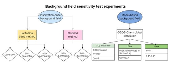
Figure 3. Background field sensitivity test experimental design framework.

Table 1. Names and specific parameters of five observation-based background fields.

Observation-Based Background Field	Name of Observation-Based Background Field	Statistical Method	Numerical Criteria for Filtering Background Fields
	Grid_50	Gridded method	50th percentile
	Grid_60	Gridded method	60th percentile
	Lati_30	Latitudinal band method	Lower 30th percentile
	Lati_60	Latitudinal band method	60th percentile
	Lati_80	Latitudinal band method	80th percentile

Note: Gridded method: Within a 7-day moving time window, the median or 60th percentile of all XCO₂ observations within a 2° grid radius around the target grid is used as the background concentration for that grid on a given day [55]. Latitudinal band method: For each 5° latitudinal band, within a 7-day moving time window, the 30th, 60th, or 80th percentile of all observations within the band represents the background concentration for all grids in that band on a given day.

Table 2. Names and specific parameters of five model-based background fields.

Model-Based Background Field	Name of Model-Based Background Field	Initial Field	Flux	Mask
	Reference	OCO-2 scaled	Prior A	1° × 1°
	CT2022_BG	CT2022	Prior A	1° × 1°
	CAMS_BG	Satellite-based CAMS	Prior A	1° × 1°
	GONGGA_BG	OCO-2 scaled	GONGGA posterior flux	1° × 1°
	Masktest_BG	OCO-2 scaled	Prior A	0.1° × 0.1°

In Section 2.3, two types of background fields are discussed: observation-based and model-based. Building on previous inversion studies that used observation-based background fields, we designed two categories comprising a total of five observation-based background fields (Table 1). The first category is the gridded background field (Gridded method in Table 1). Following the method of Feng et al. [55], we assume that within a 7-day moving time window, the median or 60th percentile of all XCO₂ observations within a 2$°$ grid radius around the target grid is used as the background concentration for that grid on a given day, and obtain the background fields Grid_50 and Grid_60. The second category is the latitudinal band background field (Latitudinal band method in Table 1), derived from the gridded background field. For each 5° latitudinal band, we assume that within a 7-day moving time window, the 30th, 60th, or 80th percentile of all observations within the band represents the background concentration for all grids in that band on a given day, and obtain the background fields Lati_30, Lati_60, and Lati_80. Using these configurations, we developed five observation-based background fields and conducted inversions to compare them with the model-based background fields. The results are detailed in Section 4.2.

Meantime, we designed five different model-based background fields to test the impact of various initial fields, carbon fluxes, and masks on the inversion results. The names and configurations of these five background fields are shown in Table 2. The background field used for the Results Section is referred to as the Reference background field (introduced in Section 2.3). Since initial fields have a greater impact on GEOS-Chem simulation results than flux distributions [37], we tested the effects of two other initial fields on the background field and results. These two initial fields are optimized CO₂ concentration fields obtained from previous inversion studies, specifically the CT2022 and CAMS v23r3 satellite products. In these two scenarios, we kept the flux field and mask consistent with the Reference background field for simulation and inversion. With these settings, we obtained two additional background fields based on different initial fields, named CT2022_BG and CAMS_BG.

Additionally, to evaluate the impact of different flux fields in GEOS-Chem on the background field and inversion results, we substituted the prior flux field used in this study with the posterior flux field optimized by the GONGGA system. Jin et al. provided the posterior flux fields derived from the GONGGA inversion system, which also assimilated OCO-2 observational data like ours, including fossil fuel, biomass burning, ocean, and terrestrial biospheric fluxes [41]. We used these four fluxes while keeping the initial field and mask consistent with the Reference background field, resulting in GONGGA_BG. Considering that the numerical diffusion characteristics of Eulerian models (e.g., GEOS-Chem) may introduce aggregation errors, we improved the spatial resolution of the mask to 0.1$° \times 0$.1$°$ to assess whether different spatial resolution masks affect the background field simulation and inversion results. The initial field and flux field of this background field are consistent with the Reference background field, resulting in Masktest_BG. The inversion results obtained from these five background fields are detailed in Section 4.2. The names and specific parameters of ten background fields are listed in Table 1 and Table 2.

3. Results

3.1. Evaluation for the Inversion Results

As outlined in Equation (1), the primary goal of MEGA is to optimize carbon fluxes by minimizing the discrepancy between model simulations and observations of XCO₂. To evaluate the inversion’s performance, we compared the column-averaged CO₂ concentration driven by the prior and posterior fluxes (referred to as prior and posterior XCO₂) derived from MEGA.

Figure 4a shows the bias (observed XCO₂ minus modeled XCO₂) and root mean square error (RMSE) of the prior and posterior XCO₂ simulations against OCO-2 XCO₂ observations from 2018 to 2023. The mean bias and RMSE for the prior XCO₂ concentrations compared to OCO-2 observations were 0.76 ppm and 1.3 ppm, respectively. With MEGA optimization, the posterior XCO₂ significantly reduced the mean bias and RMSE to 0.26 ppm and 0.95 ppm, respectively. The XCO₂ modeled using posterior fluxes demonstrated notable improvement over those based on prior fluxes.

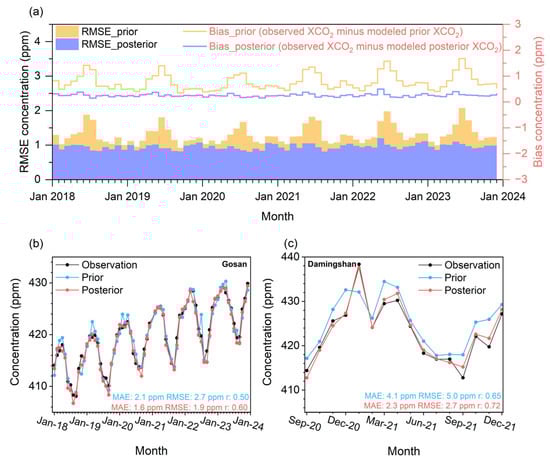
Figure 4. (a) Comparison of bias (observed XCO₂ minus simulated XCO₂) and root-mean-square error (RMSE) between monthly average OCO-2 XCO₂ and the monthly average prior and posterior XCO₂ simulated by MEGA from 2018–2023. The orange and blue lines indicate the biases for prior and posterior concentrations, while the orange and purple shaded areas depict the RMSE for prior and posterior data, respectively. Modeled and observed monthly mean CO₂ concentrations for China based on Gosan station (b) and Damingshan station (c). The available observation of Gosan station is from January 2018 to December 2023, and that of Damingshan station is from September 2020 to December 2021. The black line represents observations at each station, the red line shows the posterior concentration based on this study, and the blue line indicates the prior concentration from this study.

To independently evaluate the inversion performance over China, we utilized surface CO₂ observations from the Gosan station, located downwind of East Asia and proven to effectively capture CO₂ signals influenced by land carbon fluxes from China [48], and observations from the Damingshan station, a high-altitude station located in the most economically developed and densely forested regions in China [47].

Figure 4b compares the monthly averaged observed CO₂ concentrations at Gosan station with the prior and posterior CO₂ concentrations simulated by our MEGA-based inversion system. The posterior concentrations, optimized through MEGA-constrained land carbon fluxes, show significantly improved agreement with observations compared to the prior estimates. The correlation coefficient (r) increases from 0.50 (prior) to 0.60 (posterior), while the RMSE decreases by 30% from prior to posterior (from 2.7 ppm to 1.9 ppm) and the mean absolute error (MAE) decreases by 24% from prior to posterior (from 2.1 ppm to 1.6 ppm) during 2018–2023. Similarly, at Damingshan Station (Figure 4c), the posterior simulations exhibit robust enhancements: The mean correlation improves from 0.65 (prior) to 0.72 (posterior). The RMSE declines by 46% from prior to posterior (from 5.0 ppm to 2.7 ppm), and the MAE decreases by 44% from prior to posterior (from 4.1 ppm to 2.3 ppm). These statistically robust improvements demonstrate that the MEGA-based inversion system effectively enhances the accuracy of land carbon flux estimates over China.

MEGA-modeled XCO₂ concentration based on posterior fluxes closely matches the OCO-2 XCO₂ retrievals in both magnitude (bias = 0.25 ppm) and trend (r = 0.98), indicating that our flux estimate is effectively constrained by the assimilated OCO-2 XCO₂ retrievals (Figure S2). Spatial evaluation results showing the spatial distribution of correlations and biases between modeled and observed XCO₂ are provided in Figure S3. The posterior XCO₂ shows improved correlations and significantly reduced spatial biases compared to the prior across China, demonstrating the effectiveness of OCO-2 data assimilation in optimizing the spatial representation of XCO₂.

3.2. Regional Carbon Fluxes

Optimized by MEGA, our inversion results indicate that the mean annual terrestrial natural land fluxes (terrestrial biosphere flux plus fire flux) in China for 2018–2023 are −0.28 ± 0.15 PgC yr⁻¹. As shown in Figure 5a, we compiled inversion studies and national greenhouse gas inventories (NGHGIs) published in the past six years that estimated China’s carbon sink for 2018 and beyond. Despite the different time periods covered by each study, they consistently indicate that China’s ecosystem acted as a carbon sink during 2018–2023. Our estimates fall within the range of −0.44 to −0.16 PgC yr⁻¹ from previous estimates using various studies, with −0.16 PgC yr⁻¹ of CT2022 [11], −0.19 PgC yr⁻¹ of GCAS [56], −0.22 PgC yr⁻¹ of CAMS v24r1 (satellite) [51], −0.27 PgC yr⁻¹ of CAMS v23r3 (surface) [51], −0.32 ± 0.54 PgC yr⁻¹ of OCO-2 MIP [14], −0.34 PgC yr⁻¹ of Jena [57], −0.37 PgC yr⁻¹ of NGHGIs, −0.42 ± 0.15 PgC yr⁻¹ of GONGGA [41], and −0.44 PgC yr⁻¹ of Li et al. [13]. The methods of calculating annual flux uncertainty are detailed in the SI.

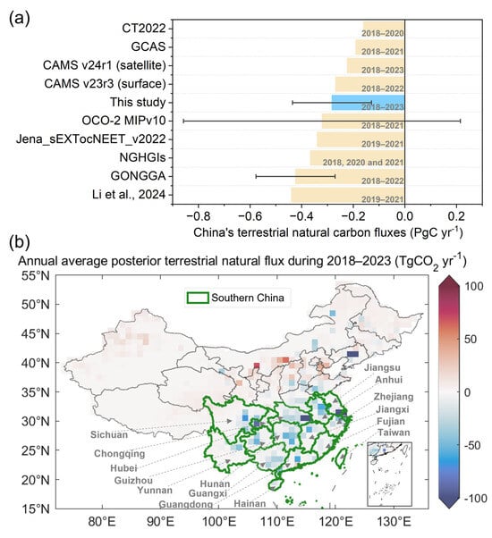
Figure 5. (a) Comparison of China’s terrestrial natural carbon fluxes (PgC yr⁻¹) from various studies, including Jena_sEXTocNEET_v2022 (average for 2019–2021) [57], CAMS v23r3-surface (average for 2018–2022) [51], CT2022 (average for 2018–2020) [11], Li et al. (average for 2019–2021) [13], GCAS (average for 2018–2021) [56], NGHGIs (2018) [58], OCO-2 MIPv10 (average for 2018–2021) [14], GONGGA (average for 2018–2022) [41], CAMS v23r3-satellite (average for 2018–2023) [51], and this study (average for 2018–2023). Error bars indicate the uncertainty range for each estimate. The blue bar represents the results from this study and the yellow bars represent the results from other studies. (b) Spatial distribution of China’s terrestrial natural carbon fluxes based on this study. Note that Southern China includes Jiangsu, Anhui, Zhejiang, Jiangxi, Fujian, Taiwan, Hainan, Hubei, Hunan, Guangdong, Guangxi, Sichuan, Chongqing, Guizhou, and Yunnan. The color scale represents the magnitude of carbon fluxes, with blue indicating carbon sinks and red indicating carbon sources. The area outlined in green represents Southern China, while the area not outlined in green represents outside Southern China.

As shown in Figure 5b, the average annual carbon sink (shown as negative values) in China from 2018 to 2023 is primarily located in Southern China, encompassing the provinces of Jiangsu, Anhui, Hubei, Sichuan, Chongqing, Zhejiang, Fujian, Taiwan, Hainan, Jiangxi, Hunan, Guizhou, Guangdong, Guangxi, and Yunnan. The terrestrial natural fluxes in Southern China are −0.47 ± 0.15 PgC yr⁻¹, indicating a net carbon sink. In contrast, areas outside Southern China act as a net carbon source, with fluxes of 0.19 ± 0.21 PgC yr⁻¹. Southern China contributes approximately 168% to China’s total carbon sink during 2018–2023, while terrestrial ecosystems outside this region offset 68% of Southern China’s carbon sink capacity.

We compared the terrestrial net carbon fluxes in Southern China and regions outside Southern China, where the net carbon flux in each area is calculated as the sum of terrestrial natural carbon fluxes and anthropogenic carbon emissions. Despite Southern China’s significantly higher carbon sink compared to regions outside, it does not achieve carbon neutrality during this period, with a net carbon flux of 0.63 ± 0.15 PgC yr⁻¹. This suggests that anthropogenic carbon emissions in Southern China exceed its carbon sink during 2018–2023, likely due to the area’s high population density and economic development.

3.3. Seasonal Cycle of Carbon Fluxes

As shown in Figure 6a, during the period from 2018 to 2023, China’s terrestrial natural ecosystems overall acted as a carbon source from January to April (with average terrestrial natural flux of 0.040 PgC month⁻¹), shifted to a carbon sink from May to September (with average terrestrial natural flux of −0.13 PgC month⁻¹), and reverted to a carbon source from October to December (with average terrestrial natural flux of 0.065 PgC month⁻¹). The seasonal cycles of terrestrial natural carbon flux estimated by MEGA across China are relatively consistent with those estimated by other studies (Figure 6a), with the peak carbon sink occurring in August (with average terrestrial natural flux of −0.19 PgC month⁻¹). We have gathered as many previous studies as possible that provide the seasonal cycles of terrestrial natural carbon flux in China for the period 2018–2023. The results from satellite-based CAMS, surface-based CAMS, and GONGGA are averages for 2018–2022, while CT2022 provides averages for 2018–2020, and OCO-2 MIP offers averages for 2018–2021.

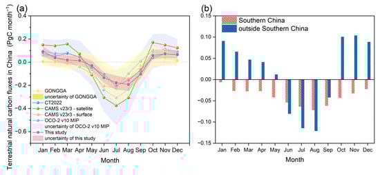
Figure 6. (a) Monthly average terrestrial natural carbon fluxes in China (PgC yr⁻¹) from January to December, comparing results from various studies including OCO-2 v10 MIP (average for 2018–2021) [14], GONGGA (average for 2018–2022) [41], CT2022 (average for 2018–2020) [11], CAMS v23r3-surface (average for 2018–2022) [51], CAMS v23r3-satellite (average for 2018–2023) [51], and this study. The purple, yellow, and pink shaded areas represent the uncertainty ranges for OCO-2 v10 MIP, GONGGA, and this study, respectively. (b) Monthly average terrestrial natural carbon fluxes from Southern China and regions outside Southern China during 2018–2023. The red bars indicate Southern China, while the blue bars represent areas outside Southern China.

When broken down into the monthly variations in terrestrial natural carbon flux distribution, we focus on identifying which region predominantly influences the shift between carbon source and sink roles in China’s terrestrial natural ecosystems across different seasons. According to Figure 6b, from 2018 to 2023, the terrestrial natural ecosystems in southern China consistently acted as a carbon sink throughout the year, showing no seasonal variation. In contrast, the ecosystems outside Southern China served as a carbon sink from June to September, aligning with the plant growing season, and acted as a carbon source during other months, exhibiting seasonal variation.

The seasonal variation in carbon fluxes of terrestrial natural ecosystems outside Southern China primarily drives the shift in carbon source and sink roles of China’s overall terrestrial natural ecosystems across different seasons. From January to April, the carbon source effect outside Southern China (average terrestrial natural carbon flux of 0.061 PgC month⁻¹) significantly outweighed the carbon sink effect in southern China (average terrestrial natural carbon flux of −0.020 PgC month⁻¹), making China’s terrestrial natural ecosystems a carbon source during this period. In May, the terrestrial natural carbon flux outside Southern China decreased by 0.029 PgC compared to April, reaching 0.012 PgC month⁻¹, while the carbon sink effect in southern China became dominant, turning China’s overall terrestrial natural ecosystems from a carbon source to a carbon sink. From June to September, both southern and outside Southern China had negative terrestrial natural carbon fluxes (−0.063 PgC month⁻¹ and −0.089 PgC month⁻¹, respectively). From October to December, the terrestrial natural carbon flux outside Southern China rapidly increased to 0.098 PgC month⁻¹, causing the ecosystems in this area to shift from being a carbon sink to a carbon source. This value significantly exceeds the carbon sink effect in southern China (terrestrial natural carbon flux of −0.033 PgC month⁻¹), thereby leading to the overall transformation of China’s terrestrial natural ecosystems into a carbon source.

4. Discussion

4.1. Influence of Prior Fluxes and Uncertainties

Here, we present the effects of different sets of prior scaling factors (introduced in Section 2.6.1), prior flux uncertainties, and prior fluxes on terrestrial net carbon fluxes (see Figure 7a,b). First, we conducted six sets of sensitivity tests of scaling the prior and prior uncertainty under the same prior using Prior C (Figure 7a). Whether we scaled the prior flux to 0.5× or 1.5×, or scaled the prior uncertainty to 50% or 200%, the posterior results converged within a relatively consistent range, with a mean relative deviation of 5.1% across the six sets of prior uncertainty results. Additionally, as shown in Figure 7b, under the same prior scaling factor (1×) and prior uncertainty (50%), the posterior terrestrial net carbon fluxes obtained using three different prior emission fields (Prior A, Prior B, and Prior C) were also relatively consistent, with a mean relative deviation of 3.2% between the results. Even when assuming a constant prior each month (Prior C), we still obtained posterior results that reflect the seasonal variation in China’s carbon sink. The posterior results based on Prior C were found to be highly consistent with the posterior results obtained using monthly varying priors (Prior A and Prior B), with correlation coefficients of 0.99 for both comparisons. This indicates that the inversion results of this assimilation system are well-constrained by observations and are robust. The effects of prior scaling factor, prior uncertainty, and different priors on terrestrial natural carbon fluxes are detailed in Figures S3 and S4 of the SI, consistent with the above conclusions.

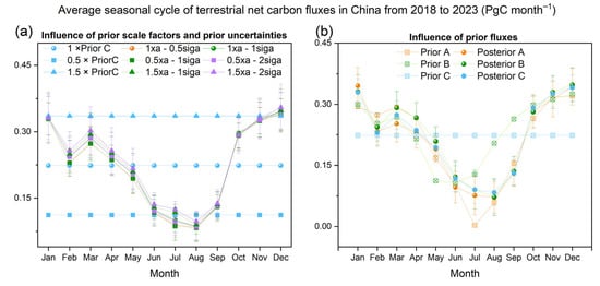
Figure 7. Average seasonal cycle of terrestrial net carbon fluxes in China from 2018 to 2023, illustrating the influence of various factors. (a) Impact of prior scale factors and uncertainties, showing different scenarios such as 1×, 0.5×, and 1.5× Prior C with varying sigma levels. (b) Influence of prior fluxes, comparing different prior and posterior scenarios (A, B, C).

4.2. Influence of Background Fields and Uncertainties

In this study, we tested the impact of 10 different background fields on the inversion results of the year 2018. During the background field testing phase, we used the controlled variable method to ensure that all inversion parameters, except for the background field, remained consistent, including the use of Prior A, 1× prior uncertainty, and 50% prior uncertainty. As mentioned in Section 2.6.2, we tested 5 observation-based and 5 model-based background fields. We primarily evaluated the simulation effects of the inversion results based on different background fields according to indicators (correlation, standard deviation, and root mean square error between posterior, prior, and observed concentrations) and the seasonal cycle of terrestrial natural carbon fluxes obtained under different background fields. Previous studies have compared the impacts of model-based versus observation-based background fields on ground-based observation assimilation inversions [26], whereas this study represents the first comprehensive comparison of their effects on satellite observation assimilation inversions.

The correlation (r) (Figure 8a) and root mean square error (RMSE) (Figure 8b) between the posterior and observed XCO₂ obtained from the 11 background fields (mean r and RMSE of 0.90 and 0.97 ppm, respectively) were superior to those between the prior and observed XCO₂ (mean r and RMSE of 0.84 and 1.42 ppm, respectively). Except for the two gridded background fields (grid_50, grid_60), the posterior XCO₂ obtained from the other 8 background fields reduced the mean bias from 0.68 ppm (bias of prior concentration) to 0.19 ppm. The posterior concentrations obtained from the two gridded background fields, however, increased the bias from −0.073 ppm to 0.12 ppm (Figure 8c). We found that relying solely on the above statistical indicators is insufficient to select the optimal background field.

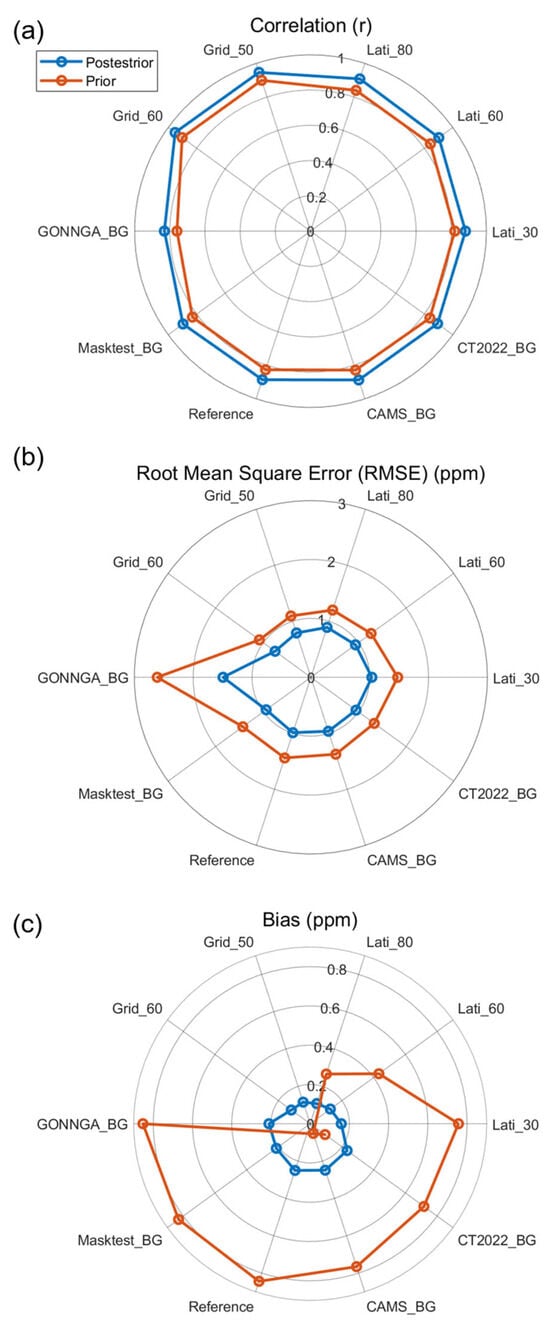
Figure 8. Evaluation of model performance using different background fields. (a) Correlation (r) between posterior and prior estimates across various background configurations. (b) Root Mean Square Error (RMSE) in ppm, comparing posterior and prior results for each background field. (c) Bias in ppm, illustrating differences between posterior and prior estimates. Blue lines represent posterior results, while orange lines indicate prior results.

By examining the seasonal cycle of terrestrial natural carbon fluxes, we found that the five observation-based background fields failed to accurately represent the seasonal variation characteristics of China’s terrestrial carbon sinks (Figure 9a). Figure 9a shows the results obtained from inversions based on 5 observation-based background fields, as well as the seasonal cycle of China’s terrestrial natural carbon fluxes in 2018 from previous studies. The inversion results based on 5 observation-based background fields did not exhibit consistent amplitudes (peak-to-trough differences in the seasonal natural land flux cycle) or phases (source-to-sink transitions) with these previous studies. The inversion results of terrestrial natural carbon fluxes using gridded background fields exhibited a relatively small amplitude (0.10–0.11 PgC), with negative values persisting throughout the year and no positive phase observed, suggesting that this approach failed to capture significant seasonal fluctuations. In contrast, inversions based on latitude band background fields (e.g., Lati_30, Lati_60, and Lati_90) showed amplitudes ranging from 0.21 to 0.26 PgC, which were significantly higher than those derived from the gridded method. However, these values remained lower than the higher amplitude range (0.28–0.54 PgC) reported in previous studies. And the changes in inversions based on latitude band background fields observed in July and August were contrary to those reported in previous studies, showing a decrease in carbon sinks instead of an increase, which is inconsistent with the recognized seasonal variation characteristics of China’s carbon sink.

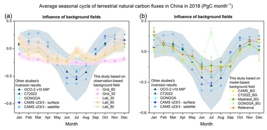
Figure 9. Average seasonal cycle of terrestrial natural carbon fluxes in China in 2018, illustrating the influence of various factors. (a) Influence of observation-based background fields, comparing results from this study with other inversion results. (b) Influence of model-based background fields, highlighting the impact of initial fields, flux fields, and mask. The shaded areas represent the range of other studies’ inversion results and their uncertainties.

We found that model-based background fields could effectively capture the seasonal fluctuations in terrestrial natural carbon fluxes, and among them, the Reference background field used in this study is currently the optimal background field. Figure 9b shows the results obtained from inversions based on five model-based background fields, as well as the seasonal cycle of China’s terrestrial natural carbon fluxes in 2018 from previous studies. These tests covered the effects of different initial concentration fields, flux fields, and masks (introduced in Section 2.6.2) on the results. It can be seen that, except for the inversion results based on GONGGA flux fields (GONGGA_BG), the other 9 background fields exhibit some seasonal variation characteristics. However, during the peak growing season in July and August, not all background fields show the strongest carbon sink. By comparing the terrestrial natural carbon fluxes from the inversions using the reference scenario, CT2022_BG scenario, and CAMS_BG scenario (introduced in Section 2.6.2 and Table 1) (Figure 9b), we can conclude that only our Reference background field-based inversion shows the strongest carbon sink in July and August, agreeing with other studies.

Furthermore, we found that background fields simulated using different initial fields mainly affect the estimation of terrestrial natural carbon fluxes in January–February, June–August, and October–December. When using different initial fields, monthly absolute deviation of posterior terrestrial natural carbon fluxes based on CT2022_BG and CAMS_BG relative to those based on Reference background field is 0.11, 0.052, and 0.053 PgC month⁻¹ for January–February, June–August, and October–December, respectively, while for other months (March–May and September), this value is 0.0087 PgC month⁻¹. Background fields estimated using different flux fields mainly affect the estimation of terrestrial natural carbon fluxes in June–August, with posterior results based on GONGGA_BG showing a deviation of 0.18 PgC month⁻¹ relative to those based on the Reference background field, while for January–May and September–December, these values are 0.041 and 0.030 PgC month⁻¹, respectively.

Additionally, we found that GEOS-Chem simulations indeed have some aggregation errors, consistent with the views of Rigby et al. [22]. As illustrated in Figure 9b, the monthly terrestrial natural carbon flux calculated using the 0.1° × 0.1° mask (Masktest_BG) exhibited a mean reduction of 0.0067 Pg C month⁻¹ relative to the posterior estimates derived from the 1° × 1° mask (Reference). This means that the GEOS-Chem simulation, when using a 0.1$° \times 0$.1$°$ mask to turn off emissions within China, may misidentify grids that should belong to China as non-China grids due to aggregation errors, leaving some grid emissions unturned off. This ultimately leads to an overestimation of the background field and an underestimation of terrestrial natural carbon flux when simulating the background field based on a 0.1$° \times 0$.1$°$ mask.

4.3. Limitations and Future Perspectives

In the prior sensitivity test, we demonstrated that the posterior terrestrial natural carbon fluxes for China estimated by the MEGA inversion system are numerically and seasonally robust. This indicates that MEGA is not sensitive to the choice of prior fluxes. This study performed sensitivity tests on up to 10 background fields, but did not explore all possible simulations, primarily due to constraints in selecting initial fields. There were some studies that have optimized global carbon flux fields using various global inversion systems; however, few have publicly released optimized global 3D concentration fields, except for CT2022 and CAMS.

The MEGA system combines OCO-2 observations (to calibrate initial fields) with GEOS-Chem model simulations (to capture background transport and seasonal variations), forming a hybrid approach for background field construction. Our sensitivity tests (Section 4.2) demonstrate that this hybrid method effectively captures seasonal flux dynamics, particularly during peak growing seasons. However, the current background field simulation approach still has limitations, as evidenced by the sensitivity of inversion results to different initial fields, flux fields, and mask resolutions. Future work should continue to refine background field simulations to reduce uncertainties in regional carbon sink estimates at their source.

Another important source of uncertainty lies in anthropogenic fossil fuel emission inventories. In the MEGA system, terrestrial natural carbon fluxes are derived as residuals by subtracting prescribed fossil fuel emissions from the optimized net carbon flux. Uncertainties in fossil fuel emission inventories thus propagate directly into biospheric flux estimates, potentially obscuring the true biospheric signal. This effect is most pronounced in densely urbanized and industrialized regions such as southeastern China, where small relative errors in fossil fuel emission estimates can translate into significant absolute errors in biospheric flux retrievals. Different emission inventories (e.g., ODIAC, EDGAR) may yield substantially different biospheric flux estimates. Future work should explore the sensitivity of biospheric flux estimates to different fossil fuel emission inventories and consider jointly optimizing both biospheric and fossil fuel emissions within the inversion systems.

The MEGA inversion system is well-suited for long-lived trace greenhouse gases, such as CO₂ and CH₄. By integrating the strengths of Lagrangian and Eulerian models, it allows the source–receptor relationship from a single Lagrangian model run to be applied to multiple gases, thereby reducing the cost of multi-species inversions. Moreover, MEGA is versatile and can be applied to any region. This study uses China as a case study to demonstrate the principles, setup, and results of MEGA. In the future, we plan to explore MEGA’s inversion capabilities in other countries, including small developed nations (e.g., Japan, South Korea), tropical countries (e.g., Indonesia), and polar regions (e.g., Russia).

5. Conclusions

This study developed and applied the Monitoring and Evaluation of Greenhouse gAs Flux (MEGA) inversion system—a Lagrangian–Eulerian combined model framework specifically optimized for satellite observation assimilation. While existing combined Eulerian–Lagrangian frameworks have primarily been developed and optimized for ground-based observation networks, MEGA addresses the distinct characteristics and challenges of satellite observations. By combining Lagrangian models’ high-resolution capability (1° × 1°) with Eulerian models, MEGA enables regional inversions at finer spatial scales than typical global Eulerian systems (4° × 5°). This approach to satellite data assimilation offers significant potential for reducing uncertainties in regional carbon sink estimates.

Using China as a case study, we utilized this regional inversion system to derive monthly gridded carbon fluxes from OCO-2 XCO₂ V11.1r data. We examined their magnitudes and variations to gain insights into China’s terrestrial carbon fluxes from 2018 to 2023. Firstly, compared with the OCO-2 XCO₂ retrievals, mean bias and RMSE decrease from prior values of 0.76 and 1.3 ppm to 0.26 and 0.95 ppm, respectively, indicating that the MEGA works well with the OCO-2 XCO₂ retrievals. Furthermore, independent evaluations using surface observation showed that the posterior carbon fluxes could significantly improve the modeling of atmospheric CO₂ concentrations. Our estimates of China’s carbon flux inversion were generally consistent with the ensemble results from multiple inversion systems in the OCO-2 MIP and other studies, both in terms of annual and seasonal variations. In the regional analysis, we found that southern China (including Jiangsu, Anhui, Hubei, Sichuan, Chongqing, Zhejiang, Fujian, Taiwan, Hainan, Jiangxi, Hunan, Guizhou, Guangdong, Guangxi, and Yunnan provinces) acted as a continuous carbon sink throughout the year over the six-year average from 2018 to 2023, making it the largest contributor to China’s carbon sink. In contrast, the terrestrial natural carbon fluxes in remaining regions of China exhibited significant seasonal sinks in the growing season and sources in the nongrowing season, dominating the overall seasonal changes in China’s terrestrial natural carbon fluxes.

We further investigated the robustness and uncertainties of our inversion results in relation to the choices of prior fluxes and background field. The prior sensitivity tests varied in terms of the utilized prior fluxes, prior scaling factor, and prior uncertainty. Results from six sets of prior sensitivity tests indicated that the inversion results under the MEGA system were very robust and insensitive to the aforementioned prior parameters. This study provides the first comprehensive assessment of how different background approaches (model-based versus observation-based) influence satellite observation assimilation inversion. The background field sensitivity tests included a total of 10 sets of results. We first compared the performance of observation-based background fields and model-based background fields in MEGA. We found that the five different observation-based background fields failed to capture the seasonal variation characteristics of China’s terrestrial natural carbon fluxes, possibly because observation-based background fields do not cover the impact of meteorology and other factors. In contrast, model-based background fields consider multiple factors such as emissions, meteorology, and observations, better reflecting the seasonal disturbances of terrestrial natural carbon fluxes caused by these factors. Therefore, compared to observation-based background fields, model-based background fields performed better in revealing the seasonal variations in China’s terrestrial natural carbon fluxes. Similarly, we explored the impact of initial fields, flux fields, and masks (used to control regional flux switches) on model-based background fields and their corresponding inversion results. By comparing inversion results derived from five different model-based background fields, we found that the Reference background field represented the optimal configuration in the current inversion framework. Meanwhile, initial fields, flux fields, and masks all had varying degrees of impact on model-based background fields and their inversion results. While previous research has rigorously examined the differential impacts of model-derived and observation-constrained background fields within ground-based data assimilation frameworks, our work addresses this critical gap by conducting the first systematic analysis of their divergent influences on satellite-based assimilation inversions, thereby advancing our understanding of background field dependency in multi-platform observational systems.

The sensitivity inversion evaluations, along with comparisons to previous inversion models and data products, underscore the committed future development path of our atmospheric inversion system, reflecting a sustained and ongoing endeavor.

References

- WMO. WMO Greenhouse Gas Bulletin No.20; WMO: Geneva, Switzerland, 2024; p. 1. [Google Scholar]
- IPCC. Climate Change 2023: Synthesis Report. Contribution of Working Groups I, II and III to the Sixth Assessment Report of the Intergovernmental Panel on Climate Change; Core Writing Team, Lee, H., Romero, J., Eds.; Cambridge University Press: Cambridge, UK, 2023; 184p. [Google Scholar]
- Gurney, K.R.; Law, R.M.; Denning, A.S.; Rayner, P.J.; Baker, D.; Bousquet, P.; Bruhwiler, L.; Chen, Y.-H.; Ciais, P.; Fan, S.; et al. Towards robust regional estimates of CO2 sources and sinks using atmospheric transport models. Nature 2002, 415, 626–630. [Google Scholar] [CrossRef]
- Ciais, P.; Rayner, P.; Chevallier, F.; Bousquet, P.; Logan, M.; Peylin, P.; Ramonet, M. Atmospheric inversions for estimating CO2 fluxes: Methods and perspectives. Climatic Change 2010, 103, 69–92. [Google Scholar] [CrossRef]
- Peiro, H.; Crowell, S.; Schuh, A.; Baker, D.F.; O’Dell, C.; Jacobson, A.R.; Chevallier, F.; Liu, J.J.; Eldering, A.; Crisp, D.; et al. Four years of global carbon cycle observed from the Orbiting Carbon Observatory 2 (OCO-2) version 9 and in situ data and comparison to OCO-2 version 7. Atmos. Chem. Phys. 2022, 22, 1097–1130. [Google Scholar] [CrossRef]
- Baker, D.F.; Law, R.M.; Gurney, K.R.; Rayner, P.; Peylin, P.; Denning, A.S.; Bousquet, P.; Bruhwiler, L.; Chen, Y.H.; Ciais, P.; et al. TransCom 3 inversion intercomparison: Impact of transport model errors on the interannual variability of regional CO fluxes, 1988–2003. Glob. Biogeochem. Cycles 2006, 20. [Google Scholar] [CrossRef]
- Peylin, P.; Law, R.M.; Gurney, K.R.; Chevallier, F.; Jacobson, A.R.; Maki, T.; Niwa, Y.; Patra, P.K.; Peters, W.; Rayner, P.J.; et al. Global atmospheric carbon budget: Results from an ensemble of atmospheric CO inversions. Biogeosciences 2013, 10, 6699–6720. [Google Scholar] [CrossRef]
- Houweling, S.; Baker, D.; Basu, S.; Boesch, H.; Butz, A.; Chevallier, F.; Deng, F.; Dlugokencky, E.J.; Feng, L.; Ganshin, A.; et al. An intercomparison of inverse models for estimating sources and sinks of CO using GOSAT measurements. J. Geophys. Res. Atmos. 2015, 120, 5253–5266. [Google Scholar] [CrossRef]
- Zhang, L.; Jiang, F.; He, W.; Wu, M.; Wang, J.; Ju, W.; Wang, H.; Zhang, Y.; Sitch, S.; Chen, J.M. Improved estimates of net ecosystem exchanges in mega-countries using GOSAT and OCO-2 observations. Commun. Earth Environ. 2024, 5, 737. [Google Scholar] [CrossRef]
- Villalobos, Y.; Rayner, P.J.; Silver, J.D.; Thomas, S.; Haverd, V.; Knauer, J.; Loh, Z.M.; Deutscher, N.M.; Griffith, D.W.T.; Pollard, D.F. Was Australia a sink or source of CO2 in 2015? Data assimilation using OCO-2 satellite measurements. Atmos. Chem. Phys. 2021, 21, 17453–17494. [Google Scholar] [CrossRef]
- Jacobson, A.R.; Schuldt, K.N.; Tans, P.; Arlyn, A.; Miller, J.B.; Oda, T.; Mund, J.; Weir, B.; Ott, L.; Aalto, T.; et al. CarbonTracker CT2022; NOAA Global Monitoring Laboratory: Boulder, CO, USA, 2023. [Google Scholar]
- Wang, J.; Feng, L.; Palmer, P.I.; Liu, Y.; Fang, S.; Bösch, H.; O’Dell, C.W.; Tang, X.; Yang, D.; Liu, L.; et al. Large Chinese land carbon sink estimated from atmospheric carbon dioxide data. Nature 2020, 586, 720–723. [Google Scholar] [CrossRef]
- Li, J.; Zhang, X.; Guo, L.; Zhong, J.; Wang, D.; Wu, C.; Li, F.; Li, M. Invert global and China’s terrestrial carbon fluxes over 2019–2021 based on assimilating richer atmospheric CO2 observations. Sci. Total Environ. 2024, 929, 172320. [Google Scholar] [CrossRef]
- Byrne, B.; Baker, D.F.; Basu, S.; Bertolacci, M.; Bowman, K.W.; Carroll, D.; Chatterjee, A.; Chevallier, F.; Ciais, P.; Cressie, N.; et al. National CO2 budgets (2015–2020) inferred from atmospheric CO2 observations in support of the global stocktake. Earth Syst. Sci. Data 2023, 15, 963–1004. [Google Scholar] [CrossRef]
- Stohl, A.; Seibert, P.; Arduini, J.; Eckhardt, S.; Fraser, P.; Greally, B.R.; Lunder, C.; Maione, M.; Mühle, J.; O’Doherty, S.; et al. An analytical inversion method for determining regional and global emissions of greenhouse gases: Sensitivity studies and application to halocarbons. Atmos. Chem. Phys. 2009, 9, 1597–1620. [Google Scholar] [CrossRef]
- Manning, A.J.; O’Doherty, S.; Jones, A.R.; Simmonds, P.G.; Derwent, R.G. Estimating UK methane and nitrous oxide emissions from 1990 to 2007 using an inversion modeling approach. J. Geophys. Res. Atmos. 2011, 116. [Google Scholar] [CrossRef]
- Vojta, M.; Plach, A.; Annadate, S.; Park, S.; Lee, G.; Purohit, P.; Lindl, F.; Lan, X.; Mühle, J.; Thompson, R.L.; et al. A global re-analysis of regionally resolved emissions and atmospheric mole fractions of SF6 for the period 2005–2021. Atmos. Chem. Phys. 2024, 24, 12465–12493. [Google Scholar] [CrossRef]
- Ganshin, A.; Oda, T.; Saito, M.; Maksyutov, S.; Valsala, V.; Andres, R.J.; Fisher, R.E.; Lowry, D.; Lukyanov, A.; Matsueda, H.; et al. A global coupled Eulerian-Lagrangian model and 1 × 1 km CO2 surface flux dataset for high-resolution atmospheric CO2 transport simulations. Geosci. Model Dev. 2012, 5, 231–243. [Google Scholar] [CrossRef]
- Koyama, Y.; Maksyutov, S.; Mukai, H.; Thoning, K.; Tans, P. Simulation of variability in atmospheric carbon dioxide using a global coupled Eulerian–Lagrangian transport model. Geosci. Model Dev. 2011, 4, 317–324. [Google Scholar] [CrossRef]
- Vermeulen, A.T.; Pieterse, G.; Hensen, A.; van den Bulk, W.C.M.; Erisman, J.W. COMET: A Lagrangian transport model for greenhouse gas emission estimation–forward model technique and performance for methane. Atmos. Chem. Phys. Discuss. 2006, 2006, 8727–8779. [Google Scholar] [CrossRef]
- Trusilova, K.; Rödenbeck, C.; Gerbig, C.; Heimann, M. Technical Note: A new coupled system for global-to-regional downscaling of CO2 concentration estimation. Atmos. Chem. Phys. 2010, 10, 3205–3213. [Google Scholar] [CrossRef]
- Rigby, M.; Manning, A.J.; Prinn, R.G. Inversion of long-lived trace gas emissions using combined Eulerian and Lagrangian chemical transport models. Atmos. Chem. Phys. 2011, 11, 9887–9898. [Google Scholar] [CrossRef]
- Stohl, A.; Kim, J.; Li, S.; O’Doherty, S.; Mühle, J.; Salameh, P.K.; Saito, T.; Vollmer, M.K.; Wan, D.; Weiss, R.F.; et al. Hydrochlorofluorocarbon and hydrofluorocarbon emissions in East Asia determined by inverse modeling. Atmos. Chem. Phys. 2010, 10, 3545–3560. [Google Scholar] [CrossRef]
- He, W.; Jiang, F.; Ju, W.; Chevallier, F.; Baker, D.F.; Wang, J.; Wu, M.; Johnson, M.S.; Philip, S.; Wang, H.; et al. Improved Constraints on the Recent Terrestrial Carbon Sink Over China by Assimilating OCO-2 XCO2 Retrievals. J. Geophys. Res. Atmos. 2023, 128, e2022JD037773. [Google Scholar] [CrossRef]
- Tarantola, A. Inverse Problem Theory and Methods for Model Parameter Estimation; Society for Industrial and Applied Mathematics: Philadelphia, PA, USA, 2005. [Google Scholar]
- Vojta, M.; Plach, A.; Thompson, R.L.; Stohl, A. A comprehensive evaluation of the use of Lagrangian particle dispersion models for inverse modeling of greenhouse gas emissions. Geosci. Model Dev. 2022, 15, 8295–8323. [Google Scholar] [CrossRef]
- Vollmer, M.K.; Zhou, L.X.; Greally, B.R.; Henne, S.; Yao, B.; Reimann, S.; Stordal, F.; Cunnold, D.M.; Zhang, X.C.; Maione, M.; et al. Emissions of ozone-depleting halocarbons from China. Geophys. Res. Lett. 2009, 36. [Google Scholar] [CrossRef]
- Seibert, P.; Frank, A. Source-receptor matrix calculation with a Lagrangian particle dispersion model in backward mode. Atmos. Chem. Phys. 2004, 4, 51–63. [Google Scholar] [CrossRef]
- Rigby, M.; Park, S.; Saito, T.; Western, L.M.; Redington, A.L.; Fang, X.; Henne, S.; Manning, A.J.; Prinn, R.G.; Dutton, G.S.; et al. Increase in CFC-11 emissions from eastern China based on atmospheric observations. Nature 2019, 569, 546–550. [Google Scholar] [CrossRef]
- Maksyutov, S.; Oda, T.; Saito, M.; Janardanan, R.; Belikov, D.; Kaiser, J.W.; Zhuravlev, R.; Ganshin, A.; Valsala, V.K.; Andrews, A.; et al. Technical note: A high-resolution inverse modelling technique for estimating surface CO2 fluxes based on the NIES-TM–FLEXPART coupled transport model and its adjoint. Atmos. Chem. Phys. 2021, 21, 1245–1266. [Google Scholar] [CrossRef]
- Bergamaschi, P.; Segers, A.; Brunner, D.; Haussaire, J.M.; Henne, S.; Ramonet, M.; Arnold, T.; Biermann, T.; Chen, H.; Conil, S.; et al. High-resolution inverse modelling of European CH4 emissions using the novel FLEXPART-COSMO TM5 4DVAR inverse modelling system. Atmos. Chem. Phys. 2022, 22, 13243–13268. [Google Scholar] [CrossRef]
- Sijikumar, S.; Raju, A.; Valsala, V.; Tiwari, Y.; Girach, I.A.; Jain, C.D.; Ratnam, M.V. High-Resolution Bayesian Inversion of Carbon Dioxide Flux Over Peninsular India. Atmos. Environ. 2023, 308, 119868. [Google Scholar] [CrossRef]
- He, C.; Lu, X.; Zhang, Y.; Liu, Z.; Jiang, F.; Sun, Y.; Gao, M.; Liu, Y.; Lin, H.; Yang, J.; et al. Revisiting the quantification of power plant CO2 emissions in the United States and China from satellite: A comparative study using three top-down approaches. Remote Sens. Environ. 2024, 308, 114192. [Google Scholar] [CrossRef]
- Li, B.; Huang, J.; Hu, X.; Zhang, L.; Ma, M.; Hu, L.; Chen, D.; Du, Q.; Sun, Y.; Cai, Z.; et al. CCl4 emissions in eastern China during 2021–2022 and exploration of potential new sources. Nat. Commun. 2024, 15, 1725. [Google Scholar] [CrossRef]
- Sun, Y.; Yao, B.; Ma, M.; Hu, X.; Ji, M.; Fang, X. Emissions of HCFC-22 and HCFC-142b in China during 2018–2021 Inferred from Inverse Modeling. Environ. Sci. Technol. 2024, 58, 13273–13283. [Google Scholar] [CrossRef]
- Bakels, L.; Tatsii, D.; Tipka, A.; Thompson, R.; Dütsch, M.; Blaschek, M.; Seibert, P.; Baier, K.; Bucci, S.; Cassiani, M.; et al. FLEXPART version 11: Improved accuracy, efficiency, and flexibility. Geosci. Model Dev. 2024, 17, 7595–7627. [Google Scholar] [CrossRef]
- Nassar, R.; Jones, D.B.A.; Suntharalingam, P.; Chen, J.M.; Andres, R.J.; Wecht, K.J.; Yantosca, R.M.; Kulawik, S.S.; Bowman, K.W.; Worden, J.R.; et al. Modeling global atmospheric CO2 with improved emission inventories and CO2 production from the oxidation of other carbon species. Geosci. Model Dev. 2010, 3, 689–716. [Google Scholar] [CrossRef]
- Bey, I.; Jacob, D.J.; Yantosca, R.M.; Logan, J.A.; Field, B.D.; Fiore, A.M.; Li, Q.; Liu, H.Y.; Mickley, L.J.; Schultz, M.G. Global modeling of tropospheric chemistry with assimilated meteorology: Model description and evaluation. J. Geophys. Res. Atmos. 2001, 106, 23073–23095. [Google Scholar] [CrossRef]
- Feng, L.; Palmer, P.I.; Bösch, H.; Dance, S. Estimating surface CO2 fluxes from space-borne CO2 dry air mole fraction observations using an ensemble Kalman Filter. Atmos. Chem. Phys. 2009, 9, 2619–2633. [Google Scholar] [CrossRef]
- Deng, F.; Jones, D.B.A.; Henze, D.K.; Bousserez, N.; Bowman, K.W.; Fisher, J.B.; Nassar, R.; O’Dell, C.; Wunch, D.; Wennberg, P.O.; et al. Inferring regional sources and sinks of atmospheric CO2 from GOSAT XCO2 data. Atmos. Chem. Phys. 2014, 14, 3703–3727. [Google Scholar] [CrossRef]
- Jin, Z.; Tian, X.; Wang, Y.; Zhang, H.; Zhao, M.; Wang, T.; Ding, J.; Piao, S. A global surface CO2 flux dataset (2015–2022) inferred from OCO-2 retrievals using the GONGGA inversion system. Earth Syst. Sci. Data 2024, 16, 2857–2876. [Google Scholar] [CrossRef]
- Kong, Y.; Zheng, B.; Zhang, Q.; He, K. Global and regional carbon budget for 2015–2020 inferred from OCO-2 based on an ensemble Kalman filter coupled with GEOS-Chem. Atmos. Chem. Phys. 2022, 22, 10769–10788. [Google Scholar] [CrossRef]
- Oda, T.; Maksyutov, S. ODIAC Fossil Fuel CO2 Emissions Dataset, version ODIAC2023; Center for Global Environmental Research: Tsukuba, Japan, 2015. [Google Scholar]
- van Wees, D.; van der Werf, G.R.; Randerson, J.T.; Rogers, B.M.; Chen, Y.; Veraverbeke, S.; Giglio, L.; Morton, D.C. Global biomass burning fuel consumption and emissions at 500 m spatial resolution based on the Global Fire Emissions Database (GFED). Geosci. Model. Dev. 2022, 15, 8411–8437. [Google Scholar] [CrossRef]
- Haynes, K.D.; Baker, I.T.; Denning, A.S. SiB4 Modeled Global 0.5-Degree Hourly Carbon Fluxes and Productivity, 2000-2018; ORNL Distributed Active Archive Center: Oak Ridge, TN, USA, 2021. [Google Scholar]
- Crisp, D.; Pollock, H.R.; Rosenberg, R.; Chapsky, L.; Lee, R.A.M.; Oyafuso, F.A.; Frankenberg, C.; O’Dell, C.W.; Bruegge, C.J.; Doran, G.B.; et al. The on-orbit performance of the Orbiting Carbon Observatory-2 (OCO-2) instrument and its radiometrically calibrated products. Atmos. Meas. Tech. 2017, 10, 59–81. [Google Scholar] [CrossRef]
- Chen, Y.; Lu, Y.; Qi, B.; Ma, Q.; Zang, K.; Lin, Y.; Liu, S.; Pan, F.; Li, S.; Guo, P.; et al. Atmospheric CO2 in the megacity Hangzhou, China: Urban-suburban differences, sources and impact factors. Sci. Total Environ. 2024, 926, 171635. [Google Scholar] [CrossRef] [PubMed]
- Kim, J.; Li, S.; Mühle, J.; Stohl, A.; Kim, S.-K.; Park, S.; Park, M.-K.; Weiss, R.F.; Kim, K.-R. Overview of the findings from measurements of halogenated compounds at Gosan (Jeju Island, Korea) quantifying emissions in East Asia. J. Integr. Environ. Sci. 2012, 9 (Suppl. 1), 71–80. [Google Scholar] [CrossRef]
- Park, S.; Western, L.M.; Saito, T.; Redington, A.L.; Henne, S.; Fang, X.; Prinn, R.G.; Manning, A.J.; Montzka, S.A.; Fraser, P.J.; et al. A decline in emissions of CFC-11 and related chemicals from eastern China. Nature 2021, 590, 433–437. [Google Scholar] [CrossRef]
- Zhou, L.; White, J.W.C.; Conway, T.J.; Mukai, H.; MacClune, K.; Zhang, X.; Wen, Y.; Li, J. Long-term record of atmospheric CO2 and stable isotopic ratios at Waliguan Observatory: Seasonally averaged 1991–2002 source/sink signals, and a comparison of 1998–2002 record to the 11 selected sites in the Northern Hemisphere. Global Biogeochem. Cycles 2006, 20. [Google Scholar] [CrossRef]
- Chevallier, F.; Remaud, M.; O’Dell, C.W.; Baker, D.; Peylin, P.; Cozic, A. Objective evaluation of surface- and satellite-driven carbon dioxide atmospheric inversions. Atmos. Chem. Phys. 2019, 19, 14233–14251. [Google Scholar] [CrossRef]
- Chevallier, F.; Ciais, P.; Conway, T.J.; Aalto, T.; Anderson, B.E.; Bousquet, P.; Brunke, E.G.; Ciattaglia, L.; Esaki, Y.; Fröhlich, M.; et al. CO2 surface fluxes at grid point scale estimated from a global 21 year reanalysis of atmospheric measurements. J. Geophys. Res. Atmos. 2010, 115. [Google Scholar] [CrossRef]
- Crowell, S.; Baker, D.; Schuh, A.; Basu, S.; Jacobson, A.R.; Chevallier, F.; Liu, J.; Deng, F.; Feng, L.; McKain, K.; et al. The 2015–2016 carbon cycle as seen from OCO-2 and the global in situ network. Atmos. Chem. Phys. 2019, 19, 9797–9831. [Google Scholar] [CrossRef]
- Yun, J.; Liu, J.; Byrne, B.; Weir, B.; Ott, L.E.; McKain, K.; Baier, B.; Gatti, L.V. Quantification of regional terrestrial biosphere CO2 flux errors in v10 OCO-2 MIP models using airborne measurements. Atmos. Chem. Phys. 2025, 25, 1725–1748. [Google Scholar] [CrossRef]
- Feng, S.; Jiang, F.; Wang, H.; Liu, Y.; He, W.; Wang, H.; Shen, Y.; Zhang, L.; Jia, M.; Ju, W.; et al. China’s Fossil Fuel CO2 Emissions Estimated Using Surface Observations of Coemitted NO2. Environ. Sci. Technol. 2024, 58, 8299–8312. [Google Scholar] [CrossRef] [PubMed]
- Jiang, F.; Wang, H.; Chen, J.M.; Ju, W.; Tian, X.; Feng, S.; Li, G.; Chen, Z.; Zhang, S.; Lu, X.; et al. Regional CO2 fluxes from 2010 to 2015 inferred from GOSAT XCO2 retrievals using a new version of the Global Carbon Assimilation System. Atmos. Chem. Phys. 2021, 21, 1963–1985. [Google Scholar] [CrossRef]
- Rödenbeck, C.; Zaehle, S.; Keeling, R.; Heimann, M. How does the terrestrial carbon exchange respond to inter-annual climatic variations? A quantification based on atmospheric CO2 data. Biogeosciences 2018, 15, 2481–2498. [Google Scholar] [CrossRef]
- NDRC. The People’s Republic of China Third Biennial Update Report on Climate Change; National Development and Reform Commission of China: Beijing, China, 2023. [Google Scholar]
- Thompson, R.L.; Stohl, A. FLEXINVERT: An atmospheric Bayesian inversion framework for determining surface fluxes of trace species using an optimized grid. Geosci. Model Dev. 2014, 7, 2223–2242. [Google Scholar] [CrossRef]
- Monteil, G.; Broquet, G.; Scholze, M.; Lang, M.; Karstens, U.; Gerbig, C.; Koch, F.T.; Smith, N.E.; Thompson, R.L.; van der Laan-Luijkx, I.T.; et al. The regional European atmospheric transport inversion comparison, EUROCOM: First results on European-wide terrestrial carbon fluxes for the period 2006–2015. Atmos. Chem. Phys. 2020, 20, 12063–12091. [Google Scholar] [CrossRef]
- Villalobos, Y.; Rayner, P.; Thomas, S.; Silver, J. The potential of Orbiting Carbon Observatory-2 data to reduce the uncertainties in CO2 surface fluxes over Australia using a variational assimilation scheme. Atmos. Chem. Phys. 2020, 20, 8473–8500. [Google Scholar] [CrossRef]
Disclaimer/Publisher’s Note: The statements, opinions and data contained in all publications are solely those of the individual author(s) and contributor(s) and not of MDPI and/or the editor(s). MDPI and/or the editor(s) disclaim responsibility for any injury to people or property resulting from any ideas, methods, instructions or products referred to in the content. |
© 2025 by the authors. Licensee MDPI, Basel, Switzerland. This article is an open access article distributed under the terms and conditions of the Creative Commons Attribution (CC BY) license (https://creativecommons.org/licenses/by/4.0/).