A Real-Time Fusion of Two-Stage Point Cloud Clustering and Saliency Image for Water Surface Object Detection

Highlights

What are the main findings?

• A framework for detecting surface targets based on LiDAR and camera fusion is proposed. Data fusion is achieved through an external matrix to overcome the limitations of single-sensor systems, while sky-sea boundary detection eliminates water-surface noise. The approach is subsequently validated in real-world aquatic environments.
• An innovative two-stage clustering method based on point cloud distribution features is designed. Utilising adaptive thresholds and elliptical heat zones, it effectively resolves false detections caused by intermingled target and background point clouds. The designed saliency segmentation yields precise target contours.

What are the implications of the main findings?

• This framework, grounded in explicit physical and geometric principles, requires no extensive annotated datasets and remains independent of specific data distributions. It maintains stable performance across uncharted water bodies and under varying illumination or weather conditions, delivering a highly robust obstacle detection solution for unmanned surface vehicles (USVs) navigating complex aquatic environments.
• The fusion strategy and two-stage clustering method balance detection speed and accuracy, effectively separating closely interleaved surface targets. This significantly enhances the environmental adaptability and decision reliability of unmanned surface systems.

Abstract

Unmanned surface vessels may encounter unknown surface obstacles when sailing. Accurate detection has a significant impact on the subsequent decision-making process. In order to deal with the complex water environment, this paper proposes an object detection framework based on the fusion of LiDAR and camera. The detection framework can achieve real-time and accurate water surface object detection without training, and has strong anti-interference ability. The detection framework achieves the data fusion of LiDAR and camera through external calibration and then uses the detection algorithm of sky–sea boundary (SSB) to establish a clear search area for LiDAR. Then, a two-stage clustering algorithm based on point cloud attributes and distribution information achieves more accurate segmentation. The region of interest (RoI) is obtained from the detection results by image projection. Finally, the region of interest is finely segmented by the saliency object detection algorithm. The experimental results show the effectiveness and robustness of the algorithm.

1. Introduction

In recent decades, researchers have been committed to the application of water surface robot technology. Unmanned surface vessels (USVs) can integrate various sensors to achieve multifunctional operation, and it is an important carrier to promote the development of water surface automation robot technology. Perception is crucial to the task execution of USVs. It needs to quickly identify objects and make decisions in the dynamic marine environment, which requires the development of real-time, accurate and reliable detection algorithms.

Although a camera is the most widely used sensor and the object-detection-based image has made significant progress, overexposure, reflection and other factors will still affect the image quality, leading to the decline of detection accuracy. In addition, in the navigation of USVs, it is very important to obtain accurate object position, but it can not be achieved via camera alone. These deficiencies limit the wide application of cameras in water surface object detection.

However, the application of image-based detection technology has greatly promoted the development of unmanned surface craft detection technology. Some studies have achieved encouraging results in water surface object detection, while others have carried out experiments in real scenes and collected data sets [1]. Considering the characteristics of surface objects and sensors, most studies also choose cameras or LiDAR as the main sensors for surface object detection, and some detection methods combining multiple sensor features show advantages [2].

Some research [3] achieves the detection, tracking and mapping of water surface objects through two sets of stereo cameras mounted on autonomous vessels. The images are used to establish the water surface plane, so as to generate a two-dimensional water surface grid map containing distance information. Chen et al. [4] also use multi-camera reconstruction technology combined with point cloud data to improve algorithm performance.

Fefilatyev et al. [5] developed a marine visual monitoring system and proposed a new horizon detection method [6] suitable for complex sea areas. Other studies [7,8] introduce inertial measurement unit (IMU) data to optimize the horizon estimation, thereby improving the subsequent detection or segmentation accuracy. They also constructed a training dataset containing synchronized video sequences and IMU data of sea surface obstacles.

Zhang et al. [9] utilize a deep learning method to detect water surface objects. In order to deal with overexposed or underexposed images, they correct these images in the preprocessing stage and integrate features of different scales to enhance the baseline model. For the detection of water surface pollutants, the compressive reconstruction method [10] is introduced. The method reconstructs the input image and then segments and detects the saliency of the reconstructed image. These operations not only reduce the image size and improve the efficiency of the algorithm but also provide candidate regions through preliminary saliency maps.

For specific types of floating objects such as ships and buoys, the methods based on deep learning [11,12,13,14,15] has shown good performance. The experimental results show that the performance of the models can be effectively improved by fusing different levels of features, adjusting specific parameters and expanding the network receptive field. However, due to the influence of backlight, wave and reflection, remote and accurate detection of small objects still faces challenges.

In contrast, LiDAR has the advantages of longer detection range, high resolution and fast response speed. Compared with the camera, it is less affected by light and weather conditions. However, LiDAR also has some limitations: the point cloud data is disordered, and due to sparsity, it can not fully present the fine features of objects.

The detection methods based on point clouds have been widely used in ground-based [16,17,18] and water-based scenes [19]. In order to solve the problem of uneven distribution of point clouds, researchers propose an adaptive clustering method [20], which automatically adjusts the clustering parameters according to the sparsity of point clouds, thereby expanding the application scenarios of the algorithm. In addition, some researchers [21] develop a multi-object tracking method based on unsupervised learning by referencing the clustering principle and made this method suitable for complex marine environments by lightweighting the model.

The navigation route of USV in the river channels is also affected by the shoreline shape. The classic methods [22,23] point out that LiDAR should play a key role in this task. Shan [24] uses LiDAR as the main sensor, predicts the shoreline shape through deep learning methods, compensates for the undetected shoreline areas using a specific filling strategy. The customized model can provide a reliable navigable area, and the effectiveness of the scheme is verified by experiments in narrow channels.

The single-sensor detection method has inherent limitations in object detection and is easily interfered with by peripheral factors affecting image quality. Recent studies show that detection algorithms [25,26] use multi-sensor fusion that have better performance and stronger environmental adaptability.

The fusion of millimeter-wave radar and cameras for long-range object detection has significant advantages. A multi-scale depth feature fusion method based on camera and radar data [27] has been applied to unmanned vessels detection. Bovcon [28] designs a point cloud-based water surface tracking system for unmanned aerial vehicles. The system uses stereo cameras to collect water surface point cloud data to realize obstacle detection. As an initial step, horizon detection is combined with IMU data to optimize the effectiveness of the SSB detection algorithm. Then the clustering algorithm generates the detection results as the input of the water surface detection and tracking tracker.

Point cloud image-fusion technology [29] has been widely used. Xie et al. [30] apply this strategy to the field of intelligent vehicles and propose a detection model integrating depth features. The detection method based on LiDAR has stronger robustness, and the algorithm based on images can help to eliminate the false detection caused by the dust on LiDAR sensors. Zhang’s method [31] is similar to ours: first perform joint calibration, then uses YOLOv3 as the image object detection baseline, and realizes LiDAR object detection based on Euclidean distance.

Although these technologies have achieved some results, there is still room for improvement. The main challenge faced by unmanned surface craft is obstacle avoidance. The current deep learning detection models cannot identify objects not included in the training set, and unpredictable obstacles such as buoys, other USVs or swimmers also make it difficult to collect sufficient training datasets. In addition, water surface objects may be partially hidden due to occlusion, which further increases the difficulty of detection. However, the learning-based method requires high computational power, this high computational requirement is expensive and impractical for small- and medium-sized USVs that need to deploy models for inference.

Among the recent achievements in the field of computer vision, 2D and 3D detection methods have made significant progress [32], and many of which rely on deep learning. However, the lack of training datasets and the difficulty of covering all water surface objects make these technologies difficult to apply to water surface scenes. Unlike other areas, the diversity and unpredictability of surface objects make it difficult to collect large-scale datasets covering various sea conditions. Although some solutions perform well on small datasets, the challenges of high computational and power consumption posed by many parameters in the detection model are more severe, especially for small ships. The point cloud detection model has higher computational requirements due to the uneven distribution of point clouds and high sparsity in real marine environments. Therefore, the actual deployment of water surface detection algorithm needs to deal with the challenges posed by multiple factors. Based on practical requirements, the detection algorithms should balance the running speed, detection accuracy, calculation cost and anti-interference ability.

Compared with data-driven learning-based methods [33,34,35], the computational process proposed in this paper is based on explicit physical and geometric rules and is highly interpretable. Moreover, high-precision object extraction can be achieved without large-scale labeling, does not depend on specific data distributions and maintains stable performance under unseen water, light or weather conditions.

Since water surface objects are often in close proximity to shorelines [36], waves or each other, their point clouds are easily spatially intertwined with non-target point clouds. If coarse-grained clustering or end-to-end detection methods are used, the system tends to incorrectly merge multiple neighboring objects into a single detection bounding box, leading to false detections. The two-stage strategy proposed in this paper, which combines fine geometric clustering with subsequent segmentation, is able to effectively resolve such complex structures, a capability that is critical for unmanned systems over water.

The point clouds in aquatic environments have significant particularities: water body point clouds are easily affected by waves and refraction, resulting in a large number of noise points. Furthermore, the point cloud density difference between targets and the background water body is unstable. Therefore, it is urgent to develop a multi-sensor fusion water surface object detection algorithm that does not rely on training dataset. We propose an innovative framework to achieve rapid and accurate detection of water surface objects by integrating LiDAR and camera data. Compared with the existing schemes, this method has the advantages of both speed and accuracy [37], and it significantly improves the detection performance in water environment. The main contributions are summarized as follows:

• Through timestamp synchronization and extrinsic calibration technology, we successfully establish the correspondence between point clouds and pixels, and this achieves the data fusion of LiDAR and camera. The robustness of the experimental results demonstrates that the algorithm can effectively detect the targets, and the fusion strategy of camera and LiDAR breaks through the limitation of single-sensor object detection and expands the application prospect of USV.
• The SSB detection algorithm is used to identify water areas in images and accurately locate regions where targets frequently appear. Then LiDAR clustering algorithm is used to obtain the accurate 3D bounding boxes of the objects. By projecting via the extrinsic matrix onto images and performing saliency detection, we can accurately separate targets from the background.
• We propose a new two-stage clustering method based on the distribution characteristics of point clouds. In the initial stage, the Euclidean clustering method is used to roughly identify boundaries; a dynamic clustering radius is introduced; and an elliptic mask is used to assign differential weights to each point. By analyzing plane normal vectors, we identify points in different clusters based on their distribution characteristics.

In summary, the goal of this study is to construct a multi-sensor fusion framework for water surface object detection. The experimental results show that the framework has achieved significant and noteworthy success.

2. Materials and Methods

The overall framework is shown in the Figure 1. In order to fuse multi-source data, the first step is to conduct joint calibration to obtain the extrinsic matrix. Then the SSB detection algorithm is used to assist the LiDAR detection. In order to improve the performance, after removing the water surface from the point clouds, we design a two-stage clustering scheme: projecting the bounding boxes to the image through the extrinsic matrix to extract RoIs and implementing the saliency detection algorithm in the region to achieve object segmentation.

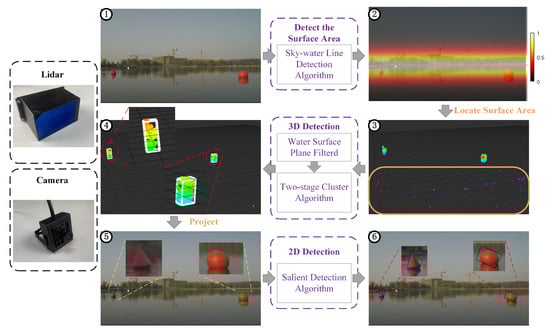
Figure 1. The flow of the detection framework. ① The image and point cloud are associated through an extrinsic matrix. ② The SSB detection method identifies the horizontal plane and determines the high-frequency region of the object. ③ Filter the water surface part in the point cloud. ④ A two-stage clustering algorithm is utilized to generate 3D boxes for water surface objects. ⑤ The detection results are projected into the image through the extrinsic matrix. ⑥ Through the 2D saliency object detection, the object position can be accurately obtained.

2.1. Calibration

To solve $R_{LC}$, the coordinates of the center point and the normal vector of the reference object in each sensor coordinate system must be obtained. Binocular cameras need to be pre-calibrated to establish internal parameters. In addition, the subsequent calculation also needs the length and width of the chessboard, as well as the number of corners and the size of each grid in the chessboard. We use the OpenCV built-in function [38] to determine the position of the checkerboard grid in the image and locate its edges and corners. The detected checkerboard edges and corners are combined with preset parameters as input to tackle the perspective-N-point problem (PnP). The output results include the calibrated center coordinate ${\mathbf{o}}_i^C$ and the normal vector ${\mathbf{n}}_i^C$, which accurately describe the position relationship of the checkerboard grid in the camera coordinate system.

For the LiDAR, we manually select a specific 3D region to ensure that the checkerboard is the only object within this range. To achieve this, we use the RANSAC algorithm to fit the point clouds in this region and generate a plane that accurately matches the checkerboard. The four vertices of this plane represent its extreme points. We then select four clusters that contain these extreme points and connect two points from each nearby cluster to obtain the edges of the fitted rectangular board. By calculating the variance of these fitted edges, we iterate until we find the edge and four vertices with minimal error. Additionally, for a given plane, we obtained both its center point coordinate $o_i^L$ by connecting diagonals and its normal vector ${\mathbf{n}}_i^L$.

To solve the overfitting problem, we rotate the chessboard through a specific angle to ensure that the normal vector is evenly distributed after each sampling. After repeating the process for many times, we obtain four groups of samples: ${\mathbf{N}}_L,{\mathbf{N}}_C,{\mathbf{O}}_L,{\mathbf{O}}_C$, each with a dimension of $d\ast 3$. Here, ${\mathbf{N}}_L,{\mathbf{N}}_C$ represent the matrices of normal vectors for the calibration board in the LiDAR and camera frames respectively, while ${\mathbf{O}}_L,{\mathbf{O}}_C$ correspond to the center points of the calibration board in the LiDAR and camera frames respectively. The extrinsic matrix can be described by Equation (1).

$$\begin{array}{c}\hfill {\mathbf{R}}_{LC}{\mathbf{N}}_L={\mathbf{N}}_C\\ \hfill {\mathbf{T}}_{LC}+{\mathbf{O}}_L={\mathbf{O}}_C\end{array}.$$

(1)

Here, the rotation and translation between multiple sensors are denoted by ${\mathbf{R}}_{LC}$ and ${\mathbf{T}}_{LC}$, respectively. While ${\mathbf{T}}_{LC}$ can be directly computed, the ${\mathbf{R}}_{LC}$ can be obtained using the following formula:

$${\mathbf{R}}_{LC}={\left({\left({\mathbf{N}}_L{{\mathbf{N}}_L}^T\right)}^{-1}{\mathbf{N}}_L{{\mathbf{N}}_C}^T\right)}^T.$$

(2)

In order to obtain more accurate extrinsic parameters, we incorporate the estimated values into the sample set and optimize until the error is minimized. Eventually we can fuse the point cloud and pixels through an extrinsic matrix, as shown in Figure 2

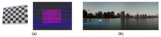
Figure 2. Through joint calibration, the extrinsic matrix of the sensor can be computed, this enables projection of the point cloud onto the corresponding image pixel. (a) Reference frames in camera and LiDAR. (b) The point cloud is projected onto the image through an extrinsic matrix.

2.2. Water Surface Removal

LiDAR generates point clouds by emitting lasers and receiving echoes reflected by objects. When the unmanned surface craft is in open water, the reflection intensity is low, and the LiDAR may not be able to form point clouds. On the contrary, at a relatively short distance, the point cloud formed by the water surface echo may lead to false detection, which is regarded as the interference that needs to be removed. Figure 3 compares the state of water surface point cloud before and after filtering.

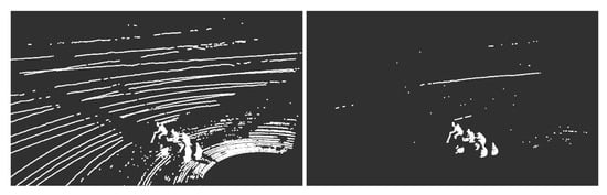
Figure 3. Water surface point cloud before and after filtering.

In order to estimate the horizontal plane of a water surface from a point cloud, we follow these steps:

• Identify the lowest points in the point cloud as they typically represent the water surface. Calculate their average height.
• Select candidate points within a specific range around this average height for plane fitting. Randomly sample several points from these candidates to construct and fit a plane model.
• Measure the distance between each point and the fitted plane using all candidate points as input for evaluation.
• Record interior points whose distance is below a certain threshold and count their number.
• If the current model has more interior points than the previous one, update its parameters and retain it as the best model so far.
• Repeat steps 2–5 until either reaching a set termination iteration limit or finding the model with maximum interior points.
• Once we have estimated the horizontal plane, identify any remaining points that are within $\epsilon$ distance from this plane and consider them part of the water surface; remove them from original point cloud.

2.3. Horizontal Plane Detection

Due to the limited density of distant point clouds, the camera can be used as an auxiliary tool of LiDAR to detect distant objects. In a single underwater image, the object is often distributed near the sky-sea boundary, which usually presents the maximum vertical gradient of pixel value. Therefore, we use the SSB detection algorithm to identify areas where there may be distant objects, and then the detection work based on point cloud analysis will mainly focus on these areas. The calculation formula of pixel gradient is as follows:

$$\begin{array}{c}{g}_x(x,y)=|I(x+1,y)-I(x-1,y)|\hfill \\ g_y(x,y)=|I(x,y+1)-I(x,y-1)|\hfill \end{array}.$$

(3)

Here, $g_x(x,y)$ denotes horizontal gradients, $g_y(x,y)$ represents vertical gradients and $I(x,y)$ refers to the grayscale value of a pixel point $(x,y)$. The points with larger gradients in the vertical direction are selected as candidates for fitting the SSB. The initial fitting point is established by selecting the pixel with the maximum local gradient among candidate points, followed by regional growth in the gradient direction within the neighborhood. Upon identifying a series of points on the SSB, the least squares method is utilized to obtain the final results, and we construct the error $err$:

$$err=\sum _{j=1}^m\left|y_j-\left(\widehat{a}{x}_j+\widehat{b}\right)\right|.$$

(4)

In this case, m represents the number of fitted points. The parameters a and b denote the final straight-line parameters, while $x_j$ and $y_j$ represent coordinate truth values. After completing SSB estimation, the next step is to define a distance within the range of ${\displaystyle \frac{height}{8}}$ along the vertical direction of the line as the potential region for object distribution. Here, $height$ refers to the height of the image. Then, the coordinate system is transformed into a point cloud coordinate system based on the external transformation matrix. In the subsequent detection process, we increase the clustering radius of the point cloud in the region to ensure that the sparse point cloud can be detected even at a longer distance.

2.4. Two-Stage Point Cloud Clustering Algorithm

After preprocessing, the point cloud data generated by LiDAR is used to identify obstacles on the water surface. In order to achieve real-time detection with low computational cost, the scheme based on clustering is more suitable. At present, Euclidean distance clustering method is widely used as a density based algorithm because of its robustness and fast response characteristics. Through calculating the distance between two points in two spaces, points can be determined whether they belong to the same object through threshold comparison.

However, in complex scenes, most methods are prone to producing false-positives, especially when multiple objects are densely distributed. Therefore, we propose a two-stage detection framework: The first stage uses Euclidean distance clustering algorithm to achieve fast object detection. In the second stage, the depth map adaptive threshold clustering algorithm is used to fine segment the small area.

First stage clustering module.The Euclidean clustering algorithm is utilized as the first stage detector for point cloud object detection. It takes inputs such as the clustering radius R, the minimum number of points $\eta$ in a cluster and the filtered point cloud set $P_{sur}$ after removing water surface points. However, in reality, the collected point cloud is not uniform and becomes sparser as it gets farther from the unmanned ship. Using the same parameters for distant objects could result in false detections. To address this issue, we modify the algorithm by making the clustering radius distance-adaptive, allowing for a larger threshold for distant objects. The first stage clustering method is described in Algorithm 1. Each point in $P_{sur}$ is assigned a number to facilitate later classification. An initial center point $p_i\in P_{sur}$ is selected, and a non-empty neighborhood with radius r is constructed around it. All points within this neighborhood are added to a cluster, and this process continues until no new points are found within radius r. These points are then grouped together and labeled under a specific category representing their cluster. If a cluster has too few points, which may result in false detection, we delete it and move on to the next loop. Finally, the 3D bounding box of the detected object is obtained based on the extreme value of the coordinates of the points inside the clusters.

Algorithm 1: Euclidean clustering.

Second stage clustering module. The Euclidean clustering method has a significant effect on the distribution of objects scattered on the water surface. However, when multiple objects are closely adjacent, this method is difficult to distinguish a single object from multiple objects. Although this limitation does not affect the obstacle detection of unmanned ship, it is still a defect. To solve this problem, we developed a two-stage point cloud detection scheme called depth map adaptive threshold clustering method. Compared with the previous stage method, this scheme significantly improves the object segmentation accuracy and the overall detection effect.

When the detected 3D bounding box may contain multiple objects, and the distance between adjacent objects is less than the clustering radius, different horizontal and vertical resolutions will lead to the difference in the distance between points in each direction. As shown in Figure 4, directly adopting the same clustering radius will directly increase the risk of misjudgment. This strategy combines point cloud distribution and attribute information to identify discontinuities between points. In addition, the method also considers the multi-azimuth resolution and accurately adjusts the clustering radius to accurately detect the point cloud of adjacent objects.

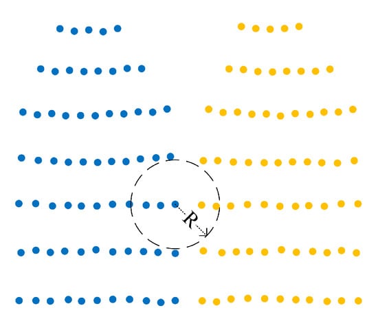
Figure 4. Point clouds have lower resolution in the vertical direction, applying same radius may cause a false detection.

When there is a discontinuity between points, the coordinate values should change abruptly. In Case 1 of Figure 5, as the clustering algorithm becomes more tolerant of offsets in the X-axis dimension and stricter with offsets in other axis dimensions, the distribution of points satisfying the clustering criterion shifts from spherical to elliptical. This dynamic adjustment improves the ability to identify discontinuities and reduces misclassification. The same principle applies when performing clustering in the vertical dimension, where more attention is given to axes without fixed offsets, as shown in Case 2 of Figure 5.

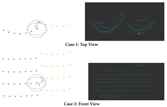
Figure 5. Two cases of cluster radius.

To address the issue of an unordered set of points in a point cloud, we convert it into a hash table format. This format resembles a 2D image with pixels arranged in predetermined patterns. Each element in the hash table contains coordinates, intensity and line count per point in the point cloud. This structured representation improves searchability and efficiency. For input point cloud data, we introduce a hash table with dimensions H (number of scan lines) and W (horizontal resolution of LiDAR). The index for each element $(row,col)$ in the hash table can be represented as follows:

$$index=row\times W+col.$$

(5)

After clustering the point cloud data in the first stage, the resulting clusters can be transformed into a hash table format. Each row in the hash table represents a group of points on the same horizontal plane under realistic conditions. The maximum number of points in a single row is denoted as $den$. The $line$ property within the point cloud attributes indicates the laser beam number to which each point belongs. The difference in line numbers between points within a cluster is defined as $\Delta L$. By considering the parameters $den$ and $\Delta L$, we can approximate the shape of the point cloud.

A point p$(x,y,z)$ in space can be represented in polar coordinates as $(r,\phi ,\theta )$, where r is the distance of the point and $\phi$ and $\theta$ are the vertical and horizontal angles from the point to the plane, respectively. In sensing system, the following transformation hold:

$$\begin{array}{c}x=r^{*}cos{\phi }^{*}sin\theta \hfill \\ y=r^{*}cos{\phi }^{*}cos\theta \hfill \\ z=r^{*}sin\phi \hfill \end{array}.$$

(6)

To adapt to the sparsity of point clouds at greater distances, we adjust the clustering radius accordingly. We achieve this by applying a density-based adaptive thresholding method, which was originally proposed for 2D detection [39,40], to 3D clustering approach. In Figure 6, $p_i$ represents the current centroid, while $p_{i+1}$ is randomly distributed in space as proximity points. The angle $\Delta \varphi$ between these two points and the origin corresponds to the angular of LiDAR resolution. By modifying the custom parameter $\lambda$, we can obtain a more precise area-adaptive clustering scale R. This relationship can be deduced from Figure 6:

$$\begin{array}{cc}\hfill R·sin(\lambda -\Delta \varphi )& =O{p}_i·sin(\Delta \varphi )\hfill \\ \hfill R& =O{p}_i·{\displaystyle \frac{sin(\Delta \varphi )}{sin(\lambda -\Delta \varphi )}}.\hfill \end{array}$$

(7)

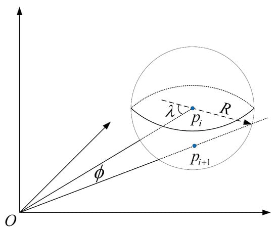
Figure 6. When the parameter $\lambda$ is constant, the dynamic clustering radius is only related to the angular resolution $\varphi$ of the LiDAR and the range of the current point.

When $\lambda ={91}^{\circ }$, it can be ensured that the neighborhood radius needs to grow approximately linearly with distance and that each clustered neighborhood contains a sufficient number of points.

In Algorithm 2, we describe the second stage of clustering. This stage involves building a hash table, which is achieved from line 1 to line 10. Once the hash table construction is complete, the search for neighbors takes place. Figure 4 illustrates that the point clouds have varying resolutions in the horizontal and vertical dimensions. To account for this, different parameters $\lambda$ are used in different directions, as indicated in line 16 and line 17.

Algorithm 2: The Second Stage Clustering.

Considering the distribution of point cloud data, we have designed an elliptical mask that closely matches the shape of current point cloud clusters. The purpose of this design is to minimize empty elements within the hash table and maximize neighboring elements relevant to each current point during neighborhood searches. Equation (8) represents the expression for this designed mask.

$$S_1{\displaystyle \frac{{\left(row-ro{w}_0\right)}^2}{de{n}^2}}+S_2{\displaystyle \frac{{\left(col-co{l}_0\right)}^2}{\Delta L^2}}\le 1.$$

(8)

where $(ro{w}_0,co{l}_0)$ is the current center point in hash table and $S_1$ and $S_2$ are the scaling parameters. $den$ and $\Delta L$ are obtained above to represent the horizontal and vertical shape of the point cloud. $S1$ and $S2$ constrain the pitch and azimuth differences between pairs of points, respectively, and are used to filter across objects or noisy points; since LiDAR has a much lower pitch resolution, $S1=8$ and $S2=0.6$ are taken to ensure that the masks cover similar numbers of valid neighboring points at different distances.

Since there are varying resolutions in the hash table for both horizontal and vertical dimensions, different clustering criteria need to be developed. Additionally, as points move away from the center point within a neighborhood, their confidence level should decrease. Equation (9) illustrates an elliptical heatmap centered on the current point, which has the same shape as the previously mentioned mask design. The intensity value at its center is 1, gradually decreasing towards its edges. Equation (9) provides each element’s heat value, as shown in Figure 7.

$$f(row,col)=e^{-\left(S_1{\displaystyle \frac{{\left(row-ro{w}_0\right)}^2}{de{n}^2}}+S_2{\displaystyle \frac{{\left(col-co{l}_0\right)}^2}{\Delta L^2}}\right)}.$$

(9)

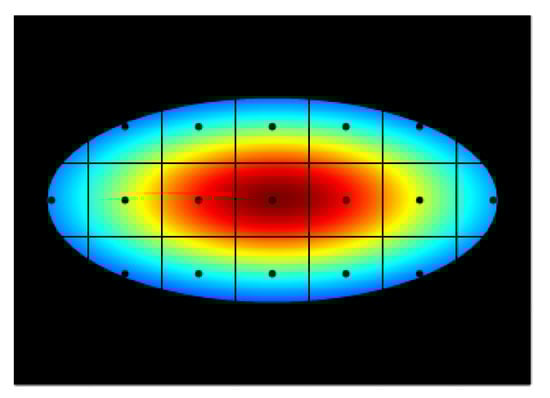
Figure 7. An elliptical heat map was created, emphasizing the areas closer to the center more.

Algorithm 2 outlines the second stage of clustering, which involves conducting neighborhood searches for each element in the hash table. To identify points within the same cluster, two criteria must be met: first, the distance between two points should be less than the clustering radius defined in Equation (10).

$$\begin{array}{c}\hfill \sqrt{{\left(\left|row-ro{w}_0\right|*R_{hor}\right)}^2+{\left(\left|col-co{l}_0\right|*R_{ver}\right)}^2}\\ \hfill \ge dis\ast hea{t}_{(row,col)}^{-1}\end{array}.$$

(10)

where $dis$ is the relative distance between two points, $heat$ is the value calculated from the heat map and $R_{hor}$ and $R_{ver}$ denote the cluster radius in the horizontal and vertical directions, respectively. An additional criterion for identifying whether points within a neighborhood belong to the same category is that consecutive angle changes should be below a given threshold, as shown in Equation (11).

$$\begin{array}{c}\hfill \left|arctan\left({\displaystyle \frac{\sqrt{\Delta x^2+\Delta y^2}}{\Delta z}}\right)\right|<t{h}_{ag1}\\ \hfill \bigcup \left|arctan\left({\displaystyle \frac{\Delta y}{\Delta x}}\right)\right|<t{h}_{ag2}\end{array}.$$

(11)

where both $t{h}_{ag1}$ and $t{h}_{ag2}$ are threshold parameters. Only when both of the above criteria are satisfied will the points be labeled as belonging to the same category. Moreover, $t{h}_{ag1}={12}^{\circ }$ and $t{h}_{ag2}=6^{\circ }$ for filtering across objects or noise points.

In the above clustering process, only points that strictly meet the criteria will be marked as part of the cluster. This means that only points that are adjacent to each other will be grouped and points that deviate slightly from the group may not be marked as belonging to the same object. Unmarked points do not belong to any category and need to be further distinguished. Therefore, we finally identify all unmarked points based on the distribution and characteristics of the marked points.

Considering the characteristics of the LiDAR point cloud, it can be inferred that the points on the water surface and the object are usually distributed on a plane or smooth surface. So we regard these points in the cluster as points on the same plane. To determine the plane, we use the extreme points in the point cloud cluster to find the center point O and then use the RANSAC plane fitting algorithm to fit and identify the best model of the plane. At the same time, the normal vector ${\mathbf{V}}_{nor}$ of the fitting plane is obtained.

For both labeled and unlabeled points within this cluster, we connect them with either their centroid or with centroid of their respective planes to form vectors $V_P$. These vectors should ideally have a dot product value of 0 when compared with their corresponding planes’ normal vector ${\mathbf{V}}_{nor}$. The calculation for this dot product is shown in Equation (12), illustrated in Figure 8.

$$\begin{array}{c}\hfill angle={\displaystyle \frac{\left|{\mathbf{V}}_1·{\mathbf{V}}_2\right|}{\left|{\mathbf{V}}_1\right|·\left|{\mathbf{V}}_2\right|}}.\end{array}$$

(12)

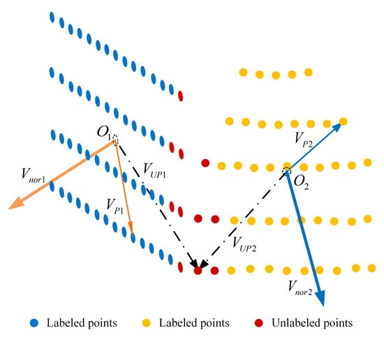
Figure 8. ${\mathbf{V}}_{UP1}$, ${\mathbf{V}}_{UP2}$ are normal vectors, and unlabeled points are classified by their product.

If the $angle$ is greater than a threshold, the point is considered to not belong to the plane; otherwise, the point is identified as belonging to the current cluster. If there are multiple clusters that meet this condition, the unlabeled point will be compared with each plane, as shown in Figure 8, and assigned to the cluster with a smaller angle. This process results in obtaining the refined 3D bounding box $B{B}_i$.

2.5. Saliency Detection

In order to achieve accurate segmentation of water surface objects, we combine the coordinates obtained by LiDAR with the fine features captured by camera. The proposed method uses the point cloud detection results as the input to detect the prominent objects on the water surface. This scheme can effectively correct the detection results and achieve accurate segmentation, so as to realize water surface object detection by fusing LiDAR and camera data.

In order to reduce the interference of reflection, overexposure and other factors on saliency detection in the whole image, we project the 3D point cloud detection results to the image to define the candidate region. In this way, the detection range is reduced and the external interference is successfully avoided. However, due to the extrinsic matrix error, the projection area may not fully contain the real object. To solve this problem, we expand the projection area in proportion before implementing the saliency object detection algorithm.

From a visual point of view, areas with unique characteristics tend to be more prominent in the image. The saliency detection algorithm quantifies the contrast between the foreground and the background by using the differentiated saliency value. After obtaining the region of interest with significant color contrast between the object and the background, we use the global contrast saliency detection algorithm. In the image taken on the water surface, the background can be regarded as low-frequency information but may contain high-frequency noise components. The object belongs to a high-frequency signal relative to the background. Our goal is to filter high-frequency noise and low-frequency background signals so as to identify objects with the largest significant area. Therefore, the accurate selection of bandpass filter parameters is very important [41,42].

We use the combination of multiple Gaussian differences as bandpass filters. A single Gaussian filter can be expressed as Equation (13).

$$\begin{array}{cc}\hfill DoG(x,y)& ={\displaystyle \frac{1}{2\pi }}\left[{\displaystyle \frac{1}{{\sigma }_1^2}}{e}^{-{\displaystyle \frac{\left(x^2+y^2\right)}{2{\sigma }_1^2}}}-{\displaystyle \frac{1}{{\sigma }_2^2}}{e}^{-{\displaystyle \frac{\left(x^2+y^2\right)}{2{\sigma }_2^2}}}\right]\hfill \\ \hfill & =G\left(x,y,{\sigma }_1\right)-G\left(x,y,{\sigma }_2\right)\hfill \end{array}.$$

(13)

where ${\sigma }_1$, ${\sigma }_2$ are the standard deviation, the filter whose bandpass width is determined by ${\sigma }_1:{\sigma }_2$, suppose ${\sigma }_1=\rho \sigma , {\sigma }_2=\sigma$. Each time the Gaussian function is executed, it is equivalent to a bandpass filter to find out the potential location of the object in the image. The full bandpass filter can be expressed as follows:

$$\sum _{n=0}^{N-1}G\left(x,y,{\rho }^{n+1}\sigma \right)-G\left(x,y,{\rho }^n\sigma \right).$$

(14)

Gaussian filtering is performed N times on different scales and summed to filter as much noise and background as possible so that the location of the object is more prominent. The original and Gaussian filtered images are then transformed into $Lab$ space, and the final saliency score of each pixel on the image can be expressed as Equation (15).

$$S(x,y)=\Vert I_{ave}-I_{Gau}(x,y)\Vert .$$

(15)

$I_{ave}$ is the arithmetic mean of pixels in $Lab$ space and $I_{gau}$ means is the result of Gaussian filtering in $Lab$ space. The largest connected region with a pixel score above the threshold should be the location where the actual object.

3. Results

This chapter mainly introduces the preparation requirements for conducting experiments, including the USV platform, the hardware devices for collecting data, and the evaluation criteria for validation experiments. Subsequently, we collected real-world water surface data and simulated data to evaluate our algorithm.

3.1. Experiment Platform Description

Figure 9a shows the catamaran we selected for the object detection experiment. We collect data in the real lake environment. The object objects include buoys, small ships and other common surface objects. At the hardware level, the perception system of the unmanned ship includes stereo camera, laser radar and Intel NUC computing platform, and all devices are driven by battery powered DC power. All programs run in Ubuntu system, and the collected data is processed in ROS message or rosbags format. The camera is installed at the front of the hull about 1.2 m away from the water surface, with a resolution of 1080 × 720 and is connected to the host (i7-8559U) in the control box of the unmanned ship through USB cable.

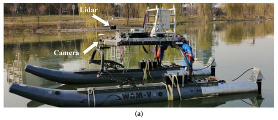
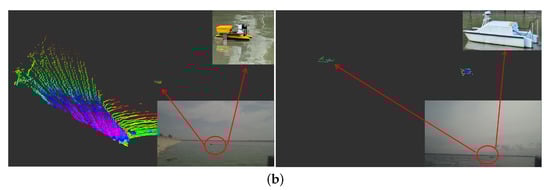
Figure 9. Sensing system and experimental data. (a) USV equipped with LiDAR and a camera. (b) Samples of the collected data.

The experiment uses Leishen 64 line high-resolution LiDAR (Leishen Intelligent System Co., Ltd., Shenzhen, Guangdong, China), which is installed on the support rod in front of the deck. The maximum detection distance is 130 m, the horizontal field angle is 120 degrees and the vertical field angle is 21 degrees. At 5 Hz operating frequency, the average vertical resolution is 0.33 degrees and the horizontal resolution is 0.09 degrees. The LiDAR is connected to the main control computer through RJ-45 interface. The data acquisition and algorithm processing are implemented by c++language in Ubuntu system environment, and the subsequent processing is completed by OpenCV3 and point cloud Library (PCL). The computing platform reads the original data from the port through the driver and publishes it in the form of topics in the robot operating system (ROS) environment. The algorithm obtains data by subscribing to these topics, and after processing, the results are published as ROS topics. In the subsequent comparison experiments, the training and computing platforms for all learning-based methods were performed on a mainframe computer with an Intel XEON 4110 CPU and two 3080Ti GPUs.

In view of the uncertainty of the state and position of water surface objects, it is difficult to detect small objects, and the data acquisition covers the observation conditions of different distances and angles.

3.2. Data Description

Water surface object detection algorithm may be interfered by overexposure, underexposure, reflection and other factors. In order to ensure the robustness of the algorithm, we carried out large-scale data acquisition in the real water environment and a variety of weather scenes, aiming to cover all the scenes that may be encountered in water surface object detection, and verify the effectiveness of the multi-sensor fusion detection method. Using this platform, we collected 5020 sets of synchronized point clouds and images in reservoirs, lakes and inland waterways. The data collected included common objects on the water, including objects such as buoys, small- to medium-sized unmanned vessels (less than 10 m) and large vessels (over 30 m), covering the types of objects common to USV autonomous navigation. The target distribution distance is mainly concentrated in the interval of 30–60 m, but there are still 28.6% of the data in the interval of 60–100 m, in order to better quantify the performance of the algorithm under different distances. In addition, the number of targets in a single frame varies from 1 to 15, and 21.5% of the data are adjacent to multiple targets or targets adjacent to the shore to verify the robustness in complex situations. Figure 9b shows examples of the collected data, including synchronized waterborne LiDAR and point cloud data.

3.3. Evaluation Metric

Intersection of union (IoU) is used as a measure to describe the degrees of overlap between two boxes, the true positive cases are the boxes whose IoU exceeds the threshold. In this experiment, the evaluation metrics are the same as traditional object detection, using precision and recall as performance metrics. $TP,FP,FN,TN$ denote, respectively, correctly detected objects, false alarms, missed alarms and correctly ignored backgrounds.

$$Precision={\displaystyle \frac{TP}{TP+FP}}, recall={\displaystyle \frac{TP}{TP+FN}}.$$

(16)

In Equation (16), precision is defined as the ratio of detected positive cases to all detected samples, while recall represents the probability of being predicted to be positive in an actual positive sample.

Since the detection framework is oriented to the water surface environment, missed or false detections have a negative impact on USV navigation. To more fully measure the performance of the algorithm, we include false positive rate and true positive rate in the evaluation metrics.

$$FPR={\displaystyle \frac{FP}{FP+TN}}, TPR={\displaystyle \frac{TP}{FN+TP}}.$$

(17)

As defined in Equation (17), the false positive rate (FPR), or false alarm rate, is the proportion of positive samples with wrong predictions of all positive. While true positive rate (TPR) indicates the percentage of correctly detected objects. In addition, we also used mean average precision ($mAP$) to evaluate the performance of the algorithm.

RMSE (Root Mean Square Error) and mIoU reflect the deviation between the estimated center and the ground truth, RMSE is defined as follows:

$$RMSE=\sqrt{{\displaystyle \frac{1}{n}}{\sum }_{i=1}^n\left[{\left(x_i-{\widehat{x}}_i\right)}^2+{\left(y_i-{\widehat{y}}_i\right)}^2+{\left(z_i-{\widehat{z}}_i\right)}^2\right]}$$

(18)

3.4. Result Analysis

3.4.1. Qualitative Analysis

We evaluate the performance of the algorithm on the collected data sets. In this work, the image-based sky–sea boundary detection technology is applied to provide the object area for the LiDAR and then uses the clustering detection technology based on point cloud to obtain the three-dimensional boundary of the object, effectively reducing the detection range. The saliency detection algorithm is applied in the object region to determine the precise position of the object.

Figure 10 presents several qualitative analyses of the results. Figure 10a showcases the results achieved by using Euclidean clustering followed by saliency detection, while Figure 10b illustrates how changing to the proposed clustering algorithm improves these outcomes. A comparison between these results highlights two major advantages:

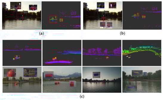
Figure 10. Qualitative analysis of the detection algorithm on the collected dataset. (a) False detection due to multiple objects in close proximity. (b) Multiple objects correctly labeled. (c) More visualization results.

Firstly, even underexposed objects on water surfaces can still be detected due to multi-sensor fusion capabilities. Secondly, our method accurately distinguishes boundaries between objects that are situated at extremely close distances, as demonstrated in Figure 10c.

3.4.2. Quantitative Analysis

Table 1 shows the excellent performance of this algorithm in water surface object detection. The overall detection accuracy of all objects in the data set is 0.938, especially in the detection of common small ships. The method has efficient detection capability for typical surface objects and effectively detects common objects on the water surface through multi-sensor fusion technology to realize accurate segmentation of objects in the image. In addition, we combine the LiDAR detection results to realize the identification of sky and sea lines and the delineation of camera candidate areas so that the advantages of each sensor complement each other and form a better solution suitable for a variety of scenes.

Table 1. Accuracy of detection method in different scenes.

Reflection	Underexposure	Overexposure	Adjacent Objects
0.921	0.937	0.934	0.919

Table 2 shows the detection accuracy performance of the algorithm under different water surface conditions. The two-dimensional detection algorithm can effectively avoid the impact of water surface reflection or overexposure by generating pre-detection areas for optical sensors through LiDAR. As shown in Figure 10a, false detection caused by adjacent objects is a common problem. For this reason, we developed an effective clustering method, and the results show that the scheme significantly improves the practicability while maintaining the accuracy.

Table 2. Accuracy of detection method for different objects.

Buoy	Surface Vessels	Floating Objects	Average
0.941	0.942	0.925	0.938

3.4.3. Comparison of Clustering Algorithms

Unlike other detection tasks, our focus is on the distribution of surface obstacles because unmanned surface craft need to avoid obstacles. Frequent false alarms will lead to the unmanned craft unable to navigate along the normal track, and missing alarms will directly threaten the safety of the ship. Therefore, the false positive rate and accuracy rate are two key indicators to evaluate the performance of the algorithm.

In theory, the main reason for false positives is that the algorithm fails to fully filter plane features, resulting in a single point may be misjudged as the object object. Under reporting results from the fact that the point cloud data is not enough to form an independent object object, or only a part of the real object is detected, which leads to the low IoU of the annotation and reduces the detection accuracy.

In order to compare the performance of different clustering algorithms, we changed the clustering method and tested the water surface data set while keeping the two-dimensional saliency detection algorithm unchanged. Figure 11 shows the experimental results of various algorithms. When the intersection union ratio threshold is set to 0.8, the algorithm outperforms other clustering algorithms in terms of lower false positive rate and better detection accuracy. This confirms that the dynamic adjustment of radius and the weight of ellipse thermal diagram can improve performance. Even in the case of the worst performance, the accuracy rate of 0.801 and the false positive rate of 0.194 are still achieved. This highlights the advantages of multi-sensor fusion method over simple two-dimensional detection method in ground object detection.

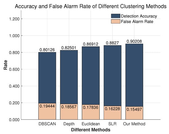
Figure 11. Comparison of false alarm rate with different clustering strategies.

Then we compared the accuracy rate, recall rate, false positive rate and true positive rate, and drew the precision-recall (PR) curve and receiver operating characteristic (ROC) curve, as shown in Figure 12a,b. The larger the area under the curve, the better the performance. Our clustering algorithm maintains significant advantages in all evaluation indicators. This two-stage clustering algorithm can obtain more accurate 3D boundary boxes of objects and reduce the false detection rate. When encountering adjacent objects, the algorithm can dynamically adjust the clustering range according to the size and density of objects, so as to capture the object boundary more accurately. By using the characteristics of point cloud, the point cloud data can be classified more accurately according to the characteristics of objects, and the accurate separation of adjacent objects can be realized. Experiments show that this method significantly improves the accuracy of object detection, especially in the adjacent object discrimination. This technology has broad application prospects in water surface object detection tasks.

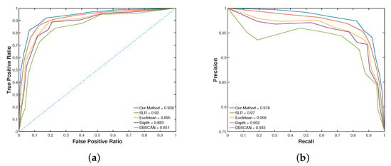
Figure 12. Performance comparison of the proposed method and other methods. (a) ROC curve comparison. (b) PR curve comparison.

In this study, we collected data from different scenarios to verify the performance of the algorithm in this work. Without changing the two-dimensional detection algorithm, we compared the effectiveness of various clustering methods in complex water scenes. Figure 13 shows that all object detection algorithms based on multi-sensor fusion perform well. However, the proposed clustering method achieves higher accuracy and optimized detection performance, especially when dealing with adjacent objects. The advantages of our method are not only limited to water surface image processing but can also be applied to other tasks such as geometric structure object detection based on point cloud. Experimental results show that our clustering algorithm can effectively improve the accuracy and robustness of multi-sensor fusion detection algorithm.

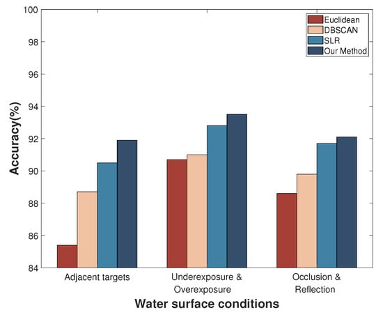
Figure 13. Comparison of accuracy with different clustering strategies for challenging scenarios on water surfaces.

The detection technology based on point cloud can eliminate the light interference and provide distance information for the channel planning of USV. In addition, the two-dimensional image can achieve more accurate object positioning and record object features for subsequent processing. When the traditional point cloud clustering algorithm deals with the adjacent objects on the water surface, it often regards the adjacent objects as a single entity. The two-stage detection method proposed in this paper can effectively separate these adjacent point cloud clusters. In all experiments, this method shows high accuracy and wide applicability, which further verifies the theoretical deduction. The fusion of 3D point cloud and 2D image information is expected to improve the navigation performance of unmanned surface vehicles and ensure safer and more efficient path planning in complex water environment.

As shown in Table 3, the method proposed in this paper achieves the best performance in various obstacle detection tasks, especially in complex scenes. Traditional methods, relying solely on density or distance metrics, perform poorly when dealing with objects with complex geometric shapes. However, adaptive distance metrics and clustering methods that combine object shapes effectively distinguish between real floating objects and surface wave interference.

Table 3. Comparison with other algorithms.

Method	Buoy	Surface Vessels	Floating Objects	Average
DBSCAN	0.928	0.930	0.825	0.851
Depth	0.934	0.932	0.833	0.883
Euclidean	0.938	0.937	0.840	0.895
SLR	0.940	0.935	0.894	0.920
Ours	0.941	0.942	0.925	0.938

By randomly selecting a fixed number of data samples and computing the 95% confidence interval to assess result reliability, 10 independent replicate tests are conducted. The average serves as the final performance metric, yielding the results shown in the Figure 14. As the sample number increases, the average accuracy of all methods rises until it stabilizes, while the confidence interval width gradually narrows, indicating that algorithmic fluctuations tend toward stability. In comparison, our method demonstrated optimal stability and reliability across multiple repeated tests, thus confirming its effectiveness and robustness.

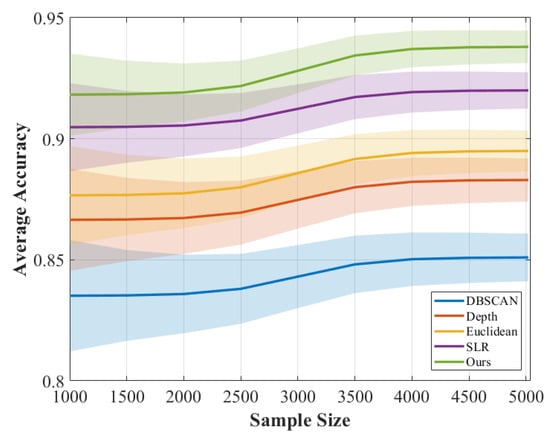
Figure 14. Analysis of sample size on performance and 95% confidence intervals.

3.4.4. Comparison of Learning-Based Algorithms

The performance of the algorithm is analyzed over different distance intervals using the already trained model weights, fine-tuned on the collected dataset. As shown in Table 4, the method in this paper achieves the highest mAP in all distance intervals, especially in the middle and long distances with significant advantages. Although its RMSE is slightly inferior to some learning-based methods, the mIoU is not much different from mainstream methods, and the real-world environment, where the priority is to detect correctly without pursuing finesse on the edges, indicating that the localization accuracy and segmentation quality are balanced. However, as the distance increases, the performance decays significantly slower than other methods. As shown in Figure 15, the detection results in the first column show that the method in this paper has more fine segmentation for neighboring objects, and the learning-based method is difficult to cover all objects, especially the more sparse water surface point cloud, because of the difficulty in obtaining data. In the second column, although the bounding box fit of the learning-based method is higher, the proposed method also detects the objects in a similarly complete manner, achieving a better balance between detection recall and geometric accuracy.

Table 4. Performance comparison across different distance ranges (mAP@0.5:0.8).

Dist.	3D-SSD			Voxel R-CNN			PVRCNN++			Proposed
	mAP ↑	mIoU ↑	RMSE ↓	mAP ↑	mIoU ↑	RMSE ↓	mAP ↑	mIoU ↑	RMSE ↓	mAP ↑	mIoU ↑	RMSE ↓
0–20 m	73.3	0.88	0.18	78.7	0.91	0.21	81.2	0.89	0.12	89.7	0.88	0.20
20–40 m	58.5	0.83	0.31	62.1	0.86	0.29	64.8	0.87	0.27	86.3	0.80	0.37
40–60 m	50.2	0.82	0.39	53.5	0.83	0.37	56.2	0.85	0.30	79.5	0.78	0.46
60–80 m	37.8	0.73	0.52	41.9	0.77	0.50	48.1	0.78	0.47	72.8	0.72	0.68
>80 m	30.1	0.69	0.77	33.5	0.73	0.69	5.7	0.74	0.61	68.2	0.69	0.85

↑: higher is better, ↓: lower is better. Bold: best in each distance range.

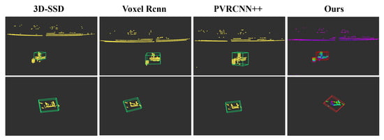
Figure 15. Visualization of comparison with other DL-based methods.

3.4.5. Robustness and Real-Time Analysis

To evaluate the real-time performance, we tested it on the same hardware as the data acquisition device (Intel NUC i7). We randomly selected 500 frames of real water surface point cloud data to simulate the water surface scene and, finally, obtained an average running time of the algorithm of 82.7 ms. The results are shown in the Table 5. The clustering stage dominates the overall computation, accounting for approximately 75–83% of the total processing time. Clustering takes a long time because it contains more voxels at a long distance, but it does not exceed the LiDAR operating frequency (5 to 10 Hz) in any case. In general, the detection framework we designed still has real-time performance on a single CPU host, which is very important for the actual work requirements of small- and medium-sized unmanned ships.

Table 5. Runtime breakdown across distance ranges (ms).

Distance	Clustering	SSB Detection	Saliency Detection	Average Processing Time
0–20 m	48.1	2.1	9.1	59.3
20–40 m	55.3	2.3	9.8	67.4
40–60 m	58.2	2.4	10.2	70.8
60–80 m	65.6	2.6	11.3	79.5
>80 m	80.2	2.8	13.7	96.7
Per frame	67.5	2.4	12.8	82.7

3.5. Ablation Study

3.5.1. SSB Module

In the complex water surface scene, the image is often interfered by external factors, and the two-dimensional detection algorithm is prone to produce high false-positive rate. The point cloud based detection method significantly improves the robustness by identifying RoIs first, so that USVs can perform tasks in diverse scenarios.

In order to verify the usefulness of the SSB detection method in the image for the whole multi-sensor detection framework, we replace several different clustering algorithms and compare the detection accuracy before and after the addition of the sky–sea boundary detection algorithm, and the results are shown in Figure 16. From the results, it can be concluded that each type of clustering algorithm has some degree of improvement in accuracy after adding the SSB detection algorithm. Although some of the gains are relatively small in magnitude, it can be shown that this sky–sea boundary detection algorithm provides a priori information for the subsequent point cloud based detection and plays a positive role.

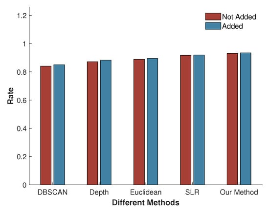
Figure 16. The accuracy of the clustering algorithm is improved by the SSB detection algorithm, reflecting the camera’s contribution to the LiDAR detection.

Experiments have demonstrated that the SSB module allows the detection scope to be focused on critical areas above and below the water surface by filtering the areas that are not related to the object in order to improve the anti-jamming capability.

3.5.2. Second Clustering Module

As shown in Table 6, the introduction of the two-stage clustering module brings accuracy gains across the range of distances, and the gains are particularly significant at close distances. In the 0–40 m interval, the module improves the detection accuracy by 4.3%, while in the 40–80 m and >80 m intervals, the improvement drops to 1.3% and 0.3%, respectively. This trend can be attributed to the physical properties of point cloud density and geometric features decaying with distance: in the close range region, the dense point cloud returned by LiDAR with rich structural details provides sufficient local information for two-stage clustering, thus suppressing over-segmentation or mis-merging, whereas in the mid-range and far-range, the point cloud is significantly sparse, and the number of sampling points on the object surface decreases, resulting in limited discriminative features available for advanced clustering strategies, and thus the two-stage stage optimization has progressively lower marginal benefits. Nevertheless, the module maintains consistent performance gains over the entire distance range, validating its adaptability to different perceptual scenarios.

Table 6. Ablation study on the two-stage clustering module (AP@0.5).

Conditions	0–40 m	40–80 m	>80 m	Overall
With two-stage clustering	0.921	0.885	0.841	0.892
Without two-stage clustering	0.883	0.872	0.838	0.868

Bold: best in each distance range.

The comparison of the running times with the learning-based methods is shown in Table 7, where our framework is run on an Intel i7-8559U CPU, while the other learning-based methods are run on an Nvidia 3080Ti. Although some methods can run in real time, the small computational cost makes lightweight methods easier to deploy and more advantageous in unseen scenarios.

Table 7. Runtime comparison of detection methods.

Metric	3D-SSD	Voxel R-CNN	PVRCNN++	Ours
Runtime (ms)	60.3	69.4	121.9	82.7

3.5.3. Hyperparameter Sensitivity

To evaluate the influence of hyperparameters on model performance and robustness, all parameters are adjusted in a fixed ±25% range around their baseline values. When analyzing the parameter sensitivity, only one parameter is changed at a time and the rest is kept constant, and the performance is measured by accuracy. The value of $\lambda$ varies within a range of 4%, the model’s performance is stable, with 3.2% reduction in accuracy, but little change in runtime. Beyond this interval, the performance drops significantly, especially when $\lambda$ is less than 80 or more than 102 (baseline is 91), the maximum accuracy drop is more than 11.4%. The reason is that its value needs to be strongly matched with the resolution of the sensor, and arbitrary adjustment will lose the connection with the sensor characteristics, resulting in the failure of the adaptive clustering radius.

The accuracy drop is small when the adjustment range of $S_1$ and $S_2$ is within 10% because its central role is to adjust the range of the ellipse heatmap, and slight changes will not directly affect the results. However, it is worth noting that if the increase exceeds 15%, the neighborhood range will be relatively large, the accuracy will be decreased by 6.2% and the operation time will also be increased by 4.3%.

$t{h}_{ag1}$ and $t{h}_{ag1}$ are the least sensitive among all parameters, which affect the ability to distinguish between adjacent targets. Because the smoothness of different point clouds varies greatly, the change of parameters within a reasonable range will not have a great impact on the performance.

4. Discussion

4.1. Model Performance and Method Adaptability

This study evaluated the performance of various surface obstacle detection strategies in complex water scenes. The results show that the proposed multi-sensor fusion framework shows significant advantages in the overall detection accuracy (0.938) and false alarm control. We focus on the real-time detection of water surface obstacles in complex waters and design the architecture based on the characteristics of the real scene rather than simply pursuing the improvement of accuracy. Specifically, we uses the two-stage architecture of laser radar guidance and image fine positioning, which effectively avoids the failure risk of pure vision method under the conditions of strong reflection, overexposure or underexposure. The 2D geometric information of the image is used to identify the sky sea line, and the 3D point cloud generates a reliable candidate detection region, which greatly reduces the image processing range and reduces the computational burden. On this basis, the designed dynamic radius clustering algorithm can adaptively adjust the clustering range according to the local point cloud density and object scale and significantly improve the resolution of adjacent obstacles. In contrast, the traditional fixed radius method is prone to merge misjudgment when dealing with dense small objects, while the end-to-end deep learning model often fails to detect in the sparse point cloud region due to the training data deviation. It is worth noting that the detection performance degradation of this method in the medium and long distance is significantly slower than that of the comparison model, which is very important for the forward-looking obstacle avoidance of USV. Although the RMSE of its boundary fitting is slightly higher than that of some learning methods, considering that the actual navigation pays more attention to whether there are obstacles rather than whether the edges fit at the pixel level, this balance between recall rate and geometric rationality is more in line with the engineering requirements. We acknowledge that although the data set used in this study covers a variety of water scenarios, the sample size is still limited and does not include test cases under extreme weather conditions. The stability of the framework is verified. Nevertheless, the current results should be regarded as the preliminary verification under the specific water environment, and its generalization ability should be further tested in the future under the wider geographical area and meteorological conditions.

4.2. Environmental Interference and Multimodal Complementary Mechanism

The core challenge of water surface obstacle detection is the strong spatio-temporal variability of environmental interference. Water reflection, sudden change of light, wave disturbance and other factors can easily lead to false positives in the pure vision system. The detection method relying only on 2D images is easy to misjudge on water, while the pure point cloud method is sparse and lack of texture on water. The proposed approach effectively solves the above problems through the complementary advantages of multi-sensor: LiDAR is not affected by light and can stably provide the three-dimensional spatial distribution of obstacles. The visible image has a high resolution, which can be used for precise positioning and object attribute recognition. In addition, the difference between the foreground and background of 3D point cloud projection, combined with the SSB detection module, fundamentally eliminates the interference sources below the water surface or in the sky area and only focuses on the area near the water surface. This design makes the subsequent saliency detection only run in the physically reasonable region, which greatly improves the robustness of the system. In the actual waters, obstacles often show the characteristics of spatial aggregation, similar scale and dynamic dense distribution, especially at the intersection of ports, fishing areas and waterways. In such scenarios, whether the adjacent objects can be accurately separated directly determines the rationality of the USV obstacle avoidance strategy. If the two parallel boats are misjudged as a single large obstacle, the USV may take excessive evasion, or even mistakenly enter the dangerous waters. The dynamic clustering algorithm proposed in this study is designed for this demand. By introducing the adaptive mechanism of the weight and local density of the elliptical thermal map, the algorithm can achieve more precise segmentation at the boundary of the point cloud cluster. We recognize that there are still challenges for the segmentation of non rigid or deformable objects in the current system. Similarly, clustering that only depends on geometric shape may also produce misjudgment on complex objects. Future work will explore the integration of object semantic information to enhance the recognition ability of heterogeneous obstacles and reduce the amount of computation through quantitative operation so as to facilitate the lightweight USV carrying.

4.3. Engineering Consideration and Management Enlightenment for Practical Application

Many unmanned tasks must be performed by small- and medium-sized USVs, but such ships are doomed to be difficult to carry high-capacity batteries and computing platforms. In this context, the traditional model with high map or low RMSE as the sole goal, although it performs well in the general data set, is difficult to be directly migrated to the actual water navigation task. The strategy of sensor complementarity and algorithm adaptation perfectly meets the challenges of water scene and the practical application requirements of USV. In addition to detection performance, real-time, hardware dependency and deployability are the key to determine whether the technology can be implemented. This framework achieves an average processing delay of 12 Hz on the single CPU platform, which meets the output frequency requirements of mainstream LiDAR without GPU acceleration. This feature makes it particularly suitable for small- and medium-sized, low-cost USV platforms, significantly reducing the entry threshold of intelligent navigation system. After experimental verification, the method proposed in this paper has the ability of practical application. According to practical experience, we believe that the multi-sensor fusion system should be preferentially deployed in high-risk areas such as inshore and port to deal with dense obstacles and strong light interference. In open waters, the processing frequency can be appropriately reduced to extend the endurance time. In addition, through the fine detection capability of this detection framework, a water obstacle database can be established to continuously collect point clouds and image features of different object types for online optimization of clustering parameters and saliency model. The ultimate goal is to build an interpretable, evolutionary and reliable water surface sensing system.

5. Conclusions

This paper proposes a fast water surface object detection method based on the fusion of point cloud and image data, which can complete the detection task in a wider range of water conditions and overcome the limitations of single sensor system in terms of high speed and high precision. Multi-sensor fusion enhances the anti-interference ability of the detection algorithm and optimizes the detection object boundary. The two-stage clustering algorithm based on point cloud data is designed to distinguish adjacent objects by mining the point differences between different objects and integrating local features, which is significantly better than the traditional method while meeting the real-time requirements. The data set is derived from the verification theory of real lake environment. The experimental results show that compared with the conventional clustering algorithm or surface object detection method, this method has more advantages in detection accuracy and anti-interference ability, especially in the detection of adjacent objects.

References

- Bedja-Johnson, Z.; Wu, P.; Grande, D.; Anderlini, E. Smart anomaly detection for slocum underwater gliders with a variational autoencoder with long short-term memory networks. Appl. Ocean Res. 2022, 120, 103030. [Google Scholar] [CrossRef]
- Liu, Q.; Ye, Z.; Zhu, C.; Ouyang, D.; Gu, D.; Wang, H. Intelligent target detection in synthetic aperture radar images based on multi-level fusion. Remote Sens. 2025, 17, 112. [Google Scholar]
- Huntsberger, T.; Aghazarian, H.; Howard, A.; Trotz, D.C. Stereo vision–based navigation for autonomous surface vessels. J. Field Robot. 2011, 28, 3–18. [Google Scholar]
- Chen, M.; Tang, Y.; Zou, X.; Huang, K.; Li, L.; He, Y. High-accuracy multi-camera reconstruction enhanced by adaptive point cloud correction algorithm. Opt. Lasers Eng. 2019, 122, 170–183. [Google Scholar] [CrossRef]
- Fefilatyev, S.; Goldgof, D.; Shreve, M.; Lembke, C. Detection and tracking of ships in open sea with rapidly moving buoy-mounted camera system. Ocean Eng. 2012, 54, 1–12. [Google Scholar] [CrossRef]
- Dong, R.; Fang, X.; Meng, X.; Yang, C.; Li, T. Enhancing underwater LiDAR accuracy through a multi-scattering model for pulsed laser echoes. Remote Sens. 2025, 17, 2251. [Google Scholar] [CrossRef]
- Bovcon, B.; Perš, J.; Kristan, M. Improving vision-based obstacle detection on usv using inertial sensor. In Proceedings of the 10th International Symposium on Image and Signal Processing and Analysis, Ljubljana, Slovenia, 18–20 September 2017; IEEE: Piscataway, NJ, USA, 2017; pp. 1–6. [Google Scholar]
- Bovcon, B.; Muhovič, J.; Vranac, D.; Mozetič, D.; Perš, J.; Kristan, M. MODS—A USV-oriented object detection and obstacle segmentation benchmark. IEEE Trans. Intell. Transp. Syst. 2021, 22, 7527–7539. [Google Scholar]
- Zhang, L.; Zhang, Y.; Zhang, Z.; Shen, J.; Wang, H. Real-time water surface object detection based on improved faster r-cnn. Sensors 2019, 19, 3523. [Google Scholar] [CrossRef] [PubMed]
- Zhang, X.; Wang, D. Visual saliency detection for water surface contaminants. In Proceedings of the 2020 3rd International Conference on Control and Robots (ICCR), Tokyo, Japan, 26–29 December 2020; IEEE: Piscataway, NJ, USA, 2020; pp. 43–47. [Google Scholar]
- Li, R.; Wu, J.; Cao, L. Ship target detection of unmanned surface vehicle base on efficientdet. Syst. Sci. Control Eng. 2022, 10, 264–271. [Google Scholar]
- Sun, X.; Liu, T.; Yu, X.; Pang, B. Unmanned surface vessel visual object detection under all-weather conditions with optimized feature fusion network in yolov4. J. Intell. Robot. Syst. 2021, 103, 55. [Google Scholar] [CrossRef]
- Li, Y.; Guo, J.; Guo, X.; Zhao, J.; Yang, Y.; Hu, Z.; Jin, W.; Tian, Y. Toward in situ zooplankton detection with a densely connected yolov3 model. Appl. Ocean Res. 2021, 114, 102783. [Google Scholar] [CrossRef]
- Liu, L.; Li, P. Plant intelligence-based pillo underwater target detection algorithm. Eng. Appl. Artif. Intell. 2023, 126, 106818. [Google Scholar] [CrossRef]
- Chen, X.; Wu, H.; Han, B.; Liu, W.; Montewka, J.; Liu, R.W. Orientation-aware ship detection via a rotation feature decoupling supported deep learning approach. Eng. Appl. Artif. Intell. 2023, 125, 106686. [Google Scholar] [CrossRef]
- Yang, L.; Wu, J.; Li, H.; Liu, C.; Wei, S. Real-time runway detection using dual-modal fusion of visible and infrared data. Remote Sens. 2025, 17, 669. [Google Scholar] [CrossRef]
- Shao, G.; Fei, S.; Shao, G. A robust stepwise clustering approach to detect individual trees in temperate hardwood plantations using airborne LiDAR data. Remote Sens. 2023, 15, 1241. [Google Scholar] [CrossRef]
- Jin, X.; Yang, H.; He, X.; Liu, G.; Yan, Z.; Wang, Q. Robust LiDAR-based vehicle detection for on-road autonomous driving. Remote Sens. 2023, 15, 3160. [Google Scholar] [CrossRef]
- Lv, X.; Wang, X.; Yang, X.; Xie, J.; Mo, F.; Xu, C.; Zhang, F. A novel photon-counting laser point cloud denoising method based on spatial distribution hierarchical clustering for inland lake water level monitoring. Remote Sens. 2025, 17, 902. [Google Scholar] [CrossRef]
- Gao, F.; Li, C.; Zhang, B. A dynamic clustering algorithm for lidar obstacle detection of autonomous driving system. IEEE Sens. J. 2021, 21, 25922–25930. [Google Scholar] [CrossRef]
- Faggioni, N.; Ponzini, F.; Martelli, M. Multi-obstacle detection and tracking algorithms for the marine environment based on unsupervised learning. Ocean. Eng. 2022, 266, 113034. [Google Scholar] [CrossRef]
- Elaksher, A.F. Fusion of hyperspectral images and lidar-based dems for coastal mapping. Opt. Lasers Eng. 2008, 46, 493–498. [Google Scholar] [CrossRef]
- Yang, K.; Yu, L.; Xia, M.; Xu, T.; Li, W. Nonlinear ransac with crossline correction: An algorithm for vision-based curved cable detection system. Opt. Lasers Eng. 2021, 141, 106417. [Google Scholar] [CrossRef]
- Shan, Y.; Yao, X.; Lin, H.; Zou, X.; Huang, K. Lidar-based stable navigable region detection for unmanned surface vehicles. IEEE Trans. Instrum. Meas. 2021, 70, 8501613. [Google Scholar] [CrossRef]
- Pan, Y.; Zheng, Z.; Fu, D. Bayesian-based water leakage detection with a novel multisensor fusion method in a deep manned submersible. Appl. Ocean. Res. 2021, 106, 102459. [Google Scholar] [CrossRef]
- Ghosh, N.; Paul, R.; Maity, S.; Maity, K.; Saha, S. Fault matters: Sensor data fusion for detection of faults using dempster–shafer theory of evidence in iot-based applications. Expert Syst. Appl. 2020, 162, 113887. [Google Scholar] [CrossRef]
- Cheng, Y.; Xu, H.; Liu, Y. Robust small object detection on the water surface through fusion of camera and millimeter wave radar. In Proceedings of the IEEE/CVF International Conference on Computer Vision, Virtual, 11–17 October 2021; IEEE: Piscataway, NJ, USA, 2021; pp. 15263–15272. [Google Scholar]
- Muhovič, J.; Bovcon, B.; Kristan, M.; Perš, J. Obstacle tracking for unmanned surface vessels using 3-d point cloud. IEEE J. Ocean. Eng. 2019, 45, 786–798. [Google Scholar] [CrossRef]
- Chen, M.; Liu, P.; Zhao, H. Lidar-camera fusion: Dual transformer enhancement for 3d object detection. Eng. Appl. Artif. Intell. 2023, 120, 105815. [Google Scholar] [CrossRef]
- Xie, G.; Zhang, J.; Tang, J.; Zhao, H.; Sun, N.; Hu, M. Obstacle detection based on depth fusion of lidar and radar in challenging conditions. Ind. Robot Int. J. Robot. Res. Appl. 2021, 48, 589–599. [Google Scholar] [CrossRef]
- Zhang, W.; Jiang, F.; Yang, C.-F.; Wang, Z.-P.; Zhao, T.-J. Research on unmanned surface vehicles environment perception based on the fusion of vision and lidar. IEEE Access 2021, 9, 63107–63121. [Google Scholar] [CrossRef]
- Prades, J.; Safont, G.; Salazar, A.; Vergara, L. Estimation of the number of endmembers in hyperspectral images using agglomerative clustering. Remote Sens. 2020, 12, 3585. [Google Scholar] [CrossRef]
- Luo, Q.; Ma, H.; Tang, L.; Wang, Y.; Xiong, R. 3d-ssd: Learning hierarchical features from rgb-d images for amodal 3d object detection. Neurocomputing 2020, 378, 364–374. [Google Scholar] [CrossRef]
- Deng, J.; Shi, S.; Li, P.; Zhou, W.; Zhang, Y.; Li, H. Voxel r-cnn: Towards high performance voxel-based 3d object detection. AAAI Conf. Artif. Intell. 2021, 35, 1201–1209. [Google Scholar] [CrossRef]
- Shi, S.; Jiang, L.; Deng, J.; Wang, Z.; Guo, C.; Shi, J.; Wang, X.; Li, H. PV-RCNN++: Point-voxel feature set abstraction with local vector representation for 3D object detection. Int. J. Comput. Vis. 2023, 131, 531–551. [Google Scholar] [CrossRef]
- Specht, O. Spatial analysis of bathymetric data from UAV photogrammetry and ALS LiDAR: Shallow-water depth estimation and shoreline extraction. Remote Sens. 2025, 17, 3115. [Google Scholar] [CrossRef]
- Flack, A.H.; Pingel, T.J.; Baird, T.D.; Karki, S.; Abaid, N. Lidar-based detection and analysis of serendipitous collisions in shared indoor spaces. Remote Sens. 2025, 17, 3236. [Google Scholar] [CrossRef]
- Bradski, G. The OpenCV Library. Dr. Dobb’s J. Softw. Tools 2000. [Google Scholar]
- Borges, G.A.; Aldon, M.-J. Line extraction in 2d range images for mobile robotics. J. Intell. Robot. Syst. 2004, 40, 267–297. [Google Scholar] [CrossRef]
- Park, S.; Wang, S.; Lim, H.; Kang, U. Curved-voxel clustering for accurate segmentation of 3d lidar point clouds with real-time performance. In Proceedings of the 2019 IEEE/RSJ International Conference on Intelligent Robots and Systems (IROS), Macau, China, 3–8 November 2019; IEEE: Piscataway, NJ, USA, 2019; pp. 6459–6464. [Google Scholar]
- Achanta, R.; Hemami, S.; Estrada, F.; Susstrunk, S. Frequency-tuned salient region detection. In Proceedings of the 2009 IEEE Conference on Computer Vision and Pattern Recognition, Miami, FL, USA, 20–25 June 2009; IEEE: Piscataway, NJ, USA, 2009; pp. 1597–1604. [Google Scholar]
- Liu, Y.; Li, X.Q.; Wang, L.; Niu, Y.Z. Interpolation-tuned salient region detection. Sci. China Inf. Sci. 2014, 57, 1–9. [Google Scholar] [CrossRef]
Disclaimer/Publisher’s Note: The statements, opinions and data contained in all publications are solely those of the individual author(s) and contributor(s) and not of MDPI and/or the editor(s). MDPI and/or the editor(s) disclaim responsibility for any injury to people or property resulting from any ideas, methods, instructions or products referred to in the content. |
© 2025 by the authors. Licensee MDPI, Basel, Switzerland. This article is an open access article distributed under the terms and conditions of the Creative Commons Attribution (CC BY) license (https://creativecommons.org/licenses/by/4.0/).