BiMambaHSI: Bidirectional Spectral–Spatial State Space Model for Hyperspectral Image Classification

Highlights

What are the main findings?

• The proposed BiMambaHSI introduces a bidirectional spectral–spatial state space framework integrating a joint spectral–spatial gated mamba (JGM) encoder and a spatial–spectral mamba block (SSMB), explicitly capturing long-range dependencies while maintaining the linear complexity.
• Extensive experiments across multiple public benchmarks show that BiMambaHSI consistently achieves the state-of-the-art classification accuracy and robustness, surpassing the representative CNN- and Transformer-based baselines.

What is the implication of the main finding?

• A bidirectional state–space Mamba block was designed specifically for hyperspectral image classification, providing a more efficient alternative to conventional Mamba and Transformer structures by effectively modeling long-range dependencies with high accuracy.
• BiMambaHSI simultaneously models spectral continuity and spatial structure, exhibiting stronger discriminative ability for land-cover classes that are spectrally similar and spatially adjacent.

Abstract

Hyperspectral image (HSI) classification requires models that can simultaneously capture spatial structures and spectral continuity. Although state space models (SSMs), particularly Mamba, have shown strong capability in long-sequence modeling, their application to HSI remains limited due to insufficient spectral relation modeling and the constraints of unidirectional processing. To address these challenges, we propose BiMambaHSI, a novel bidirectional spectral—spatial framework. First, we proposed a joint spectral—spatial gated mamba (JGM) encoder that applies forward–backward state modeling with input-dependent gating, explicitly capturing bidirectional spectral—spatial dependencies. This bidirectional mechanism explicitly captures long-range spectral—spatial dependencies, overcoming the limitations of conventional unidirectional Mamba. Second, we introduced the spatial—spectral mamba block (SSMB), which employs parallel bidirectional branches to extract spatial and spectral features separately and integrates them through a lightweight adaptive fusion mechanism. This design enhanced spectral continuity, spatial discrimination, and cross-dimensional interactions while preserving the linear complexity of pure SSMs. Extensive experiments on five public benchmark datasets (Pavia University, Houston, Indian Pines, WHU-Hi-HanChuan, and WHU-Hi-LongKou) demonstrate that BiMambaHSI consistently achieves state-of-the-art performance, improving classification accuracy and robustness compared with existing CNN- and Transformer-based methods.

1. Introduction

With the continuous advancement of Earth observation technologies, the capabilities of remote sensing imagery acquisition have been steadily improving in terms of spatial resolution, spectral resolution, and observation coverage [1,2]. Traditional optical remote sensing typically relies solely on three broad RGB bands to capture information, reflecting limited spectral differences and struggling to support precise identification and differentiation of complex land features [3]. In contrast, hyperspectral imaging (HSI) simultaneously captures data across dozens to hundreds of contiguous narrow bands, offering broader spectral coverage and enabling comprehensive recording of land features’ reflectance characteristics across different wavelengths [4,5]. Against this backdrop, hyperspectral image classification (HSI classification) has emerged as a core research direction in the field. Its objective is to predict the category label assigned to each pixel in an image, enabling precise differentiation of land features. This technique demonstrates significant application value in resource surveys, ecological and environmental monitoring, urban mapping, and other domains [6].

Driven by deep learning, the HSI classification has made remarkable progress [7,8]. Early research predominantly relied on CNN-based models, which extract discriminative spatial textures and local spectral patterns [9,10,11]. Despite strong performance in small-sample scenarios, CNNs are fundamentally constrained by the limited receptive field of convolution, making it difficult to model long-range spectral dependency—a critical property for hyperspectral data.

To address this limitation, Transformer-based approaches introduced global self-attention to jointly explore spectral and spatial relationships [12,13,14]. These models improve classification in complex scenes. However, the quadratic growth of attention computation with sequence length leads to heavy memory usage and training cost, especially when operating on pixel-level hyperspectral sequences. Hence, while Transformers provide superior modeling capability, their computational overhead becomes a practical bottleneck.

Recently, State Space Models (SSMs) have emerged as a promising alternative that balances modeling power and efficiency [15,16]. Mamba [17] further enhances SSMs by introducing a selective mechanism, achieving long-range dependency modeling with linear complexity and hardware-efficient implementation [18,19]. Motivated by these advantages, several works explored Mamba for hyperspectral interpretation. For example, MambaHSI [20] introduced spatial and spectral branches with adaptive fusion, while HG-Mamba [21] and IGroupSS-Mamba [22] used grouped state updates to enhance spectral representation. These studies demonstrate that SSMs are competitive alternatives to Transformers for HSI.

However, when applied to hyperspectral image classification tasks [23], Mamba primarily encountered two issues: (1) they generally adopt unidirectional state propagation, making it difficult to simultaneously capture forward and backward spectral—spatial relationships, and (2) fusion between spectral and spatial cues is usually implicit or non-adaptive, which may lead to incomplete feature interaction. As a result, spectral continuity and spatial structure were not fully exploited. Regarding the first issue, Li et al. [20] proposed MambaHSI, the first Mamba-based model for hyperspectral image classification that introduces spatial and spectral Mamba modules with an adaptive fusion mechanism to jointly capture long-range dependencies and spectral—spatial representations. Zhang et al. [24] proposed WSC-Net, a dual-branch hyperspectral image classification network that integrates a Swin Transformer with a wavelet transform module and introduces a cross-domain attention fusion mechanism to jointly capture global contextual information and fine-grained spectral details. Nevertheless, existing Mamba-based hyperspectral classification methods (such as MambaHSI) still employ unidirectional sequence modeling, lacking the ability to explicitly model the sequential relationships between spectral and spatial tokens.

To overcome these limitations while preserving the efficiency advantage of SSMs, we proposed BiMambaHSI, a bidirectional spectral—spatial state–space framework for hyperspectral image classification. Unlike existing Mamba-based HSI models that rely on unidirectional propagation or implicit fusion, BiMambaHSI explicitly models spectral—spatial interactions in both forward and backward directions under a purely linear SSM design. Specifically, we introduced a joint spectral—spatial bidirectional gated Mamba (JGM) encoder, which serializes hyperspectral cubes into a unified sequence and performs global bidirectional state updates. The two directional representations are integrated through a selective gating mechanism that adaptively emphasizes informative spectral—spatial dependencies. Furthermore, we designed a spatial—spectral mamba block (SSMB) that decomposes modeling into spatial and spectral paths and fuses them with learnable weighting, enabling stronger representation of spectral continuity and spatial structure.

In summary, the main contributions of this paper are as follows:

• We proposed a bidirectional state–space framework for hyperspectral image classification (BiMambaHSI), which extends standard Mamba-based HSI architectures with explicit bidirectional spectral—spatial state modeling while maintaining pure SSM linear complexity. By incorporating forward–backward propagation and adaptive fusion, the framework enhanced spectral—spatial feature representation without increasing computational cost.
• To overcome the limitation of Mamba’s unidirectional processing in modeling global spectral—spatial relationships, we developed a joint spectral—spatial bidirectional gated Mamba (JGM) encoder. Through forward and backward state updates coupled with a selective gating mechanism, it effectively captures the spectral-spatial coupling relationships across the entire HSI image.
• To address the insufficient characterization of spectral continuity and spatial structure in Mamba, we designed a bidirectional spatial—spectral Mamba block (SSMB) for both spectral and spatial dimensions. By implementing bidirectional state updates and adaptive fusion across two pathways, this module enhances the depiction of spectral continuity and spatial structure, improving classification discriminative power.

The remainder of this paper is organized as follows: Section 2 introduces the framework of BiMambaHSI. Section 3 comprehensively describes the experimental process, including dataset selection, implementation details, comparative experiments, parameter analysis, and ablation studies. Finally, Section 4 concludes this work and provides suggestions for future research directions.

2. Materials and Methods

2.1. Experimental Datasets

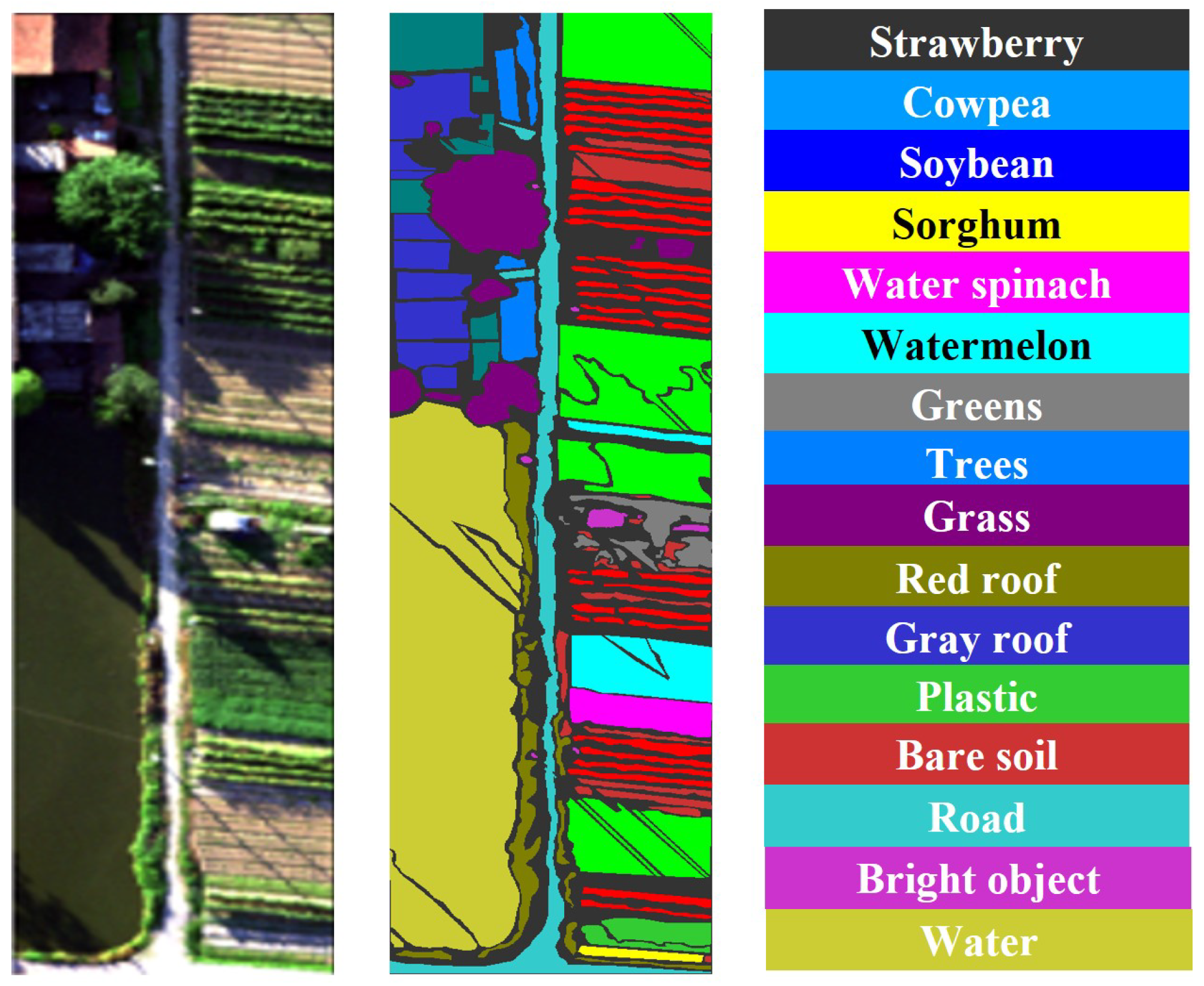
To comprehensively evaluate the performance of the proposed BiMambaHSI model, we conducted extensive experiments using five publicly available datasets that cover diverse characteristics: Pavia University [25], Houston [26], Indian Pines [27], WHU-Hi-HanChuan [28,29], and WHU-Hi-LongKou [28,29]. These datasets exhibit significant differences in spatial resolution, spectral characteristics, scene complexity, and category distribution. We provided an overview of their ground-truth annotations. The original hyperspectral image, the corresponding land-cover categories, and their spatial distributions are illustrated in Figure 1, Figure 2, Figure 3, Figure 4 and Figure 5. Furthermore, the number of samples for each class is summarized in

Table 1. Number of training and testing samples for five datasets.

Pavia University				Houston				WHU-Hi-HanChuan
Class		Number of Sample		Class		Number of Sample		Class		Number of Sample
No.	Name	Train	Test	No.	Name	Train	Test	No.	Name	Train	Test
1	Asphalt	66	6565	1	Grass healthy	63	1188	1	Paddy field	2237	42,498
2	Meadows	186	18,463	2	Grass stressed	63	1191	2	Irrigated field	1138	21,615
3	Gravel	21	2078	3	Grass synthetic	35	662	3	Dry cropland	514	9773
4	Trees	31	3033	4	Tree	62	1182	4	Garden plot	268	5085
5	Painted metal sheets	13	1332	5	Soil	62	1180	5	Arbor forest	60	1140
6	Bare Soil	50	4979	6	Water	16	309	6	Shrub land	227	4306
7	Bitumen	13	1317	7	Residential	63	1205	7	Natural meadow	295	5608
8	Self-Blocking Bricks	37	3645	8	Commercial	62	1182	8	Artificial meadow	899	17,079
9	Shadows	9	938	9	Road	63	1189	9	Industrial land	473	8996
Indian Pines				10	Highway	61	1166	10	Urban residential	526	9990
Class		Number of Sample		11	Railway	62	1173	11	Rural residential	846	16,065
No.	Name	Train	Test	12	Parking Lot 1	62	1171	12	Traffic land	184	3495
1	Alfalfa	5	41	13	Parking Lot 2	23	446	13	River	456	8660
2	Corn-notill	143	1285	14	Tennis Court	21	407	14	Lake	928	17,632
3	Corn-mintill	83	747	15	Running Track	33	627	15	Pond	57	1079
4	Corn	24	213	WHU-Hi-LongKou				16	Bare land	3770	71,631
5	Grass-pasture	48	435	Class		Number of Sample
6	Grass–trees	73	657	No.	Name	Train	Test
7	Grass–pasture–mowed	3	25	1	Corn	34	34,477
8	Hay-windrowed	48	430	2	Cotton	8	8366
9	Oats	2	18	3	Sesame	3	3028
10	Soybean-notill	97	875	4	Broad-leaf soybean	63	63,149
11	Soybean-mintill	246	2209	5	Narrow-leaf soybean	4	4147
12	Soybean-clean	59	534	6	Rice	11	11,843
13	Wheat	21	184	7	Water	67	66,989
14	Woods	127	1138	8	Roads and houses	7	7117
15	Buildings–Grass–Trees–Drives	39	347	9	Mixed weed	5	5224
16	Stone–Steel–Towers	10	83

, offering a clear view of the data composition across different categories.

2.1.1. Houston Dataset

The Houston dataset was collected by the AVIRIS sensor over the University of Houston campus, USA. It consists of 349 × 1905 pixels with 144 spectral bands covering 380–2500 nm. Fifteen classes are annotated, including buildings, roads, trees, and grass. This dataset is more challenging due to its large area, high intra-class variability, and shadow effects.

2.1.2. Indian Pines Dataset

The Indian Pines dataset, captured by AVIRIS over northwestern Indiana, contains 145 × 145 pixels and 200 spectral bands (after water-band removal). It covers agricultural fields with 16 land-cover classes, mostly crops, soil, and forest. Due to high spectral similarity among vegetation categories, it is often used to test spectral discrimination ability.

2.1.3. WHU-Hi-HanChuan Dataset

The WHU-Hi-HanChuan dataset, also captured by ZY-1, represents a suburban area in Hanchuan, China. It consists of 480 × 300 pixels with 270 spectral bands after preprocessing. Nine categories are defined, primarily vegetation, bare soil, and residential regions. This dataset features homogeneous agricultural scenes and smooth spatial transitions, suitable for testing spatial consistency.

2.1.4. WHU-Hi-LongKou Dataset

The WHU-Hi-Longkou dataset was acquired by the ZY-1 hyperspectral sensor over Longkou, China. It has 550 × 400 pixels and 270 spectral bands, covering urban and coastal areas. Ten land-cover types are annotated, including buildings, roads, vegetation, and water. It serves as a high-resolution benchmark with complex spatial textures and spectral diversity.

2.2. Preliminaries

In recent years, Structured State Space Models (SSMs) have attracted widespread attention in deep learning. Models of this type, such as S4 and Mamba, inherit the principles of classical state—space systems and have demonstrated great potential in sequence modeling. The core idea is to use hidden state variables $h^{\prime }\left(t\right)\in {\mathbb{R}}^N$ to model a one-dimensional input sequence $x\left(t\right)\in \mathbb{R}$, mapping it to an output $y\left(t\right)\in \mathbb{R}$, thereby establishing the dynamic relationship between input and output. This process can be described by the following linear ordinary differential equation (ODE)

$$\begin{array}{cc}\hfill h^{\prime }\left(t\right)& =\mathbf{A}h\left(t\right)+\mathbf{B}x\left(t\right),\hfill \\ \hfill y\left(t\right)& =\mathbf{C}h\left(t\right),\hfill \end{array}$$

(1)

where $\mathbf{A}\in {\mathbb{R}}^{N\times N}$ is the state matrix, $\mathbf{B}\in {\mathbb{R}}^{N\times 1}$, and $\mathbf{C}\in {\mathbb{R}}^{1\times N}$ are the projection parameters. To handle discrete data such as images and natural language, the continuous form of state space systems needs to be discretized. To this end, S4 and Mamba introduce a time-scale parameter $\Delta$ and apply a fixed discretization rule to transform the continuous parameters $\mathbf{A}$ and $\mathbf{B}$ into their discrete counterparts $\overline{\mathbf{A}}$ and $overline\mathbf{B}$. The most commonly used method is the Zero-Order Hold (ZOH), defined as the following:

$$\begin{array}{cc}\hfill \overline{\mathbf{A}}& =exp(\Delta \mathbf{A}),\hfill \\ \hfill \overline{\mathbf{B}}& ={(\Delta \mathbf{A})}^{-1}\left(exp(\Delta \mathbf{A})-\mathbf{I}\right)·\Delta \mathbf{B}.\hfill \end{array}$$

(2)

After discretization, SSM-based models can be computed in the recurrence form, which updates the hidden state step by step as follows:

$$\begin{array}{cc}\hfill h_t& =\overline{\mathbf{A}}{h}_{t-1}+\overline{\mathbf{B}}{x}_t,\hfill \\ \hfill y_t& =\mathbf{C}{h}_t\hfill \end{array}.$$

(3)

Alternatively, it can be expressed in the convolutional form, representing the entire sequence as a convolution with the system kernel as the following:

$$\begin{array}{cc}\hfill \mathbf{K}& =\left(\mathbf{C}\overline{\mathbf{B}},\mathbf{C}\overline{\mathbf{A}}\overline{\mathbf{B}},\dots ,\mathbf{C}{\overline{\mathbf{A}}}^{L-1}\overline{\mathbf{B}}\right),\hfill \\ \hfill y& =x·\mathbf{K},\hfill \end{array}$$

(4)

where L denotes the sequence length, which determines the expansion scale of the convolution kernel $\mathbf{K}$. This transition from continuous to discrete representation enables SSMs to retain theoretical modeling capacity while achieving linear-time complexity for long sequence modeling, laying the foundation for the wide adoption of S4 and Mamba in deep learning.

2.3. BiMambaHSI Overview

Our proposed framework, termed BiMambaHSI, is illustrated in Figure 6. The entire architecture is composed of three main components: (i) an Embedding Layer that produces multi-scale spectral—spatial embeddings from hyperspectral patches, (ii) a set of joint spectral—spatial bidirectional gated Mamba Encoders,which form the core of our framework and incorporate the newly designed spatial—spectral Mamba block (SSMB) to explicitly enhance bidirectional spectral—spatial modeling, and (iii) a Multi-scale Classification Head that integrates the encoder multi-scale outputs for final prediction. By introducing the JGM together with SSMB, BiMambaHSI not only captures long-range dependencies with linear complexity but also alleviates the limitations of insufficient spectral relation modeling and unidirectional sequence processing.

(1) Embedding Layer: Given an input hyperspectral image $\mathbf{I}\in {\mathbb{R}}^{H\times W\times C}$, we first apply principal component analysis (PCA) to reduce spectral redundancy. Pixel-centered patches of size $N\times N\times C$ are then extracted and passed through multi-scale 3D convolutional branches. Each branch corresponds to one scale s and consists of a convolution layer, batch normalization, and SiLU activation. The embedding feature on scale s is formulated as the following:

$${\mathbf{E}}_s=\mathrm{SiLU}\left(\mathrm{BN}3\mathrm{D}\left({\mathrm{Conv}3\mathrm{D}}_s\left({\mathbf{I}}_{patch}\right)\right)\right),s=1,2,\dots ,S,$$

(5)

where S denotes the number of scales. The outputs $\{{\mathbf{E}}_1,{\mathbf{E}}_2,\dots ,{\mathbf{E}}_S\}$ are then fed into the gated BiMamba encoders. In our BiMambaHSI framework, we specifically adopt $S=2$ scales, corresponding to convolution kernels of size $1\times 1$ and $3\times 3$, in order to capture both fine-grained spectral cues and broader spatial—spectral dependencies.

(2) Joint spectral—spatial Bidirectional Gated Mamba encoder: Each embedding ${\mathbf{E}}_s$ is processed by a gated BiMamba encoder, which constitutes the core innovation of our framework. Additionally, the encoder employs the proposed SSMB as its basic unit as follows:

$${\mathbf{H}}_s=\mathrm{Encoder}\left({\mathbf{E}}_s\right).$$

(6)

where ${\mathbf{H}}_s$ denotes the bidirectionally enhanced representation for scale s. This design allows the encoder to overcome the limitations of traditional Mamba-based models by explicitly exploiting both spectral relationships and spatial—spectral dependencies in a bidirectional manner.

(3) Multi-scale Classification Head: The outputs from all encoders are aggregated for classification. Specifically, the features $\{{\mathbf{H}}_1,{\mathbf{H}}_2,\dots ,{\mathbf{H}}_S\}$ are summed, followed by average pooling and reshaping to form the final representation as the following:

$$\mathbf{Z}=\mathrm{Reshape}\left(\mathrm{AvgPooling}\left(\sum _{s=1}^S{\mathbf{H}}_s\right)\right).$$

(7)

Finally, a linear classifier maps $\mathbf{Z}$ to the predicted class labels as follows:

$$\widehat{y}=\mathrm{Classifier}\left(\mathbf{Z}\right).$$

(8)

This multiscale fusion design allows BiMambaHSI to integrate complementary spectral and spatial cues across different receptive fields, thereby improving classification accuracy on complex hyperspectral scenes.

2.4. Joint Spectral—Spatial Bidirectional Gated Mamba (JGM) Encoder

The JGM encoder extends the unidirectional sequence modeling framework of Mamba by introducing forward and backward state propagation, enabling more explicit modeling of spectral—spatial interactions. Unlike existing approaches (e.g., Hypersigma [12]), our encoder does not separate spectral and spatial features at the very beginning. Instead, it unifies hyperspectral patches into a sequence of tokens, ensuring that the correlations across both spectral and spatial dimensions can be jointly captured from the start. The underlying module employed in this encoder is the spatial—spectral Mamba block (SSMB), which extends Mamba for hyperspectral data; its detailed design will be presented in Section 2.4. This strategy allows the encoder to explicitly model cross-dimensional relationships rather than treating spectra and space in isolation. Furthermore, to overcome the limitation of unidirectional processing, we introduce a bidirectional mechanism, where each sequence is modeled in both forward and backward directions, Given the embedding feature ${\mathbf{E}}_s\in {\mathbb{R}}^{L\times L\times D}$, we first apply normalization and projection to obtain a latent representation ${\mathbf{Z}}_s$ as follows:

$${\mathbf{Z}}_s=\mathrm{Proj}\left(\mathrm{Norm}\left({\mathbf{E}}_s\right)\right).$$

(9)

In parallel, we do not create a separate gating branch. Instead, the projected tensor ${\mathbf{Z}}_s\in {\mathbb{R}}^{L\times L\times 2D}$ is split along the channel dimension into a content part and a gating part as follows:

$${\mathbf{Z}}_s=\left[{\mathbf{Z}}_s^{\left(c\right)},{\mathbf{Z}}_s^{\left(g\right)}\right],{\mathbf{Z}}_s^{\left(c\right)},{\mathbf{Z}}_s^{\left(g\right)}\in {\mathbb{R}}^{L\times L\times D}$$

(10)

where the input-dependent gating weight is computed from the gating part via a SiLU nonlinearity followed by a sigmoid:

$${\mathbf{G}}_s=\sigma \left(\mathrm{SiLU}\left({\mathbf{Z}}_s^{\left(g\right)}\right)\right).$$

(11)

The content part ${\mathbf{Z}}_s^{\left(c\right)}$ is fed into the SSMB, while ${\mathbf{G}}_s$ is later used to adaptively fuse the forward and backward representations. With the split representation, the content features ${\mathbf{Z}}_s^{\left(c\right)}$ are processed by the SSMB in both forward and backward directions, yielding two complementary representations ${\mathbf{H}}_s^f$ and ${\mathbf{H}}_s^b$. To alleviate the limitation of unidirectional modeling, the final output of the encoder is obtained by adaptively fusing these two representations under the control of the gating weight ${\mathbf{G}}_s$ as follows:

$${\mathbf{H}}_s={\mathbf{G}}_s\odot {\mathbf{H}}_s^f+(1-{\mathbf{G}}_s)\odot {\mathbf{H}}_s^b,$$

(12)

where ⊙ denotes element-wise multiplication. This formulation allows the encoder to explicitly integrate spectral–spatial dependencies while simultaneously mitigating the shortcomings of single-directional processing. As a result, the proposed JGM encoder is able to capture richer discriminative representations tailored for hyperspectral image classification.

2.5. Spatial–Spectral Mamba Block (SSMB)

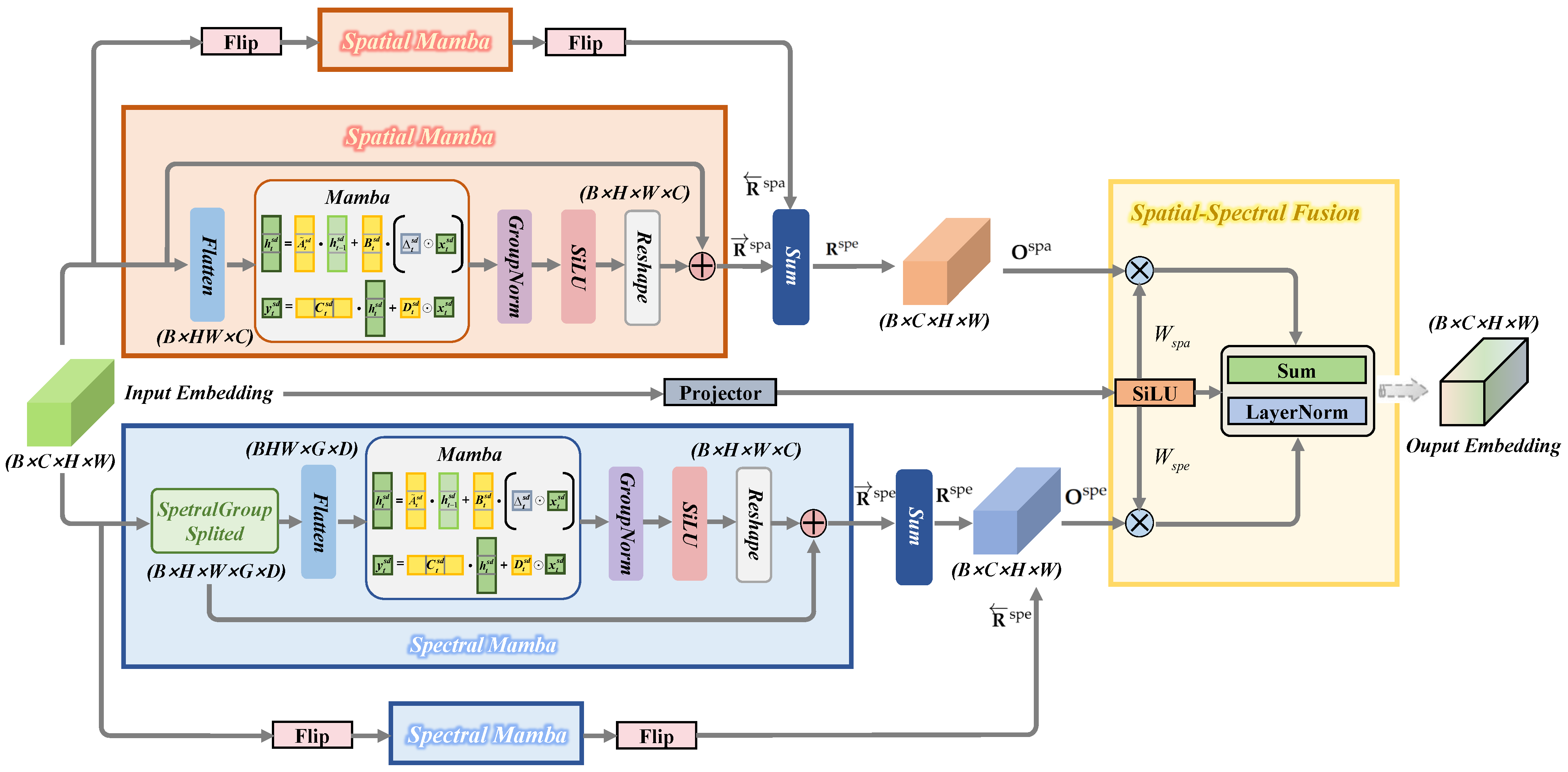
Building on the joint spectral—spatial tokenization achieved by the JGM encoder, the spatial—spectral Mamba block (SSMB) is designed to separately mine spatial and spectral cues while retaining bidirectional long-range modeling. As shown in Figure 7, SSMB splits the processing into two complementary branches: a spatial branch that specializes in spatial structures across patches and a spectral branch that focuses on spectral continuity across channels; both branches employ bidirectional Mamba to capture dependencies in two directions. Let $\mathbf{U}={\mathbf{Z}}_s^{\left(c\right)}\in {\mathbb{R}}^{L\times L\times D}$ denote the input to SSMB. For the spatial branch, the input $\mathbf{U}$ is first flattened into a sequence as follows:

$${\mathbf{H}}_F^{\mathrm{spa}}=\mathrm{Flatten}\left(\mathbf{U}\right).$$

(13)

where ${\mathbf{H}}_F^{\mathrm{spa}}\in {\mathbb{R}}^{L^2\times D}$. To capture bidirectional dependencies, we apply Mamba along both forward and reversed sequences, followed by group normalization and SiLU activation,

$$\begin{array}{cc}\hfill {\overrightarrow{\mathbf{R}}}^{\mathrm{spa}}& =\mathrm{SiLU}\left(\mathrm{GN}\left(\mathrm{Mamba}\left({\mathbf{H}}_F^{\mathrm{spa}}\right)\right)\right),\hfill \\ \hfill {\overleftarrow{\mathbf{R}}}^{\mathrm{spa}}& =\mathrm{Reverse}\left(\mathrm{SiLU}\left(\mathrm{GN}\left(\mathrm{Mamba}\left(\mathrm{Reverse}\left({\mathbf{H}}_F^{\mathrm{spa}}\right)\right)\right)\right)\right).\hfill \end{array}$$

(14)

One operates in the forward order, while the other processes the reversed sequence to capture backward dependencies. Their outputs are fused by a learnable gating weight ${\mathbf{g}}_{\mathrm{spa}}$, yielding

$${\mathbf{R}}^{\mathrm{spa}}={\mathbf{g}}_{\mathrm{spa}}·{\overrightarrow{\mathbf{R}}}^{\mathrm{spa}}+(1-{\mathbf{g}}_{\mathrm{spa}})·{\overleftarrow{\mathbf{R}}}^{\mathrm{spa}},$$

(15)

where ${\mathbf{g}}_{\mathrm{spa}}$ is a trainable parameter that adaptively balances the contributions of forward and backward spatial dependencies. The forward propagation captures spatial structural, while the backward propagation compensates the missing dependencies from the opposite direction. Compared to fixed summation, the gated design enables the model to adaptively adjust the weights of forward/backward information flows, thereby achieving greater robustness across datasets. Finally, the aggregated sequence is reshaped back into a spatial layout and added to the original input through a residual connection as follows:

$${\mathbf{O}}^{\mathrm{spa}}=\mathrm{Reshape}\left({\mathbf{R}}^{\mathrm{spa}}\right)+\mathbf{U}.$$

(16)

To enhance spectral information modeling, the spectral channels are first divided into G groups (each of size $M=D/G$). Let $\mathbf{U}\in {\mathbb{R}}^{L\times L\times D}$. We split channels and keep the spatial layout,

$${\mathbf{H}}_G^{\mathrm{spe}}=\mathrm{SplitSpectralGroup}\left(\mathbf{U}\right)\in {\mathbb{R}}^{L\times L\times G\times M}.$$

(17)

The spatial tokens are then flattened, producing a sequence per group along the intra-group spectral index,

$${\mathbf{H}}_F^{\mathrm{spe}}=\mathrm{Flatten}\left({\mathbf{H}}_G^{\mathrm{spe}}\right)\in {\mathbb{R}}^{L^2\times G\times M}.$$

(18)

Bidirectional Mamba is applied along the intra-group spectral dimension, followed by GN and SiLU; the backward pass reverses the G-axis as the following:

$$\begin{array}{cc}\hfill {\overrightarrow{\mathbf{R}}}^{\mathrm{spe}}& =\mathrm{SiLU}\left(\mathrm{GN}\left(\mathrm{Mamba}\left({\mathbf{H}}_F^{\mathrm{spe}}\right)\right)\right),\hfill \\ \hfill {\overleftarrow{\mathbf{R}}}^{\mathrm{spe}}& =\mathrm{Reverse}\left(\mathrm{SiLU}\left(\mathrm{GN}\left(\mathrm{Mamba}\left(\mathrm{Reverse}\left({\mathbf{H}}_F^{\mathrm{spe}}\right)\right)\right)\right)\right).\hfill \end{array}$$

(19)

The two directions are aggregated by summation. Unlike spatial structures, spectral bands are sampled in a strictly ordered continuous wavelength domain, and forward–backward propagation represents two complementary scanning directions along the same band axis. Since spectral continuity is globally smooth and less variable than spatial textures, equal-weight aggregation provides a stable and parameter-free fusion strategy. This allows the model to integrate long-range spectral correlations without introducing extra learnable coefficients, preserving pure SSM linear complexity as the following:

$${\mathbf{R}}^{\mathrm{spe}}={\overrightarrow{\mathbf{R}}}^{\mathrm{spe}}+{\overleftarrow{\mathbf{R}}}^{\mathrm{spe}}.$$

(20)

Finally, the sequence is reshaped back, spectral groups are merged, and a residual connection is added,

$${\mathbf{O}}^{\mathrm{spe}}=\mathrm{Reshape}\left({\mathbf{R}}^{\mathrm{spe}}\right)+\mathbf{U}.$$

(21)

This branch explicitly captures bidirectional dependencies among principal component channels within each spectral group and complements the spatial branch. Finally, the outputs from the spatial and spectral branches are integrated by a lightweight fusion module. Given the input embedding $\mathbf{U}$, two fusion weights are first computed through a shared projection followed by a SiLU activation as the following:

$$[{\mathbf{W}}_{\mathrm{spa}},{\mathbf{W}}_{\mathrm{spe}}]=\mathrm{SiLU}\left(\mathrm{Proj}\left(\mathbf{U}\right)\right).$$

(22)

The spatial and spectral outputs ${\mathbf{W}}^{\mathrm{spa}},{\mathbf{W}}^{\mathrm{spe}}\in {\mathbb{R}}^{L\times L\times D}$ are then combined in an adaptive manner as follows:

$${\mathbf{H}}_{\mathrm{fus}}={\mathbf{W}}_{\mathrm{spa}}·{\mathbf{O}}^{\mathrm{spa}}+{\mathbf{W}}_{\mathrm{spe}}·{\mathbf{O}}^{\mathrm{spe}}.$$

(23)

A normalization layer is subsequently applied to stabilize training as the following:

$$\mathbf{O}=\mathrm{LayerNorm}\left({\mathbf{H}}_{\mathrm{fus}}\right).$$

(24)

Through this design, the model learns to emphasize spatial or spectral representations depending on the input, enabling adaptive feature integration.

3. Results

3.1. Evaluation Indicators

We evaluated the proposed method using three widely adopted metrics in hyperspectral image classification: overall accuracy (OA), average accuracy (AA), and the Kappa coefficient ($\kappa$). These metrics complement each other by characterizing classification performance from different perspectives. Let the total number of test samples be N, the number of land-cover classes be C, and the confusion matrix be denoted as $\mathbf{M}\in {\mathbb{R}}^{C\times C}$, where each entry $M_{ij}$ represents the number of samples belonging to class i that are misclassified as class j.

• Overall Accuracy (OA): This metric measures the ratio of correctly classified pixels to the total number of test pixels, and it is referred to as the overall accuracy (OA) and defined as the following:

  $$\mathrm{OA}={\displaystyle \frac{{\sum }_{i=1}^C{M}_{ii}}{N}}.$$

  (25)
• Average Accuracy (AA): AA computes the average classification accuracy across all classes, assigning equal importance to each class regardless of its sample size. This ensures a more balanced evaluation of classification performance over all categories. The definition of AA is given as the following:

  $$\mathrm{AA}={\displaystyle \frac{1}{C}}\sum _{i=1}^C{\displaystyle \frac{M_{ii}}{{\sum }_{j=1}^C{M}_{ij}}}.$$

  (26)
• Kappa Coefficient ($\kappa$): The Kappa coefficient quantifies the level of agreement between the predicted classification results and the ground truth, while accounting for the agreement that may occur by chance. It is formulated as follows:

  $$\kappa ={\displaystyle \frac{N{\sum }_{i=1}^C{M}_{ii}-{\sum }_{i=1}^C\left({\sum }_{j=1}^C{M}_{ij}·{\sum }_{j=1}^C{M}_{ji}\right)}{N^2-{\sum }_{i=1}^C\left({\sum }_{j=1}^C{M}_{ij}·{\sum }_{j=1}^C{M}_{ji}\right)}}.$$

  (27)

3.2. Experimental Setup

To ensure fair comparisons and reproducibility, all experiments were implemented within a unified framework using a single NVIDIA RTX 4090 GPU and a 14th Gen Intel Core CPU under PyTorch 2.1. Following the common practice in previous studies [9,11], we applied PCA to each hyperspectral cube for spectral dimensionality reduction. Specifically, the number of retained components was set to 15 for Pavia University, 17 for Houston, 19 for Indian Pines, and 14 for both WHU-Hi-Hanchuan and WHU-Hi-LongKou. For a fair comparison with Hypersigma, which requires pretrained weights, we followed its setting and uniformly fixed the number of PCA components to 33.

During training, all models were optimized using the AdamW optimizer for 200 epochs, with an initial learning rate of $1\times {10}^{-3}$ and weight decay set to $0.005$. The learning rate adjustment employed a cosine-annealing scheduler, with a batch size of 128. These training hyperparameters were determined through preliminary experiments to ensure stable and efficient convergence across all datasets.

The training sample proportions for each dataset are shown in Table 1. The Pavia University dataset training set contains 1% of samples from each category. The training sets for the Houston and WHU-Hi-HanChuan datasets each contain 5% of samples per category. The Indian Pines dataset training set contains 10% of samples per category; The WHU-Hi-LongKou dataset contains 0.1% of samples per category. These challenging small-sample-size settings were designed to rigorously test the models’ generalization capabilities. The remaining samples in each dataset were used for testing.

3.3. Ablation Analysis

To analyze the contributions of individual modules, as shown in

Table 2. The ablation performance of different datasets.

Datasets	Base	JGM		SSMB			BiMambaHSI
		Sum	Gate	Spatial	Spectral	Spatial + Spectral
Pavia University	95.29 ± 0.71	95.36 ± 0.23	95.68 ± 0.68	95.87 ± 0.36	95.76 ± 0.24	96.14 ± 0.32	97.90 ± 0.11
Houston	96.75 ± 0.96	96.97 ± 0.57	97.08 ± 0.93	97.13 ± 0.26	97.30 ± 0.41	97.47 ± 1.04	97.92 ± 0.17
Indian Pines	97.83 ± 0.21	97.89 ± 0.62	98.01 ± 1.37	98.19 ± 0.86	98.17 ± 0.56	98.56 ± 1.10	99.02 ± 0.11
WHU-Hi-HanChuan	95.01 ± 0.32	95.37 ± 0.54	95.99 ± 0.21	96.02 ± 0.47	95.99 ± 0.70	96.52 ± 0.63	97.92 ± 0.27
WHU-Hi-LongKou	96.86 ± 0.45	96.96 ± 0.83	97.24 ± 1.08	97.76 ± 1.06	97.94 ± 0.79	98.27 ± 1.61	99.54 ± 0.03

, we conducted ablations focusing on the gated fusion in JGM and the dual-branch structure in SSMB.

• JGM fusion mechanism. Replacing gated fusion with simple summation yielded only slight improvement over the base model. With learnable gating, the accuracy increased more noticeably on all datasets (e.g., from 95.36% to 95.68% on PaviaU and from 96.97% to 97.08% on Houston), indicating that adaptive weighting provides more effective spectral—spatial integration.
• SSMB dual-branch structure. Spatial-only and spectral-only variants resulted in reduced accuracy, showing that both modalities contribute complementary information. For example, on Houston, spatial-only and spectral-only variants achieved 97.13% and 97.30%, while the dual-branch version reached 97.47%. Similar patterns appeared on other datasets.

With both components enabled, BiMambaHSI obtained the highest accuracy across datasets. These results suggested that performance gains came from explicit bidirectional spectral—spatial modeling with adaptive fusion, rather than increased model size.

3.4. Classification Performance

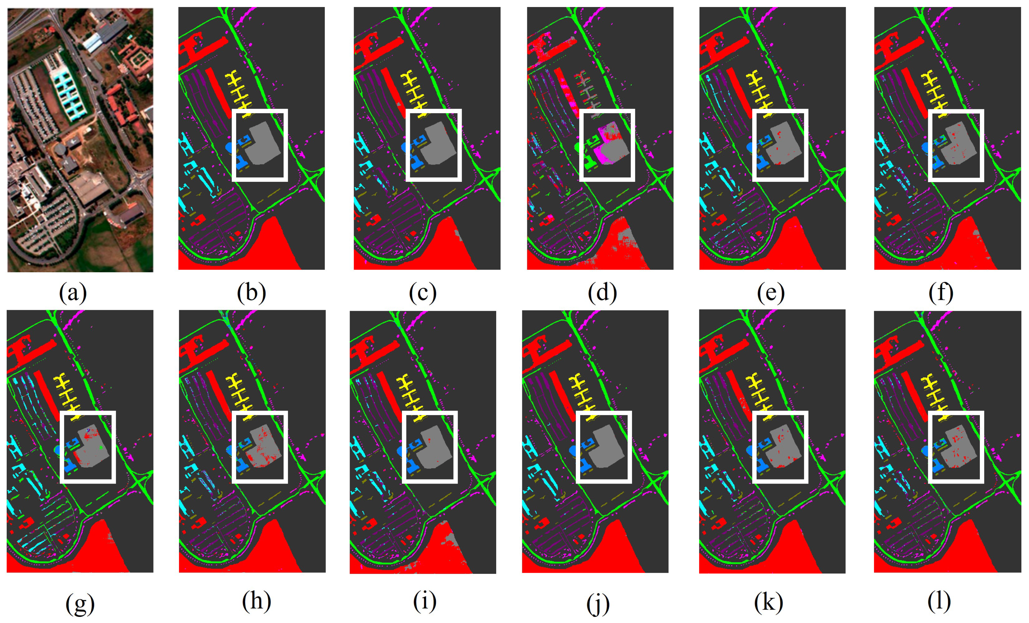
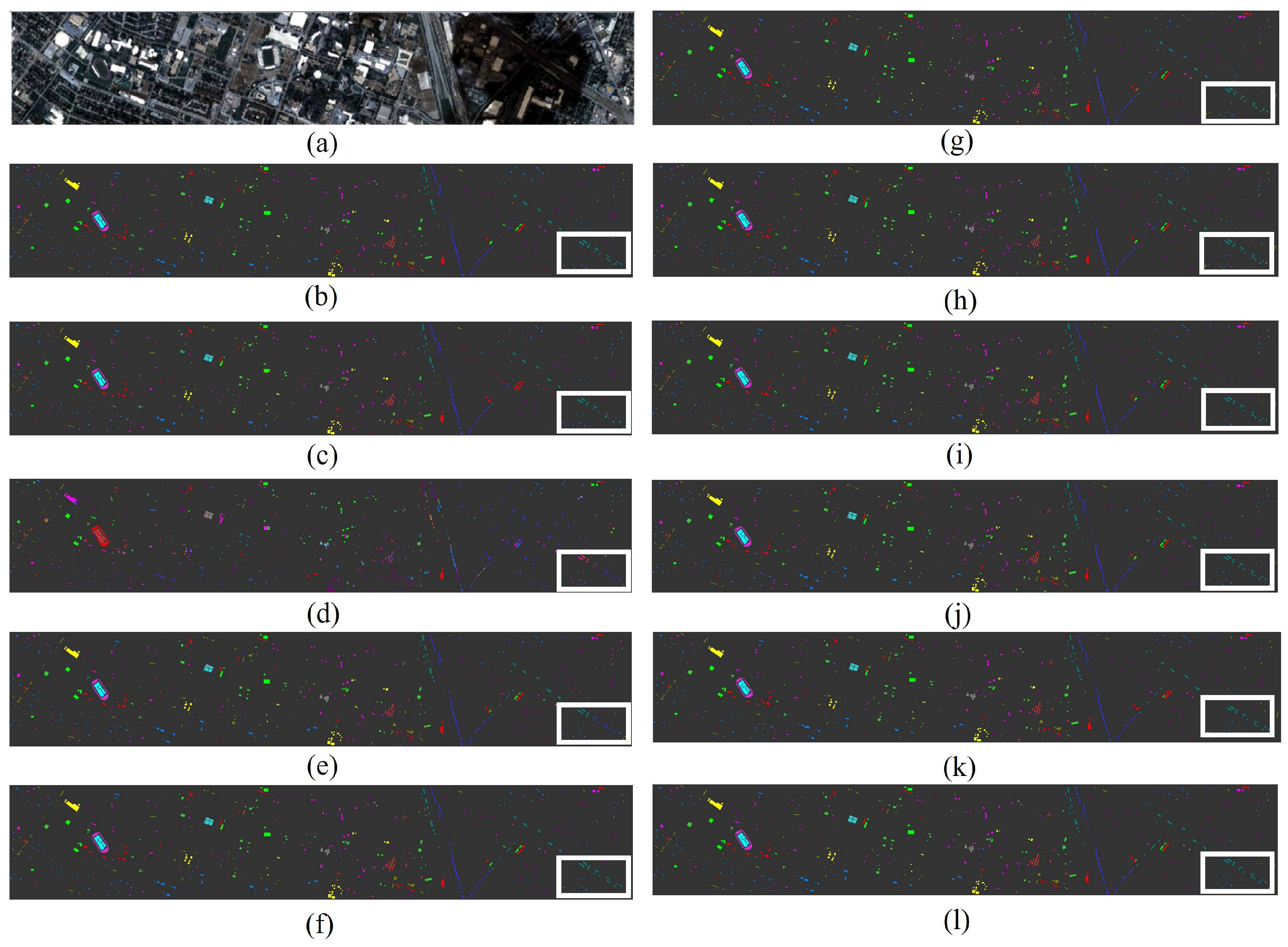
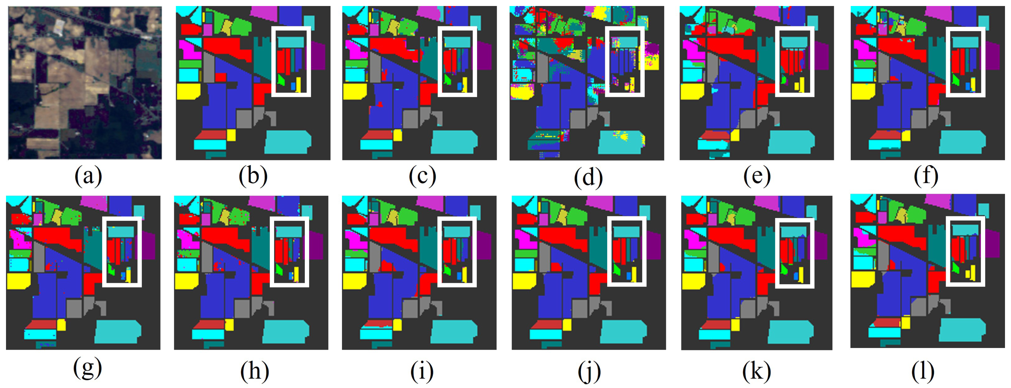
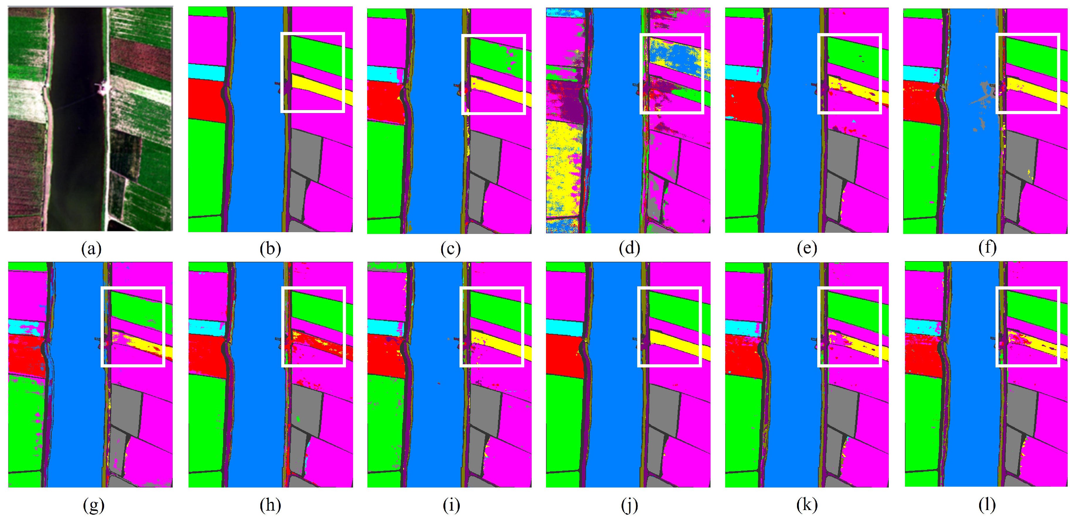
To comprehensively evaluate the effectiveness of the proposed method, we conducted experiments on five widely used hyperspectral datasets. We selected several representative hyperspectral classification models as comparison methods, including GSCNet [14], HyperSIGMA [12], Lite-HCNNet [11], MSDAN [9], SimpoolFormer [30], SpectralFormer [13], SSFTT [31], MambaHSI [20], and HGMamba [21], which can demonstrate performance differences from various perspectives. Detailed quantitative results are summarized in

Table 3. The classification performance of different methods for the Pavia University dataset.

No.	GSCNet [14]	Hyper-Sigma [12]	Lite-HCNnet [11]	MSDAN [9]	Simpool-Former [30]	Spetral-Former [13]	SSFTT [31]	Mamba-HSI [20]	HG-Mamba [21]	Ours
1	97.65 ± 0.65	97.08 ± 1.08	98.26 ± 0.77	95.01 ± 1.56	91.41 ± 2.53	94.25 ± 1.17	96.00 ± 1.25	96.37 ± 1.08	94.71 ± 0.81	99.07 ± 0.44
2	99.73 ± 0.24	99.39 ± 0.32	99.79 ± 0.13	99.38 ± 0.31	98.66 ± 0.46	99.27 ± 0.25	98.88 ± 0.68	99.43 ± 0.73	99.79 ± 0.54	99.85 ± 0.09
3	90.11 ± 9.80	75.44 ± 5.63	88.79 ± 1.99	87.07 ± 2.25	77.26 ± 5.61	79.00 ± 3.36	81.75 ± 3.56	85.23 ± 2.09	76.80 ± 2.03	83.92 ± 1.73
4	95.26 ± 1.64	89.49 ± 2.19	93.12 ± 1.64	90.85 ± 2.03	82.02 ± 3.62	87.02 ± 2.90	93.12 ± 2.25	91.30 ± 1.67	86.88 ± 1.99	93.72 ± 0.96
5	97.78 ± 2.16	99.70 ± 0.23	99.35 ± 0.27	98.32 ± 1.29	99.25 ± 1.02	99.43 ± 0.72	99.98 ± 0.04	97.90 ± 0.33	99.17 ± 0.17	99.85 ± 0.26
6	91.70 ± 6.52	93.08 ± 4.78	98.58 ± 0.81	98.15 ± 1.75	87.99 ± 1.19	97.25 ± 0.51	92.90 ± 2.83	94.98 ± 1.54	94.32 ± 1.06	99.76 ± 0.17
7	84.59 ± 3.19	75.28 ± 13.38	97.71 ± 2.00	98.40 ± 0.82	88.75 ± 3.68	83.75 ± 4.66	89.84 ± 4.23	96.13 ± 2.69	88.08 ± 3.18	95.78 ± 1.50
8	95.24 ± 3.75	77.88 ± 6.17	91.88 ± 1.56	89.75 ± 4.61	78.17 ± 6.88	86.61 ± 4.17	88.55 ± 3.84	86.36 ± 2.56	90.04 ± 1.84	96.32 ± 1.61
9	97.78 ± 1.20	93.32 ± 4.15	99.89 ± 0.11	89.01 ± 5.22	89.37 ± 7.86	97.29 ± 1.64	99.34 ± 0.83	95.84 ± 3.96	97.23 ± 4.11	92.27 ± 4.23
OA(%)	96.7 ± 0.79	93.66 ± 0.78	97.64 ± 0.29	96.22 ± 0.61	91.78 ± 0.47	94.77 ± 0.30	95.35 ± 0.55	95.8 ± 0.20	95.03 ± 0.17	97.90 ± 0.11
AA(%)	94.42 ± 1.30	88.85 ± 1.51	96.38 ± 0.45	93.9 ± 1.29	88.1 ± 0.57	91.54 ± 0.60	93.37 ± 0.52	93.73 ± 0.22	91.89 ± 0.20	95.62 ± 0.41
Kappa	95.61 ± 1.07	91.54 ± 1.04	96.86 ± 0.38	94.99 ± 0.82	89.01 ± 0.62	93.05 ± 0.40	93.82 ± 0.73	94.41 ± 0.46	93.36 ± 0.62	97.22 ± 0.15

,

Table 4. The classification performance of different methods for the Houston dataset.

No.	GSCNet [14]	Hyper-Sigma [12]	Lite-HCNnet [11]	MSDAN [9]	Simpool-Former [30]	Spetral-Former [13]	SSFTT [31]	Mamba-HSI [20]	HG-Mamba [21]	Ours
1	89.56 ± 6.50	95.32 ± 1.91	91.65 ± 2.33	96.94 ± 0.75	95.77 ± 1.49	97.84 ± 0.37	98.10 ± 1.28	87.54 ± 1.84	95.29 ± 1.79	98.62 ± 1.01
2	94.98 ± 4.73	96.47 ± 1.30	98.55 ± 0.34	98.66 ± 0.80	98.54 ± 1.18	98.20 ± 0.33	99.13 ± 0.15	99.92 ± 0.31	99.24 ± 0.29	99.06 ± 0.20
3	99.76 ± 0.46	99.79 ± 0.13	99.86 ± 0.32	99.94 ± 0.08	100.0 ± 0.00	100.0 ± 0.00	99.94 ± 0.13	99.70 ± 0.61	99.70 ± 0.37	100.00 ± 0.00
4	90.59 ± 7.37	97.59 ± 1.36	98.83 ± 1.10	98.65 ± 0.62	98.21 ± 1.86	99.85 ± 0.20	99.81 ± 0.17	99.32 ± 1.03	97.12 ± 0.76	98.97 ± 1.36
5	99.36 ± 0.7	99.87 ± 0.21	98.65 ± 0.94	99.97 ± 0.08	99.85 ± 0.11	99.98 ± 0.04	99.83 ± 0.22	100.00 ± 0.00	100.00 ± 0.00	100.0 ± 0.00
6	88.48 ± 9.43	89.53 ± 5.04	84.66 ± 3.70	99.35 ± 0.91	94.04 ± 5.12	90.74 ± 0.88	96.31 ± 3.09	98.06 ± 2.19	100.00 ± 0.00	97.80 ± 2.72
7	91.55 ± 1.74	92.42 ± 1.80	91.75 ± 1.60	95.42 ± 1.61	91.60 ± 3.73	92.51 ± 3.17	94.84 ± 1.94	93.03 ± 1.09	93.28 ± 1.41	93.14 ± 0.71
8	84.35 ± 2.78	86.5 ± 1.76	73.69 ± 5.50	96.19 ± 0.98	92.78 ± 2.17	94.35 ± 1.21	93.00 ± 1.19	97.97 ± 1.22	95.94 ± 1.05	95.84 ± 0.81
9	87.67 ± 4.29	79.74 ± 1.75	81.07 ± 5.66	94.84 ± 1.72	90.60 ± 4.00	96.81 ± 1.88	95.11 ± 0.69	96.38 ± 2.43	96.97 ± 2.90	97.34 ± 0.50
10	92.13 ± 4.79	91.1 ± 1.38	94.01 ± 1.54	97.22 ± 1.04	98.08 ± 0.94	99.33 ± 0.52	95.75 ± 1.09	99.40 ± 1.17	95.54 ± 1.75	99.21 ± 0.76
11	88.53 ± 2.53	97.67 ± 1.22	89.30 ± 4.25	98.88 ± 0.92	94.10 ± 6.38	98.13 ± 0.87	97.87 ± 1.17	91.30 ± 3.02	88.32 ± 2.54	98.71 ± 0.70
12	89.5 ± 4.07	94.44 ± 3.34	83.75 ± 5.71	96.09 ± 0.82	95.30 ± 2.94	98.23 ± 0.72	98.36 ± 0.90	97.10 ± 0.09	97.27 ± 0.19	98.91 ± 0.48
13	81.03 ± 10.11	87.00 ± 4.73	86.29 ± 5.87	94.8 ± 4.31	52.42 ± 13.64	73.32 ± 4.35	93.41 ± 2.92	95.74 ± 2.77	91.26 ± 3.04	89.28 ± 2.32
14	97.79 ± 2.78	100.0 ± 0.00	98.54 ± 1.07	99.75 ± 0.17	99.80 ± 0.44	99.51 ± 0.46	99.31 ± 0.27	100.00 ± 0.00	100.00 ± 0.00	99.70 ± 0.20
15	98.95 ± 1.15	99.97 ± 0.07	99.54 ± 0.47	100.0 ± 0.00	99.23 ± 0.61	99.84 ± 0.28	99.42 ± 0.63	100.00 ± 0.00	100.00 ± 0.00	99.81 ± 0.26
OA(%)	91.44 ± 0.24	93.64 ± 0.22	90.99 ± 0.67	97.56 ± 0.22	94.59 ± 0.51	96.88 ± 0.49	97.33 ± 0.39	96.65 ± 0.27	96.32 ± 0.53	97.92 ± 0.17
AA(%)	91.62 ± 0.72	93.83 ± 0.24	91.34 ± 0.74	97.78 ± 0.31	93.35 ± 0.79	95.91 ± 0.49	97.35 ± 0.56	97.03 ± 0.21	96.66 ± 0.49	97.76 ± 0.30
Kappa	90.74 ± 0.26	93.13 ± 0.24	90.26 ± 0.72	97.36 ± 0.24	94.15 ± 0.55	96.63 ± 0.53	97.11 ± 0.42	96.38 ± 0.50	96.02 ± 0.37	97.75 ± 0.19

,

Table 5. The classification performance of different methods for the Indian Pines dataset.

No.	GSCNet [14]	Hyper-Sigma [12]	Lite-HCNnet [11]	MSDAN [9]	Simpool-Former [30]	Spetral-Former [13]	SSFTT [31]	Mamba-HSI [20]	HG-Mamba [21]	Ours
1	99.46 ± 1.01	95.61 ± 4.36	99.46 ± 1.21	98.38 ± 2.42	90.81 ± 10.22	98.38 ± 1.48	89.52 ± 7.64	90.91 ± 2.37	97.73 ± 2.40	98.92 ± 1.48
2	94.98 ± 0.78	90.46 ± 1.58	96.49 ± 1.27	97.52 ± 0.76	92.81 ± 0.69	93.21 ± 1.19	97.48 ± 0.38	95.65 ± 0.91	95.50 ± 0.79	97.88 ± 0.87
3	97.59 ± 2.08	95.82 ± 1.86	99.49 ± 0.38	98.55 ± 0.57	95.24 ± 1.25	97.74 ± 0.74	97.09 ± 0.91	98.99 ± 0.26	97.97 ± 0.73	98.28 ± 0.46
4	98.32 ± 1.26	93.71 ± 1.87	98.42 ± 3.53	99.68 ± 0.47	86.84 ± 3.63	91.89 ± 1.60	97.16 ± 2.04	93.78 ± 2.15	95.56 ± 2.09	100.00 ± 0.00
5	96.79 ± 1.84	93.93 ± 1.18	98.91 ± 0.64	97.82 ± 1.09	96.79 ± 1.03	94.71 ± 2.20	95.23 ± 0.74	100.00 ± 0.00	100.00 ± 0.00	99.58 ± 0.51
6	98.77 ± 0.99	99.03 ± 0.32	99.35 ± 0.59	98.94 ± 0.52	99.21 ± 0.58	99.83 ± 0.17	97.05 ± 0.78	98.70 ± 0.36	97.26 ± 0.52	99.32 ± 0.40
7	100.00 ± 0.00	80.0 ± 18.55	94.54 ± 3.80	99.93 ± 0.15	81.82 ± 14.37	98.18 ± 2.49	88.46 ± 6.08	92.59 ± 3.10	70.37 ± 3.47	100.00 ± 0.00
8	99.27 ± 1.36	100.00 ± 0.00	99.69 ± 0.47	99.69 ± 0.7	99.63 ± 0.54	100.00 ± 0.00	99.91 ± 0.20	100.00 ± 0.00	100.00 ± 0.00	100.00 ± 0.00
9	78.75 ± 19.06	45.56 ± 9.13	87.5 ± 17.68	87.50 ± 4.42	86.25 ± 6.85	97.5 ± 3.42	90.00 ± 7.24	73.68 ± 4.92	36.84 ± 8.78	100.00 ± 0.00
10	96.38 ± 1.34	91.98 ± 2.42	98.15 ± 1.91	98.79 ± 1.2	93.22 ± 1.11	95.55 ± 1.16	93.89 ± 1.43	97.62 ± 0.58	98.70 ± 0.31	98.79 ± 0.68
11	98.61 ± 0.38	97.31 ± 0.92	99.09 ± 0.27	98.83 ± 0.66	98.56 ± 0.48	98.68 ± 0.17	97.77 ± 0.46	98.28 ± 0.40	97.51 ± 0.23	99.85 ± 0.12
12	97.31 ± 1.54	89.17 ± 1.94	97.26 ± 1.31	95.92 ± 1.43	92.55 ± 3.12	95.11 ± 1.44	96.01 ± 2.25	92.90 ± 2.79	90.59 ± 2.47	95.96 ± 1.68
13	98.78 ± 2.73	99.14 ± 0.3	99.51 ± 0.67	100.00 ± 0.0	99.63 ± 0.33	100.0 ± 0.00	98.09 ± 1.57	97.44 ± 1.09	96.92 ± 1.38	100.00 ± 0.00
14	99.76 ± 0.20	99.86 ± 0.12	99.92 ± 0.13	99.84 ± 0.11	99.23 ± 0.36	99.21 ± 0.34	99.26 ± 0.27	99.00 ± 0.03	98.50 ± 0.07	99.98 ± 0.04
15	97.86 ± 0.96	97.46 ± 1.25	99.16 ± 0.85	99.48 ± 0.59	96.83 ± 1.92	97.35 ± 1.69	90.48 ± 2.07	93.19 ± 2.84	94.01 ± 2.57	99.68 ± 0.23
16	98.92 ± 1.13	79.29 ± 10.47	98.11 ± 1.54	96.49 ± 3.39	97.30 ± 1.91	94.86 ± 4.21	80.23 ± 2.10	64.77 ± 2.90	85.23 ± 4.03	91.62 ± 3.50
OA(%)	97.77 ± 0.19	95.3 ± 0.79	98.66 ± 0.44	98.62 ± 0.24	96.30 ± 0.41	97.14 ± 0.27	96.80 ± 0.21	97.17 ± 0.27	96.84 ± 0.44	99.02 ± 0.11
AA(%)	96.97 ± 1.36	90.52 ± 1.98	97.82 ± 0.94	97.92 ± 0.45	94.17 ± 1.59	97.01 ± 0.32	94.23 ± 1.28	92.97 ± 0.74	90.79 ± 0.98	98.74 ± 0.32
Kappa	97.46 ± 0.22	94.64 ± 0.9	98.47 ± 0.51	98.42 ± 0.28	95.78 ± 0.46	96.74 ± 0.31	96.35 ± 0.23	96.76 ± 0.42	96.38 ± 0.37	98.88 ± 0.13

,

Table 6. The classification performance of different methods for the WHU-Hi-HanChuan dataset.

No.	GSCNet [14]	Hyper-Sigma [12]	Lite-HCNnet [11]	MSDAN [9]	Simpool-Former [30]	Spetral-Former [13]	SSFTT [31]	Mamba-HSI [20]	HG-Mamba [21]	Ours
1	97.13 ± 1.53	97.62 ± 0.49	97.62 ± 0.48	97.93 ± 0.23	98.85 ± 1.23	98.32 ± 0.52	97.21 ± 1.05	97.64 ± 0.94	97.74 ± 1.03	99.22 ± 0.26
2	92.02 ± 2.91	95.27 ± 4.44	93.56 ± 1.16	94.96 ± 1.31	95.47 ± 3.95	94.95 ± 0.95	93.21 ± 1.55	90.90 ± 2.87	92.14 ± 1.33	96.97 ± 0.80
3	93.91 ± 4.79	95.58 ± 2.02	94.30 ± 3.36	95.78 ± 1.38	96.01 ± 3.30	97.00 ± 1.09	91.96 ± 2.30	95.83 ± 1.89	96.07 ± 1.02	97.91 ± 0.68
4	97.24 ± 1.38	99.33 ± 0.36	97.81 ± 0.43	98.79 ± 0.62	99.48 ± 1.45	98.31 ± 0.49	98.12 ± 0.74	98.84 ± 0.95	98.00 ± 1.22	99.24 ± 0.63
5	67.58 ± 14.66	66.75 ± 4.76	85.74 ± 5.67	76.0 ± 14.93	85.75 ± 9.58	90.28 ± 3.53	75.19 ± 8.21	91.14 ± 2.37	68.21 ± 4.98	91.74 ± 3.45
6	65.97 ± 5.30	67.91 ± 2.49	63.76 ± 7.02	73.56 ± 4.11	78.36 ± 10.43	68.04 ± 3.94	68.24 ± 6.49	72.16 ± 2.01	70.96 ± 2.09	88.33 ± 1.34
7	81.67 ± 12.06	89.16 ± 0.73	86.91 ± 7.36	87.75 ± 7.64	92.48 ± 3.60	92.66 ± 3.35	88.51 ± 1.33	91.69 ± 1.42	92.49 ± 1.08	96.56 ± 1.11
8	82.09 ± 4.25	90.43 ± 1.57	88.67 ± 3.02	89.93 ± 1.02	91.93 ± 4.50	89.74 ± 1.69	90.38 ± 2.80	89.73 ± 3.97	86.00 ± 2.01	96.16 ± 1.05
9	87.47 ± 2.96	89.12 ± 1.09	88.63 ± 3.58	88.86 ± 3.46	92.76 ± 3.26	90.71 ± 1.60	87.00 ± 2.04	89.34 ± 3.46	90.65 ± 2.70	96.51 ± 1.16
10	96.74 ± 2.68	87.64 ± 2.54	97.01 ± 1.77	98.12 ± 1.05	99.25 ± 1.42	98.64 ± 0.57	97.7 ± 0.55	98.49 ± 0.81	98.29 ± 0.49	99.15 ± 0.55
11	94.36 ± 2.99	97.09 ± 0.55	96.03 ± 1.50	96.17 ± 1.98	97.73 ± 1.90	95.35 ± 1.52	95.79 ± 2.56	98.07 ± 0.88	95.36 ± 3.07	98.92 ± 0.26
12	71.34 ± 19.12	94.31 ± 2.54	76.79 ± 8.41	82.59 ± 8.90	86.42 ± 6.44	89.98 ± 3.74	80.29 ± 5.77	88.96 ± 3.02	80.02 ± 4.91	93.19 ± 2.46
13	79.78 ± 10.53	88.41 ± 2.30	75.75 ± 6.65	77.44 ± 5.76	80.86 ± 6.76	78.47 ± 3.59	77.84 ± 0.79	83.72 ± 2.10	79.95 ± 2.38	89.74 ± 2.40
14	89.42 ± 4.53	97.59 ± 0.30	90.96 ± 1.50	90.80 ± 3.01	96.40 ± 2.98	94.28 ± 0.84	91.39 ± 0.76	96.74 ± 0.98	93.06 ± 1.23	96.65 ± 0.77
15	81.91 ± 7.29	96.07 ± 1.40	72.60 ± 10.81	84.06 ± 9.00	71.66 ± 22.84	68.12 ± 5.94	82.48 ± 4.21	84.06 ± 3.02	80.94 ± 3.10	95.54 ± 1.01
16	99.49 ± 0.53	99.59 ± 0.12	99.49 ± 0.15	99.53 ± 0.10	99.63 ± 0.08	99.72 ± 0.13	99.37 ± 0.22	99.48 ± 0.03	99.52 ± 0.04	99.88 ± 0.06
OA(%)	93.00 ± 0.64	97.78 ± 0.10	94.04 ± 0.24	94.78 ± 0.15	96.53 ± 0.64	95.37 ± 0.12	94.15 ± 0.17	95.39 ± 0.16	94.47 ± 0.19	97.92 ± 0.27
AA(%)	86.14 ± 2.20	95.66 ± 0.47	87.85 ± 0.83	89.52 ± 0.75	91.50 ± 0.71	90.29 ± 0.55	88.42 ± 0.86	91.67 ± 0.66	88.71 ± 0.65	95.98 ± 0.49
Kappa	91.80 ± 0.75	97.40 ± 0.12	93.02 ± 0.28	93.89 ± 0.18	95.76 ± 0.75	94.58 ± 0.14	93.15 ± 0.21	94.60 ± 0.41	93.52 ± 0.94	97.56 ± 0.32

and

Table 7. The classification performance of different methods for the WHU-Hi-LongKou dataset.

No.	GSCNet [14]	Hyper-Sigma [12]	Lite-HCNnet [11]	MSDAN [9]	Simpool-Former [30]	Spetral-Former [13]	SSFTT [31]	Mamba-HSI [20]	HG-Mamba [21]	Ours
1	99.86 ± 0.08	99.84 ± 0.04	99.97 ± 0.02	98.64 ± 0.57	99.66 ± 0.26	99.67 ± 0.13	99.76 ± 0.09	99.74 ± 0.10	99.42 ± 0.08	99.90 ± 0.11
2	99.08 ± 0.83	93.83 ± 4.44	96.68 ± 0.77	95.46 ± 1.87	83.04 ± 5.52	91.31 ± 4.96	97.90 ± 1.11	93.29 ± 1.43	91.67 ± 2.37	99.63 ± 0.12
3	95.86 ± 2.35	84.55 ± 7.00	95.66 ± 1.52	93.33 ± 5.06	91.51 ± 4.97	92.58 ± 1.87	94.38 ± 2.87	91.34 ± 2.09	87.27 ± 2.41	99.19 ± 0.68
4	99.39 ± 0.21	99.27 ± 0.36	99.40 ± 0.18	99.23 ± 0.24	97.84 ± 0.64	98.68 ± 0.32	99.20 ± 0.18	98.26 ± 0.21	98.67 ± 0.14	99.63 ± 0.12
5	88.90 ± 5.28	66.47 ± 4.76	81.28 ± 7.96	63.55 ± 8.08	72.61 ± 9.66	62.06 ± 8.81	70.08 ± 4.86	68.96 ± 4.07	69.37 ± 4.89	96.85 ± 0.85
6	99.57 ± 0.39	99.50 ± 0.38	99.33 ± 0.51	97.06 ± 2.28	98.77 ± 0.86	98.03 ± 1.10	99.71 ± 0.19	99.40 ± 0.04	99.06 ± 0.18	99.86 ± 0.11
7	99.75 ± 0.15	99.92 ± 0.05	99.74 ± 0.21	99.49 ± 0.42	99.74 ± 0.18	99.92 ± 0.03	99.60 ± 0.21	99.87 ± 0.06	99.67 ± 0.10	99.92 ± 0.03
8	87.19 ± 1.93	84.98 ± 7.18	91.06 ± 2.46	83.55 ± 7.01	78.64 ± 3.05	88.49 ± 2.68	91.85 ± 2.31	78.17 ± 1.36	80.06 ± 2.15	97.08 ± 0.70
9	90.34 ± 2.75	87.33 ± 1.61	86.60 ± 5.97	85.8 ± 3.70	77.68 ± 9.01	74.46 ± 1.31	90.14 ± 1.63	85.09 ± 2.38	83.17 ± 1.77	96.14 ± 0.79
OA(%)	98.66 ± 0.07	97.69 ± 0.30	98.45 ± 0.18	97.24 ± 0.22	96.43 ± 0.37	97.02 ± 0.24	98.25 ± 0.12	97.17 ± 0.09	97.05 ± 0.17	99.54 ± 0.03
AA(%)	95.55 ± 0.74	90.63 ± 1.67	94.41 ± 0.93	90.68 ± 0.45	88.83 ± 1.09	89.22 ± 0.76	93.62 ± 0.55	90.46 ± 1.01	89.82 ± 0.87	98.69 ± 0.23
Kappa	98.24 ± 0.09	96.95 ± 0.40	97.96 ± 0.23	96.36 ± 0.29	95.30 ± 0.48	96.07 ± 0.32	97.70 ± 0.15	96.27 ± 0.22	96.11 ± 0.28	99.40 ± 0.04

, while qualitative visualizations of classification maps with distinct locations clearly marked by white boxes are provided in Figure 8, Figure 9, Figure 10, Figure 11 and Figure 12. These results collectively validate the robustness and advantages of our approach across different spatial resolutions, spectral characteristics, and scene complexities.

3.4.1. Results on Pavia University Dataset

The Pavia University dataset contains a variety of urban surfaces with high intra-class spectral similarity. Our BiMambaHSI achieves the highest OA of 97.90%, outperforming both CNN- and Transformer-based baselines. The improvement is especially significant for categories such as asphalt, self-blocking bricks, and shadows, where subtle material differences are easily confused by other models. The bidirectional encoding and adaptive fusion mechanism allow BiMambaHSI to capture fine-grained local cues while maintaining spectral continuity, effectively reducing mis-classification among urban structures. In addition to the quantitative advantages, the classification maps on Pavia University show that BiMambaHSI produces smoother and more coherent urban surfaces. On the Pavia University dataset, the classification maps of BiMambaHSI appear overall more coherent, with relatively clearer boundaries between similar categories such as asphalt and bitumen. Compared with some baselines, misclassifications in shadow regions and narrow man-made structures are somewhat alleviated, and noise points tend to be reduced.

3.4.2. Results on Houston Dataset

The Houston dataset represents a highly heterogeneous large-scale urban area, which poses challenges due to complex man-made structures and spectrally confusing classes (e.g., roads vs. rooftops). BiMambaHSI achieves an OA of 97.92%, showing strong resilience to such confusions. Notably, our method maintains balanced performance across vegetation, water, and urban materials, while several baselines exhibit bias towards dominant land-cover classes. The robustness of BiMambaHSI in this scenario highlights the advantage of bidirectional spectral—spatial modeling when dealing with fine-grained heterogeneity and inter-class similarity.scenes. For the Houston dataset classification maps, BiMambaHSI produces relatively more uniform classification results in roads, rooftops, and residential areas, with fewer fragmented predictions. In complex urban blocks, the model tends to maintain structural consistency, while vegetation and water regions are also classified with relatively stable accuracy.

3.4.3. Results on Indian Pines Dataset

Indian Pines is characterized by low spatial resolution, severe class imbalance, and a large proportion of spectrally similar vegetation types. On this challenging benchmark, BiMambaHSI achieves an OA of 99.02% and $\kappa$ of 98.88, with notable improvements in minority classes such as oats, alfalfa, and grass-pasture-mowed. Unlike previous models that struggle with small-sample categories, our bidirectional framework effectively reinforces spectral continuity and spatial consistency, allowing reliable recognition of rare crops. This demonstrates BiMambaHSI’s potential in imbalanced agricultural monitoring scenarios, where both major and minor classes are critical. In the Indian Pines dataset, the visualization results show that BiMambaHSI has a better tendency to identify certain minority classes, such as oats and alfalfa, with fewer omissions compared to other methods. Field boundaries also appear relatively clearer, suggesting that bidirectional modeling helps distinguish between adjacent crop categories to some extent.

3.4.4. Results on WHU-Hi-HanChuan Dataset

The WHU-Hi-HanChuan dataset has high spatial resolution and covers diverse landscapes, from cropland to urban surfaces. BiMambaHSI achieves an OA of 97.92%, showing clear advantages in categories with fine spatial granularity, such as roads, gardens, and small built-up structures. The results suggest that the spatial—spectral Mamba block is particularly beneficial in preserving fine structural detail without sacrificing spectral discrimination. In contrast, the baseline models tend to either over-smooth small objects or misinterpret them as larger homogeneous regions. This underlines the effectiveness of our adaptive fusion strategy in balancing local detail and global representation. On the WHU-Hi-HanChuan dataset, the classification maps indicate that BiMambaHSI preserves fine-grained spatial structures, such as roads and small buildings, relatively better. Compared with several baselines, vegetation and farmland regions show more stable predictions, with reduced noise in some local areas.

3.4.5. Results on WHU-Hi-LongKou Dataset

In contrast to HanChuan, the WHU-Hi-LongKou dataset is dominated by large homogeneous regions such as farmland and water. BiMambaHSI achieves an OA of 99.54%, consistently outperforming other methods across both major and minor land-cover categories. The model shows particular strength in discriminating between different crop types (e.g., narrow-leaf vs. broad-leaf soybean), which exhibit highly similar spectra. These results indicate that the bidirectional mechanism not only excels in complex urban settings but also fully exploits subtle spectral variations in uniform agricultural landscapes, making BiMambaHSI versatile across scene complexities. For the WHU-Hi-LongKou dataset, BiMambaHSI demonstrates higher consistency in large homogeneous regions such as farmland and water bodies. The distinction between different crop types, such as narrow-leaf and broad-leaf soybeans, also appears relatively clearer, and the classification maps contain fewer block-like artifacts.

In addition to CNN- and Transformer-based baselines, we also compared BiMambaHSI with two representative state–space hyperspectral classifiers: MambaHSI and HG-Mamba. These baselines directly validate the effectiveness of bidirectional state modeling. As shown in Table 3, Table 4, Table 5, Table 6 and Table 7 and Figure 9, Figure 10, Figure 11 and Figure 12, although both models leverage SSM-based long-range sequence modeling, their unidirectional formulation makes it difficult to capture forward–backward spectral—spatial relationships. For example, on the Pavia University dataset, MambaHSI and HG-Mamba achieve OA values of 95.80% and 95.03%, while BiMambaHSI reaches 97.90% under the same settings.

On more challenging datasets such as Indian Pines, BiMambaHSI further improved classification of minority classes and spectrally similar materials, achieving 99.02% OA and 98.88% Kappa. The visualization results showed that predictions from MambaHSI and HG-Mamba may contain locally inconsistent patches, whereas BiMambaHSI produces more continuous and coherent spatial structures.

These observations suggested that performance gains came not from simply adopting SSMs, but from explicitly introducing bidirectional state modeling and adaptive fusion. Therefore, the bidirectional design plays a key role in enhancing spectral—spatial representation under a pure SSM framework.

3.5. Model Complexity and Efficiency Analysis

To validate the efficiency of the proposed bidirectional SSM architecture, we compared BiMambaHSI with representative CNN-based, Transformer-based, and Mamba-based baselines.

Table 8. Complexity and efficiency comparison of different methods for five datasets.

Methods		GSCNet [14]	Hyper-SIGMA [12]	MSDAN [9]	Spectral-Former [13]	SSFTT [31]	MambaHSI [20]	HGMamba [21]	Ours
PaviaU	Params (M)	0.63	182.76	3.26	0.05	0.07	0.12	0.11	0.42
	FPS (sample/s)	5647.49	240.46	517.49	1332.14	692.36	775.89	569.49	1125.27
	Training time (s)	0.12	1.78	0.83	0.32	0.62	0.55	0.75	0.38
Houston	Params (M)	1.16	182.81	3.34	0.05	0.09	0.12	0.12	0.42
	FPS (sample/s)	1307.44	256.32	530.21	1811.49	1308.43	1196.3	896.07	1645.43
Indian Pines	Training time (s)	0.79	2.93	1.42	0.41	0.57	0.63	0.84	0.46
	Params (M)	2.33	182.89	3.34	0.06	0.09	0.12	0.12	0.42
	FPS (sample/s)	957.87	226.41	139.38	1947.28	1596.33	1080.45	820.63	1306.04
	Training time (s)	1.04	4.52	7.35	0.53	0.64	0.95	1.25	0.78
WHU-Hi-HanChuan	Params (M)	0.13	182.77	3.34	0.05	0.09	0.12	0.12	0.43
	FPS (sample/s)	207.99	176.1	287.58	1093.11	619.49	560.53	429.07	1163.31
	Training time (s)	1.24	1.16	0.89	0.24	0.41	0.46	0.6	0.21
WHU-Hi-LongKou	Params (M)	0.13	182.8	3.34	0.05	0.09	0.12	0.12	0.43
	FPS (sample/s)	374.33	190.7	369.66	767.57	527.05	479.59	368.13	862.37
	Training time (s)	0.54	1.35	0.55	0.27	0.49	0.43	0.55	0.37

reports parameter count, FPS, and per-epoch training time on five datasets. BiMambaHSI requires 0.42–0.43 M parameters, comparable to lightweight baselines such as SSFTT and SpectralFormer, indicating that performance improvements were not obtained at the cost of larger model capacity. In terms of computation, BiMambaHSI consistently achieved higher FPS and shorter training time than Transformer-based models. Since Transformers relied on self-attention with $O\left(N^2\right)$ complexity, while SSM propagation retained $O\left(N\right)$ complexity, the observed speed differences aligned with the expected theoretical behavior. These results demonstrated that the proposed bidirectional formulation maintained the computational advantages of pure SSMs while improving classification performance across datasets.

4. Discussion

4.1. Mechanism Analysis and Comparison with Existing Methods

The effectiveness of BiMambaHSI primarily comes from two structural designs: the Joint Spectral—Spatial Bidirectional Gated Mamba (JGM) and the Spatial—Spectral Mamba Block (SSMB). JGM introduces forward–backward state propagation with a learnable fusion scheme, allowing the model to aggregate contextual cues from both directions rather than relying on a single unidirectional sequence. SSMB further refines representations through parallel spectral and spatial branches, enabling spectral continuity and spatial coherence to be modeled in a complementary manner. Together, these mechanisms enhance spectral—spatial discriminability while preserving the linear complexity of state–space modeling.

Compared with traditional hyperspectral classification models, BiMambaHSI avoids the limitations of CNN-based architectures, which capture local spatial features effectively but struggle with long-range spectral dependency. Unlike Transformer-based methods, which model global relationships but incur quadratic attention cost, BiMambaHSI maintains linear complexity and lightweight computation. Relative to existing Mamba-based methods such as HG-Mamba and MambaHSI, which remain unidirectional or emphasize only a single pathway, our design introduces bidirectional propagation and adaptive fusion without increasing parameter scale. This provides a favorable trade-off between accuracy and efficiency. On average, BiMambaHSI achieves higher OA with fewer parameters and FLOPs, indicating that the improvement arises from architectural design rather than model size.

Experimental results across five benchmark datasets show consistent performance in both heterogeneous urban scenes and homogeneous agricultural areas. In complex settings such as Pavia University and Houston, the model reduces confusion among spectrally similar categories, while in agricultural datasets (Indian Pines, WHU-Hi-Hanchuan, Longkou) it preserves fine-grained discrimination across subtle spectral variations. The minor accuracy differences mainly reflect scene complexity instead of model instability, suggesting that the bidirectional formulation provides stable generalization under varied spectral resolution and limited supervision.

4.2. Parameter Sensitivity Analysis

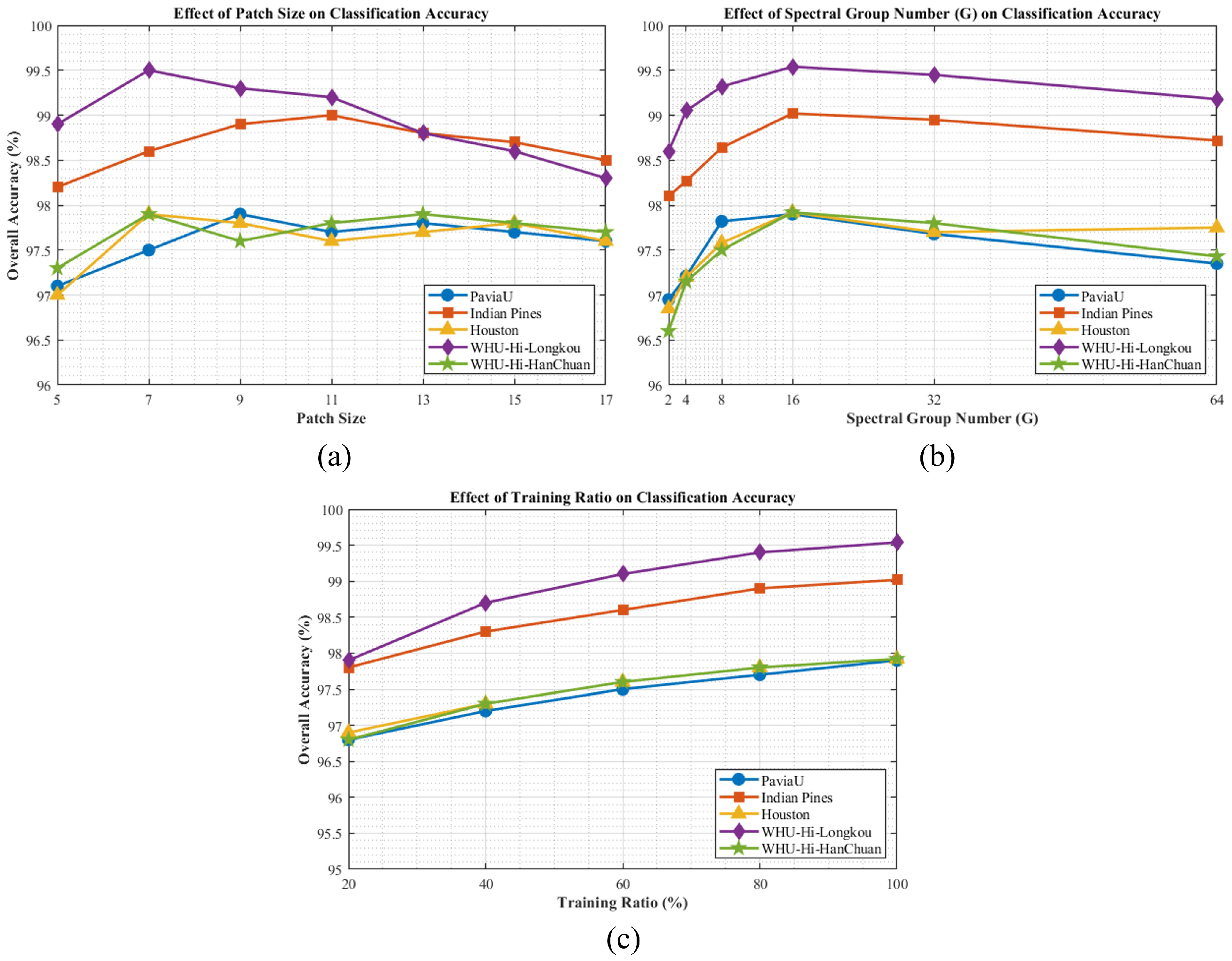
To assess the robustness and adaptability of BiMambaHSI, we further investigated the influence of three key factors: patch size, spectral group number (G) in the SSMB module, and training ratio. The experimental results are summarized in Figure 13. Patch size determines the extent of local spatial context. As shown in Figure 13a, accuracy increases with patch size until performance saturates or slightly declines after reaching a moderate scale. Small patches lack contextual semantics, while overly large patches introduce background noise and boundary smoothing. Most datasets achieved optimal performance with 9 × 9 or 11 × 11 patches, reflecting a balance between fine detail and context. G controls spectral partition granularity. Figure 13b shows that G = 16 consistently yields the highest accuracy across all datasets. Small G values merge a wide spectral range into one group, weakening local wavelength discrimination, while very large G values fragment continuous spectra, reducing global coherence. The stability of G = 16 across datasets supports the effectiveness of the proposed spectral grouping strategy. We further examined performance at 20%, 40%, 60%, 80%, and 100% labeled samples, as shown in Figure 13c. BiMambaHSI maintained an upward trend as supervision increases and achieves over 96% OA on PaviaU and Houston even with only 20% training samples, demonstrating good data efficiency. The small difference between 80% and 100% indicates early saturation of representation capacity.

4.3. Model Interpretation and Mechanism Analysis

To provide deeper insight into the design rationale and internal mechanisms of the proposed BiMambaHSI, we presented a concise interpretative analysis of its core modules—JGM and SSMB—and their collaborative effects.

(1) Forward–Backward Dependency Modeling. The JGM encoder was designed to enhance global spectral—spatial representation by incorporating both forward and backward state propagation. The forward propagation sequentially modeled dependencies along the scanning direction, while the backward propagation captured complementary contextual relations from the opposite direction. Their fusion enabled the model to perceive each pixel’s surrounding context in both preceding and succeeding orders, effectively mitigating direction-dependent bias in feature representation. Since both paths shared parameters within the Mamba formulation, this bidirectional extension introduced no additional theoretical complexity beyond the linear SSM framework.

(2) Spectral—Spatial Complementarity. While JGM emphasizes global spectral—spatial dependency modeling, the SSMB focused on local structural refinement. The spectral branch captured wavelength continuity and material-specific variations, whereas the spatial branch strengthened neighborhood coherence and boundary integrity. By combining both through adaptive fusion, the model achieved balanced representation learning—enhancing local discrimination without sacrificing global consistency. This design reflected the physical characteristics of hyperspectral imagery, where spatial adjacency and spectral smoothness jointly determined land-cover semantics.

4.4. Limitations and Future Work

BiMambaHSI still has certain limitations. First, although bidirectional modeling alleviates the shortcomings of unidirectionality, the fixed spectral grouping strategy may constrain its adaptability under varying spectral resolutions or sensor conditions. Second, this study relies on PCA for dimensionality reduction, but the optimal balance between information preservation and computational feasibility has not yet been explored further.

Future research could investigate adaptive spectral grouping strategies and multi-level bidirectional modeling structures to further enhance the model’s generalization ability. Beyond architectural refinements, it would also be valuable to examine alternative dimensionality reduction techniques or learned embeddings that strike a better balance between efficiency and information retention. In addition, extending BiMambaHSI to more challenging scenarios such as semi-supervised learning, cross-domain adaptation, and real-time applications may further improve its robustness, scalability, and practical utility in real-world hyperspectral tasks.

5. Conclusions

In this paper, we presented BiMambaHSI, a bidirectional state–space framework for hyperspectral image classification. BiMambaHSI introduces explicit bidirectional spectral—spatial state modeling and adaptive feature fusion while retaining pure SSM linear complexity. The framework integrates two complementary components: a joint spectral—spatial bidirectional gated Mamba (JGM) encoder that serializes hyperspectral cubes and models forward–backward dependencies, and a spatial—spectral mamba block (SSMB) that refines local spatial structures and spectral continuity through dual paths with learnable fusion. Experiments on five datasets demonstrate that BiMambaHSI achieves competitive performance across diverse spectral—spatial conditions. The results indicate that explicit bidirectional propagation and adaptive dual-path fusion provide a complementary modeling capability to existing methods, while preserving lightweight complexity characteristic of state–space models. These findings suggest that bidirectional spectral—spatial modeling is a promising direction for efficient and discriminative hyperspectral image classification.

References

1. Zhao, B.; Zhang, M.; Li, W.; Song, X.; Gao, Y.; Zhang, Y.; Wang, J. Intermediate domain prototype contrastive adaptation for spartina alterniflora segmentation using multitemporal remote sensing images. IEEE Trans. Geosci. Remote Sens. 2024, 62, 5401314. [Google Scholar] [CrossRef]
2. Zhao, B.; Zhang, M.; Wang, J.; Song, X.; Gui, Y.; Zhang, Y.; Li, W. Multiple attention network for spartina alterniflora segmentation using multitemporal remote sensing images. IEEE Trans. Geosci. Remote Sens. 2023, 61, 5402915. [Google Scholar] [CrossRef]
3. Sun, Z.; Liu, H.; Chen, N.; Yang, H.; Li, J.; Liu, C.; Pei, X. Spectral Channel Mixing Transformer with Spectral-Center Attention for Hyperspectral Image Classification. Remote Sens. 2025, 17, 3100. [Google Scholar] [CrossRef]
4. Yang, Z.; Li, H.; Wei, F.; Ma, J.; Zhang, T. WSC-Net: A Wavelet-Enhanced Swin Transformer with Cross-Domain Attention for Hyperspectral Image Classification. Remote Sens. 2025, 17, 3216. [Google Scholar] [CrossRef]
5. Mei, Y.; Fan, J.; Fan, X.; Li, Q. CSTC: Visual Transformer Network with Multimodal Dual Fusion for Hyperspectral and LiDAR Image Classification. Remote Sens. 2025, 17, 3158. [Google Scholar] [CrossRef]
6. Fu, D.; Zeng, Y.; Zhao, J. DFAST: A Differential-Frequency Attention-Based Band Selection Transformer for Hyperspectral Image Classification. Remote Sens. 2025, 17, 2488. [Google Scholar] [CrossRef]
7. Han, R.; Cheng, S.; Li, S.; Liu, T. Prompt-Gated Transformer with Spatial–Spectral Enhancement for Hyperspectral Image Classification. Remote Sens. 2025, 17, 2705. [Google Scholar] [CrossRef]
8. Zhao, B.; Li, Z.; Jiang, X.; Zhang, M.; Li, W.; Zhang, Y.; Song, X. Contrastive Adaptive Segmentation Method for Spartina Alterniflora Based on Intermediate Domain Prototypes. In Proceedings of the 2024 7th International Conference on Image and Graphics Processing, Beijing, China, 19–21 January 2024; pp. 85–91. [Google Scholar]
9. Wang, X.; Fan, Y. Multiscale densely connected attention network for hyperspectral image classification. IEEE J. Sel. Top. Appl. Earth Obs. Remote Sens. 2022, 15, 1617–1628. [Google Scholar] [CrossRef]
10. Cui, Y.; Xia, J.; Wang, Z.; Gao, S.; Wang, L. Lightweight spectral–spatial attention network for hyperspectral image classification. IEEE Trans. Geosci. Remote Sens. 2021, 60, 5510114. [Google Scholar] [CrossRef]
11. Ma, X.; Kang, X.; Qin, H.; Wang, W.; Ren, G.; Wang, J.; Liu, B. A Lightweight Hybrid Convolutional Neural Network for Hyperspectral Image Classification. IEEE Trans. Geosci. Remote Sens. 2023, 61, 5513714. [Google Scholar] [CrossRef]
12. Wang, D.; Hu, M.; Jin, Y.; Miao, Y.; Yang, J.; Xu, Y.; Qin, X.; Ma, J.; Sun, L.; Li, C.; et al. Hypersigma: Hyperspectral intelligence comprehension foundation model. IEEE Trans. Pattern Anal. Mach. Intell. 2025, 47, 6427–6444. [Google Scholar] [CrossRef]
13. Hong, D.; Han, Z.; Yao, J.; Gao, L.; Zhang, B.; Plaza, A.; Chanussot, J. SpectralFormer: Rethinking hyperspectral image classification with transformers. IEEE Trans. Geosci. Remote Sens. 2021, 60, 5518615. [Google Scholar] [CrossRef]
14. Zhao, Z.; Xu, X.; Li, S.; Plaza, A. Hyperspectral image classification using groupwise separable convolutional vision transformer network. IEEE Trans. Geosci. Remote Sens. 2024, 62, 5511817. [Google Scholar] [CrossRef]
15. Gu, A. Modeling Sequences with Structured State Spaces; Stanford University: Stanford, CA, USA, 2023. [Google Scholar]
16. Gu, A.; Goel, K.; Ré, C. Efficiently modeling long sequences with structured state spaces. arXiv 2021, arXiv:2111.00396. [Google Scholar]
17. Gu, A.; Johnson, I.; Goel, K.; Saab, K.; Dao, T.; Rudra, A.; Ré, C. Combining recurrent, convolutional, and continuous-time models with linear state space layers. Adv. Neural Inf. Process. Syst. 2021, 34, 572–585. [Google Scholar]
18. Liu, Y.; Tian, Y.; Zhao, Y.; Yu, H.; Xie, L.; Wang, Y.; Ye, Q.; Jiao, J.; Liu, Y. Vmamba: Visual state space model. Adv. Neural Inf. Process. Syst. 2024, 37, 103031–103063. [Google Scholar]
19. Dao, T.; Gu, A. Transformers are ssms: Generalized models and efficient algorithms through structured state space duality. arXiv 2024, arXiv:2405.21060. [Google Scholar] [CrossRef]
20. Li, Y.; Luo, Y.; Zhang, L.; Wang, Z.; Du, B. MambaHSI: Spatial–Spectral Mamba for Hyperspectral Image Classification. IEEE Trans. Geosci. Remote Sens. 2024, 62, 5524216. [Google Scholar] [CrossRef]
21. Cui, H.; Hayama, T. Hgmamba: Enhancing 3d human pose estimation with a hypergcn-mamba network. arXiv 2025, arXiv:2504.06638. [Google Scholar]
22. He, Y.; Tu, B.; Jiang, P.; Liu, B.; Li, J.; Plaza, A. IGroupSS-Mamba: Interval group spatial-spectral mamba for hyperspectral image classification. IEEE Trans. Geosci. Remote Sens. 2024, 62, 5538817. [Google Scholar] [CrossRef]
23. Zhao, B.; Zhang, M.; Li, W.; Gao, Y.; Wang, J. Domain Information Mining and State-Guided Adaptation Network for Multispectral Image Segmentation. IEEE Trans. Neural Netw. Learn. Syst. 2025, 36, 19849–19863. [Google Scholar] [CrossRef]
24. Zhang, J.; Sun, M.; Chang, S. Spatial and Spectral Structure-Aware Mamba Network for Hyperspectral Image Classification. Remote Sens. 2025, 17, 2489. [Google Scholar] [CrossRef]
25. Derosa, G.; Sahebkar, A.; Maffioli, P. The role of various peroxisome proliferator-activated receptors and their ligands in clinical practice. J. Cell. Physiol. 2018, 233, 153–161. [Google Scholar] [CrossRef]
26. Debes, C.; Merentitis, A.; Heremans, R.; Hahn, J.; Frangiadakis, N.; Van Kasteren, T.; Liao, W.; Bellens, R.; Pižurica, A.; Gautama, S.; et al. Hyperspectral and LiDAR data fusion: Outcome of the 2013 GRSS data fusion contest. IEEE J. Sel. Top. Appl. Earth Obs. Remote Sens. 2014, 7, 2405–2418. [Google Scholar] [CrossRef]
27. Baumgardner, M.F.; Biehl, L.L.; Landgrebe, D.A. 220 band aviris hyperspectral image data set: June 12, 1992 indian pine test site 3. Purdue Univ. Res. Repos. 2015, 10, R7RX991C. [Google Scholar]
28. Zhong, Y.; Hu, X.; Luo, C.; Wang, X.; Zhao, J.; Zhang, L. WHU-Hi: UAV-borne hyperspectral with high spatial resolution (H2) benchmark datasets and classifier for precise crop identification based on deep convolutional neural network with CRF. Remote Sens. Environ. 2020, 250, 112012. [Google Scholar] [CrossRef]
29. Zhong, Y.; Wang, X.; Xu, Y.; Wang, S.; Jia, T.; Hu, X.; Zhao, J.; Wei, L.; Zhang, L. Mini-UAV-borne hyperspectral remote sensing: From observation and processing to applications. IEEE Geosci. Remote Sens. Mag. 2018, 6, 46–62. [Google Scholar] [CrossRef]
30. Roy, S.K.; Jamali, A.; Chanussot, J.; Ghamisi, P.; Ghaderpour, E.; Shahabi, H. SimPoolFormer: A two-stream vision transformer for hyperspectral image classification. Remote Sens. Appl. Soc. Environ. 2025, 37, 101478. [Google Scholar] [CrossRef]
31. Sun, L.; Zhao, G.; Zheng, Y.; Wu, Z. Spectral–Spatial Feature Tokenization Transformer for Hyperspectral Image Classification. IEEE Trans. Geosci. Remote Sens. 2022, 60, 5522214. [Google Scholar] [CrossRef]
Figure 1. The original image and labeled ground truth of Pavia University dataset.
Remotesensing 17 03676 g001
Figure 2. The original image and labeled ground truth of Houston dataset.
Remotesensing 17 03676 g002
Figure 3. The original image and labeled ground truth of Indian Pines dataset.
Remotesensing 17 03676 g003
Figure 4. The original image and labeled ground truth of WHU-Hi-HanChuan dataset.
Remotesensing 17 03676 g004
Figure 5. The original image and labeled ground truth of WHU-Hi-LongKou dataset.
Remotesensing 17 03676 g005
Figure 6. Overview of the BiMambaHSI framework.
Remotesensing 17 03676 g006
Figure 7. Overview of the spatial—spectral Mamba block (SSMB).
Remotesensing 17 03676 g007
Figure 8. The classification maps of all methods in the Pavia University dataset: (a) image, (b) ground Truth, (c) GSCNet, (d) HyperSIGMA, (e) Lite-HCNNet, (f) MSDAN, (g) SimpoolFormer, (h) SpectralFormer, (i) SSFTT, (j) MambaHSI, (k) HGMamba, and (l) BiMambaHSI.
Remotesensing 17 03676 g008
Figure 9. The classification maps of all methods in the Houston dataset: (a) image, (b) ground truth, (c) GSCNet, (d) HyperSIGMA, (e) Lite-HCNNet, (f) MSDAN, (g) SimpoolFormer, (h) SpectralFormer, (i) SSFTT, (j) MambaHSI, (k) HGMamba, and (l) BiMambaHSI.
Remotesensing 17 03676 g009
Figure 10. The classification maps of all methods in the Indian Pines dataset: (a) image, (b) ground truth, (c) GSCNet, (d) HyperSIGMA, (e) Lite-HCNNet, (f) MSDAN, (g) SimpoolFormer, (h) SpectralFormer, (i) SSFTT, (j) MambaHSI, (k) HGMamba, and (l) BiMambaHSI.
Remotesensing 17 03676 g010
Figure 11. The classification maps of all methods in the WHU-Hi-HanChuan dataset: (a) image, (b) ground truth, (c) GSCNet, (d) HyperSIGMA, (e) Lite-HCNNet, (f) MSDAN, (g) SimpoolFormer, (h) SpectralFormer, (i) SSFTT, (j) MambaHSI, (k) HGMamba, and (l) BiMambaHSI.
Remotesensing 17 03676 g011
Figure 12. The classification maps of all methods in the WHU-Hi-LongKou dataset: (a) image, (b) ground truth, (c) GSCNet, (d) HyperSIGMA, (e) Lite-HCNNet, (f) MSDAN, (g) SimpoolFormer, (h) SpectralFormer, (i) SSFTT, (j) MambaHSI, (k) HGMamba, and (l) BiMambaHSI.
Remotesensing 17 03676 g012
Figure 13. Parameter sensitivity analysis of BiMambaHSI across five datasets: (a) patch size, (b) spectral group number (G), and (c) training sample ratio.
Remotesensing 17 03676 g013