Dehazing of Panchromatic Remote Sensing Images Based on Histogram Features

Highlights

What are the main findings?

• A correlation exists between the histogram features of panchromatic remote sensing images and the transmission. The relation equation between the average occurrence differences between the adjacent gray levels (AODAG) feature of the plain image patch and the transmission, and the relation equation between the average distance to the gray-level gravity center (ADGG) feature of the mixed image patch and the transmission are established, respectively.
• The atmospheric light of different regions in the remote sensing image may be different. The threshold segmentation method is applied to calculate the atmospheric light of each image patch based on the maximum gray level of the patch separately.

What is the implication of the main finding?

• The transmission map is obtained according to the statistical relation equation without relying on the color information, which is beneficial for the dehazing of panchromatic remote sensing images.
• A refined atmospheric light map is obtained, resulting in a more uniform brightness distribution in the dehazed image.

Abstract

During long-range imaging, the turbid medium in the atmosphere absorbs and scatters light, resulting in reduced contrast, a narrowed dynamic range, and obscure detail information in remote sensing images. The prior-based method has the advantages of good real-time performance and a wide application range. However, few of the existing prior-based methods are applicable to the dehazing of panchromatic images. In this paper, we innovatively propose a prior-based dehazing method for panchromatic remote sensing images through statistical histogram features. First, the hazy image is divided into plain image patches and mixed image patches according to the histogram features. Then, the features of the average occurrence differences between adjacent gray levels (AODAGs) of plain image patches and the features of the average distance to the gray-level gravity center (ADGG) of mixed image patches are, respectively, calculated. Then, the transmission map is obtained according to the statistical relation equation. Then, the atmospheric light of each image patch is calculated separately based on the maximum gray level of the image patch using the threshold segmentation method. Finally, the dehazed image is obtained based on the physical model. Extensive experiments in synthetic and real-world panchromatic hazy remote sensing images show that the proposed algorithm outperforms state-of-the-art dehazing methods in both efficiency and dehazing effect.

1. Introduction

As an important product of Earth observation technology, remote sensing images (RSIs) play an increasingly important role in people’s production and life. In particular, panchromatic remote sensing images have the advantages of a high spatial resolution and a high signal-to-noise ratio (SNR) [1]. However, in the process of long-range imaging, the turbid medium in the atmosphere absorbs and scatters light, resulting in reduced contrast, a narrowed dynamic range, and obscure detail information in remote sensing images. The poor visual effect of the hazy images directly limits many image understanding and computer vision applications such as target tracking, intelligent navigation, image classification, visual monitoring, and remote sensing [2]. The dehazing technique plays an important role in the Earth observation system by restoring hazy images and improving the quality of remote sensing images.

After decades of development, image dehazing methods have achieved significant improvements in performance and efficiency. Image dehazing methods are mainly categorized into prior-based dehazing algorithms, learning-based dehazing algorithms [3], and histogram-based dehazing algorithms. The prior-based dehazing algorithms realize the estimation of unknown parameters in the physical model by mining the prior knowledge of hazy or clear images to achieve image restoration. He [4] statistically derived the dark channel prior (DCP), which holds that most non-sky patches in haze-free outdoor images contain some pixels which have very low intensities in at least one color channel. Atmospheric Illumination Prior [5], Super-Pixel Scene Prior [6], and Gray Haze-Line Prior [7] found that haze only affects a specific component of the color space such as YC_rC_b, Lab, and YUV, and has little effect on other components. Saturation Line Prior [8] and Color Attenuation Prior [9] derived the transmission by statistically calculating the color information of clear or hazy images. Low-Rank and Sparse Prior [10] and Rank-One Prior [11] realized dehazing by computing the features of the transformed image. Haze Smoothness Prior [12] regarded the hazy image as the sum of the clear image and corresponding haze layer, and realized dehazing based on the fact that the haze layer is smoother than the clear image. Tan et al. [13] proposed Mixed Atmosphere Prior, which divided the hazy image into foreground and background areas, and accurately calculated the atmospheric light maps of the foreground and background areas, respectively. Most of the prior-based dehazing approaches need to rely on the color information of the image, which will be ineffective for panchromatic images without color information. Therefore, it is of great importance to mine the prior knowledge of panchromatic hazy or clear images to achieve dehazing.

Learning-based dehazing algorithms have received extensive attention from scholars in the last decade. Cai et al. proposed an end-to-end network, DehazeNet [14], which employs a convolutional neural network (CNN) to realize the estimation of transmission. Subsequently, many CNN-based image dehazing methods were proposed [15,16,17,18]. Yeh et al. [19] decomposed the hazy image into a base component and a detail component, and utilized a multi-scale deep residual and U-Net to learn the base component of hazy and clear images. The clear image is obtained by integrating the dehazed base component and the enhanced detail component. The attention mechanism-based generative adversarial network (GAN) for the cloud removal algorithm was introduced for satellite images [20]. Xu et al. [21] developed a multi scale GAN that removes thin clouds from cloudy scenes. Sun et al. [22] introduced UME-Net, an unsupervised multi-branch network designed to restore the high-frequency details often lost in hazy images. The improved GAN achieves image dehazing by training unpaired real-world hazy and clean images [23,24]. In order to improve the computational efficiency, a lightweight dehaze network (LDN) [25,26,27] has been proposed to reduce the computational complexity while achieving satisfactory dehazing results. Benefiting from the global modeling capability and long-term dependency features, the Transformer and its improved architectures [28,29,30,31,32,33] have achieved promising results in the field of remote sensing image dehazing. Ding et al. [34] used conditional variational autoencoders (CVAEs) to generate multiple restoration images, and then fused them through a dynamic fusion network (DFN) to obtain the final dehazing images. Ma et al. [35] proposed an encoder–decoder structure combined with a mixture attention block for haze removal in nighttime light remote sensing images. The integration of a prior-based and a learning-based dehazing method also achieved pleasing results [36,37]. Learning-based dehazing algorithms rely heavily on training data and sometimes fail for remote sensing images, especially aerial remote sensing images. Moreover, the computational complexity of learning-based dehazing methods is too high, and they are not easy to implement on low-power embedded systems. Zhang et al. [38] proposed a dual-task collaborative mutual promotion framework that integrates depth estimation and dehazing through an interactive mechanism.

The histogram of an image can reflect the distribution of gray levels. Its horizontal axis represents the gray level, and the vertical axis represents the number of occurrences of the corresponding gray level. The histogram can also reflect the dynamic range of the image. The greater the concentration of the haze, the more concentrated the distribution of gray levels, and the smaller the dynamic range of the image. On the contrary, the smaller the concentration of the haze, the more dispersed the distribution of gray levels, and the larger the dynamic range of the image. Assuming that the image $I=\left\{I(i,j)\right\}$ consists of $L$ discrete gray levels, denoted as $\left\{K_0,K_1,\cdots ,K_{L-1}\right\}$, $I(i,j)$ denotes the gray value of pixel $(i,j)$, and $I(i,j)\in \left\{K_0,K_1,\cdots ,K_{L-1}\right\}$. The histogram equalization (HE) algorithm achieves the objectives of expanding dynamic range and enhancing contrast by shaping the probability density function (PDF) of gray levels to approximate a uniform distribution [39]. It can be applied to image dehazing. The brightness-preserving bi-histogram equalization (BBHE) addresses the issue of uneven brightness in local regions of dehazed images [40]. Two-dimensional histogram algorithms [41,42] effectively preserve local detail information and brightness while enhancing contrast. The logarithmic mapping-based histogram equalization (LMHE) [43] makes dehazed images more consistent with human visual perception. Adaptive histogram equalization [44,45] achieves high image quality in dehazed images by seeking optimal adjustment parameters. Reflectance-guided histogram equalization [46] enhances both global and local contrast while addressing the uneven illumination issue. The aforementioned histogram equalization methods do not use an atmosphere scattering model and are categorized as image enhancement techniques. They achieve haze removal by directly transforming the histogram. Our algorithm innovatively establishes a relation equation between histogram features and transmission, then employs an atmosphere scattering model to perform haze removal. Our approach belongs to the category of image restoration methods, yielding more natural dehazed images that closely resemble clear images.

There are also some fusion-based dehazing methods that have achieved satisfactory results. Guo et al. [47] fused the transmission obtained by DCP and the transmission calculated based on the constraints to generate the final transmission. Hong et al. [48] divided the hazy image into patches, and then set a series of low-to-high transmissions manually for each patch. The physical dehazing model is used to restore each patch, and the patch with the best dehazing effect is selected for fusion. The dehazing effect of fusion-based methods is easily affected by the selection of parameters, and inappropriate parameter settings will reduce the dehazing effect. Variation-based or optimization methods have also been widely used in image dehazing. By integrating structure-aware models, the variation-based dehazing methods achieve transmission estimation and refinement [49]. Ding et al. [50] used a variation method to obtain fine depth information of the scene, and then computed the transmission using a physical model. Meng et al. [51] incorporated a constraint into an optimization model to estimate the unknown scene transmission. Liu et al. [52] introduced a novel variational framework for nighttime image dehazing that leverages hybrid regularization to enhance visibility and structural clarity in hazy scenes. Although many optimization methods for variational problems were proposed [53,54], the variation-based dehazing algorithms easily fall into the local optimal solution, and sometimes can not achieve a satisfactory dehazing effect. Image enhancement methods can increase the contrast of the image and highlight the detail information, which is suitable for the dehazing of panchromatic images. Jang et al. realized the dehazing of optical remote sensing images by using a hybrid intensity transfer function based on Retinex theory [55]. Khan et al. achieved dehazing by enhancing the detail information of hazy images through wavelet transforms [56]. The image-enhancement-based dehazing methods sometimes lead to the phenomenon of the oversaturation of intensity, resulting in the loss of detailed information in the dehazed image.

The light reflected from the ground scene and the atmospheric light enter into the sensor through a complex process in hazy conditions. The degradation process of remote sensing images is shown in Figure 1.

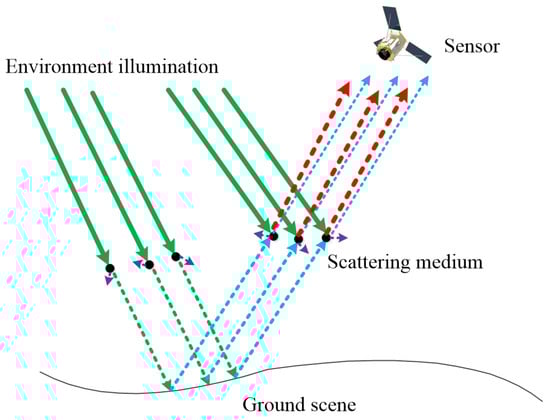
Figure 1. Diagram of the degradation process of remote sensing images.

The atmosphere scattering model [57,58] is the most classical physical model to describe the degradation of hazy images, which is abstracted as follows:

$$I(x)=J(x)t(x)+A(1-t(x))$$

(1)

where $x$ is the pixel coordinate in the image, $I(x)$ represents the hazy image, $J(x)$ represents the clear image. $t(x)$ denotes the transmission, which is usually considered to be constant in the local image patch. $A$ represents the atmospheric light. The transmission can be expressed as $t(x)=\exp [-{\beta }_{sc}d(x)]$, where ${\beta }_{sc}$ represents the atmospheric scattering coefficient and $d(x)$ represents the imaging distance. It can be observed that as the imaging distance increases, the transmission decreases. In the atmosphere scattering model, the term $J(x)t(x)$ represents the portion of light reflected from the scene that reaches the sensor after attenuation through the turbid medium, while the term $A(1-t(x))$ represents the portion of atmospheric light scattered directly into the sensor. Image dehazing based on the atmosphere scattering model is performed to estimate $t(x)$ and $A$, and then obtains the clear image $J(x)$.

The histogram characteristics can directly reflect the degree to which a remote sensing image is affected by haze. Moreover, histogram characteristics are universal, existing in both color and panchromatic images. Aiming at the problem that most of the existing prior-based dehazing methods are not applicable to panchromatic images without color information, we innovatively propose a dehazing algorithm based on histogram features (HFs) for panchromatic remote sensing images. The HF algorithm runs efficiently and can be executed without relying on high-performance hardware platforms such as GPUs. The innovative contributions can be summarized as follows.

(1)

Without relying on the color information of the image, dehazing is achieved by extracting histogram features of the panchromatic remote sensing image. According to the histogram features, the hazy image is divided into plain image patches and mixed image patches, and the dehazing is carried out, respectively.

(2)

The relation equation between the AODAG feature of the plain image patch and the transmission, and the relation equation between the ADGG feature of the mixed image patch and the transmission are established, respectively. Eight-neighborhood mean filtering and Gaussian filtering are applied to smooth the original transmission map.

(3)

According to the characteristics of atmospheric light distribution in remote sensing images, the threshold segmentation method is applied to calculate the atmospheric light of each image patch based on the maximum gray level of the patch separately, which makes the intensity of the dehazed images more uniform.

The article is organized as follows. Section 2 describes the key details of the proposed HF algorithm. The results of panchromatic remote sensing image dehazing experiments are given in Section 3. The proposed algorithm is discussed in Section 4. Finally, a conclusion is presented in Section 5.

2. Materials and Methods

The proposed HF algorithm is presented at a detailed level, and the schematic diagram is depicted in Figure 2. First, the hazy image is divided into plain image patches and mixed image patches according to the histogram features. Then, the AODAG features of plain patches and the ADGG features of mixed patches are computed, respectively, and the initial transmission map is calculated according to the statistical relational equation. Then, the eight-neighborhood mean filtering and the Gaussian filtering are carried out to obtain the final transmission map. Then, the threshold segmentation method is applied to calculate the atmospheric light of each patch based on the maximum gray level of the image patch, and Gaussian filtering is applied to obtain the final atmospheric light map. Finally, the dehazed image is obtained based on the atmosphere scattering model.

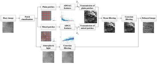
Figure 2. Schematic of the proposed dehazing method based on histogram features.

2.1. Histogram Features

We utilize histogram features to divide the hazy image into plain patches and mixed patches and compute the transmission map. The detailed calculation steps are shown below.

2.1.1. Patch Classification

Inspired by [48], we divide the hazy image into image patches of size $N_p\times N_p$. The number of pixels contained in an image patch is $N_s=N_p\times N_p$, and $N_p$ is defined as 15. In this paper, the transmission is considered to be constant within a certain image patch. Based on the characteristics of the histogram, the image patches are divided into plain image patches and mixed image patches. The image patches with a relatively concentrated gray-level distribution are defined as plain image patches, and the image patches with a relatively dispersed gray-level distribution are defined as mixed image patches, as shown in Figure 3. We divide plain image patches and mixed image patches according to the following rules. Assume that $I_m$ is the gray level with the highest number of occurrences in each image patch. The gray-level neighborhood ${\mathsf{\Omega }}_m$ is determined with $I_m$ as the center and $R_m$ as the radius, and the value of $R_m$ is set to 3. The sum of occurrences of all gray levels in neighborhood ${\mathsf{\Omega }}_m$ is calculated with the following equation:

$$N_m={\displaystyle \sum _{I_i\in {\mathsf{\Omega }}_m}{n}_i},$$

(2)

where $n_i$ represents the number of occurrences of gray level $I_i$. When $N_m/N_s$ is larger than the threshold value $T_m$, the image patch is defined as the plain image patch. Otherwise, the image patch is defined as the mixed image patch. The value of $T_m$ is set to 0.65. The classification formula of patches is defined as follows:

$$P=\left\{\begin{array}{l}{P}_p,{\displaystyle \frac{N_m}{N_s}}>T_m;\\ P_m,else\end{array}\right.,$$

(3)

where $P_p$ represents the plain image patch, and $P_m$ represents the mixed image patch.

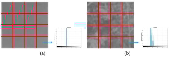
Figure 3. Diagram of the classification of patches. (a) Plain patches. (b) Mixed patches.

2.1.2. Plain Patch Feature

In the plain image patch of the hazy image, the distribution of gray levels is relatively concentrated, and the histogram of the plain image patch is shown in Figure 4. It can be seen that on the left and right sides of the gray level with the highest number of occurrences, the number of occurrences of the gray level approximates the characteristic of decreasing sequentially. We obtain the prior for plain image patches as follows. The lower the transmission of the plain image patch, the larger the average occurrence differences between adjacent gray levels, i.e., the steeper the gray levels appear in the histogram.

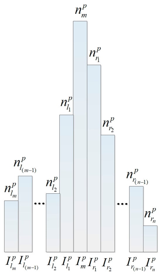
Figure 4. Histogram of the plain image patch.

The AODAG feature of the plain image patch is calculated as follows. Assume that $I_m^p$ is the gray level with the highest number of occurrences in the plain patch, and the number of occurrences of $I_m^p$ is $n_m^p$. The gray levels on the right side of $I_m^p$ are sequentially denoted as $I_{r_1}^p$, $I_{r_2}^p$, …, $I_{r_{(n-1)}}^p$, $I_{r_n}^p$, and their corresponding numbers of occurrences are denoted as $n_{r_1}^p$, $n_{r_2}^p$, …, $n_{r_{(n-1)}}^p$, $n_{r_n}^p$, respectively. The numbers of occurrences of all the gray levels on the right side of $I_{r_n}^p$ are zero. The average occurrence differences between adjacent gray levels on the right side of $I_m^p$ can be expressed as follows:

$$d_r={\displaystyle \frac{(n_m^p-n_{r_1}^p)+(n_{r_1}^p-n_{r_2}^p)+\cdot \cdot \cdot +(n_{r_{(n-1)}}^p-n_{r_n}^p)+(n_{r_n}^p-0)}{n+1}}.$$

(4)

We eliminate the middle terms of the numerator and the simplified formula can be expressed with the following equation:

$$d_r={\displaystyle \frac{n_m^p}{n+1}}.$$

(5)

Considering the stability of the proposed algorithm, we replace $n_m^p$ with the mean of the top three gray-level occurrences. $d_r$ can be denoted as follows:

$$d_r={\displaystyle \frac{{\displaystyle \sum _{i=1}^3{n}_{m_i}^p}}{3(n+1)}},$$

(6)

where $n_{m_1}^p$, $n_{m_2}^p$, $n_{m_3}^p$ are the top three gray-level occurrences, respectively. Assume that the gray levels on the left side of $I_m^p$ are sequentially denoted as $I_{l_1}^p$, $I_{l_2}^p$, ⋯, $I_{l_{(m-1)}}^p$, $I_{l_m}^p$, and their corresponding numbers of occurrences are denoted as $n_{l_1}^p$, $n_{l_2}^p$, ⋯, $n_{l_{(m-1)}}^p$, $n_{l_m}^p$, respectively. The numbers of occurrences of all the gray levels on the left side of $I_{l_m}^p$ are zero. Similarly, the average occurrence differences between adjacent gray levels on the left side of $I_m^p$ can be expressed as follows:

$$d_l={\displaystyle \frac{n_m^p}{m+1}}.$$

(7)

We replace $n_m^p$ with the mean of the top three gray-level occurrences. $d_l$ can be denoted as follows:

$$d_l={\displaystyle \frac{{\displaystyle \sum _{i=1}^3{n}_{m_i}^p}}{3(m+1)}},$$

(8)

The general AODAG feature can be obtained by calculating the arithmetic mean of $d_r$ and $d_l$, as expressed by the following formula:

$$d_g={\displaystyle \frac{d_r+d_l}{2}}.$$

(9)

2.1.3. Mixed Patch Feature

Due to haze interference, gray levels will be clustered together to form one or two peaks in the histogram of the mixed image patch, as shown in Figure 5. From the histogram, it can be seen that the number of occurrences of the gray levels on the left and right sides of the peak approximates the characteristic of decreasing sequentially. The main-peak gray level $I_m^m$ is defined as the gray level with the highest number of occurrences in the histogram. If a secondary-peak gray level $I_s^m$ exists, it must satisfy the following conditions: (1) It is generated among the top $T_{sr}$ gray levels by occurrence frequency, while being the highest-ranked gray level that satisfies both condition (2) and condition (3). The value of $T_{sr}$ is set to 6. (2) The number of its occurrences is greater than the threshold value $T_{sn}$, which is set to 15 in this paper. (3) The distance between it and the main-peak gray level is greater than the threshold value $T_{sd}$, which is set to 18.

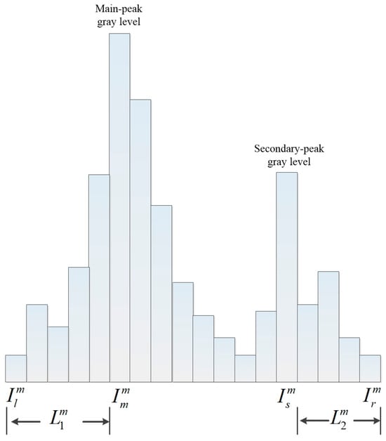
Figure 5. Histogram of the mixed image patch.

We define the gray level range in the histogram of the mixed image patch as $S=\left[I_l^m,I_r^m\right]$. The number of occurrences of all the gray levels on the left side of $I_l^m$ is zero and the number of occurrences of all the gray levels on the right side of $I_r^m$ is zero. If only the main-peak gray level exists in the histogram of the mixed image patch, define the main gray-level domain as $S$. If both the main-peak gray level and the secondary-peak gray level exist in the histogram of the mixed image patch, they may overlap. The main gray-level domain and the secondary gray-level domain are defined according to the following steps. First, the smaller and larger values between the main-peak gray level and the secondary-peak gray level can be calculated with the following equation:

$$\left\{\begin{array}{l}{I}_{\min }^m=\min (I_m^m,I_s^m)\\ I_{\max }^m=\max (I_m^m,I_s^m)\end{array}\right.,$$

(10)

where $I_{\min }^m$ represents the smaller value, $I_{\max }^m$ represents the larger value. Then, the distance $L_1^m$ from $I_l^m$ to $I_{\min }^m$ and the distance $L_2^m$ from $I_{\max }^m$ to $I_r^m$ can be computed as follows:

$$L_1^m=I_{\min }^m-I_l^m,$$

(11)

$$L_2^m=I_r^m-I_{\max }^m.$$

(12)

Since the left and right sides of the peak gray level present an approximate symmetrical shape, the range of the gray-level domain $S_1$ where $I_{\min }^m$ resides is determined to be $\left[I_l^m,I_l^m+2L_1^m\right]$ and the range of the gray-level domain $S_2$ where $I_{\max }^m$ resides is determined to be $\left[I_r^m-2L_2^m,I_r^m\right]$. If the main-peak gray level $I_m^m$ resides in the domain $S_1$, then $S_1$ is the main gray-level domain and $S_2$ is the secondary gray-level domain. Otherwise, $S_1$ is the secondary gray-level domain and $S_2$ is the main gray-level domain. We obtain the prior for mixed image patches as follows. The lower the transmission of the mixed image patch, the smaller the average distance to the gray-level gravity center in the gray-level domain. The feature of ADGG is calculated as follows.

The gravity center of the gray levels in the range of $[I_a,I_b]$ of the histogram is calculated with the following equation:

$$I_g=F(I_a,I_b)={\displaystyle \sum _{i=a}^b{n}_i{I}_i}/{\displaystyle \sum _{i=a}^b{n}_i},$$

(13)

where $n_i$ represents the number of occurrences of the gray level $I_i$, and not all $n_i$ are zero. The average distance to the gray-level gravity center for gray levels with a non-zero number of occurrences in the range of $[I_a,I_b]$ is calculated as follows:

$$d_e=D(I_a,I_b,I_g)={\displaystyle \sum _{k=a}^b\left|I_k-I_g\right|}/N_{nz},$$

(14)

where $I_k$ represents the gray level with non-zero occurrences in the range of $[I_a,I_b]$, $N_{nz}$ represents the number of gray levels with non-zero occurrences. When only the main-peak gray level exists in the histogram of the mixed image patch, the ADGG feature is calculated using Equations (13) and (14), where $I_a=I_l^m$ and $I_b=I_r^m$. When both the main-peak gray level and the secondary-peak gray level exist in the histogram of the mixed image patch, the ADGG feature in the gray-level domain $S_1$ is calculated as follows:

$$I_{g_1}=F(I_l^m,I_l^m+2L_1^m),$$

(15)

$$d_{e_1}=D(I_l^m,I_l^m+2L_1^m,I_{g_1}),$$

(16)

where $I_{g_1}$ is the gravity center of the gray levels in the gray-level domain $S_1$. The ADGG feature in the gray-level domain $S_2$ is calculated as follows:

$$I_{g_2}=F(I_r^m-2L_2^m,I_r^m),$$

(17)

$$d_{e_2}=D(I_r^m-2L_2^m,I_r^m,I_{g_2}),$$

(18)

where $I_{g_2}$ is the gravity center of the gray levels in the gray-level domain $S_2$. The general ADGG feature is computed with the following equation:

$$d_{e_g}={\omega }_1{d}_{e_1}+{\omega }_2{d}_{e_2},$$

(19)

where ${\omega }_1$ and ${\omega }_2$ represent the weight coefficients, and we consider that the gray levels within $S_1$ and $S_2$ are aggregated to the peak gray level to the same extent in this paper. Set both the values of ${\omega }_1$ and ${\omega }_2$ to 0.5.

2.2. Statistical Relation Equation

2.2.1. Hazy Image Synthesis

In order to obtain the relation equation between the histogram feature and the transmission of the hazy image patch, inspired by the method of synthesizing a hazy image in [59,60], we artificially synthesize the hazy panchromatic images using Equation (1). The atmospheric light $A$ is randomly selected in the range of $[0.7,1]$ and the transmission $t$ is randomly selected in the range of $[0.1,0.7]$. Clear panchromatic images have two sources: one is panchromatic remote sensing images captured by the Jilin-1 satellite, and the other is panchromatic remote sensing images synthesized from color images. Color remote sensing images are selected from the clear reference images in the RICE-1 dataset [61] and the RSHaze dataset [62], and the clear panchromatic images are synthesized based on the quantum efficiency response curve of the panchromatic sensors. The quantum efficiency response curve of a certain panchromatic sensor is shown in Figure 6, and the color image is synthesized into a panchromatic image according to the proportionality of the quantum efficiency values at the center wavelengths of the R channel, the G channel, and the B channel. The intensity of the panchromatic image is calculated as follows:

$$I_P(i,j)={\omega }_R\cdot I_R(i,j)+{\omega }_G\cdot I_G(i,j)+{\omega }_B\cdot I_B(i,j),$$

(20)

where $(i,j)$ is the pixel coordinate in the image, $I_R$, $I_G$, and $I_B$ represent the intensity of the R channel, the G channel, and the B channel, respectively, and ${\omega }_R$, ${\omega }_G$, and ${\omega }_B$ represent the weighting coefficients of the intensity of the R channel, the G channel, and the B channel, respectively.

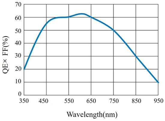
Figure 6. Diagram of the quantum efficiency response curve.

The synthesized hazy panchromatic image datasets are of three kinds according to their sources, which are denoted as JilinP-1, RICEP-1, and RSPHaze. The three datasets cover different types of scenarios, including mountains, deserts, wetlands, and cities. Each kind of image dataset contains 100 images with a resolution size of 512 × 512. The relation equation between the AODAG feature and the transmission for the plain image patch, and the relation equation between the ADGG feature and the transmission for the mixed image patch are established, respectively.

2.2.2. AODAG Relation Equation

Images of the same scene from JilinP-1, RICEP-1, and RSPHaze datasets are selected for AODAG feature statistics, and the relationship between AODAG features and transmission of 600 plain image patches in each dataset is shown in Figure 7.

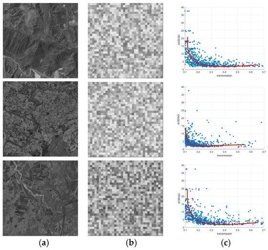
Figure 7. Plot of AODAG features versus transmission for plain image patches. (First row) Ji linP-1 dataset. (Second row) RICEP-1 dataset. (Third row) RSPHaze dataset. (a) Clear images. (b) Synthesized hazy images. (c) Relationship diagrams. The X-axis represents the transmission and the Y-axis represents AODAG features.

It can be seen that for images of the same scene in the same dataset, the relationship between AODAG features and the transmission for plain image patches approximately satisfies the hyperbolic relation equation, which is defined as follows:

$$y_p=t/k_p+k_p/t,$$

(21)

where $t$ denotes the transmission, $y_p$ denotes the AODAG feature, and $k_p$ denotes the parameter to be determined. For images of different scenes in different datasets, the shape of the hyperbola is slightly different due to different sensors and different textures of the scenes. There is only one pending parameter in Equation (21), and the smaller the value of $k_p$, the closer the vertex of the hyperbola is to the coordinate origin. Conversely, the larger the value of $k_p$, the further the vertex of the hyperbola is to the coordinate origin.

2.2.3. ADGG Relation Equation

Images of the same scene from JilinP-1, RICEP-1, and RSPHaze datasets are selected for ADGG feature statistics, and the relationship between ADGG features and the transmission of 900 mixed image patches in each dataset is shown in Figure 8.

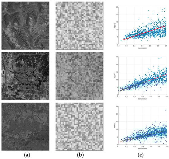
Figure 8. Plot of ADGG features versus transmission for mixed image patches. (First row) JilinP-1 dataset. (Second row) RICEP-1 dataset. (Third row) RSPHaze dataset. (a) Clear images. (b) Synthesized hazy images. (c) Relationship diagrams. The X-axis represents the transmission and the Y-axis represents ADGG features.

It can be seen that for images of the same scene in the same dataset, the relationship between ADGG features and transmission for mixed image patches approximately satisfies the linear relation equation. The straight line passes through the coordinate origin, and the linear relation equation is defined as follows:

$$y_m=k_m\cdot t,$$

(22)

where $t$ denotes the transmission, $y_m$ denotes the ADGG feature, and $k_m$ denotes the slope of the straight line. $k_m$ is the only parameter to be determined, and the values of $k_m$ are slightly different for images of different scenes in different datasets. It can be seen from relationship diagrams that the points are denser in the low value interval of transmission, and the points are gradually dispersed with the increase in transmission. This phenomenon indicates that the linear equation demonstrates good consistency in the low transmission interval.

2.2.4. Relation Equation Fitting

The least squares method [63] is employed to fit the relation equation between the histogram features of image patches and transmission. For AODAG features, the sum of squared errors (SSE) is expressed as follows:

$$SS{E}_p={\displaystyle \sum _{i=1}^N{(y_i-(x_i/k_p+k_p/x_i))}^2},$$

(23)

where $N$ represents the number of samples, $(x_i,y_i)$ represents the observed data point, $k_p$ represents the coefficient to be solved. For ADGG features, the SSE is expressed as follows:

$$SS{E}_m={\displaystyle \sum _{i=1}^N{(y_i-k_m\cdot x_i)}^2},$$

(24)

where $N$ represents the number of samples, $(x_i,y_i)$ represents the observed data point, $k_m$ represents the coefficient to be solved. The values of $k_p$ and $k_m$ are calculated through statistical analysis of a large number of image samples. For images of different scenes in different datasets, the values of $k_p$ and $k_m$ vary only within a narrow range. The variation range of $k_p$ is $[0.4,1.1]$, and the variation range of $k_m$ is $[16,23]$.

2.3. Atmospheric Light Calculation

In most of the dehazing methods, the whole image corresponds to the same atmospheric light [4,8,9,11]. However, due to the large coverage area of the remote sensing image and the long propagation path of the light reflected from the scene, the atmospheric light of different regions in the remote sensing image may be different [13]. Due to the maximum gray level in each image patch that has been obtained in the process of histogram feature calculation, we calculate the atmospheric light of each image patch separately. The segmentation threshold is defined as follows:

$$T_A={\displaystyle \frac{{\displaystyle \sum _{(x,y)\in X}I(x,y)}}{w\times h}},$$

(25)

where $I(x,y)$ represents the intensity of the image at the position $(x,y)$, $w$ and $h$ represent the width and height of the image, respectively. If the maximum gray level in the image patch is smaller than the threshold $T_A$, the atmospheric light corresponding to the image patch is set to $T_A$. Otherwise, the atmospheric light corresponding to the image patch is set to the maximum gray level in the image patch. The atmospheric light can be expressed as follows:

$$A_b(i)=\left\{\begin{array}{l}{T}_A,I_m(i)<T_A\\ I_m(i),else,\end{array}\right.$$

(26)

where $A_b(i)$ represents the atmospheric light corresponding to the image patch with index $i$, and $I_m(i)$ represents the maximum gray level in the image patch with index $i$. The atmospheric light $A_b(i)$ of all image patches together forms the atmospheric light map $A_w$ of the whole image.

After obtaining the atmospheric light map $A_w$ of the entire image, the atmospheric light map is smoothed by Gaussian filtering, and the filtered atmospheric light map is computed as follows:

$$A_g(x,y)=G_{{\sigma }_a}(A_w(x,y)),$$

(27)

where $(x,y)$ represents the position of the pixel in the image, $G_{{\sigma }_a}$ represents the Gaussian filtering function with standard deviation ${\sigma }_a$, and the value of ${\sigma }_a$ is set to 12.5. The Gaussian filter is defined with the following equation:

$$G_{{\sigma }_a}(x,y)={\displaystyle \frac{1}{2\pi {{\sigma }_a}^2}}{e}^{-{\displaystyle \frac{x^2+y^2}{2{{\sigma }_a}^2}}}.$$

(28)

The atmospheric light map of the hazy image is shown in Figure 9.

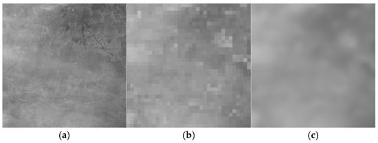
Figure 9. Atmospheric light map. (a) Hazy image. (b) Initial atmospheric light map. (c) Filtered atmospheric light map.

2.4. Transmission Calculation

The initial transmission map is calculated based on the relation equation between the histogram feature and transmission, and the final transmission map is obtained after filtering. The detailed process is described below.

2.4.1. Initial Transmission Map

From Equation (21), the transmission corresponding to the plain image patch in the interval range $(0,1)$ is expressed as follows:

$$t={\displaystyle \frac{k_p(y_p-\sqrt{({y_p}^2-4)})}{2}}.$$

(29)

From Equation (22), the transmission corresponding to the mixed image patch is expressed as follows:

$$t=y_m/k_m.$$

(30)

From Equation (1), the dehazing result of the image patch with index $i$ is expressed as follows:

$$J_p^i(x)={\displaystyle \frac{I_p^i(x)-A_g(x)}{t_p^i(x)}}+A_g(x),$$

(31)

where $x$ represents the position of the pixel in the image, $I_p^i$ represents the hazy image patch with index $i$, $A_g(x)$ denotes the atmospheric light, and $t_p^i$ represents the transmission corresponding to the image patch with index $i$.

From Equation (29), it can be seen that the smaller the value of $k_p$ is, the smaller the transmission $t$ of the image patch is, and the greater the contrast of the dehazed image patch is. However, as the value of $k_p$ decreases, intensity inversion may occur. That is, the intensity of the pixel changes from bright to dark, or from dark to bright. We take values of $k_p$ in descending order from 1.1 to 0.4 with a step size of 0.1, and select 40 plain image patches from the hazy image and perform dehazing according to Equations (29) and (31). These 40 plain image patches include 20 brighter image patches and 20 darker image patches. In brighter image patches, the gray level $I_m^p$ with the highest number of occurrences is greater than the threshold $T_b$, and the value of $T_b$ is set to 150. In darker image patches, the gray level $I_m^p$ with the highest number of occurrences is smaller than the threshold $T_d$, and the value of $T_d$ is set to 80. We calculate the standard deviation ${\sigma }_p$ of the pixel intensity value within the image patch. As $k_p$ decreases, a sequence of ${\sigma }_p^i$($i=1,2,3,\cdots ,8$) is obtained. When $\left|{\sigma }_p^{i+1}-{\sigma }_p^i\right|>T_{inv}$ occurs within an image patch, it indicates intensity inversion, and the current corresponding value of $k_p^i$ is recorded. The final value of $k_p$ is expressed as follows:

$$k_p=k_p^i+0.2.$$

(32)

The standard deviation ${\sigma }_p$ of pixel intensity values is calculated as follows:

$${\sigma }_p=\sqrt{{\displaystyle \frac{1}{N_s}}{\displaystyle \sum _{i=1}^{N_s}{(I_i-\overline{I})}^2}},$$

(33)

where $I_i$ represents the intensity value of the pixel with index $i$ within the image patch, $\overline{I}$ represents the mean of pixel intensity values within the image patch, $N_s$ represents the number of pixels in the image patch. We take values of $k_m$ in increasing order from 16 to 23 with a step size of 0.5, and select 40 mixed image patches from the hazy image and perform dehazing according to Equations (30) and (31). These 40 mixed image patches also include 20 brighter image patches and 20 darker image patches. We calculate the standard deviation ${\sigma }_p$ of the pixel intensity value within the image patch. As $k_m$ increases, a sequence of ${\sigma }_p^i$($i=1,2,3,\cdots ,15$) is obtained. When $\left|{\sigma }_p^{i+1}-{\sigma }_p^i\right|>T_{inv}$ occurs within an image patch, it indicates intensity inversion, and the current corresponding value of $k_m^i$ is recorded. The final value of $k_m$ is denoted as follows:

$$k_m=k_m^i-1.$$

(34)

The initial transmission map is calculated by substituting $k_p$ and $k_m$ into Equation (29) and Equation (30), respectively.

2.4.2. Transmission Map Smoothing

In reality, transmission exhibits smoothness in the spatial domain, i.e., the transmission of any patch is close to the transmission of at least one of its eight-neighborhood patches. If the difference between the transmission of a patch and the transmission of one of its eight-neighborhood patches is less than the threshold $T_e$, the transmission of the patch remains unchanged. Otherwise, the transmission of the patch is set to the average of the transmission of its eight-neighborhood patches. The eight-neighborhood mean filtering of the initial transmission map is defined with the following equation:

$$t_e(i,j)=\left\{\begin{array}{l}t(i,j),if\exists (k,l)\in {\mathrm{N}}_e(i,j),\left|t(i,j)-t(k,l)\right|<T_e;\\ {\displaystyle \frac{1}{8}}{\displaystyle \sum _{(k,l)\in {\mathrm{N}}_e(i,j)}t(k,l),otherwise,}\end{array}\right.,$$

(35)

where $t(i,j)$ denotes the transmission of the image patch located at the $j$-th row and $i$-th column, $N_e(i,j)$ denotes the eight-neighborhood of the image patch at position $(i,j)$. Since the transmission changes slowly in any local neighborhood, Gaussian filtering is used to filter the transmission map after the eight-neighborhood mean filtering, which is expressed as follows:

$$t_g(x,y)=G_{{\sigma }_t}(t_e(x,y)),$$

(36)

where $(x,y)$ represents the position of the pixel in the image, $t_g(x,y)$ denotes the transmission map after Gaussian filtering, $t_e(x,y)$ denotes the transmission map after eight-neighborhood mean filtering. ${\sigma }_t$ is the standard deviation, and the value of ${\sigma }_t$ is set to 14. The transmission map is shown in Figure 10.

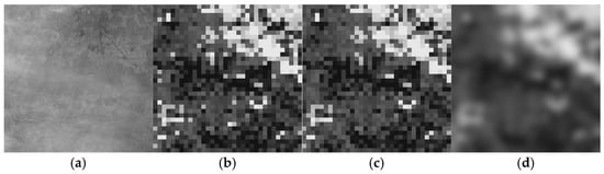
Figure 10. Transmission map. (a) Hazy image. (b) Initial transmission map. (c) Transmission map after eight-neighborhood mean filtering. (d) Transmission map after Gaussian filtering.

2.5. Image Restoration

Transmission is constrained to the range of $[0.1,0.9]$, and the corrected transmission is expressed as follows:

$$t_m(x,y)=\min (0.9,\max (0.1,t_g(x,y))).$$

(37)

From Equation (1), the entire dehazed image is calculated as follows:

$$J(x)={\displaystyle \frac{I(x)-A_g(x)}{t_m(x)}}+A_g(x).$$

(38)

3. Results

To evaluate the effectiveness of the proposed dehazing algorithm, experiments were conducted on the RICE-1 dataset, the RSHaze dataset, and the Jilin-1 dataset. The RICE-1 dataset is one of the most commonly used remote sensing dehazing datasets, containing scenes such as mountains, forests, and cities. The RSHaze dataset is a dataset specifically constructed for remote sensing image dehazing tasks, containing images with different haze densities such as light haze, moderate haze, and dense haze. Both the RICE-1 and RSHaze datasets provide hazy remote sensing images and their corresponding clear reference images. The RICE-1 dataset contains 500 image pairs, while the RSHaze dataset consists of 54,000 image pairs, all with a resolution of 512 × 512 pixels. The hazy panchromatic Jilin-1 satellite images were cropped into 110 images with a resolution of 512 × 512 pixels, forming the Jilin-1 dataset. The Jilin-1 dataset does not have corresponding clear reference images. The test images in the RICE-1 and RSHaze datasets are color images, while the test images in the Jilin-1 dataset are monochrome images. Equation (20) is used to convert the color test images in the RICE-1 and RSHaze datasets into monochrome images. The dehazing performance of the proposed algorithm is compared with algorithms designed for monochrome image dehazing, including DehazeNet [14], AMGAN-CR [20], and MS-GAN [21], and the work of Jang et al. [55], Khan et al. [56], Singh et al. [49], and Ding et al. [34]. The dehazing algorithms were run on hardware environments with an Intel Core i7-1165G7 CPU or an NVIDIA GeForce RTX 3080Ti GPU.

3.1. Qualitative Evaluation

The proposed dehazing algorithm was tested on the RICE-1 dataset, the RSHaze dataset, and the Jilin-1 dataset. The test images included thin haze images, dense haze images, and uneven haze images. The dehazing results are shown in Figure 11, Figure 12 and Figure 13.

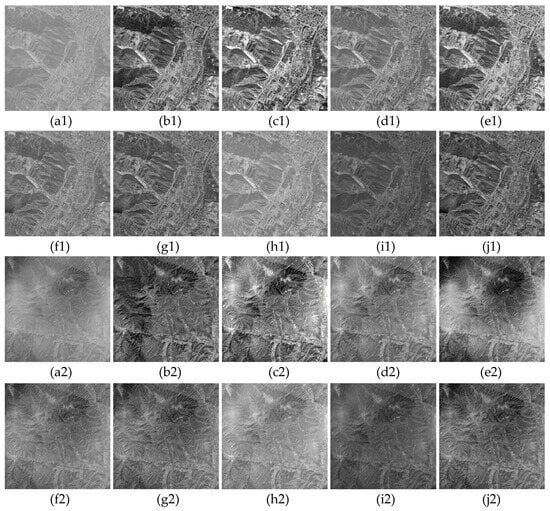
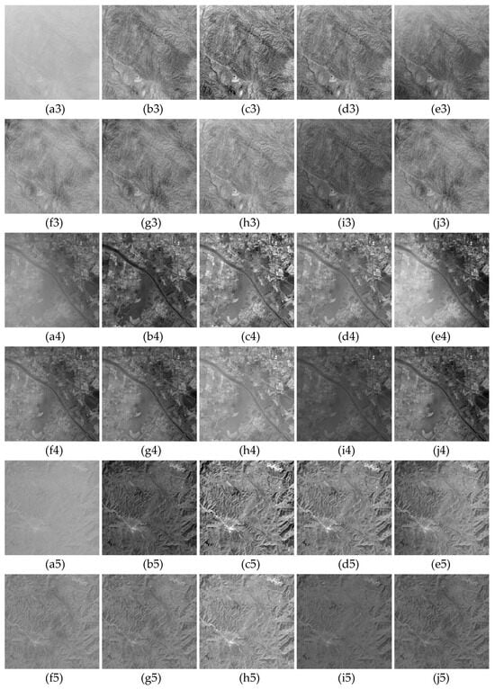
Figure 11. Dehazing results on the RICE-1 dataset. (a1–a5) Hazy images. (b1–b5) Clear reference images. (c1–c5) The work of Jang et al. [55]. (d1–d5) The work of Khan et al. [56]. (e1–e5) The work of Singh et al. [49]. (f1–f5) DehazeNet [14]. (g1–g5) The work of Ding et al. [34]. (h1–h5) AMGAN-CR [20]. (i1–i5) MS-GAN [21]. (j1–j5) The proposed algorithm.

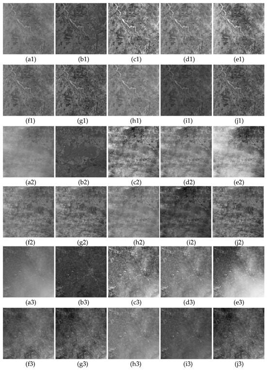
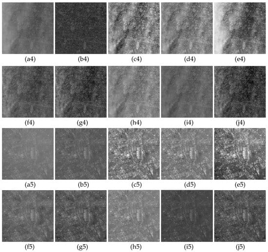
Figure 12. Dehazing results on the RSHaze dataset. (a1–a5) Hazy images. (b1–b5) Clear reference images. (c1–c5) The work of Jang et al. [55]. (d1–d5) the work of Khan et al. [56]. (e1–e5) The work of Singh et al. [49]. (f1–f5) DehazeNet [14]. (g1–g5) The work of Ding et al. [34]. (h1–h5) AMGAN-CR [20]. (i1–i5) MS-GAN [21]. (j1–j5) The proposed algorithm.

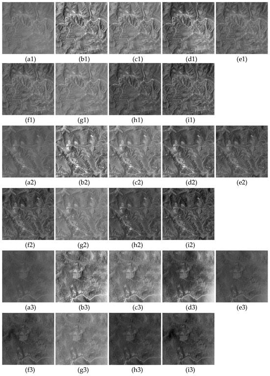
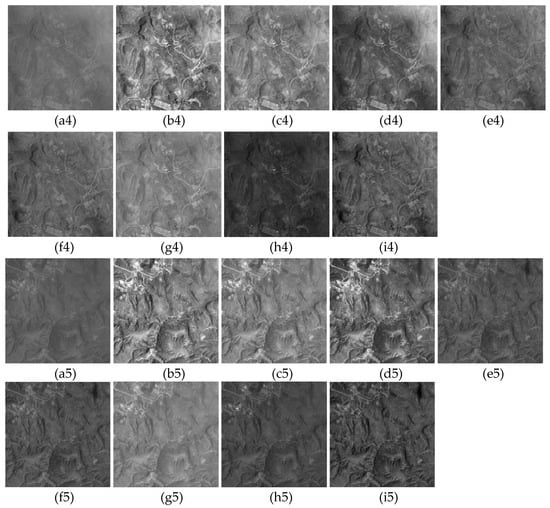
Figure 13. Dehazing results on the Jilin-1 dataset. (a1–a5) Hazy images. (b1–b5) The work of Jang et al. [55]. (c1–c5) The work of Khan et al. [56]. (d1–d5) The work of Singh et al. [49]. (e1–e5) DehazeNet [14]. (f1–f5) The work of Ding et al. [34]. (g1–g5) AMGAN-CR [20]. (h1–h5) MS-GAN [21]. (i1–i5) The proposed algorithm.

Figure 11 demonstrates the qualitative results on the RICE-1 dataset. Jang et al. [55] achieve high contrast in the dehazed images, but local image regions exhibit oversaturation, as shown in the left-middle portion of Figure 11(c1). Additionally, the dehazing effect is incomplete for uneven haze images, as illustrated in the left-upper portion of Figure 11(c2). The algorithms proposed by Khan et al. [56] and Singh et al. [49] perform poorly on images with uneven haze, as shown in the left-upper part of Figure 11(d2,e2). DehazeNet [14], AMGAN-CR [20], and MS-GAN [21] produce overall low-contrast dehazed images, failing to completely remove the haze. Ding et al. [34] fail to completely remove haze from dense hazy images, as shown in Figure 11(g5). The proposed algorithm achieves good dehazing results for thin haze, dense haze, and uneven haze images, with the dehazed images being closer to the clear reference images.

Figure 12 shows the visual comparison on the RSHaze dataset. The algorithms of Jang et al. [55], Khan et al. [56], and the AMGAN-CR algorithm [20] achieve unsatisfactory dehazing results for dense haze images, as shown in the middle part of Figure 12(c2,d2,h2). The work of Singh et al. [49] and the MS-GAN algorithm [21] achieve poor dehazing results for uneven haze images, as shown in the left part of Figure 12(e4,i4). DehazeNet [14] and the work of Ding et al. [34] also produce unsatisfactory results for dense haze images, as shown in Figure 12(f5,g5). The proposed algorithm achieves pleasing dehazing results for various types of hazy images, with the dehazed images exhibiting uniform brightness and high contrast.

Figure 13 shows the qualitative results on the real panchromatic Jilin-1 dataset. An oversaturation artifact is observed in the dehazing result of Jang et al. [55], as shown in the left-upper portion of Figure 13(b5). The work of Khan et al. [56], Singh et al. [49], and the AMGAN-CR algorithm [20] achieve poor dehazing results for images with uneven haze, as demonstrated in the right-lower portions of Figure 13(c3,d3,g3). DehazeNet [14], the work of Ding et al. [34], and MS-GAN [21] produce low contrast dehazed images, as shown in Figure 13(e4,f4,h4). The proposed dehazing algorithm effectively calculates the transmission of each local region in the hazy image, achieving satisfactory dehazing results.

3.2. Quantitative Evaluation

PSNR [64], SSIM [65], RMSC [66], and the rate of new visible edges $e$ [67] are used to evaluate the image quality of the dehazed images. PSNR and SSIM are reference-based image quality evaluation methods, while RMSC and the rate of new visible edges $e$ are no-reference image quality evaluation methods.

PSNR is a widely used objective metric for assessing the quality of restored images, measuring restoration accuracy by calculating the pixel-level error between the restored image and the reference image. A higher PSNR value indicates better image quality. PSNR is calculated based on mean squared error (MSE), which represents the mean squared error between all pixels in the two images. The MSE is defined as follows:

$$\mathrm{MSE}={\displaystyle \frac{1}{MN}}{\displaystyle \sum _{i=1}^M{\displaystyle \sum _{j=1}^N{(I_r(i,j)-I_d(i,j))}^2}},$$

(39)

where $(i,j)$ represents the position of the pixel in the image, $I_r$ represents the clear reference image, $I_d$ represents the dehazed image, $M$ and $N$ represent the width and height of the image, respectively. The PSNR is calculated as follows:

$$PSNR=10\cdot {\log }_{10}({\displaystyle \frac{{I_{L-1}}^2}{MSE}}),$$

(40)

where $I_{L-1}$ represents the maximum gray level of the image.

SSIM is an image quality evaluation index based on the human visual system (HVS) that measures the similarity between a restored image and a reference image in terms of three dimensions: luminance, contrast, and structure. The higher the SSIM value, the better the image quality. The SSIM index between image $x$ and $y$ is defined as follows:

$$SSIM(x,y)={\displaystyle \frac{(2{\mu }_x{\mu }_y+C_1)(2{\sigma }_{xy}+C_2)}{({{\mu }_x}^2+{{\mu }_y}^2+C_1)({{\sigma }_x}^2+{{\sigma }_y}^2+C_2)}},$$

(41)

where ${\mu }_x$ and ${\mu }_y$ represent the mean values of image $x$ and $y$, respectively. ${\sigma }_x$ and ${\sigma }_y$ represent the standard deviations of image $x$ and $y$, respectively. ${\sigma }_{xy}$ represents the covariance between image $x$ and $y$, and $C_1$ and $C_2$ are constants.

RMSC calculates the contrast of the dehazed image based on the root mean square of the image intensity values. The larger the RMSC value, the better the image quality. The definition of RMSC is as follows:

$${\overline{C}}_k={\displaystyle \frac{1}{N_b}}{\displaystyle \sum _{k=1}^{N_b}{C}_k},$$

(42)

$$C_k=\sqrt{{\displaystyle \frac{1}{N_s}}{\displaystyle \sum _{i=1}^{N_s}{(I_k^i-{\overline{I}}_k)}^2}},$$

(43)

where ${\overline{C}}_k$ represents the mean RMSC of all image patches, $C_k$ represents the RMSC of the $k$-th image patch, $N_b$ represents the number of image patches, $I_k^i$ denotes the intensity of the $i$-th pixel in the $k$-th image block, ${\overline{I}}_k$ denotes the mean intensity of pixels in the $k$-th image patch, and $N_s$ denotes the number of pixels in the image patch.

$e$ reflects the change in the visible edges of the image before and after dehazing. The larger the value of $e$, the better the dehazing effect. $e$ is defined as follows:

$$e={\displaystyle \frac{n_r-n_o}{n_o}},$$

(44)

where $n_r$ and $n_o$ represent the number of visible edges in the dehazed image and hazy image, respectively.

The average results of quantitative evaluation metrics for different dehazing algorithms on different datasets are shown in Table 1.

Table 1. The average results of quantitative evaluation metrics.

Method	RICE-1				RSHaze				Jilin-1
	PSNR	SSIM	RMSC	e	PSNR	SSIM	RMSC	e	RMSC	e
Jang et al. [55]	19.53	0.76	25.69	0.11	17.42	0.72	24.05	0.13	22.61	0.07
Khan et al. [56]	23.79	0.80	19.46	0.13	20.77	0.78	17.16	0.12	17.83	0.09
Singh et al. [49]	16.83	0.71	22.18	0.08	15.97	0.67	15.71	0.07	19.42	0.06
DehazeNet [14]	27.04	0.85	17.93	0.19	25.29	0.83	19.86	0.15	16.08	0.13
Ding et al. [34]	28.51	0.87	20.59	0.24	27.62	0.85	21.19	0.19	16.94	0.16
AMGAN-CR [20]	19.26	0.78	19.84	0.10	18.61	0.74	16.86	0.09	16.62	0.11
MS-GAN [21]	22.74	0.82	20.18	0.15	26.57	0.81	18.37	0.12	17.16	0.12
Proposed	31.73	0.91	23.74	0.32	29.48	0.89	23.94	0.26	20.96	0.19

Bold numbers are used to highlight which result is the best in the column. Underlined numbers are used to highlight which result is the second-best in the column.

As shown in Table 1, for the RICE-1 and RSHaze datasets with reference images, the proposed algorithm achieves the best PSNR, SSIM, and $e$ evaluation metrics. The images restored by the proposed algorithm are closest to the reference images. For the Jilin-1 dataset without reference images, the proposed algorithm achieves the best $e$ evaluation metric. For the RMSC metric across the three datasets, the method proposed by Jang et al. [55] is the optimal one, while the proposed algorithm is the second-best. Although the method proposed by Jang et al. [55] enhances the contrast of the dehazed images, it results in the loss of detail information, as evidenced by the PSNR, SSIM, and $e$ evaluation metrics.

3.3. Ablation Experiment

3.3.1. Validity of Atmospheric Light Calculation

We proposed a threshold segmentation approach to calculate the atmospheric light for each image patch based on its maximum gray level. To demonstrate the validity of our calculation method, the proposed approach is compared with a method that assigns a single atmospheric light value to the entire image. For the comparison method, we calculate the atmospheric light as the average intensity of the top 0.1 percent brightest pixels in the hazy image. All other steps and parameters of the comparison algorithm HF_a1 remained identical to the proposed algorithm. Both the proposed algorithm and HF_a1 were tested on the RICE-1 and RSHaze datasets and the experimental results are shown in Figure 14 and Table 2. Row 1 in Figure 14 shows the results on the RICE-1 dataset, while Row 2 shows the results on the RSHaze dataset. As evident from the middle portion of the first image and the lower part of the second image in Figure 14c, the dehazed images produced by HF_a1 exhibit dark local regions and uneven brightness. In contrast, the images dehazed by our proposed algorithm demonstrate uniform brightness. Table 2 shows that the PSNR and SSIM of the dehazed images from HF_a1 are significantly lower than those from the proposed algorithm.

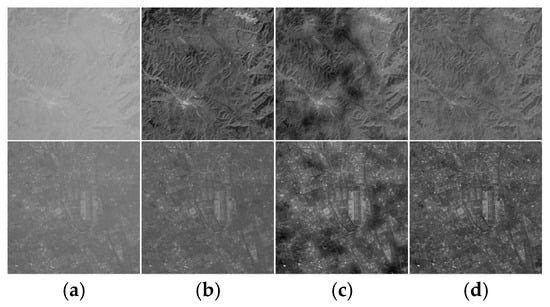
Figure 14. Dehazing results using different atmospheric light calculation methods. (a) Hazy images. (b) Clear reference images. (c) HE_a1 algorithm. (d) Proposed algorithm.

Table 2. The average results of quantitative evaluation metrics using different atmospheric light calculation methods.

Method	RICE-1		RSHaze
	PSNR	SSIM	PSNR	SSIM
HE_a1	20.92	0.81	19.24	0.78
Proposed	31.73	0.91	29.48	0.89

3.3.2. Influence of Patch Classification Threshold $T_m$

To illustrate the impact of the patch classification threshold $T_m$, we perform four experiments with $T_m$ set to 0.45, 0.55, 0.65, and 0.75, respectively. Only the threshold $T_m$ differs across these four experiments and all other steps and parameters remain identical. The experimental results are shown in Figure 15 and Table 3. Figure 15 shows that the contrast increases sequentially from (c) to (f), with oversaturation appearing in the right part of (f). Table 3 indicates that when $T_m=0.65$, the PSNR and SSIM reach their maximum. To achieve optimal dehazing results, we set $T_m$ to 0.65.

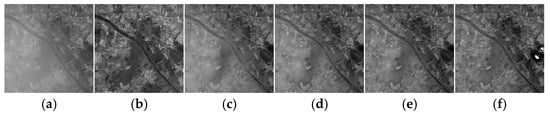
Figure 15. Experimental results with different patch classification threshold $T_m$. (a) Hazy image. (b) Clear reference image. (c) $T_m=0.45$. (d) $T_m=0.55$. (e) $T_m=0.65$. (f) $T_m=0.75$.

Table 3. The average results of quantitative evaluation metrics with different patch classification threshold $T_m$.

$${\mathit{T}}_{\mathit{m}}$$	RICE-1		RSHaze
	PSNR	SSIM	PSNR	SSIM
0.45	26.93	0.83	26.31	0.82
0.55	27.38	0.86	27.19	0.84
0.65	31.73	0.91	29.48	0.89
0.75	25.39	0.82	24.57	0.79

Bold numbers are used to highlight which result is the best in the column.

3.4. Running Time

The dehazing algorithms are executed on a hardware platform equipped with an Intel Core i7-1165G7 CPU and an NVIDIA GeForce RTX 3080 Ti GPU. The algorithms proposed by Jang et al. [55], Khan et al. [56], and Singh et al. [49], and the proposed algorithm were run on the CPU, denoted as (C) in Table 4. The algorithms proposed by DehazeNet [14], Ding et al. [34], AMGAN-CR [20], and MS-GAN [21] were run on the GPU, denoted as (G) in Table 4. Experiments were conducted on images with a resolution of 512 × 512 from the RICE-1, RSHaze, and Jilin-1 datasets, and the average running times of the dehazing algorithms are shown in Table 4.

Table 4. The average running time (seconds) of the dehazing algorithms.

Methods	Time
Jang et al. [55]	0.25 (C)
Khan et al. [56]	0.48 (C)
Singh et al. [49]	0.32 (C)
DehazeNet [14]	0.29 (G)
Ding et al. [34]	0.36 (G)
AMGAN-CR [20]	0.38(G)
MS-GAN [21]	0.27(G)
Proposed	0.21 (C)

Bold numbers are used to highlight which result is the best in the column. Underlined numbers are used to highlight which result is the second-best in the column.

As shown in Table 4, the proposed algorithm has the highest running efficiency, with an average execution time of only 0.21 s. The proposed algorithm can be executed without relying on high-performance hardware platforms such as GPUs.

4. Discussion

In this paper, we classified hazy images into plain image patches and mixed image patches based on histogram features. We innovatively propose calculation methods for the AODAG features of plain image patches and the ADGG features of mixed image patches. Through statistical analysis, we derived the relation equation between AODAG features and transmission, as well as the relation equation between ADGG features and transmission. Transmission can be calculated by using these two relation equations and the dehazed image can be obtained via the atmosphere scattering model. Experiments on synthetic and real datasets demonstrated that images processed by the proposed dehazed algorithm appear more natural and closely resemble clear images.

The proposed algorithm is not suitable for haze removal in nighttime light remote sensing images due to the following reasons: (1) The proposed algorithm utilizes an atmosphere scattering model for dehazing, in which the sun is the only light source. Nighttime hazy images typically contain multiple light sources such as streetlights, causing the model-based dehazing algorithm to fail. (2) The histogram features of image patches only manifest under conditions of relatively uniform ambient illumination. However, nighttime hazy images exhibit significant variations in ambient illumination across different regions, causing the histogram features of image patches to disappear. In order to make the histogram features applicable to nighttime image dehazing, the atmosphere scattering model must be modified to accommodate multiple light sources. Concurrently, research is needed on the relationship between histogram features and transmission under non-uniform illumination conditions.

5. Conclusions

For panchromatic remote sensing images lacking color information, we innovatively proposed an image dehazing method based on histogram features. The proposed algorithm establishes the relation equation between the AODAG features and transmission of plain image patches, as well as the relation equation between the ADGG features and transmission of mixed image patches. According to the characteristics of atmospheric light distribution in remote sensing images, a threshold segmentation method was employed to calculate the atmospheric light corresponding to each image patch based on the maximum gray level within the image patch. Qualitative and quantitative evaluation metrics demonstrate that the dehazing performance of the proposed algorithm outperforms the five comparison algorithms. The proposed algorithm also exhibits satisfactory computational efficiency and can be implemented on a standard CPU hardware platform.

References

- Li, Z.; Leung, H. Fusion of multispectral and panchromatic images using a restoration-based method. IEEE Trans. Geosci. Remote Sens. 2009, 47, 1482–1491. [Google Scholar]
- Nie, J.; Xie, J.; Sun, H. Remote Sensing Image Dehazing via a Local Context-Enriched Transformer. Remote Sens. 2024, 16, 1422. [Google Scholar] [CrossRef]
- Han, S.; Ngo, D.; Choi, Y.; Kang, B. Autonomous Single-Image Dehazing: Enhancing Local Texture with Haze Density-Aware Image Blending. Remote Sens. 2024, 16, 3641. [Google Scholar] [CrossRef]
- He, K.; Sun, J.; Tang, X. Single image haze removal using dark channel prior. In Proceedings of the IEEE/CVF Conference Computer Vision and Pattern Recognition (CVPR), Miami, FL, USA, 20–25 June 2009; pp. 1956–1963. [Google Scholar]
- Wang, A.; Wang, W.; Liu, J.; Gu, N. AIPNet: Image-to-image single image dehazing with atmospheric illumination prior. IEEE Trans. Image Process. 2018, 28, 381–393. [Google Scholar] [CrossRef]
- Qiu, Z.; Gong, T.; Liang, Z.; Chen, T.; Cong, R.; Bai, H.; Zhao, Y. Perception-oriented UAV image dehazing based on super-pixel scene prior. IEEE Trans. Geosci. Remote Sens. 2024, 62, 5913519. [Google Scholar] [CrossRef]
- Wang, W.; Wang, A.; Liu, C. Variational single nighttime image haze removal with a gray haze-line prior. IEEE Trans. Image Process. 2022, 31, 1349–1363. [Google Scholar] [CrossRef] [PubMed]
- Ling, P.; Chen, H.; Tan, X.; Jin, Y.; Chen, E. Single image dehazing using saturation line prior. IEEE Trans. Image Process. 2023, 32, 3238–3253. [Google Scholar] [CrossRef]
- Zhu, Q.; Mai, J.; Shao, L. A fast single image haze removal algorithm using color attenuation prior. IEEE Trans. Image Process. 2015, 24, 3522–3533. [Google Scholar] [CrossRef]
- Bi, G.; Si, G.; Zhao, Y.; Qi, B.; Lv, H. Haze removal for a single remote sensing image using low-rank and sparse prior. IEEE Trans. Geosci. Remote Sens. 2021, 60, 5615513. [Google Scholar] [CrossRef]
- Liu, J.; Wen Liu, R.; Sun, J.; Zeng, T. Rank-one prior: Toward real-time scene recovery. In Proceedings of the IEEE/CVF Conference Computer Vision and Pattern Recognition (CVPR), Nashville, TN, USA, 10–25 June 2021; pp. 14797–14805. [Google Scholar]
- Zhang, X.; Wang, T.; Tang, G.; Zhao, L.; Xu, Y.; Maybank, S. Single image haze removal based on a simple additive model with haze smoothness prior. IEEE Trans. Circuits Syst. Video Technol. 2021, 32, 3490–3499. [Google Scholar] [CrossRef]
- Tan, Y.; Zhu, Y.; Huang, Z.; Tan, H.; Li, K. MAPD: An FPGA-based real-time video haze removal accelerator using mixed atmosphere prior. IEEE Trans. Comput.-Aided Des. Integr. Circuits Syst. 2023, 42, 4777–4790. [Google Scholar] [CrossRef]
- Cai, B.; Xu, X.; Jia, K.; Qing, C.; Tao, D. Dehazenet: An end-to-end system for single image haze removal. IEEE Trans. Image Process. 2016, 25, 5187–5198. [Google Scholar] [CrossRef]
- Li, B.; Peng, X.; Wang, Z.; Xu, J.; Feng, D. AOD-Net: All-in-one dehazing network. In Proceedings of the IEEE Internation Conference Computer Vision (ICCV), Venice, Italy, 22–29 October 2017; pp. 4780–4788. [Google Scholar]
- Zhu, X.; Li, S.; Gan, Y.; Zhang, Y.; Sun, B. Multi-stream fusion network with generalized smooth L1 loss for single image dehazing. IEEE Trans. Image Process. 2021, 30, 7620–7635. [Google Scholar] [CrossRef]
- Liu, X.; Ma, Y.; Shi, Z.; Chen, J. GriddehazeNet: Attention-based multi-scale network for image dehazing. In Proceedings of the IEEE Internation Conference Computer Vision (ICCV), Seoul, Republic of Korea, 27 October–2 November 2019; pp. 7313–7322. [Google Scholar]
- Wu, P.; Pan, Z.; Tang, H.; Hu, Y. Cloudformer: A cloud-removal network combining self-attention mechanism and convolution. Remote Sens. 2022, 14, 6132. [Google Scholar] [CrossRef]
- Yeh, C.; Huang, C.; Kang, L. Multi-scale deep residual learning-based single image haze removal via image decomposition. IEEE Trans. Image Process. 2019, 29, 3153–3167. [Google Scholar] [CrossRef] [PubMed]
- Xu, M.; Deng, F.; Jia, S.; Jia, X.; Plaza, A. Attention mechanism-based generative adversarial networks for cloud removal in Landsat images. Remote Sens. Environ. 2022, 271, 112902. [Google Scholar] [CrossRef]
- Xu, Z.; Wu, K.; Huang, L.; Wang, Q.; Ren, P. Cloudy image arithmetic: A cloudy scene synthesis paradigm with an application to deep-learning-based thin cloud removal. IEEE Trans. Geosci. Remote Sens. 2022, 60, 5612616. [Google Scholar] [CrossRef]
- Sun, H.; Luo, Z.; Ren, D.; Du, B.; Chang, L.; Wan, J. Unsupervised multi-branch network with high-frequency enhancement for image dehazing. Pattern Recognit. 2024, 156, 110763. [Google Scholar] [CrossRef]
- Chen, X.; Li, Y.; Kong, C.; Dai, L. Unpaired image dehazing with physical-guided restoration and depth-guided refinement. IEEE Signal Process. Lett. 2022, 29, 587–591. [Google Scholar] [CrossRef]
- Zheng, Y.; Su, J.; Zhang, S.; Tao, M.; Wang, L. Dehaze-AGGAN: Unpaired remote sensing image dehazing using enhanced attention-guide generative adversarial networks. IEEE Trans. Geosci. Remote Sens. 2022, 60, 5630413. [Google Scholar] [CrossRef]
- Ullah, H.; Muhammad, K.; Irfan, M.; Anwar, S.; Sajjad, M.; Imran, A.; Albuquerque, V. Light-DehazeNet: A novel lightweight CNN architecture for single image dehazing. IEEE Trans. Image Process. 2021, 30, 8968–8982. [Google Scholar] [CrossRef]
- Zhang, Y.; Wang, X.; Bi, X.; Tao, D. A light dual-task neural network for haze removal. IEEE Signal Process. Lett. 2018, 25, 1231–1235. [Google Scholar] [CrossRef]
- Li, S.; Zhou, Y.; Kung, S. PSRNet: A progressive self-refine network for lightweight optical remote sensing image dehazing. IEEE Trans. Geosci. Remote Sens. 2024, 62, 5648413. [Google Scholar] [CrossRef]
- Cai, Z.; Ning, J.; Ding, Z.; Duo, B. Additional self-attention transformer with adapter for thick haze removal. IEEE Geosci. Remote Sens. Lett. 2024, 21, 6004705. [Google Scholar] [CrossRef]
- Song, T.; Fan, S.; Li, P.; Jin, J.; Jin, G.; Fan, L. Learning an effective transformer for remote sensing satellite image dehazing. IEEE Geosci. Remote Sens. Lett. 2023, 20, 8002305. [Google Scholar] [CrossRef]
- Ning, J.; Yin, J.; Deng, F.; Xie, L. MABDT: Multi-scale attention boosted deformable transformer for remote sensing image dehazing. Signal Process. 2024, 229, 109768. [Google Scholar] [CrossRef]
- Dong, H.; Song, T.; Qi, X.; Jin, G.; Jin, J.; Ma, L. Prompt-guided sparse transformer for remote sensing image dehazing. IEEE Geosci. Remote Sens. Lett. 2024, 21, 8003505. [Google Scholar] [CrossRef]
- Zhang, X.; Xie, F.; Ding, H.; Yan, S.; Shi, Z. Proxy and cross-stripes integration transformer for remote sensing image dehazing. IEEE Trans. Geosci. Remote Sens. 2024, 62, 5640315. [Google Scholar] [CrossRef]
- Sun, H.; Zhong, Q.; Du, B.; Tu, Z.; Wan, J.; Wang, W.; Ren, D. Bidirectional-modulation frequency-heterogeneous network for remote sensing image dehazing. IEEE Trans. Circuits Syst. Video Technol. 2025. [Google Scholar] [CrossRef]
- Ding, H.; Xie, F.; Qiu, L.; Zhang, X.; Shi, Z. Robust haze and thin cloud removal via conditional variational autoencoders. IEEE Trans. Geosci. Remote Sens. 2024, 62, 5604616. [Google Scholar] [CrossRef]
- Ma, X.; Wang, Q.; Tong, X. Nighttime light remote sensing image haze removal based on a deep learning model. Remote Sens. Environ. 2025, 318, 114575. [Google Scholar] [CrossRef]
- Chen, W.; Fang, H.; Ding, J.; Kuo, S. PMHLD: Patch map-based hybrid learning DehazeNet for single image haze removal. IEEE Trans. Image Process. 2020, 29, 6773–6788. [Google Scholar] [CrossRef]
- Zhao, S.; Zhang, L.; Shen, Y.; Zhou, Y. RefineDNet: A weakly supervised refinement framework for single image dehazing. IEEE Trans. Image Process. 2021, 30, 3391–3404. [Google Scholar] [CrossRef] [PubMed]
- Zhang, Y.; Zhou, S.; Li, H. Depth information assisted collaborative mutual promotion network for single image dehazing. In Proceedings of the IEEE/CVF Conference Computer Vision Pattern Recognition (CVPR), Seattle, WA, USA, 17–21 June 2024; pp. 2846–2855. [Google Scholar]
- Wang, Q.; Ward, R. Fast image/video contrast enhancement based on weighted thresholded histogram equalization. IEEE Trans. Consum. Electron. 2007, 53, 757–764. [Google Scholar] [CrossRef]
- Kim, Y. Contrast enhancement using brightness preserving bi-histogram equalization. IEEE Trans. Consum. Electron. 1997, 43, 1–8. [Google Scholar] [CrossRef]
- Celik, T. Spatial entropy-based global and local image contrast enhancement. IEEE Trans. Image Process. 2014, 23, 5298–5308. [Google Scholar] [CrossRef]
- Wu, H.; Cao, X.; Jia, R.; Cheung, Y. Reversible data hiding with brightness preserving contrast enhancement by two-dimensional histogram modification. IEEE Trans. Circuits Syst. Video Technol. 2022, 32, 7605–7617. [Google Scholar] [CrossRef]
- Kim, W.; You, J.; Jeong, J. Contrast enhancement using histogram equalization based on logarithmic mapping. Opt. Eng. 2012, 51, 067002. [Google Scholar] [CrossRef]
- Liu, S.; Lu, Q.; Dai, S. Adaptive histogram equalization framework based on new visual prior and optimization model. Signal Process. Image Commun. 2025, 132, 117246. [Google Scholar] [CrossRef]
- Xu, C.; Peng, Z.; Hu, X.; Zhang, W.; Chen, L.; An, F. FPGA-based low-visibility enhancement accelerator for video sequence by adaptive histogram equalization with dynamic clip-threshold. IEEE Trans. Circuits Syst. I 2020, 67, 3954–3964. [Google Scholar] [CrossRef]
- Wu, X.; Kawanishi, T.; Kashino, K. Reflectance-guided histogram equalization and comparametric approximation. IEEE Trans. Circuits Syst. Video Technol. 2021, 31, 863–876. [Google Scholar] [CrossRef]
- Guo, J.; Syue, J.; Radzicki, V.; Lee, H. An efficient fusion-based defogging. IEEE Trans. Image Process. 2017, 26, 4217–4228. [Google Scholar] [CrossRef]
- Hong, S.; Kim, M.; Kang, M. Single image dehazing via atmospheric scattering model-based image fusion. Signal Process. 2020, 178, 107798. [Google Scholar] [CrossRef]
- Singh, K.; Parihar, A. Variational optimization based single image dehazing. J. Vis. Commun. Image Represent. 2021, 79, 103241. [Google Scholar] [CrossRef]
- Ding, X.; Liang, Z.; Wang, Y.; Fu, X. Depth-aware total variation regularization for underwater image dehazing. Signal Process. Image Commun. 2021, 98, 116408. [Google Scholar] [CrossRef]
- Meng, G.; Wang, Y.; Duan, J.; Xiang, S.; Pan, C. Efficient image dehazing with boundary constraint and contextual regularization. In Proceedings of the IEEE Internation Conference Computer Vision (ICCV), Sydney, NSW, Australia, 1–8 December 2013; pp. 617–624. [Google Scholar]
- Liu, Y.; Wang, X.; Hu, E.; Wang, A.; Shiri, B.; Lin, W. VNDHR: Variational single nighttime image dehazing for enhancing visibility in intelligent transportation systems via hybrid regularization. IEEE Trans. Intell. Transp. Syst. 2025, 26, 10189–10203. [Google Scholar] [CrossRef]
- Liu, Y.; Yan, Z.; Tan, J.; Li, Y. Multi-purpose oriented single nighttime image haze removal based on unified variational Retinex model. IEEE Trans. Circuits Syst. Video Technol. 2022, 33, 1643–1657. [Google Scholar] [CrossRef]
- Liu, Q.; Gao, X.; He, L.; Lu, W. Single image dehazing with depth-aware non-local total variation regularization. IEEE Trans. Image Process. 2018, 27, 5178–5191. [Google Scholar] [CrossRef]
- Jang, J.; Kim, S.; Ra, J. Enhancement of optical remote sensing images by subband-decomposed multiscale Retinex with hybrid intensity transfer function. IEEE Geosci. Remote Sens. Lett. 2011, 8, 983–987. [Google Scholar] [CrossRef]
- Khan, H.; Sharif, M.; Bibi, N.; Usman, M.; Haider, S.; Zainab, S.; Shah, J.; Bashir, Y.; Muhammad, N. Localization of radiance transformation for image dehazing in wavelet domain. Neurocomputing 2019, 381, 141–151. [Google Scholar] [CrossRef]
- Nayar, S.; Narasimhan, S. Vision in bad weather. In Proceedings of the IEEE Internation Conference Computer Vision (ICCV), Corfu, Greece, 20–27 September 1999; pp. 820–827. [Google Scholar]
- Narasimhan, S.G.; Nayar, S.K. Contrast restoration of weather degraded images. IEEE Trans. Pattern Anal. Mach. Intell. 2003, 25, 713–724. [Google Scholar] [CrossRef]
- Gu, Z.; Zhan, Z.; Yuan, Q.; Yan, L. Single remote sensing image dehazing using a prior-based dense attentive network. Remote Sens. 2019, 11, 3008. [Google Scholar] [CrossRef]
- Zhang, L.; Wang, S. Dense haze removal based on dynamic collaborative inference learning for remote sensing images. IEEE Trans. Geosci. Remote Sens. 2022, 60, 5631016. [Google Scholar] [CrossRef]
- Lin, D.; Xu, G.; Wang, X.; Wang, Y.; Sun, X.; Fu, K. A remote sensing image dataset for cloud removal. arXiv 2019, arXiv:1901.00600. [Google Scholar] [CrossRef]
- Song, Y.; He, Z.; Qian, H.; Du, X. Vision transformers for single image dehazing. arXiv 2022, arXiv:2204.03883. [Google Scholar] [CrossRef]
- Pilanci, M.; Arikan, O.; Pinar, M. Structured least squares problems and robust estimators. IEEE Trans. Signal Process. 2010, 58, 2453–2465. [Google Scholar] [CrossRef]
- Huynh-Thu, Q.; Ghanbari, M. Scope of validity of PSNR in image/video quality assessment. Electron. Lett. 2008, 44, 800–808. [Google Scholar] [CrossRef]
- Wang, Z.; Bovik, A.; Sheikh, H.; Simoncelli, E. Image quality assessment: From error visibility to structural similarity. IEEE Trans. Image Process. 2004, 13, 600–612. [Google Scholar] [CrossRef]
- Xie, X.; Yu, C. Perceptual learning of Vernier discrimination transfers from high to zero noise after double training. Vision Res. 2019, 156, 39–45. [Google Scholar] [CrossRef] [PubMed]
- Hautiere, N.; Tarel, J.P.; Aubert, D.; Dumont, E. Blind contrast enhancement assessment by gradient ratioing at visible edges. Image Anal. Stereol. 2008, 27, 87–95. [Google Scholar] [CrossRef]
Disclaimer/Publisher’s Note: The statements, opinions and data contained in all publications are solely those of the individual author(s) and contributor(s) and not of MDPI and/or the editor(s). MDPI and/or the editor(s) disclaim responsibility for any injury to people or property resulting from any ideas, methods, instructions or products referred to in the content. |
© 2025 by the authors. Licensee MDPI, Basel, Switzerland. This article is an open access article distributed under the terms and conditions of the Creative Commons Attribution (CC BY) license (https://creativecommons.org/licenses/by/4.0/).