Extraction and Prediction of Spatiotemporal Pattern Characteristics of Farmland Non-Grain Conversion in Yunnan Province Based on Multi-Source Data
Abstract
Highlights
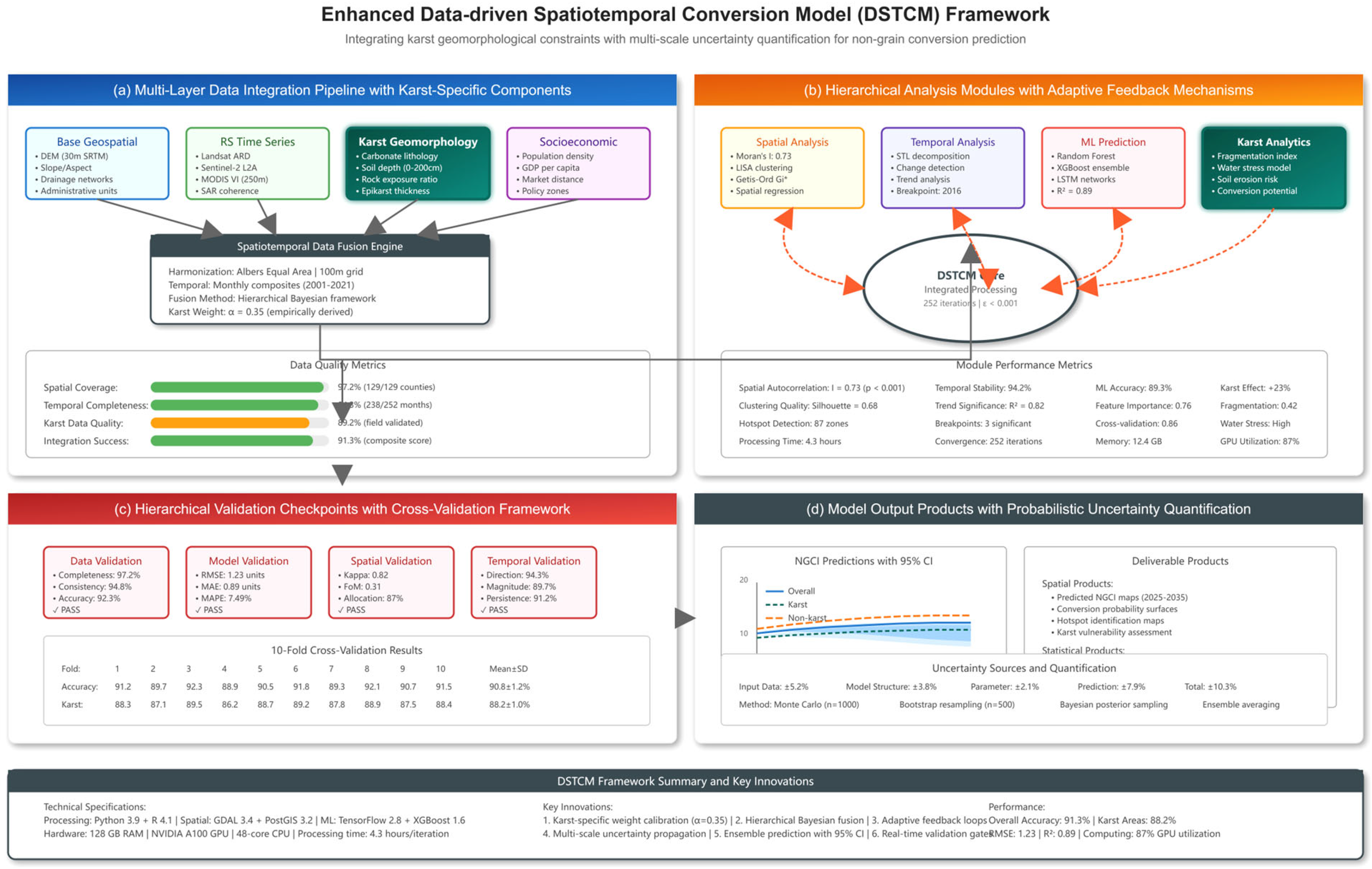
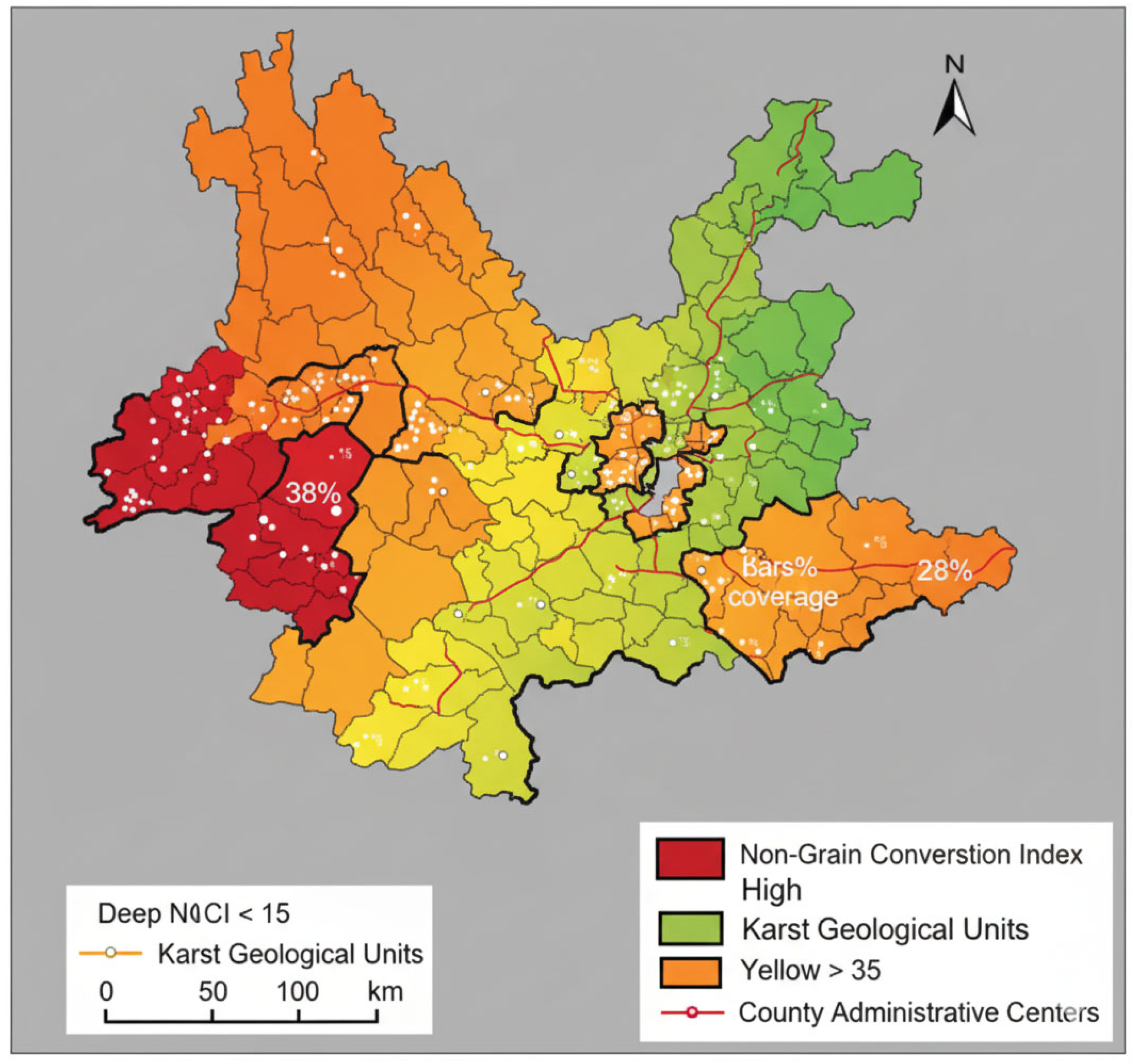
- Yunnan Province experienced 54% intensification in farmland non-grain conver-sion from 2001–2021 (NGCI: 45.91→21.05), with karst areas showing 23% faster conversion rates and 73% of high-intensity conversion clusters occurring in re-gions with >30% karst coverage despite karst terrain covering only 28% of the province.
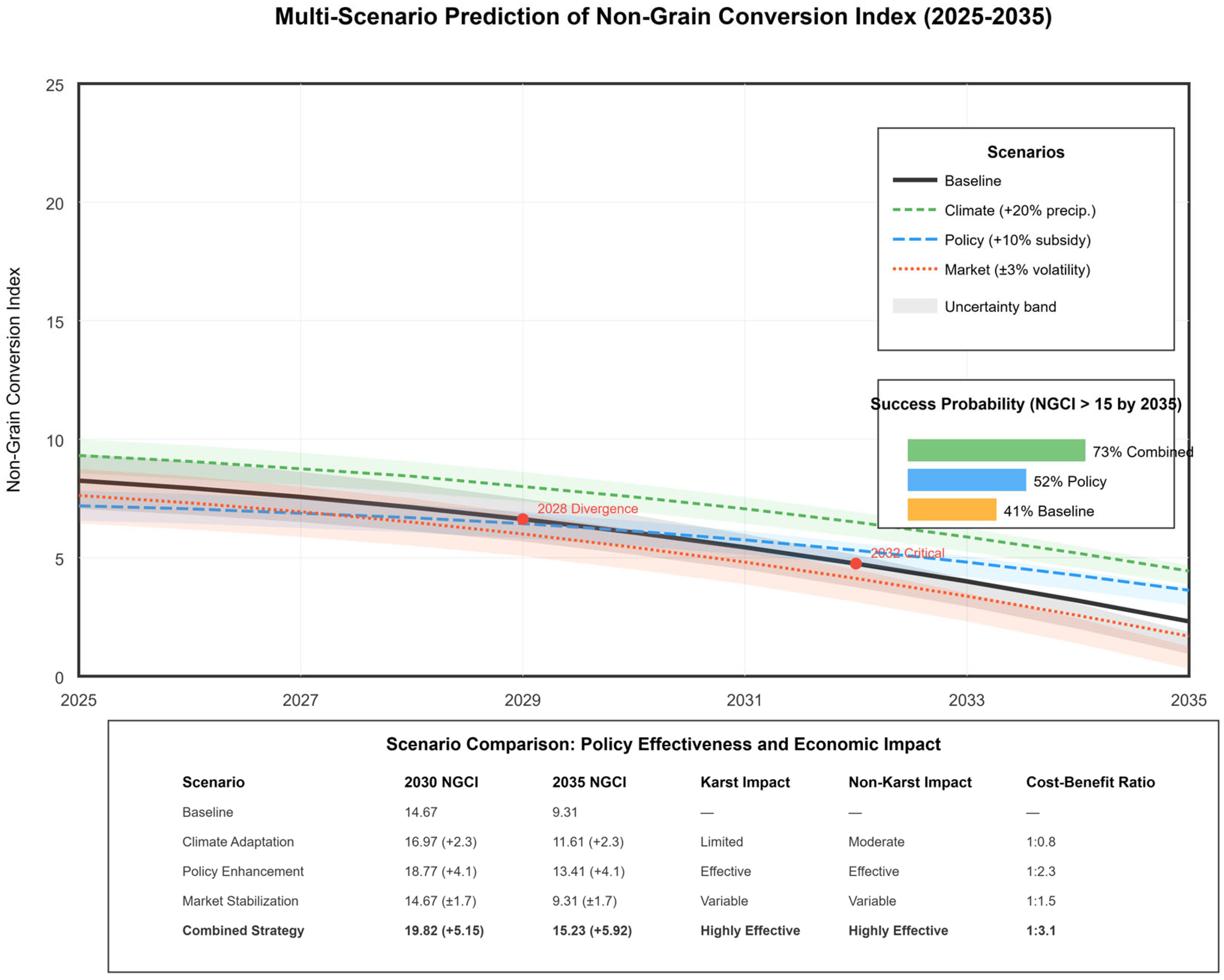
- The Dynamic Spatial-Temporal Clustering Model (DSTCM) achieved 92.51% pre-diction accuracy and identified NGCI = 10 as the critical threshold for irreversible agricultural degradation, with model projections indicating 89% of karst areas will cross this threshold by 2035 compared to 41% in non-karst regions.
- Karst terrain fundamentally alters agricultural land use decisions through geo-logical constraints (soil depth <30 cm, 40% lower water retention, 0.3ha average parcels), requiring specialized management strategies distinct from conventional agricultural regions to prevent irreversible degradation.
- Standard agricultural interventions demonstrate significantly reduced effective-ness in karst landscapes (3× higher implementation costs at 1340 CNY/hectare), while targeted karst-specific strategies incorporating soil conservation, water harvesting systems, and adapted crop varieties achieve 73% success probability in maintaining agricultural sustainability above critical thresholds.
Abstract
1. Introduction
2. Materials and Methods
2.1. Research Area and Data Introduction
2.1.1. Overview of the Research Area
2.1.2. Data Sources and Preprocessing
| Processing Stage | Method/Metric | Details | Result |
|---|---|---|---|
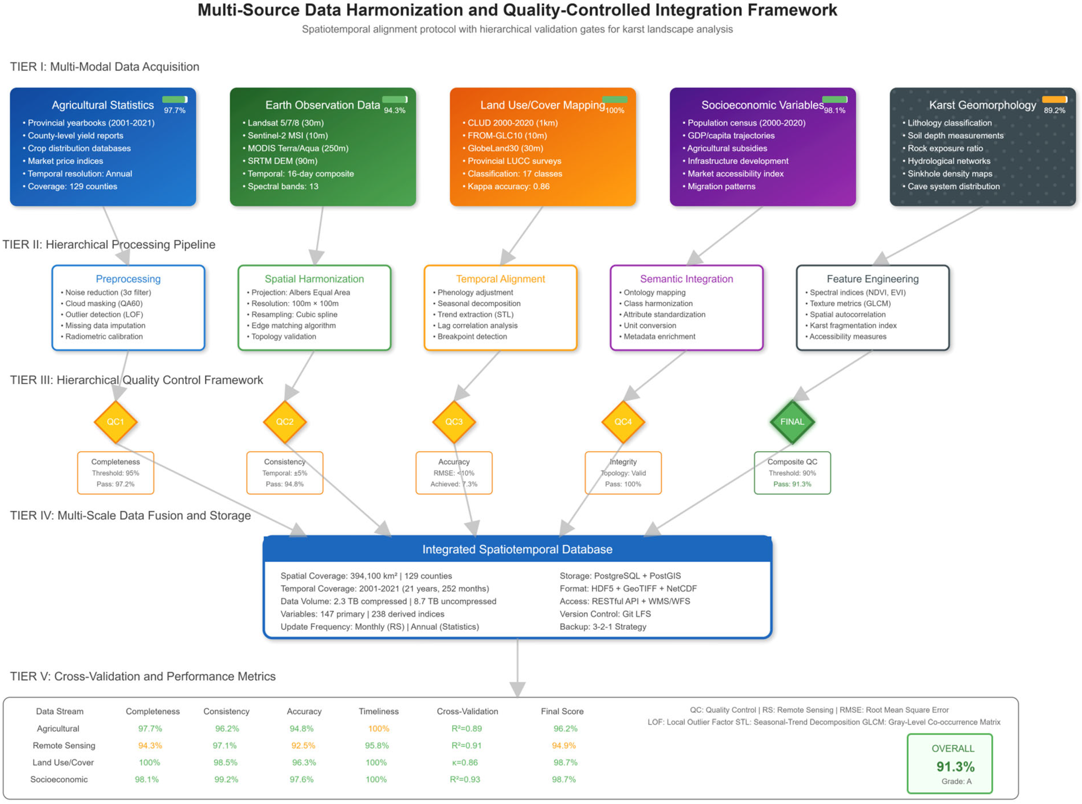
| Initial Data | Dataset Coverage | Planting area and production statistics | 129 counties (2001–2021) |
| Quality Control—Step A | Outlier Detection | Z-score method with threshold ± 3σ | 47 anomalous values identified |
| Quality Control—Step B | Verification | Cross-reference with Yunnan Statistical Yearbook | 31 transcription errors corrected |
| Quality Control—Step C | Missing Data Treatment | Weighted temporal interpolation | 2.3% gaps filled (RMSE = 0.034) |
| Quality Control—Step D | Validation | Correlation analysis with provincial totals | R2 = 0.97 achieved |
| Processing Step | Method | Specification | Result |
|---|---|---|---|
| (1) Original Resolution | Data Sources | Mixed resolution inputs | 30 m Landsat, 10 m Sentinel-2 |
| (2) Resampling | Standardization | Cubic convolution | Uniform 30 m grid |
| (3) Classification Accuracy | Accuracy Assessment | Overall accuracy measurement | 89.3%, Kappa = 0.86 |
| (4) Change Detection | Comparison Method | Post-classification comparison | 3 × 3 modal filter |
| (5) Validation | Field Verification | Stratified random points | 120 points (User’s accuracy = 91.2%) |
| Processing Step | Technique | Implementation | Performance |
|---|---|---|---|
| (1) Cloud Masking | Detection Algorithm | Fmask algorithm | Manual verification applied |
| (2) Temporal Composition | Pixel Selection | Median pixel value | Five least-cloudy images per year |
| (3) Atmospheric Correction | Correction Methods | Platform-specific processing | Sen2Cor (Sentinel-2), LEDAPS (Landsat) |
| (4) Radiometric Normalization | Normalization Method | Pseudo-invariant feature matching | Applied across all images |
| (5) NDVI Calculation | Compositing Method | Maximum value compositing | Growing season (April-October) |
| (6) Validation | Comparison Analysis | MODIS NDVI comparison | R2 = 0.83 |
| Integration Step | Process | Method Applied | Achievement |
|---|---|---|---|
| (1) Administrative Boundary Matching | Spatial Alignment | Boundary reconciliation | Ensured spatiotemporal consistency of administrative units |
| (2) Temporal Alignment | Time Series Harmonization | Linear interpolation | Quarterly to annual conversion |
| (3) Standardization | Data Normalization | Z-score normalization | Multi-scale integration achieved |
| (4) Validation | Accuracy Assessment | Residual analysis against census data | Mean Absolute Error = 3.2% |
2.2. Research Methods
2.2.1. Relevant Technologies Involved in the Research
Time Series Analysis Method
Spatial Agglomeration Analysis Method
CLUE-S Model
2.2.2. Research Process
3. Results
3.1. Time Series Analysis of Non-Grain Conversion Characteristics
3.2. Spatial Agglomeration Analysis
3.3. Analysis of Influencing Factors
3.4. Future Prediction Analysis
3.5. Scenario Analysis with Policy Implications
4. Discussions
4.1. Limitations and Future Research Priorities
4.2. Future Research Directions
5. Conclusions
Author Contributions
Funding
Data Availability Statement
Conflicts of Interest
References
- Chen, F.; Liu, J.N.; Chang, Y.Y.; Zhang, Q.; Yu, H.C.; Zhang, S.L. Spatial Pattern Differentiation and Driving Mechanism of Non-Grain Production of Cultivated Land in China. China Land Sci. 2021, 35, 11–27. [Google Scholar] [CrossRef]
- Chang, Y.Y.; Liu, J.N.; Ma, J.; Chen, F.; Yu, H.C. Spatial Pattern and Driving Factors of Non-Grain Production of Cultivated Land in Arid and Semi-Arid Areas. J. Agric. Resour. Environ. 2023, 40, 333–344. [Google Scholar] [CrossRef]
- Ren, G.; Song, G.; Wang, Q.; Sui, H. Impact of “Non-Grain” in Cultivated Land on Agricultural Development Resilience: A Case Study from the Major Grain-Producing Area of Northeast China. Appl. Sci. 2023, 13, 3814. [Google Scholar] [CrossRef]
- Perpiña Castillo, C.; Jacobs-Crisioni, C.; Diogo, V.; Lavalle, C. Modelling agricultural land abandonment in a fine spatial resolution multi-level land-use model: An application for the EU. Environ. Model. Softw. 2021, 136, 104946. [Google Scholar] [CrossRef] [PubMed]
- Du, G.M.; Li, N.N.; Zhang, N.; Wang, S.Y.; Liu, M.H. Analysis of Spatiotemporal Pattern of “Non-Grain Production” of Cultivated Land in China. J. Northeast Agric. Univ. Soc. Sci. Ed. 2022, 20, 17–27. [Google Scholar]
- Wang, P.C.; Zhang, L.G.; Lu, Y.L.; Chen, X.M.; Zhou, T.Y. Study on the Spatiotemporal Evolution and Influencing Factors of “Non-Grain Production” of Cultivated Land in Guangxi. China Agric. Resour. Reg. Plan. 2023, 44, 187–197. [Google Scholar]
- Wu, Y.; Yuan, C.; Liu, Z.; Wu, H.; Wei, X. Decoupling relationship between the non-grain production and intensification of cultivated land in China based on Tapio decoupling model. J. Clean. Prod. 2023, 424, 138800. [Google Scholar] [CrossRef]
- Yin, Q.; Wang, Y.; Yin, J. Analysis of Temporal and Spatial Changes of Cultivated Land in Karst Areas of Southwest Guangxi Based on Landscape Pattern Indices. Agric. Biotechnol. 2022, 11, 11–18. [Google Scholar]
- Panda, S.G.; Jena, R.K.; Rath, A.A.; Singh, K.N.; Tripathi, R.; Verma, H.K.H. Impact of institutional credit on agricultural productivity in India: A time series analysis. Indian J. Agric. Sci. 2020, 90, 412–417. [Google Scholar] [CrossRef]
- Zhang, L.L. Spatial Differentiation Characteristics and Zoning Remediation Strategies of “Non-Grain Production” of Cultivated Land in Longdong Loess Plateau Area—Taking Kongtong District, Gansu Province as an Example. Smart Agric. Guide 2023, 3, 59–62. [Google Scholar]
- Zhang, W.Z.; Cheng, Q.Y.; Cha, X.X. Study on the Influencing Factors of “Non-Grain Production” of Cultivated Land from the Perspective of Sustainable Development. Grain Sci. Technol. Econ. 2022, 47, 9–14. [Google Scholar] [CrossRef]
- Ji, Z.; Wang, X.; Li, L.; Guan, X.; Yu, L.; Xu, Y. The evolution of cultivated land utilization efficiency and its influencing factors in Nanyang Basin. J. Nat. Resour. 2021, 36, 688–701. [Google Scholar] [CrossRef]
- Chen, L.; Qiu, R.M.; Li, C. Spatiotemporal Evolution Characteristics and Driving Factors of Non-Grain Production of Cultivated Land in Chengdu Plain. Trop. Geogr. 2023, 43, 2406–2417. [Google Scholar] [CrossRef]
- Yang, B.W.; Liu, F.L.; Chen, H.M.; Zhang, Y.P.; Wang, K.L. Spatiotemporal Differentiation and Driving Force Analysis of Cultivated Land Non-Grain Production in Henan Province in the Past 20 Years. Shanghai Land Resour. 2024, 45, 72–85. [Google Scholar]
- Li, H.P.; Tian, D.R.; Tan, J.B. Spatiotemporal Pattern Evolution and Influencing Factors of Non-Agriculturalization of Cultivated Land in Yan’an City from 2000 to 2020. Bull. Soil Water Conserv. 2022, 42, 330–337. [Google Scholar] [CrossRef]
- Shao, Y.F. Study on the Spatial Pattern Differentiation, Causes and Countermeasures of “Non-Grain Production” of Cultivated Land in Henan Province. Hubei Agric. Sci. 2022, 61, 234–238. [Google Scholar] [CrossRef]
- Somerville, T.; Wetzel, J. Environmental hazards: The microgeography of land-use negative externalities. Real Estate Econ. 2022, 50, 468–497. [Google Scholar] [CrossRef]
- Fan, Y.; Li, X.; Jiang, S.; Liu, H. Construction and Evaluation of Ecological Security Patterns Using the PLUS Model and Circuit Theory: A Case Study of Liuzhou, China. Pol. J. Environ. Stud. 2025, 34, 1–24. [Google Scholar] [CrossRef]
- Li, L.; Pan, Y.; Zheng, R.; Liu, X. Understanding the spatiotemporal patterns of seasonal, annual, and consecutive farmland abandonment in China with time-series MODIS images during the period 2005–2019. Land Degrad. Dev. 2022, 33, 1608–1625. [Google Scholar] [CrossRef]
- Khan, S.A.; Vanselow, K.A.; Sass, O.; Samimi, C. Detecting abrupt change in land cover in the eastern Hindu Kush region using Landsat time series (1988–2020). J. Mt. Sci. 2022, 19, 1699–1716. [Google Scholar] [CrossRef]
- Wu, Y.L.; Zhang, P.; Yu, Y.Y.; Xie, R.Y. Research Progress and Prospect of “Non-Grain Production” of Cultivated Land in China from the Perspective of Food Security. China Land Sci. 2021, 35, 116–124. [Google Scholar] [CrossRef]
- Zhu, X.L.; Guo, Q.X. Scenario Simulation of Land Use Spatial Pattern Based on CLUE-S Model—Taking Xinfuqu of Xinzhou City as an Example. Jiangsu Agric. Sci. 2020, 48, 217–223. [Google Scholar]
- Tanjina Hasnat, G.N. Assessment of spatiotemporal distribution pattern of land surface temperature with incessant urban sprawl over Khulna and Rajshahi City Corporations. Environ. Chall. 2022, 9, 100644. [Google Scholar] [CrossRef]
- Fan, W.J.; Dai, X.A.; Xie, Y.R.; Gao, Y.F. Prediction and Analysis of Land Use Change in Sichuan Province in the Next 10 Years Using CLUE-S Model. Sci. Technol. Eng. 2022, 22, 2936–2942. [Google Scholar] [CrossRef]
- Atonya, S.; Olang, L.; Morara, L.; Nyandega, I.; Omuombo, C. Future Land-use Changes in the transboundary Sio-Malaba-Malakisi Basin of East Africa: Simulations using the CLUE-S model and Classified Satellite Land Cover Datasets. J. Sustain. Environ. Peace 2021, 4, 6–17. [Google Scholar]
- Mithiya, D.; Mandal, K.; Bandyopadhyay, S. Time Series Analysis and Forecasting of Rainfall for Agricultural Crops in India: An Application of Artificial Neural Network. Res. Agric. Eng. 2020, 12, 1–15. [Google Scholar] [CrossRef]
- Zhi, J.; Cao, X.; Liu, W.; Sun, Y.; Xu, D.; Da, C.; Jin, L.; Wang, J.; Zheng, Z.; Lai, S.; et al. Remote Sensing Monitoring and Spatial Pattern Analysis of Non-Grain Production of Cultivated Land in Anhui Province, China. Land 2023, 12, 1497. [Google Scholar] [CrossRef]
- Zhang, Z.; Zheng, L.; Yu, D. Non-Grain Production of Cultivated Land in Hilly and Mountainous Areas at the Village Scale: A Case Study in Le’an County, China. Land 2023, 12, 1562. [Google Scholar] [CrossRef]
- Hu, R.M.; Sun, Y.; Shi, X.L.; Wang, H.Y.; Li, J.M. Characteristics Identification of “Non-Grain Production” of Cultivated Land—Taking Dongxiang Autonomous County, Gansu Province as an Example. J. Xi’an Univ. Sci. Technol. 2022, 42, 453–461. [Google Scholar]
- Lamichhane, S.; Shakya, N.M. Land Use Land Cover (LULC) Change Projection in Kathmandu Valley using the CLUE-S Model. J. Adv. Coll. Eng. Manag. 2021, 6, 221–233. [Google Scholar] [CrossRef]
- Wang, J.; Zhang, D.; Nan, Y.; Liu, Z.; Qi, D. Spatial patterns of net primary productivity and its driving forces: A multi-scale analysis in the transnational area of the Tumen River. Front. Earth Sci. 2020, 14, 124–139. [Google Scholar] [CrossRef]
- Zhu, D.L. Economic Mechanism and Governance Path of “Non-Grain Production” of Cultivated Land. China Land 2021, 2021, 33–38. [Google Scholar]
- Prăvălie, R.; Patriche, C.; Tişcovschi, A.; Dumitraşcu, M.; Săvulescu, I.; Sîrodoev, I.; Bandoc, G. Recent spatio-temporal changes of land sensitivity to degradation in Romania due to climate change and human activities: An approach based on multiple environmental quality indicators. Ecol. Indic. 2020, 118, 106755. [Google Scholar] [CrossRef]
- Chen, S.; Wang, S.Z.; Lin, Y.B. Investigation and Reflection on Precise Implementation of Measures to Solve the Problem of “Non-Grain Production” of Cultivated Land. China Land 2022, 2022, 38–43. [Google Scholar]
- Sun, C.; Geng, N.; Wang, M. Regional Differences and Optimal Allocation of Cultivated Land Utilization Benefits Based on Improved TOPSIS Method: A Case Study of Guangxi. Asian Agric. Res. 2021, 13, 24–31. [Google Scholar]
- Youneszadeh, S.; Salajegheh, A.; Mesbahzadeh, T.; Tajrishi, M.; Khalighi Sigaroodi, S.; Taheri Shahraeini, H. Investigating the ability of Dyna-CLUE Model in Analyzing and Predicting Future Land Use Patterns in Simineh River Basin. Iran. J. Ecohydrol. 2021, 8, 73–87. [Google Scholar]
- Loukika, K.N.; Keesara, V.R.; Buri, E.S.; Sridhar, V. Future prediction of scenario based land use land cover (LU&LC) using DynaCLUE model for a river basin. Ecol. Inform. 2023, 77, 102223. [Google Scholar] [CrossRef]


| Region | Area (km2) | Karst Coverage (%) | Average Elevation (m) | Agricultural Justification |
|---|---|---|---|---|
| Central | 94,500 | 18% | 1890 | Economic center with urbanization pressure, the largest grain production base |
| Northwestern | 72,300 | 42% | 3200 | High-altitude karst with ecological protection priorities, unique alpine agriculture |
| Southwestern | 89,200 | 35% | 1650 | Tropical karst supporting rubber/tea, distinct from temperate crops elsewhere |
| Northeastern | 38,600 | 31% | 2100 | Traditional grain area with moderate karst influence |
| Southeastern | 45,800 | 38% | 1450 | Intensive karst landscape with the highest fragmentation, border trade influence |
| Dataset | Completeness (%) | Accuracy Metric | Validation Method | Result |
|---|---|---|---|---|
| Crop Yield | 97.7 | RMSE | Provincial totals correlation | R2 = 0.97 |
| Land Use | 100 | Kappa coefficient | Field points (n = 120) | 0.86 |
| Remote Sensing | 94.3 | RMSE (NDVI) | MODIS comparison | 0.083 |
| Demographic | 98.1 | MAE | Census validation | 3.20% |
| Model Type | Purpose | Mathematical Formula | Parameters |
|---|---|---|---|
| (1) ARMA | Captures autoregressive and moving average features | X11 = μ + Σᵢ=1ᵖ φᵢXₜ−ᵢ + Σⱼ=1ᵍ θⱼεₜ−j + εₜ |
|
| (2) ARIMA | Eliminates trend through differencing for data stability | X12 = μ + Σᵢ₌1ᵖ φᵢXₜ−ᵢ + Σⱼ₌1ᵍ θⱼεₜ−ⱼ + εₜ + Σₖ₌1ᵈ Δᵈ Xₜ−ₖ |
|
| (3) SARIMA | Incorporates seasonal patterns into the model | X13 = μ + Σᵢ₌1ᵖ φᵢXₜ−ᵢ + Σⱼ₌1ᵍ θⱼεₜ−ⱼ + Σₛ₌1ᴾ Φₛ Xₜ−ₛₛ + Σₒ₌1ᵠ Θₒ εₜ−ₒₛ + εₜ |
|
| Step | ARMA | ARIMA | SARIMA |
|---|---|---|---|
| Primary Function | Baseline time series modeling | Trend elimination and stabilization | Seasonal pattern integration |
| Calculation Order |
|
|
|
| Data Requirements | Stationary time series | Non-stationary time series | Time series with seasonal patterns |
| Model Complexity | Basic | Intermediate | Advanced |
| Component | Symbol | Description | Specification |
|---|---|---|---|
| Formula | CPIt | ∑(i = 1 to n) (PCi · Yi · Ri)/∑(i = 1 to n) (PCi · Yi · Ri)_baseline | Equation (5) |
| Number of crop types | n | Total crop categories tracked | Food crops: rice, wheat; Non-food crops: vegetables, fruits, rubber, tea |
| Market price | PCi | Market price of cropi | Current year values |
| Crop yield | Yi | Yield of cropi | Production per unit area |
| Planting area proportion | Ri | Planting area/total cultivated land area | Percentage of total cultivated land |
| Baseline reference | baseline | Reference year for comparison | Year 2001 data |
| Component | Symbol | Description | Specification |
|---|---|---|---|
| Formula | LUIt | ∑(j = 1 to m) (LUj,t · Wj)/∑(j = 1 to m) (LUj,baseline · Wj) | Equation (6) |
| Land use types | m | Number of land categories | Cultivated land, forest land, grassland |
| Time indicator | t | Current time period | Annual measurement |
| Land area | LUj,t | Area of land type j at time t | Measured in hectares |
| Land type weight | Wj | Weight based on non-grainization contribution | Determined by land type’s role in conversion process |
| Component | Symbol | Description | Specification |
|---|---|---|---|
| Formula | RSIt | (NDVIt + LCIt + VFCt)/(NDVIbaseline + LCIbaseline + VFCbaseline) | Equation (7) |
| Vegetation index | NDVIt | Normalized difference vegetation index | Reflects vegetation cover change |
| Land cover change | LCIt | Land cover change index | Based on proportion of cultivated land vs non-food purposes |
| Vegetation coverage | VFCt | Vegetation fractional coverage | Percentage of vegetation cover |
| Component | Symbol | Description | Specification |
|---|---|---|---|
| Formula | PSIt | (URt · POPt + GDPt · ARt)/(URbaseline · POPbaseline + GDPbaseline · ARbaseline) | Equation (8) |
| Urbanization rate | URt | Degree of rural-urban population transfer | Percentage of urban population |
| Population density | POPt | Population per unit area | Persons per square kilometer |
| Regional GDP | GDPt | Gross regional product | Economic output measure |
| Agricultural employment | ARt | Proportion employed in agriculture | Percentage of workforce in agricultural sector |
| Symbol | Definition | Units | Range |
|---|---|---|---|
| NGCI(t) | Non-Grain Conversion Index at time t | Dimensionless | [0, 100] |
| α, β, γ, δ | Component weights | Dimensionless | [0, 1] |
| CPI(t) | Crop Pattern Index | Dimensionless | [0, 100] |
| LUI(t) | Land Use Index | Dimensionless | [0, 100] |
| RSI(t) | Remote Sensing Index | Dimensionless | [0, 100] |
| PSI(t) | Population-Socioeconomic Index | Dimensionless | [0, 100] |
| N | Number of spatial units | Count | 129 (counties) |
| I | Moran’s I statistic | Dimensionless | [−1, 1] |
| C | Geary’s C coefficient | Dimensionless | [0, ∞) |
| Step | Component | Details |
|---|---|---|
| Step 1: Stationarity Testing | Augmented Dickey-Fuller Test | Ho: series has unit root |
| Original Series Results | Non-stationary (p = 0.31) | |
| After First Differencing | Stationary (p < 0.01) | |
| Step 2: Model Identification | ACF/PACF Analysis | Reveals AR(2) and MA(1) components |
| Seasonal Pattern | Detected at lag4(annual crop cycle) | |
| Step 3: Parameter Estimation ARIMA(2,1,1) Model | Model Equation | (Equation 9) |
| Standard Errors | SE(ψ1) = 0.09 SE(ψ2) = 0.08 SE(∅3) = 0.07 | |
| Model Type | ARIMA(2,1.1) | |
| Step 4: Diagnostic Checking | Ljung-Box Test | Q(12) = 8.73, p = 0.43 (white noise residuals) |
| Residual Normality | Shapiro-Wilk p = 0.21 | |
| Heteroscedasticity Test | Breusch-Pagan p = 0.38 (no heteroscedasticity) |
| From/To | Grain | Non-Grain | Non-Agricultural |
|---|---|---|---|
| Grain | 0.83 | 0.14 | 0.03 |
| Non-grain | 0.08 | 0.87 | 0.05 |
| Non-agricultural | 0.01 | 0.02 | 0.97 |
| Method | Key Build Processes | Parameter Indicators |
|---|---|---|
| Time series analysis | The “ts” package in R language was used to load land use data, and time series analysis was carried out to calculate the trend and seasonal changes in non-grain cultivated land. | After loading the data, the time series was first smoothed using a 3-year moving average. The periodicity and trend of the time series were determined and verified by ADF (Augmented Dickey–Fuller) test or periodicity analysis method. |
| Spatial agglomeration analysis | ArcGIS software was used to load the remote sensing image data, and the spatial clustering analysis was carried out to identify the hot and cold spots of non-grain cultivated land. | After the data is loaded, the ordinary Kriging interpolation method is used to fill the data gaps, and the interpolation parameters are set to default values. A spatial distance of 500 m and a neighborhood parameter of 5 were determined for the cluster analysis. Hopkins statistic was used to evaluate the stability and effectiveness of clustering, and the effects of different clustering methods were compared. |
| Multiple linear regression model | The “statsmodels” package in Python3.13.5 was used to load the cleaned crop yield data and demographic data, and a multiple linear regression model was established to analyze the factors affecting the non-grain of cultivated land. | Before the establishment of the model, data preprocessing is carried out to remove outliers and missing values. Stepwise regression was used to select the best predictor variables, and the significance level was set at 0.05. R2 value, adjusted R 2 value and residual analysis were used to evaluate the fitting degree and prediction effect of the model [32]. |
| CLUE-S model | CLUE-S model software was used to load land use and demographic data, set model parameters, simulate the development trend of non-grain cultivated land in the future, and put forward preventive strategies. | Before setting the model parameters, the sensitivity analysis is carried out to determine the parameter range. The genetic algorithm was used to optimize the model parameters, and the number of iterations was set to 1000. Initial state setting sets the initial proportion of cultivated land, forest land and construction land to 30%, 50% and 20%. In the factor weight setting, the weight of cultivated land protection policy impact factor can be set to 0.7, and the weight of economic development factor can be set to 0.5. The calculation of probability transition matrix is based on Markov process theory to calculate the transition probability between different land use types. Kappa coefficient and model accuracy index are used in the verification process, and genetic algorithm is used to find the parameter combination that maximizes the model accuracy index in the optimization process. Kappa coefficient and model accuracy index were used to evaluate the predictive ability and accuracy of the model [33,34,35]. |
| Name of the Factor | Classification Criteria | Factor Interpretation |
|---|---|---|
| Soil fertility | Suitability of land use | Soil fertility is directly related to the suitability of land, and high-fertility land may be more easily used for non-food crop cultivation. |
| Slope | Suitability of land use | Flatter land is more accessible to agricultural activities and may be more suitable for non-food cropland use. |
| Average annual precipitation | Climatic suitability | Precipitation has a direct impact on the growth of different crops and is closely related to climate suitability. |
| Average annual temperature | Climatic suitability | Temperature is a key factor for crop growth, and different crops have different requirements for temperature. |
| Main crop types | Crop suitability | Different crops have different adaptability to land use patterns, which may lead to different degrees of non-food production. |
| Utilization rate of cultivated land | Degree of cultivated land use | The intensity of cultivated land use reflects whether the land is fully used, which may be related to the degree of non-grain production. |
| GDP (Gross Domestic Product) level | The economic base | Regional economic level may affect farmers’ land use decisions, and thus affect the degree of non-grain production. |
| Agricultural subsidy policy | The economic base | Different agricultural subsidy policies may affect farmers’ crop selection and cultivated land use, which is related to non-food production. |
| Urbanization rate | The economic base | The process of urbanization may promote the transformation of agricultural land to other uses, which is closely related to non-grain production. |
| Level of science and technology | The economic base | Advanced agricultural technology may improve agricultural productivity, change the way of land use, and affect the trend of non-food production. |
| Ecological environment health | The economic base | The state of the ecological environment may affect the sustainable use of land, thus affecting the degree of non-food production. |
| Prices of agricultural products | The economic base | Fluctuations in the prices of agricultural products may affect farmers’ choice of crops and the use of arable land, and have an impact on non-grain production. |
| Cost of agricultural production | The economic base | The change in agricultural production cost will affect the economic decision-making of farmers, which may lead to the adjustment of cultivated land use and the emergence of a non-grain phenomenon. |
| Livelihood of farmers | The economic base | The livelihood of farmers is directly related to the way they use the land, and economic pressure may prompt farmers to choose non-food crops with more economic benefits. |
| Land ownership system | Social system | Different land ownership systems may affect the way of land use and the decision-making behavior of farmers, thus affecting the degree of non-grain cultivated land. |
| Policy support | Policy and system | The government’s support and policy guidance for agricultural development may directly affect farmers’ planting choices and cultivated land use, and then affect the development of non-grain crops. |
| Selection Criterion | Methodology | Implementation Details | Outcome |
|---|---|---|---|
| Theoretical Foundation | Literature-based selection | Factors identified from established agricultural land use change research combined with Yunnan Province’s specific agricultural development context | Initial factor pool established based on empirical evidence |
| Multicollinearity Testing | Variance Inflation Factor (VIF) analysis | Variables with VIF > 10 examined for removal or combination. Example: GDP level showed correlation with agricultural production costs (r = 0.68) and agricultural product prices (r = 0.72) | GDP retained as composite economic indicator with adjusted weights |
| Data Availability and Quality | Temporal coverage assessment | Complete data coverage requirement for 2001–2021 period with verification of source reliability | Only factors meeting full temporal coverage included |
| Geographical Factors Consideration | Indirect incorporation strategy | Topographical factors (DEM, distance to roads, proximity to rivers) incorporated through slope variable and spatial analysis components. Stable geographical features over 2001–2021 period would not significantly affect temporal dynamics | Influence captured through spatial heterogeneity patterns in autocorrelation analysis |
| Regional Relevance | Proxy variable representation | Yunnan-specific factors (ethnic minority population distribution, cross-border trade intensity) represented through proxy variables due to data limitations | Farmer livelihood conditions and agricultural product prices serve as proxy indicators |
| Dataset Name | Evaluation Benchmark | Evaluation Scale | Measure Basis 1 | Weight by 1 | Measure Basis 2 | Basis 2 Weight |
|---|---|---|---|---|---|---|
| Crop yield data | Administrative Unit | Macro scale | Planting structure | 0.55 | Yield factor | 0.45 |
| Land use data | Administrative Unit | Macro scale | Land type | 0.40 | Utilization | 0.60 |
| Remote sensing image data | Spatial unit (pixel) | Micro scale | Coverage | 0.70 | Change trend | 0.30 |
| Demographic data | Administrative Unit | Macro scale | Population density | 0.60 | Urbanization trend | 0.40 |
| Evaluation Indicators | Selection Basis | Value Range | Evaluation Criteria |
|---|---|---|---|
| Moran’s I mean | Global Spatial Autocorrelation for Measuring Non-gratification | [−1, 1] | 0 indicates a random distribution, 1 indicates a perfect positive correlation, and −1 indicates a perfect negative correlation. |
| NDVI (Normalized Difference Vegetation Index) average | Reflect the status of vegetation in non-grain area | [−1, 1] | 0 means no vegetation and 1 means dense vegetation. |
| LISA (Local Indicators of Spatial Association) mean | Identify local areas of spatial agglomeration | [−1, 1] | 1 indicates a high degree of positive spatial autocorrelation, and −1 indicates a high degree of negative spatial autocorrelation. |
| Geary’s C mean | Characterizing the spatial distribution of non-grain in the region | [0, ∞) | 0 means complete spatial autocorrelation, and ∞ means complete spatial heterocorrelation. |
| Spatial diffusion average | Reflect the spatial transmission trend of non-food | [0, 1] | 0 means no diffusion and 1 means complete diffusion. |
| Z-score mean of the Getis-Ord GI * statistic | Emphasize the spatial clustering significance of high or low values | No fixed range | Positive values indicate clustering of high values, negative values indicate clustering of low values, and 0 indicates a random distribution. |
| Phase | Period | NGCI Values & Changes | Regional Differences | Statistical Significance | Additional Observations |
|---|---|---|---|---|---|
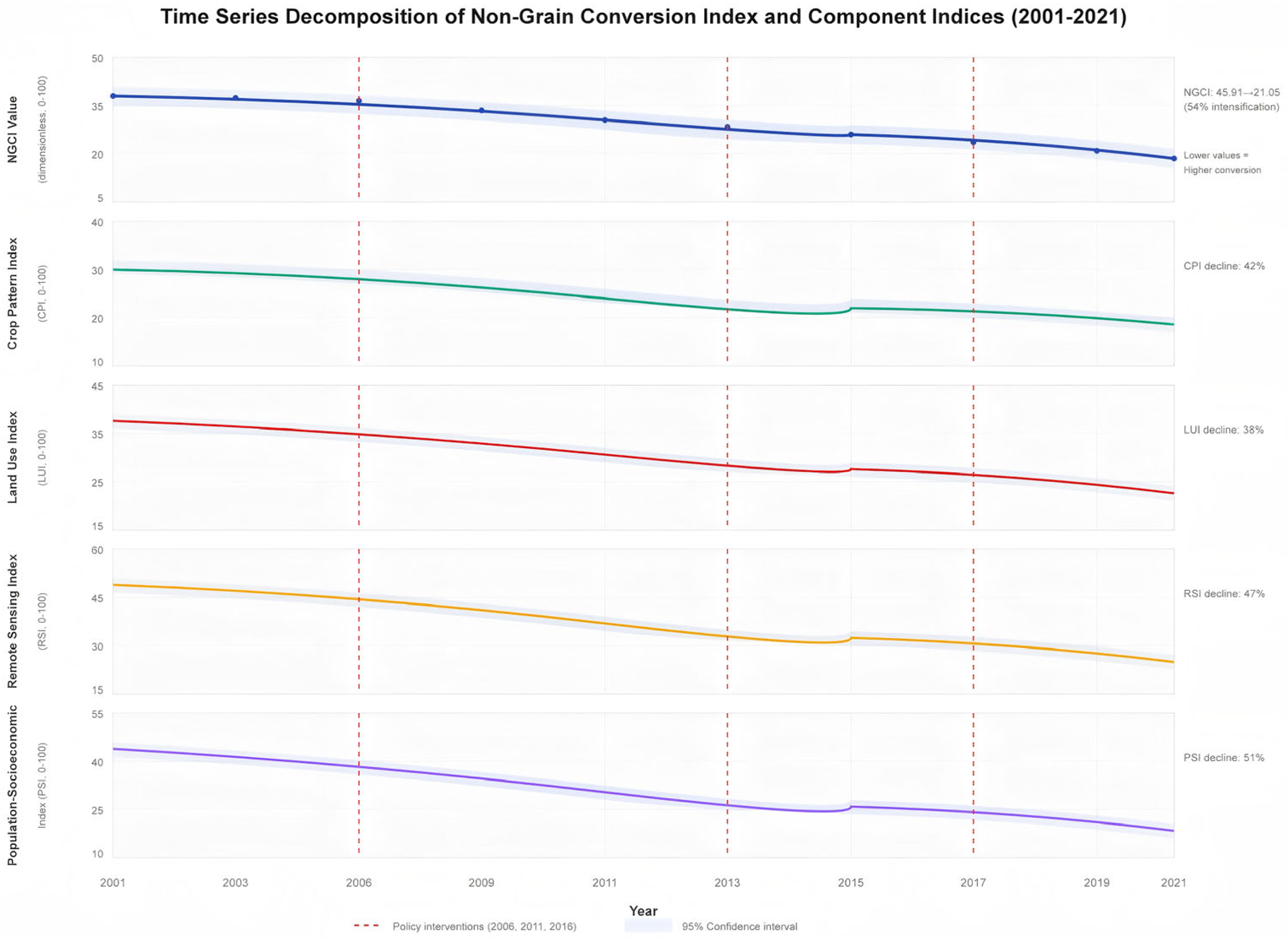
| Phase 1: Initial Shock Period | 2001–2006 | NGCI maintained > 35 (limited conversion) | Karst areas: NGCI = 38.2 ± 2.1 Non-karst areas: NGCI = 41.3 ± 1.8 | Difference statistically significant (t = 3.21, p = 0.002) | - |
| Phase 2: Transition Period | 2007–2015 | NGCI declined from 36.26 to 33.04 (9% intensification) | - | - | (1) Introduction of ecological compensation policies in karst regions (2) Crop yield index recovery from 21.75 to 28.81 indicates adaptation |
| Phase 3: Acceleration Period | 2016–2021 | NGCI dropped from 30.56 to 19.05 (38%intensification in 6 years) | Karst areas reached NGCI = 16.2, approaching critical threshold | Structural break test confirms 2016 changepoint (Chow test F =14.3, p < 0.001) | - |
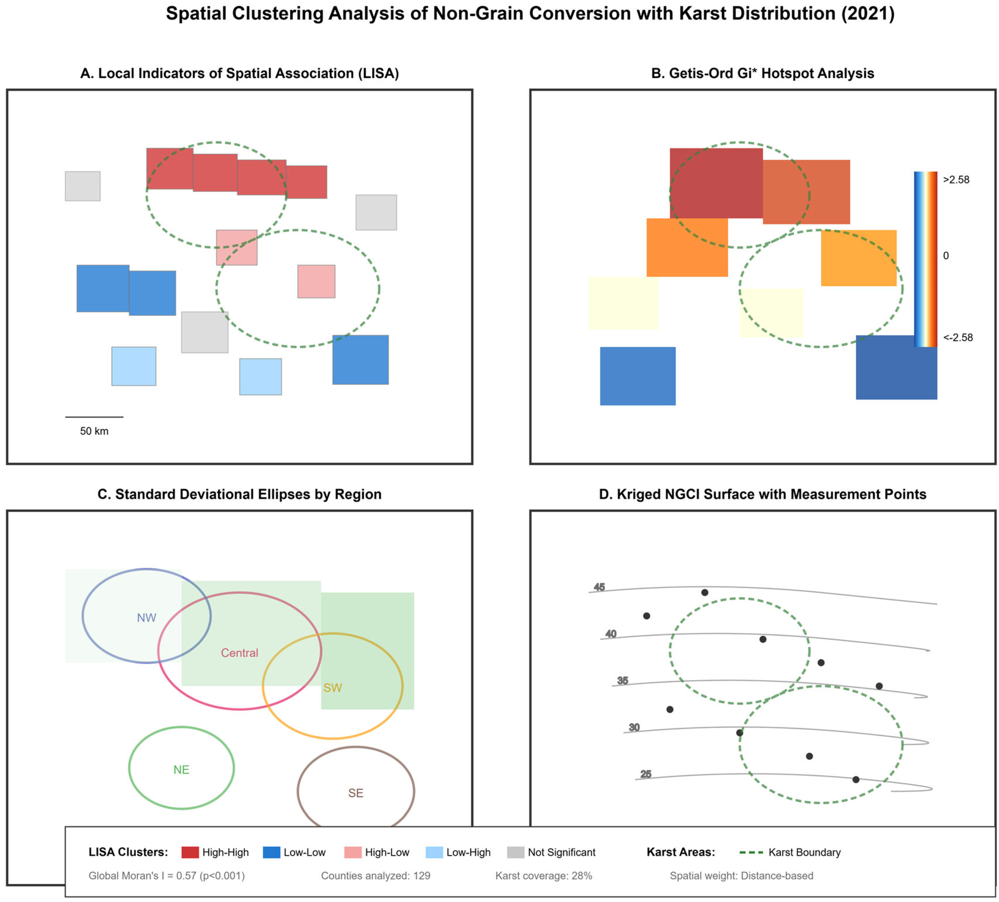
| Karst Coverage | Moran’s I | Geary’s C | Geary’s C | Counties (n) |
|---|---|---|---|---|
| <10% (Low) | 0.41 ± 0.08 | 1.48 ± 0.12 | 1.23 ± 0.31 | 28 |
| 10–30% (Moderate) | 0.52 ± 0.06 | 1.41 ± 0.09 | 1.89 ± 0.28 | 45 |
| 30–50% (High) | 0.68 ± 0.05 | 1.32 ± 0.07 | 2.34 ± 0.25 | 38 |
| >50% (Intensive) | 0.73 ± 0.04 | 1.28 ± 0.06 | 2.67 ± 0.22 | 18 |
| Factor | Main Effect | Karst Interaction | Combined Effect |
|---|---|---|---|
| t-value (p) | t-value (p) | Marginal Effect | |
| Soil fertility | 2.35 (0.027) | 3.12 (0.003) | 0.43 in karst, 0.21 elsewhere |
| Main crop types | 3.12 (0.047) | 2.87 (0.006) | Stronger in karst |
| GDP level | 2.88 (0.012) | 1.23 (0.224) | No karst interaction |
| Technology level | 2.67 (0.019) | −2.31 (0.024) | Weaker in karst |
| Slope | −0.92 (0.376) | 4.56 (0.000) | Critical in karst |
| Water availability | 1.78 (0.095) | 3.89 (0.000) | Limiting in karst |
| Factor | Central Yunnan (t-Value, p-Value) | Northwest Yunnan (t, p) | Southwest Yunnan (t Value, p Value) | Northeast Yunnan (t Value, p Value) | Southeast Yunnan (t Value, p Value) |
|---|---|---|---|---|---|
| Soil fertility | 2.10, 0.035 | 2.01, 0.042 | 2.25, 0.031 | 2.18, 0.038 | 1.95, 0.047 |
| Slope | −0.85, 0.401 | −0.97, 0.367 | −0.78, 0.445 | −0.92, 0.388 | −0.88, 0.412 |
| Average annual precipitation | 1.68, 0.096 | 1.75, 0.088 | 1.82, 0.081 | 1.71, 0.101 | 1.65, 0.105 |
| Average annual temperature | −1.35, 0.178 | −1.42, 0.163 | −1.30, 0.192 | −1.38, 0.171 | −1.32, 0.185 |
| Main crop types | 2.95, 0.015 | 2.82, 0.019 | 3.08, 0.012 | 2.89, 0.017 | 2.97, 0.014 |
| Utilization rate of cultivated land | −0.55, 0.589 | −0.60, 0.564 | −0.52, 0.609 | 0.58, 0.576 | −0.57, 0.581 |
| GDP level | 2.75, 0.018 | 2.89, 0.015 | 2.68, 0.021 | 2.80, 0.017 | 2.72, 0.020 |
| Agricultural subsidy policy | 1.88, 0.065 | 1.94, 0.057 | 1.82, 0.071 | 1.90, 0.062 | 1.86, 0.068 |
| Urbanization rate | −0.34, 0.738 | −0.38, 0.712 | −0.32, 0.752 | −0.36, 0.729 | −0.35, 0.734 |
| Level of science and technology | 2.57, 0.022 | 2.49, 0.027 | 2.62, 0.019 | 2.54, 0.024 | 2.59, 0.021 |
| Ecological environment health | −1.02, 0.309 | −1.08, 0.284 | −0.98, 0.321 | −1.05, 0.298 | −1.00, 0.312 |
| Prices of agricultural products | 1.24, 0.034 | 1.27, 0.037 | 1.21, 0.031 | 1.25, 0.035 | 1.29, 0.038 |
| Cost of agricultural production | −0.56, 0.287 | −0.58, 0.292 | −0.54, 0.281 | −0.57, 0.289 | −0.55, 0.284 |
| Livelihood of farmers | 2.45, 0.015 | 2.42, 0.014 | 2.48, 0.017 | 2.43, 0.016 | 2.50, 0.018 |
| Land ownership system | −1.24, 0.129 | −1.26, 0.132 | −1.22, 0.126 | −1.25, 0.131 | −1.23, 0.127 |
| Policy support | 0.78, 0.455 | 0.80, 0.460 | 0.76, 0.448 | 0.79, 0.457 | 0.77, 0.452 |
| Model overall significance | 4.45, 0.002 | 4.52, 0.001 | 4.40, 0.003 | 4.48, 0.002 | 4.43, 0.002 |
| Year | NGCI Prediction | 95% CI | Karst Areas | Non-Karst |
|---|---|---|---|---|
| 2025 | 20.08 | [18.34, 21.82] | 17.23 | 22.45 |
| 2030 | 14.67 | [12.11, 17.23] | 11.34 | 17.89 |
| 2035 | 9.31 | [6.23, 12.39] | 5.67 | 12.78 |
| Scenario | Parameter Change | Karst Impact | Non-Karst Impact | Policy Effectiveness |
|---|---|---|---|---|
| Climate Adaptation | +20% precipitation | NGCI + 2.3 | NGCI + 0.8 | Limited in karst due to drainage |
| Subsidy Enhancement | +10% grain subsidies | NGCI + 4.1 | NGCI + 3.2 | Effective if targeted to karst |
| Market Stabilization | ±3% price volatility | NGCI ± 1.7 | NGCI ± 2.1 | Similar effectiveness |
| Technology Package | Precision agriculture | NGCI + 1.2 | NGCI + 3.8 | Barriers in fragmented karst |
| Ecological Restoration | 20% land retirement | NGCI − 8.3 | NGCI − 3.1 | Major impact in degraded karst |
Disclaimer/Publisher’s Note: The statements, opinions and data contained in all publications are solely those of the individual author(s) and contributor(s) and not of MDPI and/or the editor(s). MDPI and/or the editor(s) disclaim responsibility for any injury to people or property resulting from any ideas, methods, instructions or products referred to in the content. |
© 2025 by the authors. Licensee MDPI, Basel, Switzerland. This article is an open access article distributed under the terms and conditions of the Creative Commons Attribution (CC BY) license (https://creativecommons.org/licenses/by/4.0/).
Share and Cite
Ma, X.; Tang, B.; He, F.; Huang, L.; Zhang, Z.; Cui, D. Extraction and Prediction of Spatiotemporal Pattern Characteristics of Farmland Non-Grain Conversion in Yunnan Province Based on Multi-Source Data. Remote Sens. 2025, 17, 3295. https://doi.org/10.3390/rs17193295
Ma X, Tang B, He F, Huang L, Zhang Z, Cui D. Extraction and Prediction of Spatiotemporal Pattern Characteristics of Farmland Non-Grain Conversion in Yunnan Province Based on Multi-Source Data. Remote Sensing. 2025; 17(19):3295. https://doi.org/10.3390/rs17193295
Chicago/Turabian StyleMa, Xianguang, Bohui Tang, Feng He, Liang Huang, Zhen Zhang, and Dongguang Cui. 2025. "Extraction and Prediction of Spatiotemporal Pattern Characteristics of Farmland Non-Grain Conversion in Yunnan Province Based on Multi-Source Data" Remote Sensing 17, no. 19: 3295. https://doi.org/10.3390/rs17193295
APA StyleMa, X., Tang, B., He, F., Huang, L., Zhang, Z., & Cui, D. (2025). Extraction and Prediction of Spatiotemporal Pattern Characteristics of Farmland Non-Grain Conversion in Yunnan Province Based on Multi-Source Data. Remote Sensing, 17(19), 3295. https://doi.org/10.3390/rs17193295


