Spatiotemporal Interactive Learning for Cloud Removal Based on Multi-Temporal SAR–Optical Images

Abstract

Optical remote sensing images suffer from information loss due to cloud interference, while Synthetic Aperture Radar (SAR), capable of all-weather and day–night imaging capabilities, provides crucial auxiliary data for cloud removal and reconstruction. However, existing cloud removal methods face the following key challenges: insufficient utilization of spatiotemporal information in multi-temporal data, and fusion challenges arising from fundamentally different imaging mechanisms between optical and SAR images. To address these challenges, a spatiotemporal feature interaction-based cloud removal method is proposed to effectively fuse SAR and optical images. Built upon a conditional generative adversarial network framework, the method incorporates three key modules: a multi-temporal spatiotemporal feature joint extraction module, a spatiotemporal information interaction module, and a spatiotemporal discriminator module. These components jointly establish a many-to-many spatiotemporal interactive learning network, which separately extracts and fuses spatiotemporal features from multi-temporal SAR–optical image pairs to generate temporally consistent, cloud-free image sequences. Experiments on both simulated and real datasets demonstrate the superior performance of the proposed method.

1. Introduction

Optical remote sensing imagery has emerged as a pivotal technical means for acquiring surface information. However, constrained by its passive imaging mechanisms, optical remote sensing imagery is susceptible to cloud contamination. Statistical data reveal that approximately 67% [1] of the Earth’s surface is persistently obscured by clouds, substantially diminishing the practical value of remote sensing imagery for critical downstream applications including fusion [2], unmixing [3], and target detection [4]. This persistent challenge underscores the urgent need to develop robust and high-quality cloud removal solutions as an important research topic.

Currently, numerous methods have been proposed for cloud removal in optical remote sensing images, including the temporal-based cloud removal methods, spatial-based methods, spectral-based methods, and temporal–spatial–spectral joint-based methods [5]. Temporal-based methods leverage the periodic sampling characteristics of remote sensing satellites, employing multi-temporal imagery of the same geographic area to reconstruct cloud-contaminated regions. Representative approaches include replacement-based methods [6,7,8,9,10], filtering techniques [11], and learning-based algorithms [12,13]. However, these methods are all based on the assumption that no significant surface changes occur between the temporal images. These methods fail when either significant surface changes occur within a short period or cloud-free reference images from adjacent time periods are lacking. The scarcity of qualified remote sensing data hinders the development of temporal cloud removal methods. Spatial-based methods originate from natural image inpainting theory, utilizing information from cloud-free regions to reconstruct cloud-contaminated regions. Representative methods include interpolation-based approaches [14,15], diffusion propagation techniques [16,17], variational optimization methods [18], and exemplar-based algorithms [8]. In recent years, learning-based methods, with Generative Adversarial Networks (GANs) [19] as a prime example, have been widely adopted in cloud removal applications. Although these direct restoration techniques require no auxiliary data, their practical effectiveness is limited to small-scale cloud-contaminated areas due to their strict dependence on similar contextual structures. When dealing with continuous large-area cloud contamination, the reliability of reconstruction results decreases significantly. The inherent spectral redundancy in remote sensing images enables the reconstruction of missing data in specific spectral bands. Spectral-based methods leverage bands with greater cloud-penetration capability to acquire information and reconstruct spectral data in cloud-contaminated areas based on the premise of strong inter-band correlations. Representative methods include polynomial fitting [11,20,21] and GAN models [22,23]. While demonstrating satisfactory performance under thin cloud conditions, these methods face significant limitations when all image bands are obscured by opaque, thick clouds. The cloud removal methods discussed above demonstrate distinct advantages in certain scenarios, yet they typically reconstruct missing data using only one or two types of information, leading to limited information utilization. To overcome this limitation, temporal–spatial–spectral joint-based methods achieve reconstruction of cloud-contaminated regions through synchronous utilization of correlated information across spatial, spectral, and temporal dimensions. Ng et al. [24] proposed an adaptive weighted tensor completion algorithm that optimizes weight allocation across different dimensions. Ji et al. [25] constructed multi-temporal remote sensing images as fourth-order tensors, achieving high-fidelity reconstruction of cloud-contaminated areas through tensor low-rank decomposition combined with non-local similarity constraints. Lin et al. [26] proposed the Robust Thick Cloud Removal model, which effectively handles thick cloud occlusion by coupling tensor decomposition. Liu et al. [27] developed a low-rank tensor completion algorithm termed high accuracy low rank tensor completion for missing value estimation. He et al. [28] proposed the total variation-regularized tensor ring completion model by integrating total variation with low-rank tensor ring regularization. However, these methods generally rely on manually designed prior knowledge, making it difficult to fully capture the details and textures of multi-temporal remote sensing images, thereby limiting their performance.

Synthetic Aperture Radar (SAR) demonstrates unique advantages in cloud removal applications due to its all-weather and day–night imaging capabilities [29]. In recent years, cloud removal methods utilizing SAR images have emerged as a research hotspot in this field. These approaches can be broadly categorized into single SAR image-based cloud removal methods and SAR–optical joint cloud removal methods. Single SAR image-based methods typically employ deep learning frameworks to directly map SAR images to optical images. For instance, Bermudez et al. [30] utilized GANs to transform SAR images into cloud-free optical images for cloud removal. However, due to the significant modality gap between optical and SAR images, the reliability of cloud removal based solely on a single SAR image remains limited.

The joint cloud removal approach synergistically utilizes both SAR and optical imagery information for effective cloud removal. This methodology can be categorized into single-temporal and multi-temporal approaches. Single-temporal methods utilize SAR and optical images acquired at the same time. For example, Darbaghshahi et al. [31] transformed SAR images into optical modality for fusion with cloud-contaminated images; however, the effectiveness was constrained by SAR image quality. Xu et al. [32] enhanced cloud removal performance by integrating global and local features from SAR data. Huang et al. [33] employed a sparse representation-based method to combine MODIS low-resolution optical images with SAR data, effectively restoring cloud-contaminated regions. Grohnfeldt et al. [34] achieved remarkable results using conditional GANs to reconstruct cloud-contaminated optical images by exploiting SAR–optical complementarity. Meraner et al. [35] implemented residual networks to generate cloud-free imagery through SAR–optical fusion. Regarding multi-temporal approaches, He et al. [36] investigated the feasibility of generating optical imagery using both single SAR images and multi-temporal SAR–optical image pairs. Bermudez et al. [37] reconstructed missing regions in optical images using conditional GANs (cGANs) with multi-modal, multi-temporal SAR and optical data. Xia et al. [38] further improved the performance of the network by integrating temporal SAR constraints. However, current SAR-assisted methods still face two major limitations: inadequate utilization of spatiotemporal information inherent in multi-temporal SAR and optical data, and significant challenges in achieving effective optical-SAR image fusion.

To address these challenges, we propose an interesting “many-to-many” cloud removal framework for multi-temporal SAR and optical image fusion, based on spatiotemporal information interaction. This method establishes a spatiotemporal interactive learning network that constructs a mapping from cloud-contaminated multi-temporal SAR–optical image pairs to cloud-free optical image sequences, thereby achieving comprehensive utilization of remote sensing data information. The main contributions of this work are as follows:

• We proposed a spatiotemporal interactive learning network for cloud removal based on multi-temporal SAR and optical remote sensing image fusion and achieved “many-to-many” cloud removal to generate cloud-free image sequences.
• In the proposed method, to address the inadequate utilization of spatiotemporal information in multi-temporal SAR and optical images, we developed a spatiotemporal information interaction module to enable full exploitation of spatiotemporal features and obtained high-fidelity cloud removal for multispectral images. Both real and simulated experiments demonstrate its effectiveness.

2. Related Work

2.1. SAR-Based Cloud Removal

The cloud-penetrating capability of SAR allows it to serve as a critical supplementary data source for cloud removal in optical imagery. Grohnfeldt et al. [34] proposed a cGAN-based method for directly fusing SAR and cloud-contaminated optical images to reconstruct cloud-occluded areas. Meraner et al. [35] concatenated SAR and optical images, and employed deep residual neural networks to estimate cloud-free imagery. Gao et al. [39] and Darbaghshahi et al. [31] implemented a two-stage method for cloud region reconstruction. In the first stage, a GAN was used to transform SAR images into simulated optical images. The second stage employed another GAN to integrate the simulated optical image, original optical image, and SAR data for detailed reconstruction of cloud-occluded areas. However, current SAR-based multimodal fusion approaches for cloud removal still face limitations in fully utilizing spatiotemporal information across different modalities, particularly in complex cloud coverage scenarios. The incomplete exploitation of cross-modal spatiotemporal features remains a critical challenge.

2.2. GANs for Cloud Removal in Remote Sensing Images

Since their initial proposal in 2014 [19], GANs have rapidly emerged as a pivotal research focus in deep learning due to their revolutionary architecture and outstanding performance across various applications. As this field continues to expand, GAN-based methodologies [23,40,41,42] have found widespread implementation in image reconstruction tasks, comprising two fundamental components working in adversarial synergy: a generator and a discriminator. The generator is designed to synthesize highly realistic data samples (such as images), with its primary objective being to produce outputs that are virtually indistinguishable from authentic data. The discriminator, typically implemented as a classification neural network, serves as an authenticity evaluator that receives input data and outputs a probability score indicating whether the input is real or generated, with its fundamental goal being to accurately discriminate between genuine data and synthetic outputs produced by the generator.

GANs have emerged as a core technical framework in remote sensing image cloud removal due to their powerful data-driven capabilities. Based on their utilization of modal information, these approaches can be categorized into two classes: single-modal generation and multi-modal fusion generation.

Early studies primarily focused on cloud removal for single-modal optical imagery. Ma et al. [43] achieved breakthrough progress in thick-cloud occlusion restoration by refining the GAN framework. Their proposed model innovatively incorporated a saliency enhancement module and a high-level feature enhancer, significantly improving the extraction of complex surface features. Meanwhile, the Spatiotemporal Weighted Regression model [44] employed a spatiotemporal weighting network for cloud removal, which selectively assigns higher weights to spatially adjacent pixels and temporally similar seasonal pixels to reconstruct cloud-covered regions. However, due to its lack of global feature perception, this model may introduce distortions in certain surface features. The introduction of attention mechanisms has significantly improved the utilization of useful information in images by GANs, enabling convolutional neural networks to focus on critical features dynamically and selectively. Wen et al. [45] proposed a residual learning-based channel attention mechanism, which simultaneously suppresses thin clouds and enhances ground scene details, effectively preventing the loss of terrestrial information in deep networks. Enomoto et al. [23] designed a multispectral cGAN, which concatenates near-infrared images as a fourth channel with visible-light images (RGB images) to provide additional cloud-free ground information.

To address severe information loss caused by thick cloud cover, multimodal data has been introduced to cloud removal tasks. In direct fusion strategies, Grohnfeldt et al. [34] pioneered the use of conditional GANs to fuse SAR with cloud-contaminated optical imagery. Similarly, Meraner et al. [35] employed channel concatenation of SAR and optical images but utilized deep residual neural networks for cloud-free image estimation. Gao et al. [39] and Darbaghshahi et al. [31] proposed a method that cascades two GANs. The first GAN performs SAR-to-optical image translation to generate synthetic optical imagery, while the second GAN integrates the synthetic optical image, original optical image, and SAR data through refined feature fusion to achieve precise reconstruction of cloud-occluded regions.

3. Methodology

3.1. Overall Framework of the Proposed Cloud Removal Method

In this paper, we propose a multi-temporal remote sensing image cloud removal method based on cGAN. As depicted in Figure 1, a generator–discriminator architecture is adopted. The generator comprises a multi-temporal spatiotemporal feature joint extraction module and a spatiotemporal information interaction module. The discriminator consists of a spatiotemporal discriminator module.

The network takes co-registered SAR–optical image pairs from three consecutive temporal phases in the same geographic region as input, where some optical images contain cloud contamination. In the generator network, the spatiotemporal features are firstly extracted from SAR and optical images of each temporal phase by adopting a multi-temporal spatiotemporal feature joint extraction module. Then, the spatiotemporal information interaction module is introduced to extract and fuse the temporal and spatial features from the extracted spatiotemporal features. In the discriminator network, a spatiotemporal discriminator module is utilized to evaluate the cloud removal results, and meanwhile, guide the generating process of the generator network.

3.2. Multi-Temporal Spatiotemporal Feature Joint Extraction Module

This module extends Meraner et al.’s residual network [35] with multi-temporal adaptation, featuring a three-branch parallel architecture. For each branch, the initial features are extracted from the channel-concatenated SAR–optical image through convolutional layers and ReLU activation. And the deep features are extracted by the subsequent eight residual blocks. Each block contains two convolutional groups and one residual connection. Each convolutional group includes padding, 3D convolution [46], and ReLU/residual scaling. The residual scaling layer adopts the parameter-free mechanism proposed in [47] to stabilize training dynamics.

3.3. Spatiotemporal Information Interaction Module

This module includes three sub-modules: temporal feature extraction, spatial feature extraction, and spatiotemporal feature fusion.

(1) Temporal Feature Extraction. This module is built upon a Gated Recurrent Unit (GRU) [48] to extract temporal features from multi-temporal feature sequences. In this module, the three-temporal-phase spatiotemporal features extracted from the multi-temporal spatiotemporal feature joint extraction module are firstly fed in parallel to each GRU layer, and the dynamic evolution patterns between temporal phases are extracted through hidden state propagation. Then, the outputs from GRUs are concatenated along the channel dimension, and temporal statistical features are extracted through Global Average Pooling (GAP). Then, attention weights are generated via 1 × 1 convolutions with sigmoid activation to produce attention vectors, and these vectors are multiplied with the original feature maps to achieve adaptive weighting of temporal features. Finally, the weighted features are temporally concatenated to derive the time-series representation.

(2) Spatial Feature Extraction. The three-temporal-phase spatiotemporal features are concatenated along the temporal dimension and fed into this module for spatial feature extraction. This module consists sequentially of one 3D convolutional group, five 3D residual blocks, and an additional 3D convolutional group, showing similar architecture to that of the multi-temporal spatiotemporal feature joint extraction module. Compared to 2D convolution, the volumetric convolution kernel in 3D convolution can simultaneously capture spatiotemporal features, directly modeling spatiotemporal correlations between adjacent temporal phases.

(3) Spatiotemporal Feature Fusion. To enhance the integration of spatiotemporal features, a GRU-based network is proposed for effective temporal–spatial information fusion. Specifically, the network employs separate gates in the temporal and spatial domains to finely process the filtered states and input tensors, thereby optimizing feature integration across both domains. Figure 2 presents the complete structure of the spatiotemporal fusion network.

In the GRU architecture, we formalize the input–output relationship as $h_t=GRU\left(h_{t-1},x_t\right)$, where $h_{t-1}$ and $x_t$ denote the input tensors, $h_t$ represents the output tensor, and $GRU$ denotes the abstract function of the GRU network. The specific definition of the spatiotemporal information fusion network is given by Equations (1)–(3).

$${\mathbf{F}}_{st1}=GRU\left({\mathbf{F}}_1,{\mathbf{F}}_t\right)$$

(1)

$${\mathbf{F}}_{st2}=GRU\left({\mathbf{F}}_1,{\mathbf{F}}_s\right)$$

(2)

$${\mathbf{F}}_{st}=\tanh \left(Con{v}_3\left(Conca{t}_2\left({\mathbf{F}}_{st1},{\mathbf{F}}_{st2}\right)\right)\right)$$

(3)

where ${\mathbf{F}}_1$ represents the integrated features obtained by concatenating the output of the multi-temporal spatiotemporal feature extraction module, ${\mathbf{F}}_t$ denotes the output features of temporal feature extraction, while ${\mathbf{F}}_s$ represents the output features of spatial feature extraction. The final output of the spatiotemporal feature fusion network is denoted as ${\mathbf{F}}_{st}$, $Conca{t}_2$ represents feature concatenation along the temporal dimension. $Con{v}_3$ represents a 3D convolution using 3 × 3 × 3 kernels. The tanh denotes the Tanh activation function.

3.4. Spatiotemporal Discriminator Module

The spatiotemporal discriminator module evaluates the generated temporal image sequences from both temporal and spatial dimensions to fully exploit the global features of the images as well as temporal information. The spatiotemporal discriminator module comprises six 3D convolutional layers and a Sigmoid activation layer. The size of the convolutional kernel for each 3D convolutional layer is 3 × 5 × 5, and the stride is 1 × 2 × 2, ensuring that the receptive field of each output feature covers the entire temporal sequence. Additionally, spectral normalization technique [49] is employed to enhance training stability.

3.5. Loss Function

The loss function of the proposed method comprises adversarial loss, $L_1$ loss, structural similarity index measure (SSIM) [50] loss, and spectral angle mapper (SAM) loss, as defined as

$$L=L_{\mathrm{c}\mathrm{G}\mathrm{A}\mathrm{N}}+{\lambda }_1{L}_1+{\lambda }_2{L}_{\mathrm{SSIM}}+{\lambda }_3{L}_{\mathrm{S}\mathrm{A}\mathrm{M}},$$

(4)

where $L_{\mathrm{cGAN}}$ denotes the adversarial loss, $L_{\mathrm{S}\mathrm{S}\mathrm{I}\mathrm{M}}$ represents the SSIM loss, and $L_{\mathrm{S}\mathrm{A}\mathrm{M}}$ denotes the SAM loss. The ${\lambda }_1$, ${\lambda }_2$ and ${\lambda }_3$ are the weighting coefficients for each loss function, respectively.

The adversarial loss $L_{\mathrm{cGAN}}$ is constructed to ensure the visual authenticity of cloud-removed results while enhancing visual coherence and consistency between reconstructed images and reference images, which is defined as follows:

$$L_{\mathrm{cGAN}}=E\left\{\log \left[D\left({\mathbf{I}}_{GT},{\mathbf{I}}_{SAR}\right)\right]\right\}+E\left\{\log \left[1-D\left({\mathbf{I}}_{ST},{\mathbf{I}}_{SAR}\right)\right]\right\},$$

(5)

where ${\mathbf{I}}_{GT}$ represents the set of reference cloud-free optical images at three temporal instances, ${\mathbf{I}}_{SAR}$ denotes the set of SAR images corresponding to the optical images at those three temporal instances, and ${\mathbf{I}}_{ST}$ corresponds to the set of cloud-removed optical image results generated by the model.

The $L_1$ loss is employed to ensure similarity between the reference optical image and the generated cloud-free image, which is defined as

$$L_1=E\left[{‖{\mathbf{I}}_{GT}-{\mathbf{I}}_{ST}‖}_1\right].$$

(6)

The SSIM loss is implemented by using a sliding window strategy, where windows of 11 × 11 pixels are employed to compute local structural consistency between the cloud-removed image and the reference optical image. The global structural similarity metric is obtained by averaging the window-based SSIM values, ensuring high structural resemblance between the output and reference imagery. The SSIM loss is defined as

$$L_{\mathrm{SSIM}}={\displaystyle \frac{1}{N}}{\displaystyle \sum L_{\mathrm{S}\mathrm{S}\mathrm{I}\mathrm{M}\text{-}\mathrm{P}}}\left({\mathbf{p}}_{I_{ST}},{\mathbf{p}}_{I_{GT}}\right),$$

(7)

where ${\mathbf{p}}_{I_{ST}}$ denotes the synthetic optical remote sensing image produced by the generative network in a single window $\mathbf{p}$, ${\mathbf{p}}_{{\mathit{I}}_{GT}}$ refers to the corresponding reference optical remote sensing image, $L_{\mathrm{S}\mathrm{S}\mathrm{I}\mathrm{M}\text{-}\mathrm{P}}$ in Equation (7) is defined as

$$L_{\mathrm{SSIM}\text{-}\mathrm{P}}(p_{I_{ST}},p_{I_{GT}})=1-V_{\mathrm{SSIM}}(p_{I_{\mathrm{ST}}},p_{I_{GT}}).$$

(8)

The $V_{\mathrm{SSIM}}(p_{I_{\mathrm{ST}}},p_{I_{GT}})$ can be derived as

$$V_{\mathrm{SSIM}}(p_{I_{\mathrm{ST}}},p_{I_{GT}})={\displaystyle \frac{2u_{p_{I_{\mathrm{ST}}}}{u}_{p_{I_{GT}}}+C_1}{u_{p_{I_{\mathrm{ST}}}}^2+u_{p_{I_{GT}}}^2+C_1}}\cdot {\displaystyle \frac{2{\sigma }_{\left(p_{I_{\mathrm{ST}}},p_{I_{GT}}\right)}+C_2}{{\sigma }_{p_{I_{\mathrm{ST}}}}^2+{\sigma }_{p_{I_{GT}}}^2+C_2}},$$

(9)

where $u_{p_{I_{ST}}}$ denotes the mean value within the window of the cloud-removed optical image, $u_{p_{I_{GT}}}$ represents the mean value within the window of the reference optical image, ${\sigma }_{p_{I_{ST}}}^2$ denotes the variance within the window of the cloud-removed optical image, ${\sigma }_{p_{I_{GT}}}^2$ represents the variance within the window of the reference optical image, and ${\sigma }_{\left(p_{I_{ST}},p_{I_{GT}}\right)}$ denotes the covariance between the cloud-removed and reference optical images within the sliding window. To prevent division by zero, two constants $C_1$ and $C_2$ are explicitly defined.

The SAM loss is established to primarily quantify the spectral consistency between two images by measuring their spectral characteristic alignment. The SAM loss is mathematically defined as

$$L_{\mathrm{SAM}}={\cos }^{-1}\left({\displaystyle \frac{{{\mathbf{I}}^T}_{GT}{\mathbf{I}}_{ST}}{\sqrt{{{\mathbf{I}}^T}_{GT}{\mathbf{I}}_{GT}}\sqrt{{{\mathbf{I}}^T}_{ST}{\mathbf{I}}_{ST}}}}\right),$$

(10)

where ${(\ast )}^T$ denotes the transpose of a matrix.

4. Dataset and Experimental Setup

4.1. Dataset

The foundational dataset supporting performance evaluation is the SEN12MS-CR-TS dataset [51], a large-scale, multimodal, multi-temporal dataset specifically designed for training and evaluating global, all-weather cloud removal methodologies. The dataset was acquired by the Sentinel-1 and Sentinel-2 satellites under the European Space Agency’s Copernicus Programme. Sentinel-1 provides amplitude data from the dual-polarization channels of SAR, namely VV (vertical transmit–vertical receive) and VH (vertical transmit–horizontal receive), while Sentinel-2 provides multispectral imagery (Level-1C top-of-atmosphere reflectance product) across 13 spectral bands. This dataset comprises 53 globally distributed Regions of Interest (ROIs), each covering 4000 × 4000 pixels. Within this foundational dataset, SAR and optical images for each ROI were sampled within a maximum two-week interval and are co-registered. The SAR data underwent processing via the Sentinel-1 Toolbox [52], including thermal noise removal, radiometric calibration, orthorectification, and decibel (dB) conversion.

From the SEN12MS-CR-TS dataset, 1708 groups of non-overlapping SAR–optical image pairs (256 × 256 pixels) from the African region were selected for the experiments. Each group contains SAR–optical image pairs from three temporal phases. For the selected data, the time difference between SAR and optical images did not exceed 7 days. We constructed simulated cloud-contaminated optical remote sensing images by applying random cloud masks to cloud-free image sequences. By controlling the type of cloud coverage for the target date, we constructed synthetic thin cloud and synthetic thick cloud datasets. Each of the simulated datasets has 1100 groups for training, 100 groups for validation, and 508 groups for testing. In real experiments, considering the difficulty of acquiring cloud-contaminated and cloud-free reference images on the same day, we used cloud-free optical images from adjacent temporal phases (≤15-day interval) as reference images. The real dataset comprises 1100 groups for training, 100 groups for validation, and 480 groups for testing. Based on the type of cloud coverage in the test set, 256 groups of images are selected as a thin cloud test set, and 125 groups of images are selected as a thick cloud test set. To evaluate the generalization performance of the proposed method, we further selected 624 groups of images from the East Asia region to create a test set.

4.2. Implementation Details

During the network training process in this study, the Adam optimizer [53] was employed for model parameter optimization. In the generator network, the multi-temporal spatiotemporal joint feature extraction module processes input tensors with dimensions of 256 × 256 × 15 and produces output features of 256 × 256 × 3. Based on empirical validation, the loss function parameters were set as λ₁ = 100, λ₂ = 100, and λ₃ = 1, with a learning rate of 0.0002 and momentum coefficient β = 0.5. The generator and discriminator networks were alternately trained at a 2:1 update ratio for 200 epochs. All experiments were conducted on a Windows 11 operating system equipped with an NVIDIA GeForce RTX 3090 GPU and Intel Core i7 processor, with the deep learning model implemented in Python 3.7.11 using the PyTorch 1.11.0 framework.

4.3. Evaluation Metrics

To quantitatively evaluate the reconstruction performance, we employed multiple objective metrics including Root Mean Square Error (RMSE), Mean Absolute Error (MAE), Peak Signal-to-Noise Ratio (PSNR), SAM, and SSIM.

(a)

Root Mean Square Error

RMSE quantitatively evaluates the accuracy of cloud removal results by calculating the root mean square of pixel-level differences between the predicted image and the ground truth image. The formula is defined as follows:

$$RMSE=\sqrt{{\displaystyle \frac{1}{N}}{\displaystyle \sum _{i=1}^N{(y_i-{\widehat{y}}_i)}^2}}.$$

(11)

Smaller RMSE values correspond to less deviation from the true scene, implying more effective cloud removal.

(b)

Peak Signal-to-Noise Ratio

PSNR, derived from RMSE, quantifies the signal-to-noise ratio between the reconstructed and reference image. This metric is commonly employed to assess the quality of image denoising or inpainting tasks. The formula is defined as follows:

$$PSNR=20\cdot {\log }_{10}\left({\displaystyle \frac{1}{RMSE}}\right).$$

(12)

A higher PSNR value indicates less distortion in the reconstructed image. In cloud removal tasks, a high PSNR suggests that the algorithm can effectively eliminate cloud interference while preserving clear details.

(c)

Mean Absolute Error

MAE quantifies the average pixel-level absolute deviation between reconstructed and reference image, reflecting the average magnitude of reconstruction errors. MAE is defined as follows:

$$MAE={\displaystyle \frac{1}{N}}{\displaystyle \sum _{i=1}^N\left|y_i-{\widehat{y}}_i\right|}.$$

(13)

Compared to RMSE, MAE is less sensitive to outliers (e.g., residual clouds or local noise) and provides a more robust evaluation of the overall performance of cloud removal algorithms. A lower MAE value indicates that the algorithm can stably recover surface information without severe local distortions.

(d)

Spectral Angle Mapper

SAM evaluates the ability of a cloud removal algorithm to preserve surface spectral features by measuring the angle between the predicted spectral vector and the ground truth spectral vector. The formula is as follows:

$$SAM={\displaystyle \frac{1}{N}}{\displaystyle \sum _{i=1}^N\arccos }\left({\displaystyle \frac{\langle y_i,{\widehat{y}}_i\rangle }{\left|y_i\right|\cdot \left|{\widehat{y}}_i\right|}}\right).$$

(14)

A lower SAM value demonstrates that the reconstructed spectral curve more closely approximates the true spectral characteristics of surface features.

(e)

Structural Similarity Index Measure

SSIM provides a comprehensive evaluation of luminance, contrast, and structural information to quantify visual similarity between reconstructed and reference image. SSIM can be calculated as follows:

$$SSIM=V_{\mathrm{SSIM}}({\mathbf{I}}_{ST},{\mathbf{I}}_{GT}),$$

(15)

where $V_{\mathrm{SSIM}}({\mathbf{I}}_{ST},{\mathbf{I}}_{GT})$ has been defined in Equation (9). An SSIM value closer to 1 indicates better structural preservation in the reconstructed image.

4.4. Comparative Methods

To validate the effectiveness of our proposed method, three widely used benchmark methods were selected for comparison, including the SAR2OPT [30], MDS-DIN [54], and CR-TS Net [51]. The SAR2OPT method employs a cGAN to perform cloud removal on optical images with the assistance of SAR imagery. The MDS-DIN method, based on a multi-discriminator supervision dual-stream interactive network, performs cloud removal on optical images with the assistance of SAR imagery. The CR-TS Net method utilizes a ResNet-based feature extraction network combined with 3D convolutional operations to effectively integrate spatiotemporal information, synthesizing a single cloud-free image from a time series of cloud-contaminated SAR–optical image pairs.

5. Analysis

5.1. Convergence Analysis

To evaluate the training stability and convergence characteristics of the proposed model, we recorded the generator loss every 10 epochs during the training process, and subsequently plotted the loss function curves for the model on both simulated and real datasets.

As shown in Figure 3, the proposed model exhibits a good convergence trend on both the simulated dataset and the real dataset. On both datasets, the training loss and validation loss decrease rapidly in the initial stages of training, then gradually level off, and finally stabilize at a low level. Crucially, the two loss curves maintain a small gap throughout the entire training process. This indicates that the proposed model possesses good generalization ability. These results demonstrate the effectiveness and stability of the training process for the proposed model.

5.2. Ablation Studies

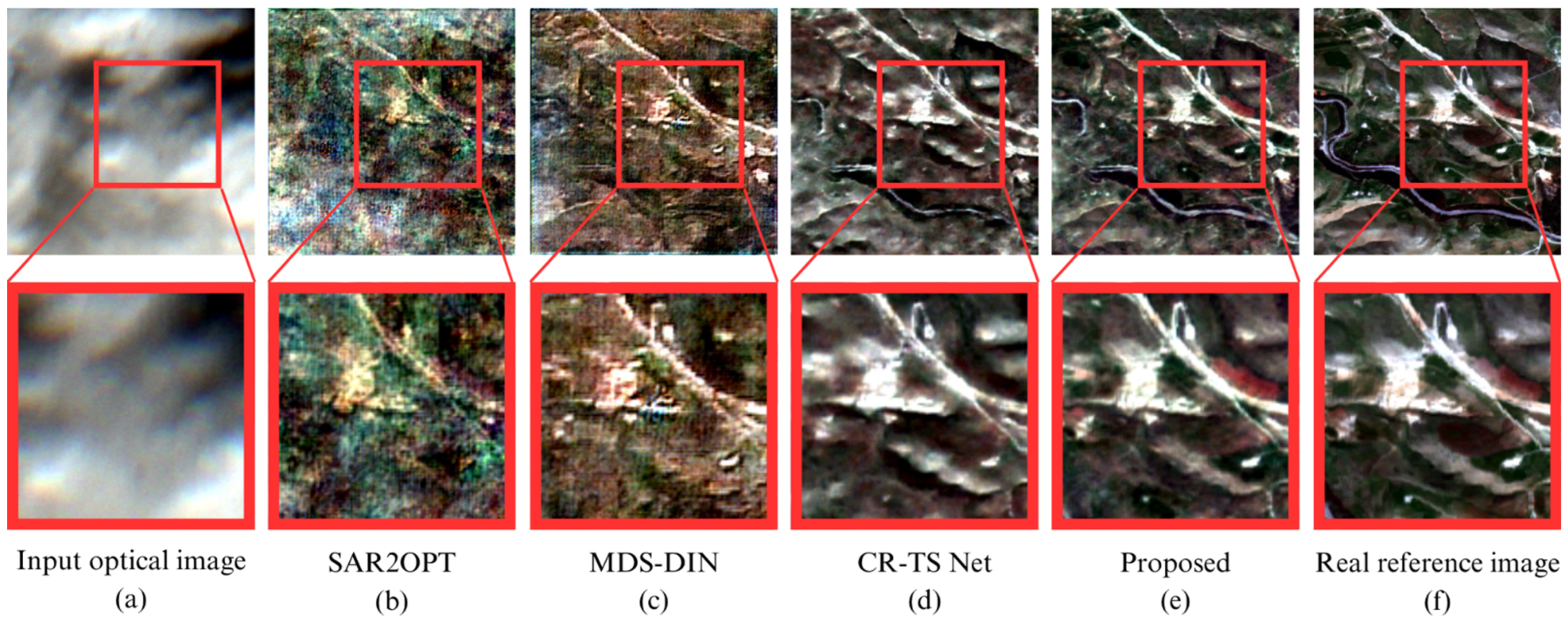
To address the challenge of insufficient utilization of spatiotemporal information in multi-temporal SAR and optical images, we proposed a spatiotemporal interactive learning network for cloud removal based on multi-temporal SAR and optical remote sensing image fusion, which innovatively introduces a Spatiotemporal Information Interaction Module. This module consists of three key components: Temporal Feature Extraction (TFE), Spatial Feature Extraction (SFE), and Spatiotemporal Feature Fusion (SFF). To analyze the effectiveness of these three components in the process of cloud removal through temporal data fusion, we alternately ablated these three parts in the original model to obtain three ablation models. Then, we compared the results of these ablation models and the original model on both real and simulated datasets to analyze the importance of each component.

The ablation study results on the simulated thin cloud and simulated thick cloud datasets are presented in

Table 1. Ablation study on the simulated thin cloud dataset. Directional arrows (↑/↓) denote optimization objectives: ↑ indicates higher values are preferred, while ↓ signifies lower values are better. The bold text indicates the best results.

Method	RMSE ↓	MAE ↓	PSNR ↑	SAM ↓	SSIM ↑
w/o SFE	0.0454	0.0155	33.2293	0.0432	0.9671
w/o TFE	0.0426	0.0196	33.5500	0.0426	0.9593
w/o SFF	0.0359	0.0225	34.1668	0.0458	0.9549
Proposed	0.0261	0.0123	34.2772	0.0421	0.9740

and

Table 2. Ablation study on the simulated thick cloud dataset. Directional arrows (↑/↓) denote optimization objectives: ↑ indicates higher values are preferred, while ↓ signifies lower values are better. The bold text indicates the best results.

Method	RMSE ↓	MAE ↓	PSNR ↑	SAM ↓	SSIM ↑
w/o SFE	0.0682	0.0336	24.4828	0.0762	0.9005
w/o TFE	0.0697	0.0426	23.8716	0.0766	0.8922
w/o SFF	0.0652	0.0335	24.4379	0.0783	0.8950
Proposed	0.0625	0.0328	24.8952	0.0755	0.9155

, respectively. It shows that on both simulated datasets, removing any of the Spatial Feature Extraction, Temporal Feature Extraction, or Spatiotemporal Feature Fusion modules leads to inferior performance across all evaluation metrics compared to the complete method. The results of independent samples t-tests show a statistically significant decline (p < 0.05) for most of the metrics. These results indicate that each component we designed plays an indispensable and critical role in effectively extracting and fusing spatiotemporal information.

As shown in

Table 3. Ablation study on the real dataset. Directional arrows (↑/↓) denote optimization objectives: ↑ indicates higher values are preferred, while ↓ signifies lower values are better. The bold text indicates the best results.

Method	AvgRMSE ↓	AvgMAE ↓	AvgPSNR ↑	AvgSAM ↓	AvgSSIM ↑
w/o SFE	0.0172	0.0115	36.3614	0.0493	0.9529
w/o TFE	0.0172	0.0116	36.4248	0.0462	0.9553
w/o SFF	0.0177	0.0115	36.1311	0.0446	0.9562
Proposed	0.0165	0.0107	37.0414	0.0446	0.9566

, the ablation experiment results on the real dataset demonstrate that removing any single component leads to a decline in model performance across multiple evaluation metrics. This performance degradation exhibits statistical significance (p < 0.05) for most metrics. These findings indicate that in real experiments, each component of our proposed spatiotemporal information interaction module actively contributes to improving overall cloud removal effectiveness.

The ablation study results from both real and simulated datasets demonstrate that the three core components within our innovatively proposed Spatiotemporal Information Interaction Module, namely Temporal Feature Extraction, Spatial Feature Extraction, and Spatiotemporal Feature Fusion, all play crucial roles in enhancing the performance of synergistic cloud removal using multi-temporal SAR and optical imagery.

6. Results

6.1. Results on Simulated Dataset

We conducted comparative experiments on simulated thick cloud and simulated thin cloud datasets. Our method employs a many-to-many cloud removal approach (generating three cloud-free images), in contrast to baseline methods which are confined to many-to-one processing (producing single output). Therefore, the generated cloud-free images of the compared methods at the same temporal phase are utilized for performance comparisons.

The overall visual results of the compared methods on the simulated thin and thick cloud datasets are shown in Figure 4 and Figure 5. It demonstrates that the results of SAR2OPT and MDS-DIN methods exhibit limitations characterized by inadequate spatial resolution and pronounced spectral distortion, leading to suboptimal overall reconstruction quality. In contrast, both the CR-TS Net and the proposed method produce reconstructed images with well-preserved spatial details, accurate color reproduction, and maintained structural integrity, exhibiting nearly equivalent overall visual quality.

For detailed comparison, we magnified the red-boxed regions in the overall visual results, enabling clear evaluation of detail reconstruction performance. Under thin cloud contamination, both CR-TS Net and the proposed method exhibit excellent cloud removal results. However, under thick cloud contamination, CR-TS Net exhibits significant deviations in restoring ground details in farmland areas, whereas the proposed method reconstructs the true state of agricultural landscapes more accurately, achieving superior clarity and accuracy in surface feature reconstruction.

The quantitative results of the comparative methods on the simulated thick and thin cloud datasets are shown in

Table 4. Comparative evaluation of four cloud removal methods using objective metrics on the simulated thin cloud dataset. Directional arrows (↑/↓) denote optimization objectives: ↑ indicates higher values are preferred, while ↓ signifies lower values are better. The bold text indicates the best results.

Method	RMSE ↓	MAE ↓	PSNR ↑	SAM ↓	SSIM ↑
SAR2OPT	0.0652	0.0367	27.4452	0.1640	0.6847
MDS-DIN	0.0671	0.0275	27.5020	0.1496	0.8358
CR-TS Net	0.0467	0.0196	32.0026	0.0425	0.9482
Proposed	0.0261	0.0123	34.2772	0.0421	0.9740

and

Table 5. Comparative evaluation of four cloud removal methods using objective metrics on the simulated thick cloud dataset. Directional arrows (↑/↓) denote optimization objectives: ↑ indicates higher values are preferred, while ↓ signifies lower values are better. The bold text indicates the best results.

Method	RMSE ↓	MAE ↓	PSNR ↑	SAM ↓	SSIM ↑
SAR2OPT	0.1095	0.0676	19.2126	0.1936	0.6185
MDS-DIN	0.1223	0.0580	18.2531	0.2389	0.6816
CR-TS Net	0.0783	0.0396	23.4417	0.0752	0.8989
Proposed	0.0625	0.0328	24.8952	0.0755	0.9155

. It demonstrates that the proposed method achieves improvements across most evaluation metrics for both simulated thin and thick cloud removal. We also applied significance testing on the results to validate the superiority of the proposed method. The results show that the proposed method displays better performance in terms of RMSE, MAE, PSNR, and SSIM (p < 0.001) on both simulated thin and thick cloud test sets, which confirms the superiority of the proposed method in terms of radiometric accuracy and noise suppression. These results also show that heavy cloud coverage significantly impacts the performance of cloud removal methods.

The experimental results on the simulated datasets above demonstrate that our method shows excellent performance in the accuracy of reconstructed details and spectral fidelity.

6.2. Results on Real Dataset

In the real experiments, we carefully selected thin cloud contaminated images and thick cloud contaminated images to construct thin cloud and thick cloud datasets, respectively. The two datasets and the complete dataset are separately utilized as test datasets to evaluate the proposed method in diverse cloud contamination scenarios.

The visual results of the compared methods under thin cloud contamination are presented in Figure 6. It shows that all methods demonstrate satisfactory overall reconstruction performance under thin cloud contamination. However, the proposed method exhibits superior restoration effects particularly in the agricultural areas marked by red bounding boxes. CR-TS Net successfully recovers bare soil information, but the internal soil patches appear indistinct. In contrast, the proposed method achieves more accurate color representation, and simultaneously preserves richer textural details and structural features. The quantitative results of the comparative methods are presented in

Table 6. Comparative evaluation of four cloud removal methods using objective metrics on the real thin cloud dataset. Directional arrows (↑/↓) denote optimization objectives: ↑ indicates higher values are preferred, while ↓ signifies lower values are better. The bold text indicates the best results.

Method	RMSE ↓	MAE ↓	PSNR ↑	SAM ↓	SSIM ↑
SAR2OPT	0.0349	0.0266	29.7669	0.0816	0.9174
MDS-DIN	0.0461	0.0365	27.8260	0.0912	0.9124
CR-TS Net	0.0183	0.0131	35.8360	0.0382	0.9673
Proposed	0.0166	0.0118	36.7376	0.0367	0.9672

. The results indicate that the proposed method achieves improvements across most evaluation metrics, with significant improvements observed in RMSE, MAE, and PSNR (p < 0.05).

The visual results under thick cloud contaminated regions are depicted in Figure 7. It shows that the presence of thick clouds poses greater challenges for cloud removal. Despite these difficulties, the proposed method consistently demonstrates superior performance. The CR-TS Net method also achieved outstanding road information reconstruction, but showed limited capability in recovering bare soil and mountainous terrain features. In contrast, the proposed method not only achieves more accurate recovery of vegetation, bare soil, and topographic features, but also restores finer texture details. The quantitative results of the comparative methods on the real thick cloud dataset, as shown in

Table 7. Comparative evaluation of four cloud removal methods using objective metrics on the real thick cloud dataset. Directional arrows (↑/↓) indicate optimization objectives: ↑ denotes that larger values are preferred, and ↓ signifies that smaller values are better. The bold text indicates the best results.

Method	RMSE ↓	MAE ↓	PSNR ↑	SAM ↓	SSIM ↑
SAR2OPT	0.0568	0.0402	25.2901	0.1649	0.7651
MDS-DIN	0.0448	0.0331	27.2584	0.1409	0.8315
CR-TS Net	0.0348	0.0239	29.7228	0.1018	0.8771
Proposed	0.0326	0.0221	30.3208	0.0976	0.8823

, indicate that our method achieves improvements across all evaluation metrics. Significant improvements are observed in RMSE, MAE, and SAM (p < 0.05).

The proposed method adopts a many-to-many cloud removal approach (generating three cloud-free outputs), unlike baseline methods limited to many-to-one processing (single output). We averaged evaluation metrics across all three outputs for performance assessment on the complete dataset. The results are shown in

Table 8. Comparative evaluation of four cloud removal methods using objective metrics on the real datasets. Directional arrows (↑/↓) indicate optimization objectives: ↑ denotes that larger values are preferred, and ↓ signifies that smaller values are better. The bold text indicates the best results.

Method	AvgRMSE ↓	AvgMAE ↓	AvgPSNR ↑	AvgSAM ↓	AvgSSIM ↑
SAR2OPT	0.0392	0.0290	28.7630	0.1041	0.8887
MDS-DIN	0.0413	0.0311	29.0451	0.0985	0.9045
CR-TS Net	0.0179	0.0112	36.2380	0.0482	0.9548
Proposed	0.0165	0.0107	37.0414	0.0446	0.9566

. It demonstrates that both the SAR2OPT method and MDS-DIN method demonstrated inferior performance across all evaluation metrics. Although the CR-TS Net achieved results comparable to the proposed method, the latter demonstrated superior performance in the RMSE, PSNR, and SAM metrics (p < 0.05).

To demonstrate the temporal reconstruction capability of the proposed method, we conducted a comprehensive visual assessment using multi-temporal image sequences from two representative regions (Figure 8). In each region, the optical images of three temporal phases systematically contain thin clouds, thick clouds, thereby thoroughly evaluating method performance across diverse cloud contamination types. The visual results are demonstrated in Figure 8. The cloud-free optical images generated by the proposed method show well-preserved structural integrity and spectral fidelity that closely approximate the reference images. Notably, the reconstructed optical images exhibit high temporal consistency with reference images at corresponding temporal phases, demonstrating its capability to capture temporal dynamics of ground features accurately and restore temporal information precisely.

The experimental results on real datasets demonstrate that our method achieved outstanding performance in terms of accuracy of reconstructed details and spectral fidelity. Moreover, the proposed method shows high temporal consistency between the reconstructed time-series optical images and reference images. It indicates that the proposed method can accurately capture the temporal dynamics of ground features and precisely restore temporal information, which is of significant importance in many-to-many cloud removal tasks.

To evaluate the efficiency and complexity of the compared methods, the training time, testing time, and parameter counts are presented in

Table 9. Comparison of training time, testing time, and parameter counts for four methods.

Method	Training Time	Testing Time	Parameters
SAR2OPT	58 h 7 min	7 m 2 s	54.462 M
MDS-DIN	58 h 29 min	8 m 18 s	54.462 M
CR-TS Net	76 h 6 min	8 m 2 s	38.474 M
Proposed	82 h 9 min	9 m 4 s	38.619 M

. SAR2OPT and MDS-DIN have similar training durations and parameter counts. CR-TS Net has a longer training time but a smaller parameter count. The proposed method has slightly higher training and testing times, with a parameter count comparable to CR-TS Net and lower than the former two. Overall, the moderate increase in computational time for the proposed method yields improvements in reconstruction accuracy, spectral fidelity, and temporal consistency, achieving a good balance between performance and efficiency.

6.3. Results on Other Regions

To investigate the generalization performance of the proposed method, we directly applied the models trained in the preceding experiments to the East Asia region. This region contains extensive urban architectural information, and its terrain, landforms, and target characteristics differ significantly from those of the African region used in previous experiments.

The visual results of the compared methods on the Asian test region are illustrated in Figure 9. In terms of overall visual effect, the cloud-removed image generated by the proposed method most closely resembles the reference image. Specifically, the morphology and extent of river areas are well recovered by the proposed method; however, it is difficult to distinguish river areas from the results of the compared methods. Furthermore, the proposed method also demonstrates superior performance in terms of spectral fidelity. Upon closer examination of the magnified details within the red box, it can be observed that our method successfully reconstructs the building outlines and basic structures in the region. In contrast, other comparative methods show unsatisfactory restoration effects for buildings, with severe loss of details. These results fully demonstrate that our method exhibits better generalization performance.

The quantitative results of the compared methods in the Asian region are presented in

Table 10. Comparative evaluation of four cloud removal methods using objective metrics on the East Asia dataset. Directional arrows (↑/↓) indicate optimization objectives: ↑ denotes that larger values are preferred, and ↓ signifies that smaller values are better. The bold text indicates the best results.

Method	RMSE ↓	MAE ↓	PSNR ↑	SAM ↓	SSIM ↑
SAR2OPT	0.2292	0.2162	12.3045	1.8789	0.3392
MDS-DIN	0.0529	0.0398	27.1005	0.2019	0.7857
CR-TS Net	0.0431	0.0333	27.0384	0.1862	0.7739
Proposed	0.0404	0.0314	28.1758	0.1766	0.7767

. Due to significant differences in terrain, landforms, and land cover features between the Asian and African datasets, all the compared methods suffer from performance deterioration. Nevertheless, as shown in Table 10, the proposed method still demonstrates significantly superior performance in RMSE, MAE, PSNR, and SAM compared to other methods (p < 0.05). The above results show that the proposed method has better generalization performance than its counterparts.

7. Discussion

Cloud contamination critically compromises the functionality of optical remote sensing data, severely diminishing their operational value. We proposed a novel spatiotemporal feature interaction-based approach for cloud removal in multi-temporal SAR–optical imagery. Leveraging a cGAN framework, the proposed method integrates three key components: a Multi-temporal Spatiotemporal Feature Joint Extraction Module, a Spatiotemporal Information Interaction Module, and a Spatiotemporal Discriminator Module. This integrated architecture successfully achieves many-to-many mapping from cloud-contaminated SAR–optical image pairs to temporally consistent cloud-free image sequences. Comparative evaluations demonstrate substantial improvements over existing methods in the following aspects:

(a)

Deep Exploitation of Spatiotemporal Information

Conventional methods often neglect the dynamic characteristics of multi-temporal data by assuming relatively static surface features. In contrast, the proposed approach thoroughly explores temporal and spatial dimensional features through the integrated Multi-temporal Spatiotemporal Feature Joint Extraction Module and Spatiotemporal Information Interaction Module, incorporating GRUs and 3D convolutional techniques. The experimental results demonstrate improved RMSE and PSNR metrics on simulated datasets, confirming superior reconstruction accuracy and robustness under complex cloud contamination scenarios compared to existing methods.

(b)

Optimization of SAR–optical Image Fusion

SAR imagery, while frequently employed as auxiliary data for optical image cloud removal due to its cloud-penetrating capability, presents fusion challenges stemming from fundamental imaging disparities with optical data. The proposed method achieves significant fusion enhancement through the Spatiotemporal Information Interaction Module, which optimizes feature integration via GRU networks while preserving spatial details through 3D convolutional operations. Visual assessments demonstrate that in mountainous regions with thick cloud cover, the proposed method outperforms CR-TS Net in terms of the reconstruction accuracy of vegetation patterns and topographic features.

(c)

Temporal Consistency

The proposed many-to-many cloud removal method demonstrates exceptional performance in maintaining temporal consistency for time-series optical image reconstruction. On real datasets, the SSIM is improved from 0.9548 (achieved by CR-TS Net) to 0.9566. Multi-temporal visual assessments reveal that the proposed method can reconstruct agricultural field boundaries and crop growth patterns with high consistency. The proposed method not only surpasses existing benchmark methods in single-temporal reconstruction but also provides reliable support for time-series analysis applications such as agricultural monitoring.

Although the proposed method has shown superior performance in cloud removal tasks, there still exist several limitations. We only selected SAR and optical images from three temporal phases for experimentation due to the available datasets. For cloud removal in time-series data, three temporal samples may be insufficient. Similar to most current SAR-based cloud removal methods, the proposed method utilizes only the amplitude information from SAR data. SAR phase information precisely records the propagation path difference in the radar wave from transmission to reception. However, it is not typically employed as an input in mainstream cloud removal tasks. In future work, we will explore the potential of using SAR phase information to assist in the cloud removal process. Moreover, we focus on features in the spatiotemporal domain, neglecting features in the frequency domain which may provide additional information for cloud removal. In future work, a joint spatiotemporal-frequency-domain feature extraction method will be considered, and datasets with more temporal phases will be utilized for performance evaluation.

8. Conclusions

To address the challenges of insufficient utilization of inherent spatiotemporal information in multi-temporal SAR and optical data, as well as the difficulties in achieving effective optical-SAR image fusion, a multi-temporal SAR–optical image fusion cloud removal framework based on spatiotemporal information was proposed in this paper. Based on cGAN architecture, we constructed a spatiotemporal interactive learning network to achieve “many-to-many” cloud removal by exploiting SAR–optical image fusion. A novel spatiotemporal information interaction module is proposed to address the inadequate utilization of spatiotemporal information in multi-temporal SAR and optical images. The proposed method was tested and verified on the open benchmark SEN12MS-CR-TS dataset. The experimental results demonstrate exceptional performance in real cloud removal tasks under both thin and thick cloud contamination scenarios. It outperforms the compared methods in terms of structural integrity, detail preservation, and color restoration.

References

1. King, M.D.; Platnick, S.; Menzel, W.P.; Ackerman, S.A.; Hubanks, P.A. Spatial and temporal distribution of clouds observed by MODIS onboard the Terra and Aqua satellites. IEEE Trans. Geosci. Remote Sens. 2013, 51, 3826–3852. [Google Scholar] [CrossRef]
2. Dian, R.; Li, S.; Sun, B.; Guo, A. Recent advances and new guidelines on hyperspectral and multispectral image fusion. Inf. Fusion 2021, 69, 40–51. [Google Scholar] [CrossRef]
3. Hong, D.; Yokoya, N.; Chanussot, J.; Zhu, X.X. An augmented linear mixing model to address spectral variability for hyperspectral unmixing. IEEE Trans. Image Process. 2018, 28, 1923–1938. [Google Scholar] [CrossRef]
4. Zhuang, L.; Ng, M.K.; Liu, Y. Cross-track illumination correction for hyperspectral pushbroom sensor images using low-rank and sparse representations. IEEE Trans. Geosci. Remote Sens. 2023, 61, 5502117. [Google Scholar] [CrossRef]
5. Maalouf, A.; Carré, P.; Augereau, B.; Fernandez-Maloigne, C. A bandelet-based inpainting technique for clouds removal from remotely sensed images. IEEE Trans. Geosci. Remote Sens. 2009, 47, 2363–2371. [Google Scholar] [CrossRef]
6. Li, X.; Shen, H.; Zhang, L.; Zhang, H.; Yuan, Q.; Yang, G. Recovering quantitative remote sensing products contaminated by thick clouds and shadows using multitemporal dictionary learning. IEEE Trans. Geosci. Remote Sens. 2014, 52, 7086–7098. [Google Scholar]
7. Li, X.; Wang, L.; Cheng, Q.; Wu, P.; Gan, W.; Fang, L. Cloud removal in remote sensing images using nonnegative matrix factorization and error correction. ISPRS J. Photogramm. Remote Sens. 2019, 148, 103–113. [Google Scholar] [CrossRef]
8. Shen, H.; Wu, J.; Cheng, Q.; Aihemaiti, M.; Zhang, C.; Li, Z. A spatiotemporal fusion based cloud removal method for remote sensing images with land cover changes. IEEE J. Sel. Top. Appl. Earth Obs. Remote Sens. 2019, 12, 862–874. [Google Scholar] [CrossRef]
9. Li, W.; Li, Y.; Chan, J.C.-W. Thick cloud removal with optical and SAR imagery via convolutional-mapping-deconvolutional network. IEEE Trans. Geosci. Remote Sens. 2019, 58, 2865–2879. [Google Scholar] [CrossRef]
10. Hoan, N.T.; Tateishi, R. Cloud removal of optical image using SAR data for ALOS applications. Experimenting on simulated ALOS data. J. Remote Sens. Soc. Jpn. 2009, 29, 410–417. [Google Scholar]
11. Chen, J.; Jönsson, P.; Tamura, M.; Gu, Z.; Matsushita, B.; Eklundh, L. A simple method for reconstructing a high-quality NDVI time-series data set based on the Savitzky–Golay filter. Remote Sens. Environ. 2004, 91, 332–344. [Google Scholar] [CrossRef]
12. Liu, L.; Lei, B. Can SAR images and optical images transfer with each other? In Proceedings of the IGARSS 2018 IEEE International Geoscience and Remote Sensing Symposium, Valencia, Spain, 22–27 July 2018; pp. 7019–7022. [Google Scholar]
13. Fuentes Reyes, M.; Auer, S.; Merkle, N.; Henry, C.; Schmitt, M. SAR-to-optical image translation based on conditional generative adversarial networks—Optimization, opportunities and limits. Remote Sens. 2019, 11, 2067. [Google Scholar] [CrossRef]
14. Mendez-Rial, R.; Calvino-Cancela, M.; Martin-Herrero, J. Anisotropic inpainting of the hypercube. IEEE Geosci. Remote Sens. Lett. 2011, 9, 214–218. [Google Scholar] [CrossRef]
15. Shen, H.; Zhang, L. A MAP-based algorithm for destriping and inpainting of remotely sensed images. IEEE Trans. Geosci. Remote Sens. 2008, 47, 1492–1502. [Google Scholar] [CrossRef]
16. Cheng, Q.; Shen, H.; Zhang, L.; Li, P. Inpainting for remotely sensed images with a multichannel nonlocal total variation model. IEEE Trans. Geosci. Remote Sens. 2013, 52, 175–187. [Google Scholar] [CrossRef]
17. Lin, C.-H.; Tsai, P.-H.; Lai, K.-H.; Chen, J.-Y. Cloud removal from multitemporal satellite images using information cloning. IEEE Trans. Geosci. Remote Sens. 2012, 51, 232–241. [Google Scholar] [CrossRef]
18. Zeng, C.; Shen, H.; Zhang, L. Recovering missing pixels for Landsat ETM+ SLC-off imagery using multi-temporal regression analysis and a regularization method. Remote Sens. Environ. 2013, 131, 182–194. [Google Scholar] [CrossRef]
19. Goodfellow, I.; Pouget-Abadie, J.; Mirza, M.; Xu, B.; Warde-Farley, D.; Ozair, S.; Courville, A.; Bengio, Y. Generative Adversarial Networks. Commun. ACM 2020, 63, 139–144. [Google Scholar] [CrossRef]
20. Li, Z.; Shen, H.; Cheng, Q.; Li, W.; Zhang, L. Thick cloud removal in high-resolution satellite images using stepwise radiometric adjustment and residual correction. Remote Sens. 2019, 11, 1925. [Google Scholar] [CrossRef]
21. Lorenzi, L.; Melgani, F.; Mercier, G. Missing-area reconstruction in multispectral images under a compressive sensing perspective. IEEE Trans. Geosci. Remote Sens. 2013, 51, 3998–4008. [Google Scholar] [CrossRef]
22. Li, J.; Wu, Z.C.; Hu, Z.W.; Zhang, J.Q.; Li, M.L.; Mo, L.; Molinier, M. Thin cloud removal in optical remote sensing images based on generative adversarial networks and physical model of cloud distortion. ISPRS J. Photogramm. Remote Sens. 2020, 166, 373–389. [Google Scholar] [CrossRef]
23. Enomoto, K.; Sakurada, K.; Wang, W.; Fukui, H.; Matsuoka, M.; Nakamura, R.; Kawaguchi, N. Filmy cloud removal on satellite imagery with multispectral conditional generative adversarial nets. In Proceedings of the IEEE Conference on Computer Vision and Pattern Recognition Workshops, Honolulu, HI, USA, 21–26 July 2017; pp. 48–56. [Google Scholar]
24. Ng, M.K.-P.; Yuan, Q.; Yan, L.; Sun, J. An adaptive weighted tensor completion method for the recovery of remote sensing images with missing data. IEEE Trans. Geosci. Remote Sens. 2017, 55, 3367–3381. [Google Scholar] [CrossRef]
25. Ji, T.-Y.; Yokoya, N.; Zhu, X.X.; Huang, T.-Z. Nonlocal tensor completion for multitemporal remotely sensed images’ inpainting. IEEE Trans. Geosci. Remote Sens. 2018, 56, 3047–3061. [Google Scholar] [CrossRef]
26. Lin, J.; Huang, T.-Z.; Zhao, X.-L.; Chen, Y.; Zhang, Q.; Yuan, Q. Robust thick cloud removal for multitemporal remote sensing images using coupled tensor factorization. IEEE Trans. Geosci. Remote Sens. 2022, 60, 5406916. [Google Scholar] [CrossRef]
27. Liu, J.; Musialski, P.; Wonka, P.; Ye, J. Tensor completion for estimating missing values in visual data. IEEE Transactions on Pattern Analysis and Machine Intelligence 2012, 35, 208–220. [Google Scholar] [CrossRef]
28. He, W.; Yokoya, N.; Yuan, L.; Zhao, Q. Remote sensing image reconstruction using tensor ring completion and total variation. IEEE Trans. Geosci. Remote Sens. 2019, 57, 8998–9009. [Google Scholar] [CrossRef]
29. Bamler, R. Principles of synthetic aperture radar. Surv. Geophys. 2000, 21, 147–157. [Google Scholar] [CrossRef]
30. Bermudez, J.D.; Happ, P.N.; Oliveira, D.A.B.; Feitosa, R.Q. SAR to optical image synthesis for cloud removal with generative adversarial networks. ISPRS Ann. Photogramm. Remote Sens. Spat. Inf. Sci. 2018, 4, 5–11. [Google Scholar] [CrossRef]
31. Darbaghshahi, F.N.; Mohammadi, M.R.; Soryani, M. Cloud removal in remote sensing images using generative adversarial networks and SAR-to-optical image translation. IEEE Trans. Geosci. Remote Sens. 2021, 60, 4105309. [Google Scholar] [CrossRef]
32. Xu, F.; Shi, Y.; Ebel, P.; Yu, L.; Xia, G.-S.; Yang, W.; Zhu, X.X. GLF-CR: SAR-enhanced cloud removal with global–local fusion. ISPRS J. Photogramm. Remote Sens. 2022, 192, 268–278. [Google Scholar] [CrossRef]
33. Huang, B.; Li, Y.; Han, X.; Cui, Y.; Li, W.; Li, R. Cloud removal from optical satellite imagery with SAR imagery using sparse representation. IEEE Geosci. Remote Sens. Lett. 2015, 12, 1046–1050. [Google Scholar] [CrossRef]
34. Grohnfeldt, C.; Schmitt, M.; Zhu, X. A conditional generative adversarial network to fuse SAR and multispectral optical data for cloud removal from Sentinel-2 images. In Proceedings of the IGARSS 2018 IEEE International Geoscience and Remote Sensing Symposium, Valencia, Spain, 22–27 July 2018; pp. 1726–1729. [Google Scholar]
35. Meraner, A.; Ebel, P.; Zhu, X.X.; Schmitt, M. Cloud removal in Sentinel-2 imagery using a deep residual neural network and SAR-optical data fusion. ISPRS J. Photogramm. Remote Sens. 2020, 166, 333–346. [Google Scholar] [CrossRef] [PubMed]
36. He, W.; Yokoya, N. Multi-temporal sentinel-1 and-2 data fusion for optical image simulation. ISPRS Int. J. Geo-Inf. 2018, 7, 389. [Google Scholar] [CrossRef]
37. Bermudez, J.D.; Happ, P.N.; Feitosa, R.Q.; Oliveira, D.A. Synthesis of multispectral optical images from SAR/optical multitemporal data using conditional generative adversarial networks. IEEE Geosci. Remote Sens. Lett. 2019, 16, 1220–1224. [Google Scholar] [CrossRef]
38. Xia, Y.; Zhang, H.; Zhang, L.; Fan, Z. Cloud removal of optical remote sensing imagery with multitemporal SAR-optical data using X-Mtgan. In Proceedings of the IGARSS 2019 IEEE International Geoscience and Remote Sensing Symposium, Yokohama, Japan, 28 July–2 August 2019; pp. 3396–3399. [Google Scholar]
39. Gao, J.; Yuan, Q.; Li, J.; Zhang, H.; Su, X. Cloud removal with fusion of high resolution optical and SAR images using generative adversarial networks. Remote Sens. 2020, 12, 191. [Google Scholar] [CrossRef]
40. Isola, P.; Zhu, J.-Y.; Zhou, T.; Efros, A.A. Image-to-image translation with conditional adversarial networks. In Proceedings of the IEEE Conference on Computer Vision and Pattern Recognition, Honolulu, HI, USA, 21–26 July 2017; pp. 1125–1134. [Google Scholar]
41. Sarukkai, V.; Jain, A.; Uzkent, B.; Ermon, S. Cloud removal from satellite images using spatiotemporal generator networks. In Proceedings of the IEEE/CVF Winter Conference on Applications of Computer Vision, Snowmass Village, CO, USA, 1–5 March 2020; pp. 1796–1805. [Google Scholar]
42. Huang, G.-L.; Wu, P.-Y. CTGAN: Cloud transformer generative adversarial network. In Proceedings of the 2022 IEEE International Conference on Image Processing (ICIP), Bordeaux, France, 16–19 October 2022; pp. 511–515. [Google Scholar]
43. Ma, X.; Huang, Y.; Zhang, X.; Pun, M.-O.; Huang, B. Cloud-egan: Rethinking cyclegan from a feature enhancement perspective for cloud removal by combining cnn and transformer. IEEE J. Sel. Top. Appl. Earth Obs. Remote Sens. 2023, 16, 4999–5012. [Google Scholar] [CrossRef]
44. Chen, B.; Huang, B.; Chen, L.; Xu, B. Spatially and temporally weighted regression: A novel method to produce continuous cloud-free Landsat imagery. IEEE Trans. Geosci. Remote Sens. 2016, 55, 27–37. [Google Scholar] [CrossRef]
45. Wen, X.; Pan, Z.; Hu, Y.; Liu, J. An effective network integrating residual learning and channel attention mechanism for thin cloud removal. IEEE Geosci. Remote Sens. Lett. 2022, 19, 6507605. [Google Scholar] [CrossRef]
46. Ji, S.; Xu, W.; Yang, M.; Yu, K. 3D convolutional neural networks for human action recognition. IEEE Trans. Pattern Anal. Mach. Intell. 2012, 35, 221–231. [Google Scholar] [CrossRef]
47. Szegedy, C.; Ioffe, S.; Vanhoucke, V.; Alemi, A. Inception-v4, inception-resnet and the impact of residual connections on learning. In Proceedings of the AAAI Conference on Artificial Intelligence, San Francisco, CA, USA, 4–9 February 2017. [Google Scholar]
48. Chung, J.; Gulcehre, C.; Cho, K.; Bengio, Y. Empirical evaluation of gated recurrent neural networks on sequence modeling. In Proceedings of the NIPS 2014 Workshop on Deep Learning, Montreal, QC, Canada, 13 December 2014. [Google Scholar]
49. Miyato, T.; Kataoka, T.; Koyama, M.; Yoshida, Y. Spectral Normalization for Generative Adversarial Networks. In Proceedings of the International Conference on Learning Representations, Vancouver, BC, Canada, 30 April–3 May 2018. [Google Scholar]
50. Wang, Z.; Bovik, A.C.; Sheikh, H.R.; Simoncelli, E.P. Image quality assessment: From error visibility to structural similarity. IEEE Trans. Image Process. 2004, 13, 600–612. [Google Scholar] [CrossRef]
51. Ebel, P.; Xu, Y.; Schmitt, M.; Zhu, X.X. SEN12MS-CR-TS: A remote-sensing data set for multimodal multitemporal cloud removal. IEEE Trans. Geosci. Remote Sens. 2022, 60, 1–14. [Google Scholar] [CrossRef]
52. Veci, L.; Prats-Iraola, P.; Scheiber, R.; Collard, F.; Fomferra, N.; Engdahl, M. The Sentinel-1 Toolbox. In Proceedings of the IEEE International Geoscience and Remote Sensing Symposium (IGARSS), Quebec City, QC, Canada, 13–18 July 2014; pp. 1–3. [Google Scholar]
53. Kingma, D.P.; Ba, J. Adam: A Method for Stochastic Optimization. In Proceedings of the 3rd International Conference on Learning Representations (ICLR), San Diego, CA, USA, 7–9 May 2015. [Google Scholar]
54. Wang, Z.; Liu, Q.; Meng, X.; Jin, W. Multidiscriminator Supervision-Based Dual-Stream Interactive Network for High-Fidelity Cloud Removal on Multitemporal SAR and Optical Images. IEEE Geosci. Remote Sens. Lett. 2023, 20, 6012205. [Google Scholar] [CrossRef]
Figure 1. The structure of the overall framework of the proposed cloud removal method. S t denotes the SAR image at temporal phase t , C O t represents the cloud-contaminated optical image at the corresponding temporal phase. Output represents the generated cloud-free images.
Remotesensing 17 02169 g001
Figure 2. Structure diagram of spatiotemporal information fusion network.
Remotesensing 17 02169 g002
Figure 3. Training and validation loss curves of the model on simulated and real datasets. (a) Training and validation loss curves on the simulated dataset. (b) Training and validation loss curves on the real dataset.
Remotesensing 17 02169 g003
Figure 4. Comparative experimental results of thin cloud removal on simulated dataset. The first row displays the visualization results of the full images, while the second row presents the zoomed-in images of the red-boxed regions marked in the first row. (a) Input optical image. (b) SAR2OPT method. (c) MDS-DIN method. (d) CR-TS Net method. (e) Proposed method. (f) Real reference image.
Remotesensing 17 02169 g004
Figure 5. Comparative experimental results of thick cloud removal on simulated dataset. The first row displays the visualization results of the full images, while the second row presents the zoomed-in images of the red-boxed regions marked in the first row. (a) Input optical image. (b) SAR2OPT method. (c) MDS-DIN method. (d) CR-TS Net method. (e) Proposed method. (f) Real reference image.
Remotesensing 17 02169 g005
Figure 6. Comparative experimental results of thin cloud removal on real datasets. The first row displays the visualization results of the full images, while the second row presents the zoomed-in images of the red-boxed regions marked in the first row. (a) Input optical image (acquired on 10 March 2018). (b) SAR2OPT method. (c) MDS-DIN method. (d) CR-TS Net method. (e) Proposed method. (f) Real reference image (acquired on 20 March 2018).
Remotesensing 17 02169 g006
Figure 7. Comparative experimental results of thick cloud removal on real datasets. The first row displays the visualization results of the full images, while the second row presents the zoomed-in images of the red-boxed regions marked in the first row. (a) Input optical image (acquired on 6 January 2018). (b) SAR2OPT method. (c) MDS-DIN method. (d) CR-TS Net method. (e) Proposed method. (f) Real reference image (acquired on 21 January 2018).
Remotesensing 17 02169 g007
Figure 8. Experimental results of the proposed method at two different locations. (a1/a2) input SAR images; (b1/b2) optical images with clouds; (c1/c2) cloud-free optical images generated by the proposed method; (d1/d2) reference images. Input images were acquired on 10 March 2018 (T1), 14 April 2018 (T2), and 19 May 2018 (T3). Reference images were collected on 20 March 2018 (T1, 10-day interval), 24 April 2018 (T2, 10-day interval), and 9 May 2018 (T3, 10-day interval).
Remotesensing 17 02169 g008
Figure 9. Comparative experimental results on the East Asia dataset. The first row displays the visualization results of the full images, while the second row presents the zoomed-in images of the red-boxed regions marked in the first row. (a) Input optical image (acquired on 10 October 2018); (b) SAR2OPT method. (c) MDS-DIN method. (d) CR-TS Net method. (e) Proposed method. (f) Real reference image (acquired on 20 October 2018).
Remotesensing 17 02169 g009