Mamba-STFM: A Mamba-Based Spatiotemporal Fusion Method for Remote Sensing Images

Abstract

Spatiotemporal fusion techniques can generate remote sensing imagery with high spatial and temporal resolutions, thereby facilitating Earth observation. However, traditional methods are constrained by linear assumptions; generative adversarial networks suffer from mode collapse; convolutional neural networks struggle to capture global context; and Transformers are hard to scale due to quadratic computational complexity and high memory consumption. To address these challenges, this study introduces an end-to-end remote sensing image spatiotemporal fusion approach based on the Mamba architecture (Mamba-spatiotemporal fusion model, Mamba-STFM), marking the first application of Mamba in this domain and presenting a novel paradigm for spatiotemporal fusion model design. Mamba-STFM consists of a feature extraction encoder and a feature fusion decoder. At the core of the encoder is the visual state space-FuseCore-AttNet block (VSS-FCAN block), which deeply integrates linear complexity cross-scan global perception with a channel attention mechanism, significantly reducing quadratic-level computation and memory overhead while improving inference throughput through parallel scanning and kernel fusion techniques. The decoder’s core is the spatiotemporal mixture-of-experts fusion module (STF-MoE block), composed of our novel spatial expert and temporal expert modules. The spatial expert adaptively adjusts channel weights to optimize spatial feature representation, enabling precise alignment and fusion of multi-resolution images, while the temporal expert incorporates a temporal squeeze-and-excitation mechanism and selective state space model (SSM) techniques to efficiently capture short-range temporal dependencies, maintain linear sequence modeling complexity, and further enhance overall spatiotemporal fusion throughput. Extensive experiments on public datasets demonstrate that Mamba-STFM outperforms existing methods in fusion quality; ablation studies validate the effectiveness of each core module; and efficiency analyses and application comparisons further confirm the model’s superior performance.

1. Introduction

As a core technology for monitoring the Earth’s surface systems, remote sensing plays a fundamental role in a wide range of applications due to its broad coverage, rapid acquisition, and frequent observation capabilities. From precision agriculture [1] and dynamic environmental assessment [2,3,4] to rapid disaster response [5] and scientific urban planning [6], remote sensing data serve as a critical driving force. In these fields, the simultaneous acquisition of high-spatial resolution (HSR) and high-temporal resolution (HTR) remote sensing image time series is of paramount importance. However, existing single-platform remote sensing satellites generally face multiple limitations [7,8,9]. Constrained by cloud cover, orbital cycles, and inherent trade-offs in sensor technology, these platforms struggle to provide data with both high spatial and high temporal resolution simultaneously—an often unattainable compromise. For instance, the Landsat satellites offer spatial resolutions of approximately 25 m [10], which are sufficient for capturing surface details, yet their intrinsic 16-day revisit cycle limits their ability to meet high temporal resolution demands. In contrast, the MODIS sensor [11,12] provides near-daily or even more frequent global observations, but at the cost of spatial precision, with resolutions ranging from 250 to 1000 m.

In response to the challenge of acquiring high-spatial and high-temporal resolution data simultaneously, spatiotemporal fusion (STF) of remote sensing images has emerged [13] and evolved into a key research direction in the field of remote sensing data processing. The value of STF lies in its ability to overcome the limitations of single-sensor systems by integrating complementary data from multiple sensors [14,15]. Specifically, the technique typically uses reference pairs composed of low-spatial resolution/high-temporal resolution (LSR/HTR) images and high-spatial resolution/low-temporal resolution (HSR/LTR) images from known dates, along with a coarse image from the target prediction date, to generate a high-quality image sequence at the target date with both HSR and HTR.

After decades of exploration and development [13], spatiotemporal fusion (STF) algorithms have evolved into a diverse array of technical systems, each rooted in different forms of prior knowledge and model design philosophies. From the perspective of core principles and implementation strategies, existing algorithms can be broadly categorized into five main types: (1) weight-based methods [15,16]; (2) methods based on mixed-pixel decomposition [17,18]; (3) hybrid approaches [19]; (4) shallow learning-based methods; and (5) deep learning-based methods [20]. Among these, weight function-based methods represent some of the earliest and most widely applied techniques in the STF domain. Their key mechanism involves estimating the pixel values of the fine image on the target date by performing a weighted average of reference image pixels surrounding the target pixel. The weights are typically computed based on spatial proximity, spectral similarity, and temporal consistency. For example, the STARFM model [15], a representative algorithm in this category, assigns higher weights to spectrally and structurally similar pure pixels within a defined neighborhood. Although subsequent studies have proposed improvements in weighting strategies [21], cross-sensor adaptation [22], and method integration [23], weight-based methods still face significant challenges in improving fusion accuracy when applied to scenes with abrupt land cover changes or high spatial complexity due to their reliance on assumptions of local windows and linear relationships.

Mixed-pixel decomposition-based methods [24,25] are grounded in the understanding that low-resolution pixels are, in fact, mixtures of spectral signals from multiple high-resolution land surface components. These techniques employ spectral unmixing processes [17,18] to extract the fractional abundances of various land cover types from coarse-resolution images and then synthesize high-resolution images for the target date by incorporating spatial distributions or endmember spectral information derived from reference high-resolution imagery. While these methods offer advantages in handling sub-pixel-level land cover heterogeneity, their final accuracy is highly dependent on the adaptability of the spectral mixing model, the quality of the endmember library, and the ability to effectively capture and model temporal variations in land surface spectral properties.

To address the limitations of single-principle approaches, researchers have developed hybrid fusion strategies. These methods [19] aim to organically integrate the strengths of different techniques, including weight functions, mixed-pixel decomposition, and even change detection. In practice, FSDAF proposed by Zhu et al. [26] is a representative method that cleverly combines weight functions with mixed-pixel decomposition. Another example is CSAFM, employed by Wang et al. for evapotranspiration estimation [27], which also merges these two strategies. Furthermore, FSDAF 2.0, an improved version developed by Guo et al. [28], incorporates change detection and optimization techniques. These hybrid methods are typically more flexible in design and capable of delivering improved fusion performance. However, this often comes at the cost of increased model complexity, requiring more parameter tuning and reliance on additional assumptions.

To overcome the limitations of traditional spatiotemporal fusion algorithms—such as weight-based and mixed-pixel decomposition methods—which rely on fixed assumptions, shallow learning techniques from the domain of machine learning have been introduced as data-driven alternatives or enhancements. These approaches encompass several technical paths: Bayesian-based methods [29,30], which formulate fusion as a maximum a posteriori (MAP) inference problem by modeling temporal evolution and scale transformation; sparse representation–based methods [31], which exploit the sparsity of image patches by learning dictionaries and sparse coding relationships; and dictionary learning-based methods [32], which focus on learning paired dictionaries capable of capturing structural characteristics of images. Compared with traditional physics- or empirical model–based approaches, these shallow learning models demonstrate greater adaptability and offer moderate performance improvements. However, their relatively low model complexity and limited capacity for deep feature extraction often hinder their ability to manage complex spatiotemporal dynamics and highly heterogeneous regions. Nevertheless, their exploration of data-driven paradigms has laid a critical foundation for the subsequent application of more powerful deep learning methods in the STF domain.

Benefiting from their powerful nonlinear modeling capabilities and end-to-end learning frameworks, deep learning methods have achieved significant breakthroughs in the field of spatiotemporal fusion (STF) of remote sensing imagery, substantially raising performance ceilings and surpassing previous techniques. Deep learning models such as convolutional neural networks (CNNs), generative adversarial networks (GANs), and Transformers can autonomously learn complex nonlinear correspondences between images across different spatial and temporal scales. In CNN-based approaches, researchers have leveraged the spatial feature extraction strength of CNNs to design fusion models. Representative works include the early STFCNN [33], as well as more sophisticated architectures such as DCSTFN [34], EDCSTFN [20], the dual-stream CNN model STFNet [35], attention-augmented models [36], and BiaSTF [37], which addresses sensor biases. In parallel, GAN-based approaches [38,39,40,41] have also demonstrated outstanding performance on STF tasks. Notably, GAN-STFM [42] innovated the input paradigm by requiring only a coarse image from the target date and a fine-resolution image from any reference date to efficiently generate high-accuracy fused outputs. The Transformer architecture [43] has attracted increasing attention due to its unique self-attention mechanism, which enables direct modeling of dependencies among input elements, thereby facilitating effective global information representation. This capability is particularly critical for addressing large-scale spatial heterogeneity and complex temporal variations. Pioneering work by Liu et al. [44] introduced MSNet, which combines CNN and Transformer architectures for STF, effectively mitigating the local receptive field limitations of CNNs. This work laid the foundation for subsequent hybrid or Transformer-based fusion models such as SwinSTFM [45], CTSTFM [46], and EMSNet [47], offering crucial insights and architectural inspiration.

Despite the substantial progress achieved by deep learning–based spatiotemporal fusion (STF) methods, their practical application still faces several challenges. For CNN-based methods, a key limitation lies in their inherently local receptive field, which restricts the effective modeling of global and long-range spatial dependencies—often leading to performance bottlenecks in scenarios with large-scale surface heterogeneity or abrupt changes. Additionally, the shared weight design of convolutional layers may lack the flexibility to capture fine-grained, highly variant local patterns. GAN-based methods, on the other hand, suffer from issues related to computational efficiency and training stability. Performing generative operations directly in high-resolution space [42] is beneficial for preserving detail but comes with significant computational cost; dimensionality reduction strategies may alleviate this, but often at the expense of critical spatial information, requiring post-processing compensation. Furthermore, GAN training is notoriously unstable and prone to mode collapse [48,49], which poses significant challenges when fitting and generalizing to the complex and variable characteristics of remote sensing data. Transformer-based architectures also face distinct hurdles in STF tasks: the quadratic computational complexity of their self-attention mechanism leads to prohibitive computational and memory demands when processing high-resolution imagery; the absence of local inductive bias, as found in CNNs, hampers the accurate capture of fine textures and edges; and the need for large-scale labeled datasets conflicts with the scarcity of annotated samples in the remote sensing domain, limiting their training effectiveness. Moreover, in long-sequence modeling, self-attention mechanisms can introduce abrupt shifts and noise, necessitating the integration of temporal consistency modules to ensure stability.

To address the aforementioned limitations of existing architectures, this study introduces the Mamba architecture [50] into the domain of remote sensing spatiotemporal fusion and proposes an end-to-end method termed the Mamba-spatiotemporal fusion model (Mamba-STFM). The Mamba-STFM framework comprises a multi-branch feature extraction encoder and a multi-scale feature fusion decoder. Its core components include the visual state space–FuseCore–AttNet block (VSS–FCAN block), a spatial expert, and a temporal expert. The VSS-FCAN block is an enhanced version of the conventional visual state space (VSS) block, in which the standard Feed-Forward Network (FFN) is replaced with a FuseCore-AttNet block incorporating channel attention. The spatial expert and temporal expert are novel modules originally designed in this work. The key contributions of these core modules are as follows.

(1)

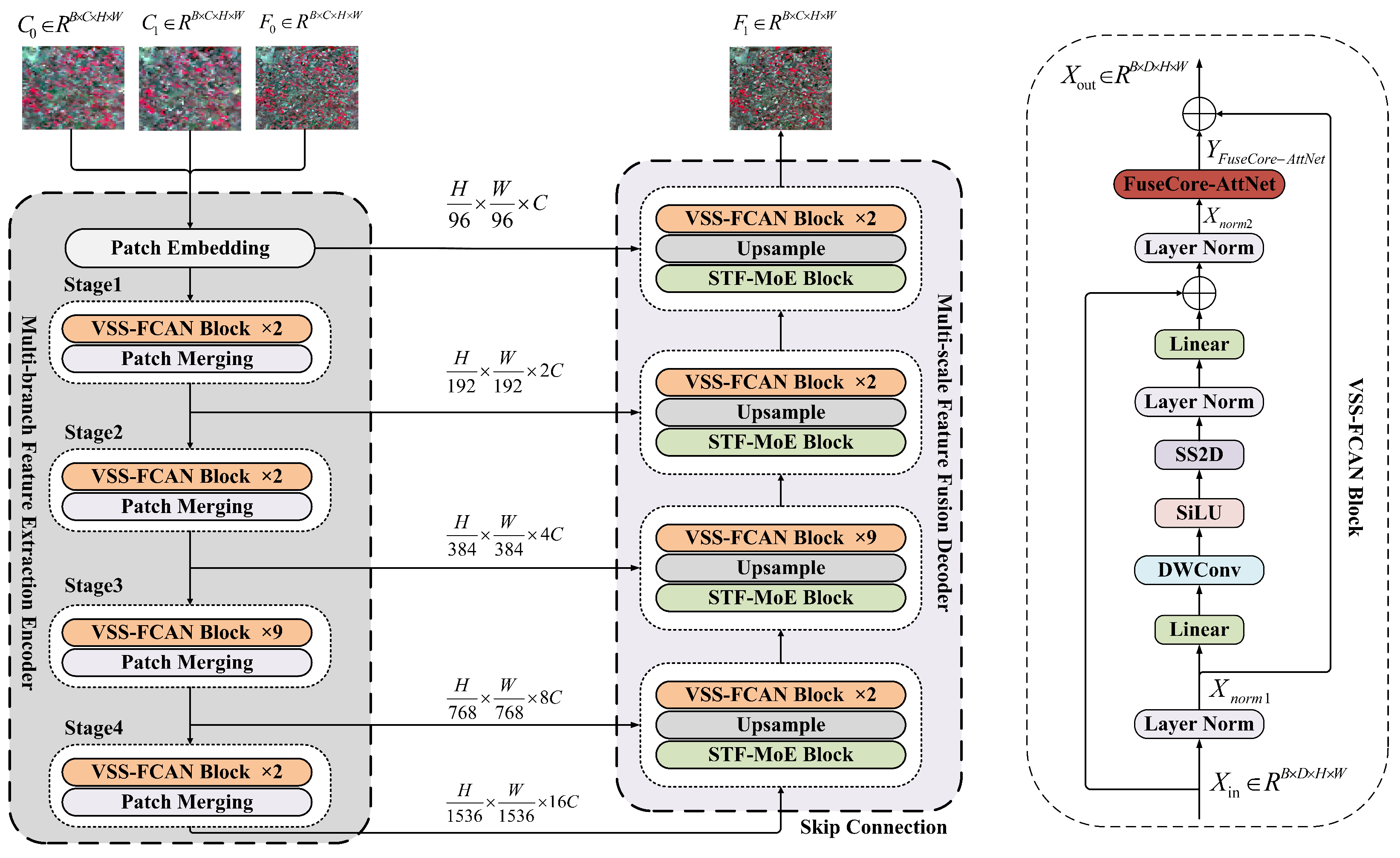
The VSS-FCAN block combines cross-scan global perception with channel attention mechanisms, significantly reducing computational and memory overhead at quadratic complexity. Additionally, it enhances model inference throughput through parallel scanning and kernel fusion techniques.

(2)

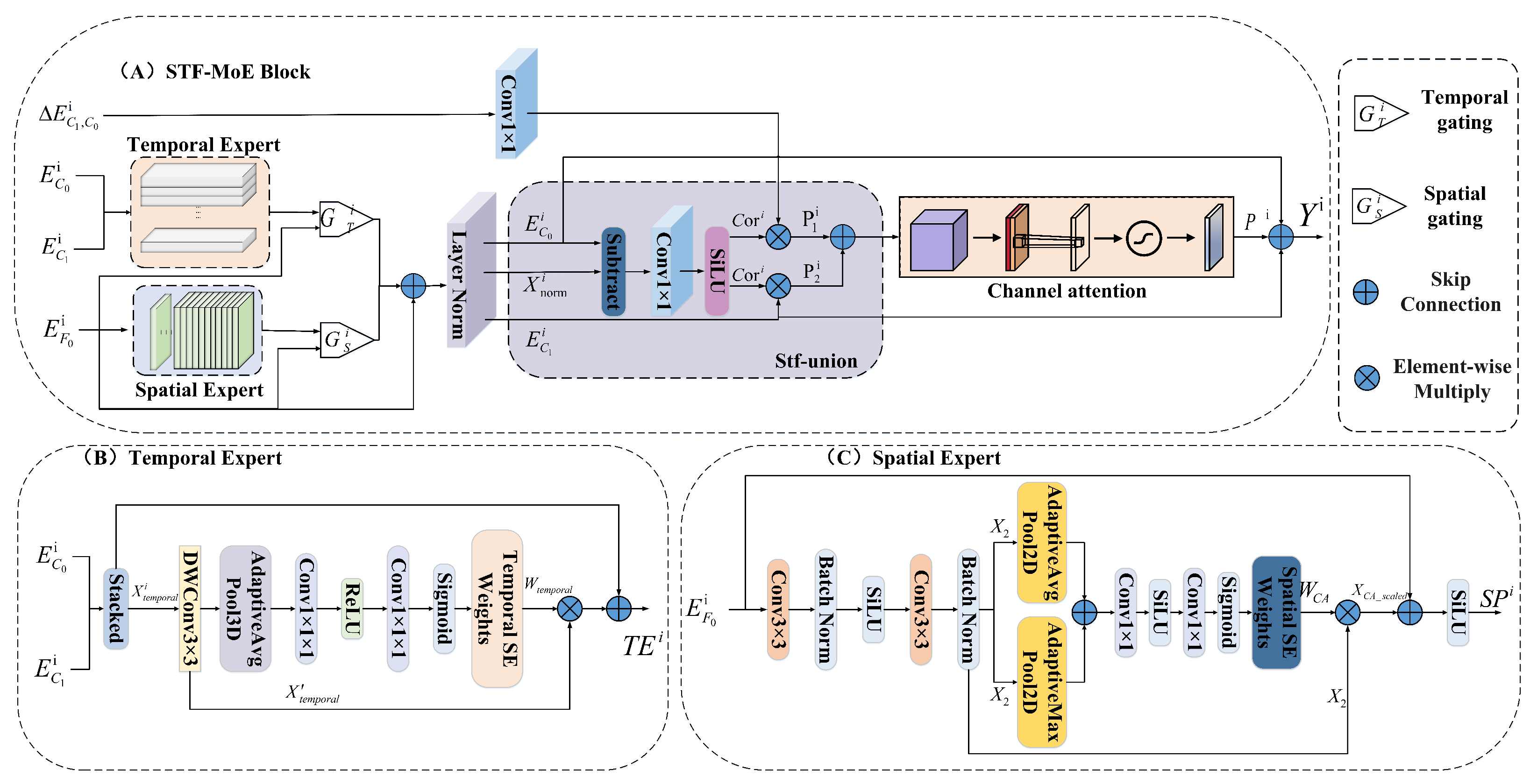
The spatial expert utilizes an enhanced 2D residual convolutional module and incorporates a channel attention mechanism, adaptively adjusting channel weights to optimize spatial feature representation, thereby achieving precise alignment and fusion of coarse and fine-resolution images.

(3)

The temporal expert introduces a 3D residual convolutional module for adjacent time steps, combining a temporal squeeze-and-excitation mechanism with selective state space model (SSM) techniques. This design efficiently captures short-range temporal dependencies while maintaining linear complexity in temporal sequence modeling, further improving the overall throughput of spatiotemporal fusion.

To comprehensively evaluate the performance of our proposed method, we compare it with several representative spatiotemporal fusion models, including both traditional and deep learning-based approaches. Among traditional methods, STARFM is the first model based on a weighting function, which predicts pixel values using spectral differences and spatial similarities, and ESTARFM improves upon it by introducing transformation coefficients that enhance the prediction of small and linear features, particularly in heterogeneous and seasonally dynamic landscapes. For deep learning-based baselines, GANSTFM is a typical GAN-based model that breaks the time constraint of reference image selection and uses switchable normalization to better capture temporal characteristics. EDCSTFN represents CNN-based models with a dual-branch structure and feature-level fusion, showing robustness to low-quality data and limited cloud coverage. Swin-STFM is the first model to apply the Swin Transformer to spatiotemporal fusion, combining spectral unmixing theory with attention-based feature extraction to enhance contextual understanding and generation quality. ECPW-STFM is the first to introduce wavelet transform into spatiotemporal image fusion, enabling separate learning of high- and low-frequency components and achieving a better balance between global structure and local detail. STFDiff is the first to employ a diffusion model for spatiotemporal fusion, progressively refining Gaussian noise into the target image through a dual-stream UNet and enhanced noise feature extraction. These baselines span classical traditional models, CNNs, GANs, Transformers, wavelet-enhanced methods, and diffusion models, providing a comprehensive benchmark to validate the effectiveness of our approach.

This Mamba-based method, equipped with a spatiotemporal expert mixture fusion module, not only offers linear computational complexity and high inference throughput but also achieves a significant performance breakthrough in spatiotemporal fusion tasks. Comparative experiments conducted on two widely used public remote sensing spatiotemporal fusion datasets demonstrate that the Mamba-STFM model outperforms existing state-of-the-art (SOTA) methods, achieving superior fusion performance.

The remainder of this paper is organized as follows: Section 2 introduces the overall architecture and core modules of Mamba-STFM; Section 3 describes the experimental design and process; Section 4 presents a series of comparisons with multiple methods on public datasets, ablation studies of Mamba-STFM, efficiency evaluations, and performance comparisons in practical applications; Section 5 discusses the results; Section 6 concludes the paper and discusses future directions.

2. Methodology

2.1. Overall Structure

The Mamba-STFM model proposed in this study is an end-to-end remote sensing spatiotemporal fusion model based on Mamba, designed to effectively integrate multi-source heterogeneous remote sensing data to generate synthesized images with high spatiotemporal resolution. The overall model adopts an encoder–decoder architecture, as shown in Figure 1, and primarily consists of a multi-branch feature extraction encoder and a multi-scale feature fusion decoder. The multi-branch feature extraction encoder is an improvement based on the Vision Mamba backbone network, while the multi-scale feature fusion decoder is composed of multiple STF-MoE blocks and VSS-FCAN blocks. The input to Mamba-STFM consists of a pair of coarse and fine images at the T0 time step and a coarse image at the T1 time step, while the output is a fine-resolution image at the T1 time step.

The multi-branch feature extraction encoder is used to process the input images and obtain multi-scale feature representations. Specifically, the input coarse image $C_0\in R^{B\times C\times H\times W}$ at the T0 time step, fine image $F_0\in R^{B\times C\times H\times W}$ at the T0 time step, and coarse image $C_1\in R^{B\times C\times H\times W}$ at the T1 time step are fed in parallel into three independent feature extraction branches, with each branch being constructed based on a hierarchical Vision Mamba structure. The input images are first processed through a patch embedding layer, which transforms them into feature tokens and expands their dimensionality. These feature tokens then pass through a series of VSS-FCAN blocks, which are adept at capturing both local and global dependencies, to perform transformation and information aggregation. During this process, spatial downsampling is applied to reduce the spatial resolution of feature maps while increasing the number of channels, thereby enabling multi-scale feature extraction. As a result, multi-scale feature lists $\left[E_{source}^i\right]$ are generated for $C_0$, $F_0$, and $C_1$, respectively, where “source” denotes the image type and “i” indicates the i-th scale. Additionally, the differences between the coarse-resolution features at T1 and T0 are computed.

$$\Delta E_{C_1,C_0}^i=E_{C_0}^i-E_{C_1}^i,i\in \left\{1,2,3,4\right\}.$$

(1)

Finally, the encoder outputs multi-scale feature lists $\left[E_{C_0}^i\right]$, $\left[\Delta E_{C_1,C_0}^i\right]$, $\left[E_{F_0}^i\right]$, and $\left[E_{C_1}^i\right]$.

The multi-scale feature fusion decoder processes the multi-scale feature lists generated by the encoder. This component is responsible for integrating multi-source and multitemporal feature information and progressively reconstructing high-resolution imagery. The process can be conceptually divided into two stages: intra-scale feature fusion and hierarchical feature reconstruction. During the intra-scale feature fusion stage, for any given scale i, the input features $\left[E_{C_0}^i\right]$, $\left[\Delta E_{C_1,C_0}^i\right]$, $\left[E_{F_0}^i\right]$, and $\left[E_{C_1}^i\right]$ are fed into a dedicated spatiotemporal mixture-of-experts fusion module (STF-MoE block). This module consists of a temporal expert pathway and a spatial expert pathway. The temporal expert handles the coarse-resolution features from T0 and T1, while the spatial expert focuses on the fine-resolution features from T0. The outputs of these experts are weighted using a dynamic gating mechanism generated based on feature $E_{F_0}^i$. The model then computes the correspondence between the enhanced features and the original features and predicts the changes in fine resolution. Multiple prediction results are aggregated and refined through channel attention. Finally, residual connections are used to integrate the original information, generating the fused feature $Y^i$ at the corresponding scale. This process is applied in parallel across all scales, resulting in a multi-scale fused feature list $\left[Y^1,Y^2,Y^3,Y^4\right]$, where C represents the fused output at scale i.

$$Y^i={ScaleFusionUnit}^i\left(E_{C_0}^i,\Delta E_{C_1,C_0}^i,E_{F_0}^i,E_{C_1}^i\right),i\in \{1,2,3,4\}.$$

(2)

These fused features are then passed into the hierarchical feature reconstruction stage, which is responsible for restoring the feature resolution to match that of the original fine-resolution image. A bottom-up strategy is employed to integrate low-resolution contextual information with fine-grained details from the current scale.

$$X_{\mathrm{combined}}^i=Y^i+\mathrm{BilinearUpsample}\left(X_{up}^{i+1}\right),i\in \{1,2,3\}.$$

(3)

Here, $X_{up}^{i+1}$ refers to the upsampled feature from scale i + 1. The combined feature $X_{combined}^i$ is further enhanced and its spatial resolution expanded through a series of upsampling and feature refinement operations. This iterative process is performed progressively across scales until a feature map matching the spatial dimensions of the original fine-resolution image is obtained. The final feature map is normalized to generate the predicted fine-resolution image at time T1, denoted as $F^1$. $X_{up}^1$ represents the highest-resolution feature prior to the final layer normalization step.

$$\begin{array}{c}\hfill F_1=\mathrm{OutputLayer}\left(\mathrm{FinalUpsample}\left(LayerNorm\left(X_{up}^1\right)\right)\right)\end{array}$$

(4)

2.2. Visual State Space-FuseCore-AttNet Block

Because the Vision Transformer (ViT) successfully introduced the Transformer architecture into the field of computer vision, self-attention-based models have achieved remarkable progress in tasks such as image classification, object detection, and semantic segmentation, demonstrating strong global feature modeling capabilities. However, the standard ViT requires images to be partitioned into fixed-size patches and flattened into sequences, leading to quadratic computational complexity with respect to image size and limited ability to capture fine-grained local structures. To address these limitations, the Swin Transformer was proposed, which incorporates a shifted window mechanism that confines self-attention computations to local windows while enabling cross-window interactions through a window-shifting strategy. The Swin Transformer effectively reduces computational complexity, making it suitable for high-resolution image processing, and its hierarchical design allows for the extraction of multi-scale features, compensating for the lack of local inductive bias in ViT. Nonetheless, the Swin Transformer still relies on explicit attention matrix computation, which remains a bottleneck when handling very long sequences or scenarios that demand higher computational efficiency.

In recent years, state space models (SSMs) have demonstrated outstanding performance and computational efficiency in sequence modeling. In particular, the introduction of the Mamba architecture has enabled efficient linear-time sequence processing through a hardware-aware selective scan mechanism. Inspired by this advancement, Vision Mamba (VMamba) extends the advantages of SSMs to visual tasks, constructing a highly efficient visual backbone network. By leveraging the selective scan mechanism of SSMs, VMamba performs efficient information aggregation over flattened image sequences, effectively capturing long-range dependencies while avoiding the quadratic computational overhead typically associated with explicit attention. This architecture exhibits superior speed and performance potential compared with existing Transformer and Transformer-like models.

Leveraging the strengths of VMamba, this study designs a multi-branch feature extraction encoder that efficiently captures multi-scale features with both global and local contextual information from the input images. The encoder consists of three independent VMamba backbone branches, each responsible for processing inputs $C_0$, $F_0$, and $C_1$, respectively. Each branch adopts a hierarchical design consisting of a patch embedding layer followed by a series of downsampling stages. The patch embedding layer transforms the input image into an initial feature sequence via convolution, simultaneously enhancing feature dimensionality and adjusting spatial structure. Each subsequent downsampling stage comprises multiple VSS-FCAN blocks and concludes with a downsampling layer (patch merging) to reduce spatial resolution while increasing channel dimensions. The VSS-FCAN block serves as the core computational unit of the encoder, as illustrated in Figure 1. It is an enhanced version of the standard VSS block, where the multilayer perceptron (MLP) feed-forward network is replaced with a convolutional feed-forward network integrated with channel attention (FuseCore-AttNet), better suited for 2D image processing. Internally, the VSS-FCAN block consists of a normalization layer, a feature transformation module based on selective scan (SS2D), and the FuseCore-AttNet. Specifically, the input feature $X_{in}\in R^{B\times C\times H\times W}$ is first normalized through a preprocessing layer.

$$\begin{array}{c}\hfill X_{norm1}=Normalize1\left(X_{in}\right)\end{array}$$

(5)

Subsequently, the normalized feature $X_{norm1}$ is passed into the SS2D module. This module applies content-aware selective state space modeling (SSM) scanning mechanisms across multiple directions—such as horizontal, vertical, and their reverse counterparts—effectively capturing spatial dependencies within the two-dimensional domain and producing output feature $Y_{SSM}\in R^{B\times C\times H\times W}$.

$$\begin{array}{c}\hfill Y_{SSM}=SS2D\left(X_{norm1}\right)\end{array}$$

(6)

The VSS-FCAN block combines the output of the SS2D module with the input feature through the first residual connection and applies DropPath for stochastic regularization to enhance the model’s generalization capability.

$$\begin{array}{c}\hfill Y_{int}=X_{in}+DropPath\left(Y_{SSM}\right)\end{array}$$

(7)

Next, to introduce nonlinear transformations and spatial fusion, the intermediate features are preprocessed by a second normalization layer and then fed into the FuseCore-AttNet module. This module receives input $X_{norm2}$, performs feature transformation, and finally adds the output $Y_{FuseCore-AttNet}$ to $X_{norm1}$ via a residual connection to produce the final output $X_{out}$ of the VSS-FCAN block.

$$\begin{array}{c}\hfill X_{norm2}=Normalize2\left(X_{int}\right)\end{array}$$

(8)

$$\begin{array}{c}\hfill X_{out}=X_{norm1}+DropPath\left(Y_{FuseCore-AttNet}\right)\end{array}$$

(9)

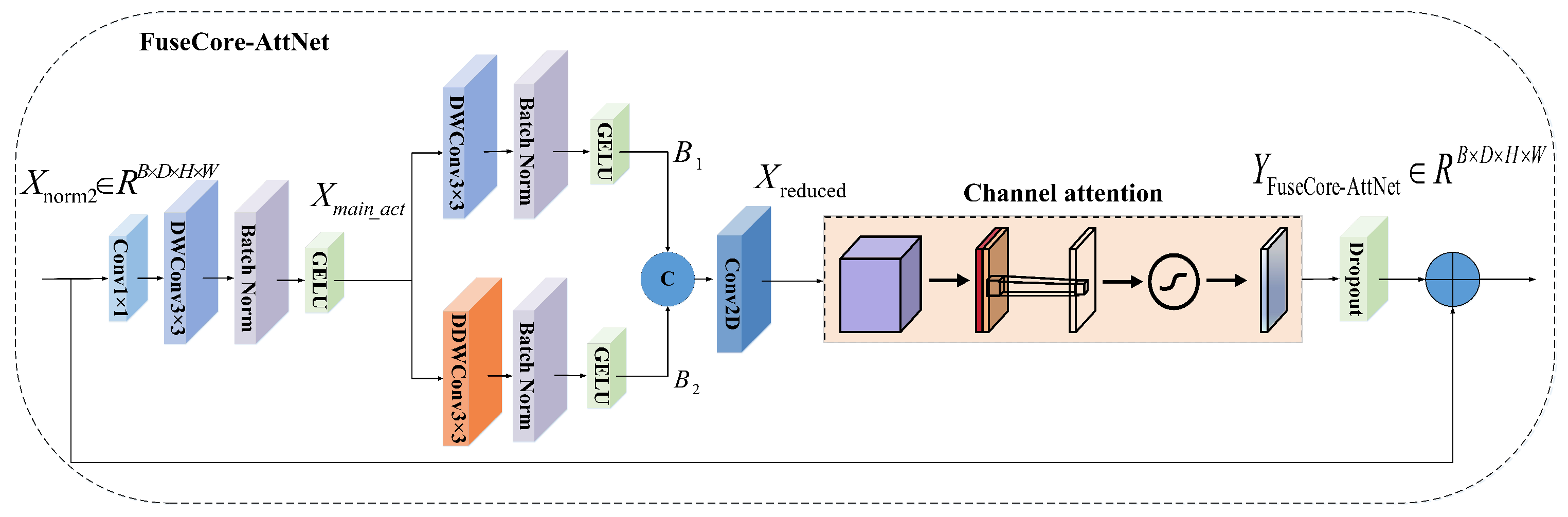
2.3. FuseCore-AttNet

In a standard VSS block, the feed-forward network (FFN) typically consists of two linear layers separated by a nonlinear activation function. This structure is highly efficient for processing flattened sequential data. However, for image features with two-dimensional spatial structures, purely linear layers fail to effectively capture the spatial correlations between neighboring pixels. To better adapt to the processing of image features and to introduce stronger local spatial awareness into the VSS block, we propose a convolutional feed-forward network, termed FuseCore-AttNet, to replace the standard FFN, as illustrated in Figure 2. The FuseCore-AttNet module takes a two-dimensional image feature tensor as the input. Its core idea is to replace the dimensionality expansion and reduction functions of linear layers with a series of convolutional operations. Moreover, it incorporates depth-wise separable convolutions and channel attention mechanisms to efficiently mix spatial features. Specifically, the input feature map $X_{norm2}$ is first passed through a 1 × 1 convolutional layer to increase the channel dimension. This operation expands the feature dimension from D to a hidden dimension $D_{hidden}=D\times mult$ without altering the spatial resolution. Then, a 3 × 3 depth-wise separable convolution followed by batch normalization is applied to the up-projected feature map $X_{exp}$. A GELU activation function is subsequently employed to introduce nonlinearity. This sequence forms the main pathway of the module, which is responsible for initial spatial feature mixing and nonlinear transformation.

$$\begin{array}{c}\hfill X_{\mathrm{main}\text{\_}\mathrm{act}}=GELU\left(\mathrm{BN}\left({\mathrm{DWConv}}_{3\times 3}\left(X_{\exp }\right)\right)\right)\end{array}$$

(10)

A key improvement of FuseCore-AttNet lies in the introduction of two parallel branches designed to enhance the extraction of spatial features. In Branch 1, a standard 3 × 3 depth-wise separable convolution is employed to focus on capturing spatial information within local neighborhoods.

$$\begin{array}{c}\hfill B_1=GELU\left(\mathrm{BN}\left({\mathrm{DWConv}}_{3\times 3}^{\mathrm{std}}\left(X_{\mathrm{main}\text{\_}\mathrm{act}}\right)\right)\right)\end{array}$$

(11)

For Branch 2, a 3 × 3 depth-wise separable convolution with dilation is used. By employing dilated convolutions, this branch can expand the receptive field and capture a larger spatial context without increasing the number of parameters or computational cost.

$$\begin{array}{c}\hfill B_2=GELU\left(\mathrm{BN}\left({\mathrm{DWConv}}_{3\times 3}^{\mathrm{dilated}}\left(X_{\mathrm{main}\text{\_}\mathrm{act}}\right)\right)\right)\end{array}$$

(12)

The outputs of these two parallel branches are then concatenated along the channel dimension and subsequently passed through a 1 × 1 convolutional layer for channel dimension reduction to obtain $X_{reduced}$. To further enhance the model’s channel-wise feature adaptivity, a squeeze-excitation (SE) attention module is applied to the reduced features. The SE module first compresses the spatial information of each channel into a scalar using global average pooling, then models the channel dependencies through two 1 × 1 convolutional layers (with ReLU activation and channel reduction in between), and finally generates channel-wise attention weights $W_{se}\in R^{B\times D\times 1\times 1}$ through a Sigmoid activation. These weights are element-wise multiplied with $X_{reduced}$, allowing for adaptive adjustment of the features along the channel dimension.

$$\begin{array}{c}\hfill {\mathbf{w}}_{se}=Sigmoid\left({Conv}_{1\times 1}^{se2}\left(ReLU\left({Conv}_{1\times 1}^{se1}\left(AdaptiveAvgPool2d\left(X_{\mathrm{reduced}}\right)\right)\right)\right)\right)\end{array}$$

(13)

$$\begin{array}{c}\hfill X_{\mathrm{main}\text{\_}\mathrm{act}}=X_{\mathrm{reduced}}\odot {\mathbf{w}}_{\mathrm{se}}\end{array}$$

(14)

Finally, Dropout is applied to the SE-weighted features $X_{s{e}_{s}caled}$ for regularization, and a residual connection is established between $X_{s{e}_{s}caled}$ and the original input features $X_{norm2}$, yielding the final output of the FuseCore-AttNet module.

$$\begin{array}{c}\hfill Y_{\mathrm{FuseCore}\text{-}\mathrm{AttNet}}=X_{\mathrm{norm}2}+DropPath\left(Dropout\left(X_{\mathrm{main}\text{\_}\mathrm{act}}\right)\right)\end{array}$$

(15)

2.4. Spatiotemporal Mixture-of-Experts Fusion Block

The core functionality of the spatiotemporal mixture-of-experts fusion block (STF-MoE block) lies in the fine-grained interaction and integration of multi-source and multitemporal features at each independent scale, as shown in Figure 3A. For each scale i, a dedicated fusion unit (stf-union) receives four corresponding input feature sets: $\left[E_{C_0}^i\right]$, $\left[\Delta E_{C_1,C_0}^i\right]$, $\left[E_{F_0}^i\right]$, and $\left[E_{C_1}^i\right]$. To fully exploit different types of information, we design both spatial expert and temporal expert modules. The spatial expert operates on the fine-resolution feature $E_{F_0}^i$ at time T0, aiming to enhance and refine the fine-grained spatial details contained in $F_0$. It achieves this through a 2D residual convolutional block integrated with a channel attention mechanism, which refines the spatial features of $E_{F_0}^i$. By enhancing discriminative spatial representations, the spatial expert provides a high-quality spatial foundation for predicting fine-resolution information at time T1.

$$\begin{array}{c}\hfill S{P}^i=SpatialExpert\left(E_{F_0}^i\right)\end{array}$$

(16)

The temporal expert operates on the coarse-resolution features $E_{C_0}^i$ and $E_{C_1}^i$ at time points T0 and T1, respectively, aiming to capture and model the change patterns and dynamic information across time. Features $E_{C_0}^i$ and $E_{C_1}^i$ are stacked along a new temporal dimension to form a $5D$ tensor, which is then fed into the temporal expert module. By analyzing this temporal cube, the temporal expert extracts change-sensitive features, providing crucial temporal context for predicting fine-resolution variations at T1.

$$\begin{array}{c}\hfill T{E}^i=TemporalExpert\left({\left[E_{C_0}^i,E_{C_1}^i\right]}_{\mathrm{stacked}}\right)\end{array}$$

(17)

To adaptively integrate the outputs of the spatial and temporal experts with the original fine-resolution information at T0, the model generates gating weights based on $E_{F_0}^i$. Specifically, $E_{F_0}^i$ is passed through a 1 × 1 convolutional layer followed by a Sigmoid activation to produce the spatial gate $G_S^i$ and temporal gate $G_T^i$. These two gates dynamically modulate the contributions of the expert outputs. The enhanced feature E is obtained by combining the original feature F with the gated expert outputs, where ⊙ denotes element-wise multiplication.

$$\begin{array}{c}\hfill \left(G_S^i,G_T^i\right)=\sigma \left(Conv1x1\left(E_{F_0}^i\right)\right)(\mathrm{split}\mathrm{into}\mathrm{two}\mathrm{halves})\end{array}$$

(18)

$$\begin{array}{c}\hfill X_{\mathrm{enhanced}}^i=E_{F_0}^i+G_S^i\odot S{P}^i+G_T^i\odot T{E}^i\end{array}$$

(19)

Subsequently, the normalized output $X_{norm}^i$, together with $E_{C_0}^i$, $\Delta E_{C_1,C_0}^i$, and $E_{C_1}^i$, is fed into the stf-union. The stf-union first computes the correlation feature $co{r}^i$ between $X_{norm}^i$ and $E_{C_0}^i$, modeling the correspondence between the coarse- and fine-resolution features at time T0.

$$\begin{array}{c}\hfill {cor}^i=SiLU\left(Conv\left(X_{\mathrm{norm}}^i-E_{C_0}^i\right)\right)\end{array}$$

(20)

Then, $co{r}^i$ is used to perform both change-based prediction and T1 coarse-resolution-based prediction. For change-based prediction, $co{r}^i$ is used to modulate the coarse-resolution change feature $\Delta E_{C_1,C_0}^i$ to predict the fine-resolution change increment ${\Delta }_{pred}^i$, resulting in an initial prediction $P_1^i$. For the T1 coarse-resolution-based prediction, $co{r}^i$ is used to map the T1 coarse-resolution feature $E_{C_1}^i$ into the fine-resolution space, yielding the final prediction $P_2^i$.

$$\begin{array}{c}\hfill {\Delta }_{\mathrm{pred}}^i=ConvDiff\left(\Delta E_{C_1,C_0}^i\right)\odot {cor}^i\end{array}$$

(21)

$$\begin{array}{c}\hfill P_1^i=X_{\mathrm{norm}}^i+{\Delta }_{\mathrm{pred}.}^i\end{array}$$

(22)

$$\begin{array}{c}\hfill P_2^i=E_{C_1}^i\odot {\mathrm{cor}}^i\end{array}$$

(23)

Finally, the two prediction results are combined and further refined using channel attention to obtain $P^i$. The refined output is then fused with the original features $E_{F_0}^i$ and $E_{C_1}^i$ through a residual connection, resulting in the final fused feature $Y^i$.

$$\begin{array}{c}\hfill Y^i=\mathrm{ChannelAttentionBlock}\left(P^i\right)+E_{F_0}^i+E_{C_1}^i\end{array}$$

(24)

2.5. Temporal Expert

One of the key challenges in spatiotemporal fusion lies in effectively capturing and leveraging changes across different time points, particularly under resolution mismatch. To specifically model the dynamic changes from time T0 to T1 at the coarse resolution, we design a temporal expert, as illustrated in Figure 3B. This expert operates on the T0 and T1 coarse-resolution features $E_{C_0}^i$ and $E_{C_1}^i$ at the same scale i, aiming to extract feature representations that are sensitive to temporal variations. The temporal expert incorporates 3D convolutional layers, batch normalization, and a nonlinear activation function (SiLU), with information propagated through a residual connection structure. The 3D convolutions enable simultaneous feature extraction and fusion across both temporal and spatial dimensions, thereby capturing interactions between temporal changes and spatial patterns. To further enhance the model’s sensitivity to the importance of features at different time steps, we embed a temporal SE (squeeze-and-excitation) attention mechanism within the temporal expert. Unlike the standard SE attention that performs compression and excitation along the channel dimension, the temporal SE attention focuses specifically on the temporal dimension. It first applies a pooling operation across the spatial dimensions of ($H_i^{\prime }\times W_i^{\prime }$) to compress the spatial information of each channel at each time step into a scalar, forming a tensor $X_{\mathrm{temporal}}^i$ with shape $R^{B\times D_i\times 2\times 1\times 1}$. This tensor is then fed into a lightweight $3D$ convolutional network to learn importance weights for different combinations of time steps and channels. Finally, a Sigmoid activation is applied to constrain the weights between 0 and 1, resulting in the temporal attention weight tensor $W_{temporal}$.

$$\begin{array}{c}\hfill {\mathbf{W}}_{\mathrm{temporal}}=Sigmoid\left({Conv}_{1\times 1\times 1}^{se2}\left(ReLU\left({Conv}_{1\times 1\times 1}^{se1}\left(AdaptiveAvgPool3\mathrm{d}\left(X_{\mathrm{temporal}}^i\right)\right)\right)\right)\right)\end{array}$$

(25)

These temporal attention weights are applied element-wise to the feature maps produced by the main 3D convolutional layers, adaptively modulating the contributions of features at different time steps.

$$\begin{array}{c}\hfill X_{\mathrm{temporal}}^{\prime }=3\mathrm{DConvBlock}\left(X_{\mathrm{temporal}}^i\right)\end{array}$$

(26)

$$\begin{array}{c}\hfill X_{\mathrm{temporal}}^{″}=X_{\mathrm{temporal}}^{\prime }\odot {\mathbf{W}}_{\mathrm{temporal}}\end{array}$$

(27)

Finally, the temporal expert outputs the time-aware feature $T{E}^i$ for the given scale through a residual connection.

$$\begin{array}{c}\hfill T{E}^i=\mathrm{ProcessTimeDimension}\left(\mathrm{ResidualConnection}\left(X_{\mathrm{temporal}}^i,X_{\mathrm{temporal}}^{″}\right)\right)\end{array}$$

(28)

2.6. Spatial Expert

In multi-scale spatiotemporal fusion tasks, accurately capturing and preserving spatial details in fine-resolution imagery is critical. To enhance the model’s ability to process spatial information from the T0 fine-resolution image $F_0$, we design a spatial expert for each scale, as illustrated in Figure 3C. This expert takes the fine-resolution feature $E_{F_0}^i$ at the corresponding scale of T0 as input, aiming to enhance discriminative spatial features and texture details through refined spatial processing. Internally, it consists of two 3 × 3 convolutional layers, batch normalization, a nonlinear activation function (SiLU), and a channel attention module for adaptive weighting of channel-wise features. The input feature C$E_{F_0}^i$ first passes through the first 3 × 3 convolutional layer, followed by batch normalization and SiLU activation.

$$\begin{array}{c}\hfill X_1=SiLU\left({\mathrm{BN}}_1\left({Conv}_{3\times 3}^1\left(E_{F0}^i\right)\right)\right)\end{array}$$

(29)

The activated feature $X_1$ is passed through a second 3 × 3 convolutional layer followed by batch normalization to produce $X_2$. To enable the model to adaptively focus on the importance of different channels, we incorporate a channel attention mechanism into the main pathway. The channel attention module takes the feature map as input and first applies global average pooling and global max pooling to compress the spatial information of each channel into two scalars, which are then summed. This channel descriptor vector is then passed through a lightweight network—composed of two 1 × 1 convolutional layers with an intermediate SiLU nonlinear activation—to capture complex inter-channel dependencies. Finally, a Sigmoid activation function is applied to generate the channel-wise weights $W_{CA}$, each ranging from 0 to 1. Here, $Con{v}_{1\times 1}^{se1}$ performs channel reduction, while $Con{v}_{1\times 1}^{se2}$ performs channel expansion.

$$\begin{array}{c}\hfill {\mathbf{W}}_{CA}=\sigma \left({Conv}_{1\times 1}^{se2}\left(SiLU\left({Conv}_{1\times 1}^{se1}\left(AvgPool\left(X_2\right)+MaxPool\left(X_2\right)\right)\right)\right)\right)\end{array}$$

(30)

The learned channel weights $W_{CA}$ are applied to the feature map $X_2$ via element-wise multiplication to enhance the features of important channels, resulting in feature map $X_{CA\_scaled}$. Finally, to maintain smooth information flow and facilitate training, the attention-adjusted feature map $X_{CA\_scaled}$ is combined with the original input feature $E_{F_0}^i$ through a residual connection. The resulting tensor is then passed through a final SiLU activation layer to produce the output $S{P}^i$ of the spatial expert at this scale.

$$\begin{array}{c}\hfill X_{CA\_\mathrm{scaled}}=X_2\odot {\mathbf{W}}_{CA}\end{array}$$

(31)

$$\begin{array}{c}\hfill X_{\mathrm{residual}}=E_{F0}^i+X_{CA\_\mathrm{scaled}}\end{array}$$

(32)

$$\begin{array}{c}\hfill S{P}^i=SiLU\left(X_{\mathrm{residual}}\right)\end{array}$$

(33)

2.7. Loss Function

To effectively train the proposed Mamba-STFM model and enable it to generate synthetic images $\widehat{F_1}$ that closely match the real high-resolution images in both pixel values and spatial structure, we employ a composite loss function $\mathcal{L}$ that combines pixel-level error and structural similarity. The primary optimization objective is to ensure that the pixel values of the predicted image $\widehat{F_1}$ closely approximate those of the ground truth image $F_1$. We adopt the mean squared error (MSE) as the pixel-level loss component ${\mathcal{L}}_{MSE}$. The $MSE$ loss measures the average squared differences between the predicted output and the ground truth, effectively guiding model convergence and penalizing large pixel-wise deviations. Here, P and $GT$ denote the predicted and ground truth images, respectively; C, H, and W represent the number of channels, height, and width; and $P_{c,i,j}$ and $G{T}_{c,i,j}$ indicate their pixel values at channel c, row i, and column j.

$$\begin{array}{c}\hfill {\mathcal{L}}_{MSE}(P,GT)={\displaystyle \frac{1}{C·H·W}}\sum _{c=1}^C\sum _{i=1}^H\sum _{j=1}^W{\left(P_{c,i,j}-G{T}_{c,i,j}\right)}^2\end{array}$$

(34)

Relying solely on pixel-level loss often fails to adequately capture the spatial structural information of images, which may result in blurred edges or distorted textures in the synthesized images. To guide the model in generating outputs that are structurally closer to real images, we introduce a loss term ${\mathcal{L}}_{\mathcal{SSIM}}$ based on the structural similarity index measure ($SSIM$). $SSIM$ is a widely used metric for evaluating image quality and similarity, which assesses luminance, contrast, and structural information. Its values range from 0 to 1, with higher values indicating greater similarity between two images. We convert $SSIM$ into a loss function by minimizing its complement, thereby maximizing structural similarity during training.

$$\begin{array}{c}\hfill {\mathcal{L}}_{SSIM}\left(P,GT\right)=1-SSIM\left(P,GT\right)\end{array}$$

(35)

The final loss function $\mathcal{L}$ used to train the Mamba-STFM model is formulated as a linear combination of the $MSE$ loss and the $SSIM$-based structural loss.

$$\begin{array}{c}\hfill \mathcal{L}={\lambda }_{MSE}{\mathcal{L}}_{MSE}\left({\widehat{Y}}_{t_2}^{\mathrm{fine}},Y_{t_2}^{\mathrm{fine}}\right)+{\lambda }_{SSIM}{\mathcal{L}}_{SSIM}\left({\widehat{Y}}_{t_2}^{\mathrm{fine}},Y_{t_2}^{\mathrm{fine}}\right)\end{array}$$

(36)

${\lambda }_{MSE}$ and ${\mathcal{L}}_{MSE}$ are non-negative weighting coefficients used to balance the contributions of the two loss components to the overall optimization objective. The model parameters are updated using standard gradient descent and backpropagation algorithms to minimize the combined loss function $\mathcal{L}$.

3. Experiments

3.1. Study Area and Datasets

In the field of spatiotemporal fusion of remote sensing imagery, data availability is of critical importance. Among available datasets, the widely recognized Coleambally Irrigation Area (CIA) and Lower Gwydir Catchment (LGC) serve as foundational benchmarks for evaluating the performance of fusion algorithms. These datasets are valuable because they offer multiband remote sensing observation sequences across multiple time points, providing a standardized platform for researchers to assess the accuracy and robustness of spatiotemporal fusion algorithms in capturing and reconstructing various surface dynamics—ranging from gradual phenological changes to abrupt environmental events. Within the framework of this study, we employ these two datasets to conduct a detailed comparative evaluation of the proposed Mamba-STFM model against representative existing methods in terms of fusion performance.

Specifically, the CIA dataset [51] was designed to capture seasonal phenological cycles in agricultural regions. The dataset contains 17 carefully selected pairs of cloud-free Landsat and MODIS images, each covering an area of 2040 × 1720 pixels. The time series spans from 7 October 2001 to 3 May 2002, capturing surface conditions during that period. Geographically, the dataset corresponds to the Coleambally Irrigation Area in southern New South Wales, Australia.

In contrast to the CIA dataset, the LGC dataset [52] focuses on detecting and modeling rapid and drastic surface changes, with flood events serving as a typical example. This dataset comprises 14 pairs of cloud-free Landsat and MODIS images, with a larger spatial coverage of 3200 × 2720 pixels. It captures surface changes that occurred between 16 April 2004 and 3 April 2005. The study area is located in the Lower Gwydir Catchment in Northern New South Wales, Australia. Notably, during the time span of this dataset, a major flood event occurred in mid-December 2004, inundating approximately 44% of the area. This provides a realistic and challenging test scenario for evaluating algorithm performance under sudden environmental changes.

3.2. Experimental Details

To evaluate the performance of the proposed Mamba-STFM model, we conducted comparative experiments on the CIA and LGC datasets against seven representative spatiotemporal fusion methods. These methods include STARFM [15] and ESTARFM [16] (two classical traditional approaches), as well as GANSTFM [42], EDCSTFN [20], Swin-STFM [45], ECPW-STFN [53], and STFDiff [54] (all deep learning-based models). Each of these deep learning models has distinct characteristics: GANSTFM employs a conditional generative adversarial network, EDCSTFN is a deep model based on convolutional neural networks, Swin-STFM is built on the Transformer architecture, STFDiff performs fusion using a diffusion model, and ECPW-STFN is a wavelet-based pairing network.

Our experimental design focuses on four core components, all conducted on the publicly available CIA and LGC datasets. Prior to formal evaluation, the datasets were partitioned into training and testing sets. For the CIA dataset, the training period spans from 8 October 2001 to 11 April 2002 and the testing period from April 18 to 4 May 2002, with the prediction target date set as 27 April 2002. For the LGC dataset, the training set includes data from 16 April to 25 October 2004 and 13 January to 3 April 2005. The testing set consists of data from 26 November to 28 December 2004, with the prediction target date being 12 December 2004. Once the data preparation was complete, we carried out the following experiments: (1) quantitative performance comparisons of various fusion methods on the test sets; (2) qualitative analysis of the fused image details produced by each method; (3) ablation studies to evaluate the contribution of key components within the Mamba-STFM model; and (4) comparative evaluation of the classification performance of different models using the K-means clustering algorithm.

The proposed Mamba-STFM fusion method was implemented using Python 3.9.21 and PyTorch 1.13.1. The encoder comprises four stages, with the number of VSS-FCAN blocks set to two, two, nine, and two for each respective stage. The dimensionality parameters for downsampling are set to 96, 192, 384, and 768, respectively. The spatiotemporal fusion module operates across four scale levels, each containing one STF-Union unit. The MambaDecoder in the decoder stage has depths configured as one, one, one, and one.

The model is trained using the Adaptive Moment Estimation (ADAM) optimizer with an initial learning rate of $1\times {10}^{-4}$, a batch size of 4, a patch size of 256, and for 50 training epochs. A dynamic learning rate adjustment strategy is employed: if the training loss does not decrease for four consecutive epochs, the learning rate is automatically reduced by a factor of 0.5. Sensitivity analysis shows that the model is relatively robust to batch size variations, and its performance remains stable across batch sizes ranging from 2 to 16. The training process does not exhibit any oscillation or divergence, and the loss curves demonstrate smooth and consistent convergence.

The parameter settings for other spatiotemporal fusion methods follow the original authors’ configurations to ensure fair comparison. All baseline models were retrained using the same training, validation, and test splits as Mamba-STFM. All experiments were conducted on a server equipped with an NVIDIA RTX 3090 GPU (24 GB), an Intel Platinum 8362 CPU, and 45 GB of RAM.

3.3. Assessment of Metrics

To comprehensively evaluate the performance of the fused images, five key metrics are employed in this study: root mean square error (RMSE), structural similarity index (SSIM), universal image quality index (UIQI), correlation coefficient (CC), and Erreur Relative Globale Adimensionnelle de Synthèse (ERGAS). These metrics assess fusion quality from multiple perspectives: RMSE quantifies pixel-wise deviations, where lower values indicate higher accuracy; SSIM evaluates structural fidelity, with values ranging from 0 to 1, where values closer to 1 denote greater structural similarity; UIQI assesses image quality by analyzing distortion in correlation, luminance, and contrast, ranging from −1 to 1, with 1 indicating perfect statistical consistency; CC reflects the strength of linear correlation between images, also ranging from −1 to 1, where 1 indicates perfect positive correlation; ERGAS offers a band-wise global relative error assessment, where lower values signify better overall fusion performance. Details of each metric are provided in

Table 1. Image quality evaluation metrics and formula explanation.

Metric	Formula	Symbol Explanation
RMSE	$\mathrm{RMSE}=\sqrt{{\displaystyle \frac{1}{N}}{\sum }_{i=1}^N{(a_i-b_i)}^2}$	N: Total number of pixels $a_i$: The i-th pixel in the reference image $b_i$: The i-th pixel in the image to be evaluated
SSIM	$\mathrm{SSIM}={\displaystyle \frac{(2m_a{m}_b+C_1)(2c_{ab}+C_2)}{(m_a^2+m_b^2+C_1)(v_a+v_b+C_2)}}$	$m_a,m_b$: Local mean of the two images $v_a,v_b$: Local variance of the two images $c_{ab}$: Local covariance of the two images $C_1,C_2$: Stability constants
UIQI	$Q={\displaystyle \frac{4c_{ab}{m}_a{m}_b}{(v_a+v_b)(m_a^2+m_b^2)}}$	Same symbols as SSIM: $m_a,m_b$: Local mean $v_a,v_b$: Local variance $c_{ab}$: Local covariance
CC	$\mathrm{CC}={\displaystyle \frac{{\sum }_{i=1}^N(a_i-m_a)(b_i-m_b)}{\sqrt{{\sum }_{i=1}^N{(a_i-m_a)}^2}\sqrt{{\sum }_{i=1}^N{(b_i-m_b)}^2}}}$	N: Number of pixels $a_i,b_i$: Pixel values in the two images $m_a={\displaystyle \frac{1}{N}}{\sum }_{i=1}^N{a}_i$, $m_b={\displaystyle \frac{1}{N}}{\sum }_{i=1}^N{b}_i$: Global mean of the images
ERGAS	$\mathrm{ERGAS}=100·{\displaystyle \frac{h_L}{h_H}}\sqrt{{\displaystyle \frac{1}{B}}{\sum }_{k=1}^B{\left({\displaystyle \frac{R_k}{M_k}}\right)}^2}$	B: Number of bands $R_k$: RMSE of the k-th band $M_k$: Mean value of the reference image for the k-th band $h_L,h_H$: Pixel size of low/high resolution images

.

4. Results

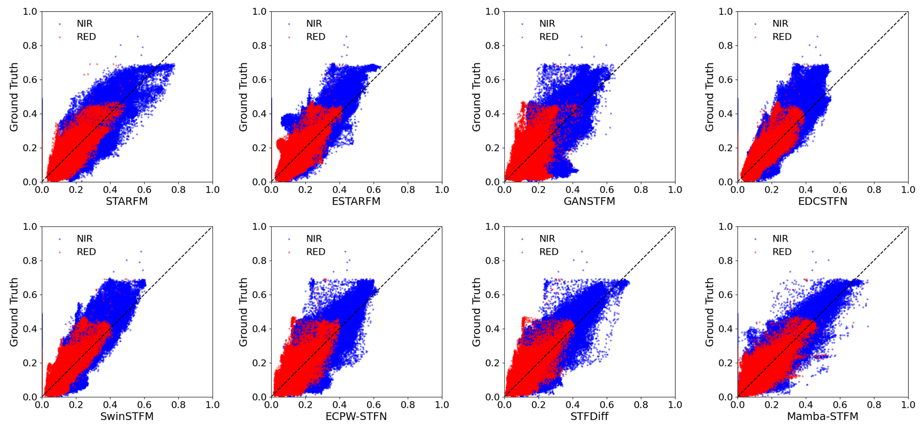
4.1. Comparison of Various Fusion Methods on the CIA Dataset

4.1.1. Quantitative Comparison

Based on the CIA dataset, we conducted a comprehensive quantitative evaluation of eight spatiotemporal fusion models—STARFM, ESTARFM, GANSTFM, EDCSTFN, SwinSTFM, ECPW-STFN, STFDiff, and Mamba-STFM—using key metrics widely adopted in the remote sensing image fusion field, including RMSE, SSIM, UIQI, CC, and ERGAS. The evaluation results in

Table 2. Quantitative comparison of various fusion methods on the CIA dataset. The black bold font represents the best value.

Metrics	Band	STARFM	ESTARFM	GANSTFM	EDCSTFN	SwinSTFM	ECPW-STFN	STFDiff	Mamba-STFM
RMSE	1	0.0174	0.0136	0.0139	0.0126	0.0112	0.0125	0.0093	0.0086
	2	0.0236	0.0195	0.0202	0.0161	0.0148	0.0137	0.0128	0.0115
	3	0.0333	0.0306	0.0313	0.0255	0.0217	0.0152	0.0197	0.0169
	4	0.0538	0.0515	0.0547	0.0452	0.0299	0.0261	0.0263	0.0256
	5	0.0560	0.0537	0.0563	0.0484	0.0363	0.0349	0.0335	0.0311
	6	0.0544	0.0482	0.0552	0.0433	0.0306	0.0285	0.0288	0.0277
SSIM	1	0.8756	0.9079	0.9037	0.9151	0.9387	0.9326	0.9424	0.9515
	2	0.8674	0.8869	0.9093	0.9293	0.9254	0.9311	0.9385	0.9363
	3	0.8220	0.8538	0.8405	0.8634	0.8845	0.8904	0.8901	0.8976
	4	0.7516	0.7825	0.7350	0.8419	0.8216	0.8455	0.8468	0.8640
	5	0.7936	0.7847	0.7891	0.7853	0.7725	0.7893	0.7914	0.8092
	6	0.7717	0.7806	0.7822	0.7911	0.7917	0.7972	0.8116	0.8184
UIQI	1	0.7227	0.7744	0.7983	0.8216	0.8362	0.8361	0.8355	0.8863
	2	0.7157	0.7830	0.7371	0.8508	0.8656	0.8881	0.8816	0.9162
	3	0.8056	0.8231	0.8062	0.8619	0.8728	0.8908	0.9043	0.9206
	4	0.8228	0.8360	0.8419	0.9026	0.9168	0.9249	0.9222	0.9435
	5	0.8531	0.8586	0.8504	0.9212	0.9207	0.9311	0.9365	0.9430
	6	0.8604	0.8728	0.8849	0.9255	0.9215	0.9357	0.9331	0.9369
CC	1	0.7305	0.7887	0.7636	0.8251	0.8463	0.8656	0.8739	0.8952
	2	0.7554	0.7931	0.7760	0.8439	0.8723	0.9081	0.9058	0.9195
	3	0.7791	0.8296	0.8394	0.8510	0.8785	0.8907	0.9032	0.9226
	4	0.8336	0.8387	0.8532	0.9157	0.9188	0.9258	0.9217	0.9440
	5	0.8529	0.8595	0.8648	0.9215	0.9209	0.9344	0.9331	0.9471
	6	0.8514	0.8732	0.8917	0.9184	0.9215	0.9358	0.9386	0.9378
ERGAS	-	1.7086	1.5995	1.6057	1.2590	1.0658	0.9633	0.9149	0.8615

indicate that the Mamba-STFM model achieves state-of-the-art performance. As a global indicator of overall spectral and spatial quality (where lower values indicate better performance), Mamba-STFM yielded the lowest ERGAS value of 0.8615. This represents a reduction of 0.0534 compared with the second best model, STFDiff (0.9149), and a substantial decrease of 0.8471 compared with the weakest traditional model, STARFM (1.7086), highlighting a significant overall improvement. Furthermore, Mamba-STFM consistently demonstrated superior performance across individual spectral bands, achieving the lowest RMSE and the highest SSIM, UIQI, and CC values in the vast majority of bands. Notably, in terms of the UIQI metric, which evaluates overall image quality, Mamba-STFM attained the highest values across all six spectral bands, underscoring its strong capability in preserving image fidelity. These comprehensive quantitative results strongly support the superior performance and leading position of the Mamba-STFM model in spatiotemporal image fusion on this dataset.

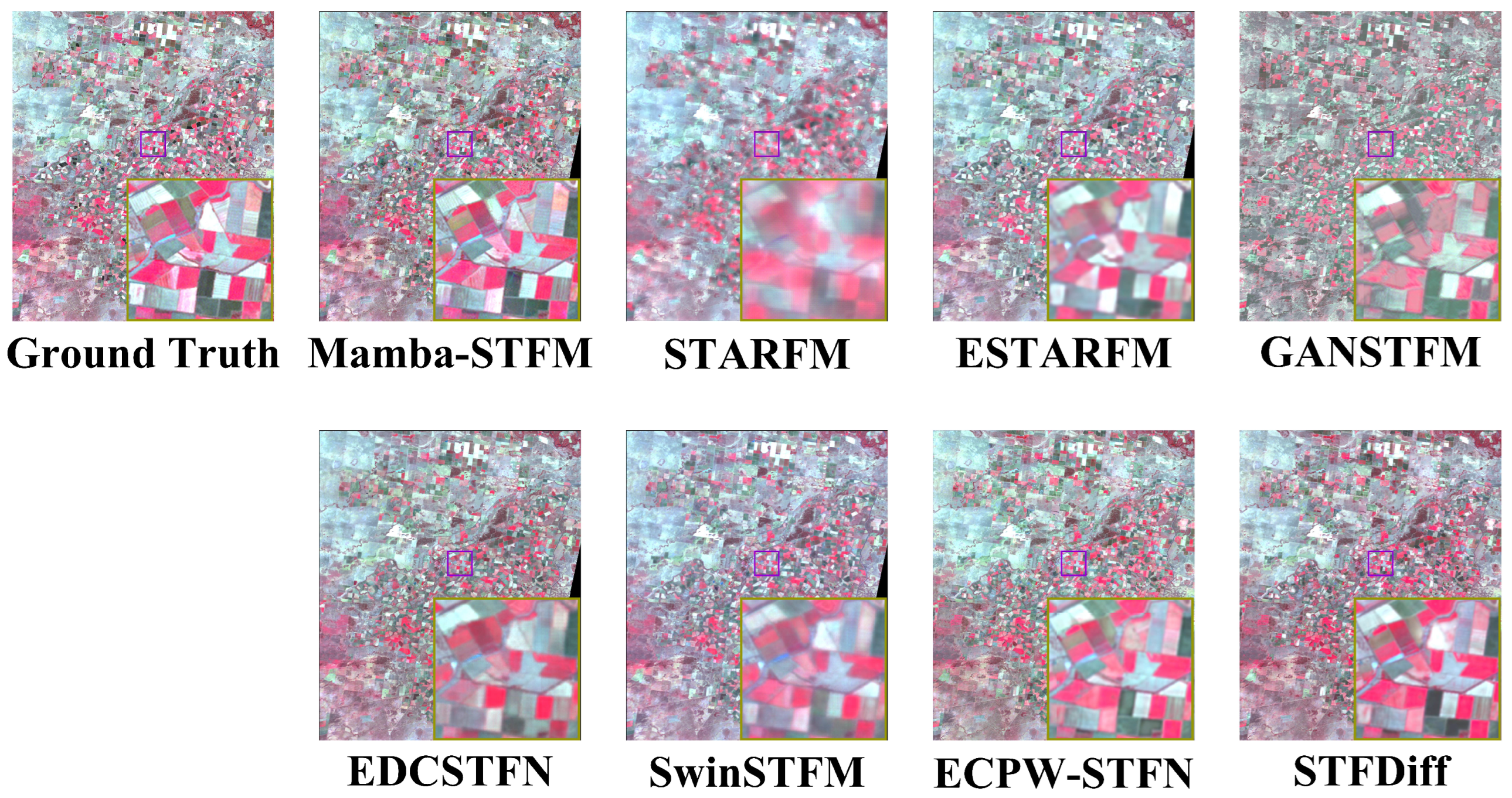
4.1.2. Detail Comparison

To provide a more intuitive assessment of the fusion performance of different methods, we compared the details of various fusion products on the CIA dataset. As shown in Figure 4 (27 April 2002, CIA dataset agricultural area), significant differences are observed among the methods in terms of micro-texture and field boundary restoration: The STARFM fusion results are overly smoothed, with blurred small-scale field boundaries and discontinuous spectral transitions; ESTARFM insufficiently reconstructs fragmented structures, with noticeable edge diffusion. While GANSTFM introduces some texture details, it is accompanied by artifact stripes and spectral distortions; EDCSTFN and ECPW-STFN show limited improvement in overall texture, with residual noise interference and block effects; SwinSTFM results exhibit a noticeable grid-like block structure, with unclear distribution of multi-scale objects; STFDiff has limited high-frequency detail restoration, with significant boundary noise. In contrast, Mamba-STFM performs best in maintaining field geometry and color contrast, accurately reconstructing small-scale vegetation block distributions, preserving sharp boundaries, minimizing spectral bias, and demonstrating the highest structural similarity and optimal fusion details.

As shown in Figure 5 (27 April 2002, CIA dataset), there are significant differences in the pixel-level RMSE distributions of the various methods: GANSTFM produces large “high-error areas” at field boundaries and mixed crop interfaces, with pixel RMSE frequently exceeding 0.06; STARFM and ESTARFM reduce errors in homogeneous areas but are accompanied by scattered high-error patches (RMSE > 0.05), corresponding to pseudo-textures; EDCSTFN and ECPW-STFN suppress overall errors compared with STARFM but still leave relatively high RMSEs in localized regions due to blocky artifacts. While SwinSTFM and STFDiff better capture fine structures and reduce large-scale hotspots, they show increased errors at boundaries, with RMSE distribution tails extending; in contrast, Mamba-STFM exhibits the most uniform error field, with the majority of pixel RMSE values below 0.05 and minimal high errors, providing strong evidence of its ability to achieve optimal fusion with minimal spectral distortion when reconstructing both homogeneous and heterogeneous agricultural features.

4.2. Comparison of Various Fusion Methods on the LGC Dataset

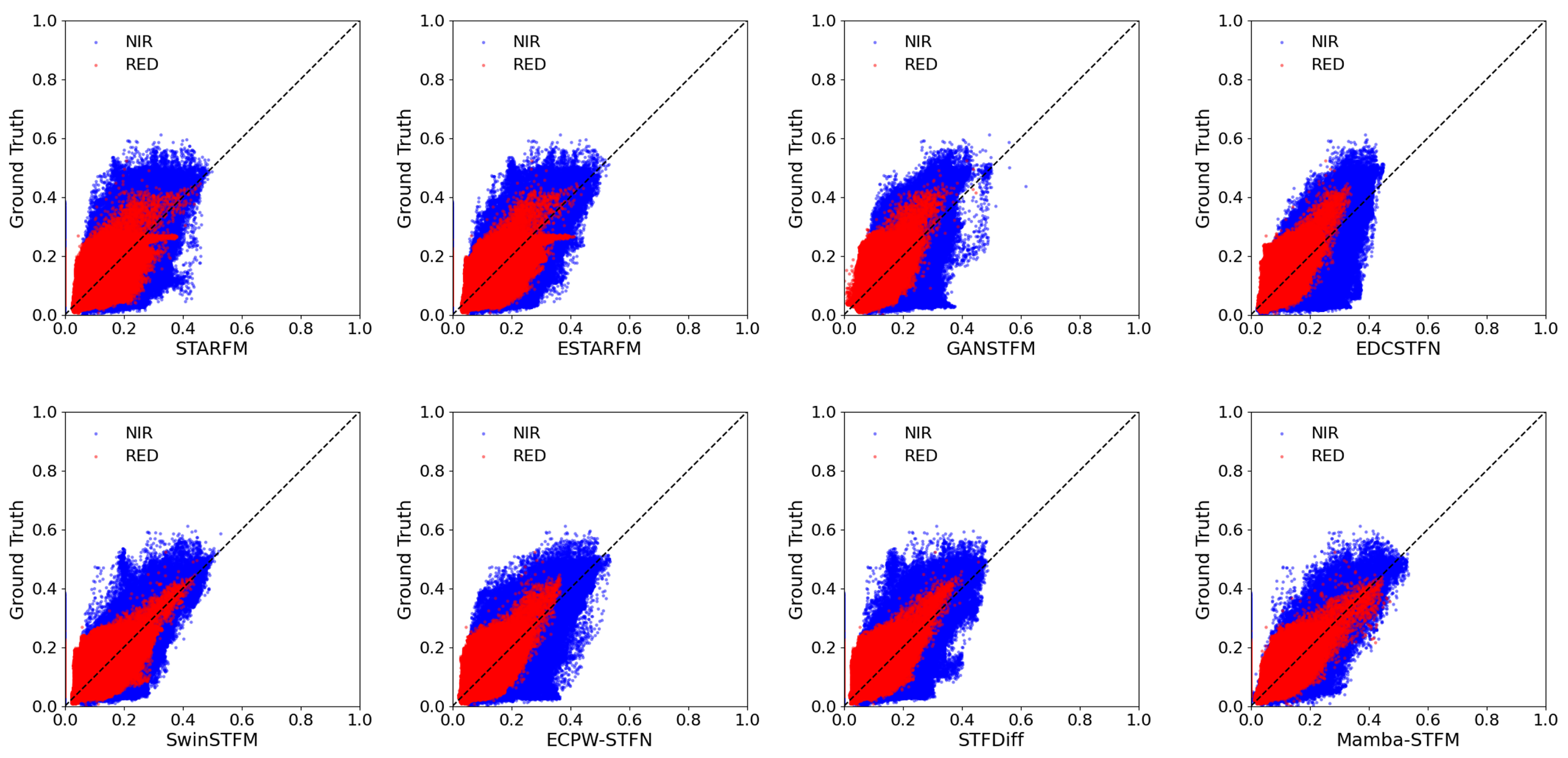
4.2.1. Quantitative Comparison

A quantitative evaluation on the LGC dataset also compared eight spatiotemporal fusion models, including Mamba-STFM. The analysis results, as shown in

Table 3. Quantitative comparison of various fusion methods on the LGC dataset, with the best values in bold.

Metrics	Band	STARFM	ESTARFM	GANSTFM	EDCSTFN	SwinSTFM	ECPW-STFN	STFDiff	Mamba-STFM
RMSE	1	0.0146	0.0139	0.0155	0.0134	0.0122	0.0117	0.0105	0.0098
	2	0.0189	0.0185	0.0212	0.0196	0.0178	0.0145	0.0149	0.0127
	3	0.0269	0.0268	0.0264	0.0255	0.0229	0.0214	0.0197	0.0165
	4	0.0399	0.0395	0.0410	0.0381	0.0294	0.0288	0.0281	0.0234
	5	0.0541	0.0552	0.0538	0.0545	0.0435	0.0414	0.0427	0.0335
	6	0.0427	0.0424	0.0399	0.0406	0.0319	0.0299	0.0304	0.0257
SSIM	1	0.9305	0.9381	0.9261	0.9327	0.9397	0.9472	0.9450	0.9494
	2	0.8976	0.9024	0.9042	0.9187	0.9060	0.9114	0.9161	0.9246
	3	0.8577	0.8582	0.8718	0.8712	0.8736	0.8819	0.8812	0.8958
	4	0.7343	0.7672	0.7927	0.8129	0.8159	0.8142	0.8063	0.8395
	5	0.6114	0.6314	0.6353	0.6517	0.7039	0.7197	0.7260	0.7569
	6	0.6676	0.6792	0.6923	0.7160	0.7604	0.7646	0.7728	0.8026
UIQI	1	0.6013	0.6792	0.6517	0.6983	0.7765	0.7855	0.7962	0.8775
	2	0.6744	0.7153	0.6716	0.7579	0.7727	0.7750	0.7894	0.8826
	3	0.6948	0.7298	0.6970	0.7544	0.7693	0.7784	0.7751	0.8832
	4	0.7439	0.7801	0.7175	0.7973	0.8771	0.8913	0.8806	0.9244
	5	0.7422	0.8086	0.7652	0.8065	0.8683	0.8840	0.8752	0.9230
	6	0.7519	0.8060	0.7633	0.8073	0.8698	0.8699	0.8814	0.9148
CC	1	0.6831	0.7018	0.6192	0.7236	0.7825	0.8144	0.8039	0.8845
	2	0.7188	0.7511	0.6317	0.6964	0.7757	0.7829	0.7875	0.8873
	3	0.7062	0.7455	0.6510	0.6877	0.7719	0.7753	0.7803	0.8868
	4	0.7652	0.7942	0.7478	0.7973	0.8827	0.8966	0.9028	0.9266
	5	0.7913	0.8056	0.7892	0.8065	0.8715	0.8802	0.8896	0.9247
	6	0.8044	0.8032	0.7831	0.8073	0.8720	0.8911	0.8952	0.9174
ERGAS	-	1.9042	1.8872	2.1317	1.9688	1.6179	1.4413	1.4260	1.2472

, provide a clear performance overview: the Mamba-STFM model leads comprehensively among all evaluated models, ranking first across all performance metrics. Specifically, Mamba-STFM achieved the lowest RMSE values across all six spectral bands in the reconstruction error dimension; simultaneously, in terms of image quality, structural similarity, and correlation, as reflected by SSIM, UIQI, and CC, it also set new records for the highest values in each band. Particularly crucial is the ERGAS metric, which provides a global performance evaluation (where lower values indicate better performance). Mamba-STFM achieved the lowest score of 1.2472, securing its outstanding position. This result not only outperforms the second best STFDiff model (1.4260) by 0.1788 points but also shows a significant improvement of 0.8845 compared with the lowest-performing GANSTFM model (2.1317). These overwhelming quantitative results collectively establish Mamba-STFM’s state-of-the-art performance on the LGC dataset.

4.2.2. Detail Comparison

Figure 6 presents a comparison of the details after spatiotemporal fusion of the flood area on the LGC dataset from December 12, 2004, using various fusion methods. Significant differences are observed in the sharpness of water boundaries and the reproduction of details at object conflicts. The STARFM results generally exhibit over-smoothing, with blurred flood edges and unnatural spectral jumps at the land–water interface; ESTARFM underestimates the spatial expansion of newly formed water channels and flooded patches, resulting in a contracted water body range. While GANSTFM enhances the texture of localized water bodies, it introduces strip artifacts and spectral shifts, which hinder accurate flood area identification; EDCSTFN and ECPW-STFN show slight improvements in detail recovery over STARFM, but residual noise and blocky artifacts still impede the resolution of small-scale tributary networks; SwinSTFM exhibits noticeable grid-like textures, with discontinuous breaks in the flood distribution; STFDiff, while introducing some high-frequency information, still shows a blurred land–water boundary and spectral deviations. In contrast, Mamba-STFM best preserves the flood geometry and spatial details, clearly depicting the floodplain and small-scale tributary systems, while achieving smooth transitions and spectral consistency at the land–water interface. It also exhibits the highest overall structural similarity index.

Figure 7 presents the pixel-level RMSE error distribution of fusion results from various spatiotemporal models on the LGC dataset from 12 December 2004 (representing a land cover change scenario caused by flooding). The color intensity in the error map visually reflects the difference between the fusion results and the true image. As seen in the figure, models such as STARFM, ESTARFM, GANSTFM, EDCSTFN, SwinSTFM, and ECPW-STFN generally exhibit high fusion errors in regions with significant land cover changes (such as the darker areas in the lower left and center of the image). In contrast, the STFDiff model shows reduced errors in these change areas, while the error map generated by the Mamba-STFM model has the lightest overall color and the most uniform distribution, particularly with significantly lower errors in the flood area compared with all other models. This indicates that the Mamba-STFM model demonstrates the best performance in handling the complex land cover changes represented by the LGC dataset (such as flooding). It more effectively captures and predicts surface changes, producing more precise fusion results and significantly reducing pixel-level errors.

4.3. Comparison of the Efficiency of Various Spatiotemporal Fusion Methods

To evaluate the performance of various deep learning-based spatiotemporal fusion models for remote sensing images, this study focuses on comparing the computational efficiency and fusion accuracy of six models based on different network architectures. The evaluation metrics include computational complexity (G FLOPs), number of parameters (M parameters), average inference time (ms), max memory usage (MB), and the average correlation coefficient (CC) for each channel across two different datasets. All model evaluations were conducted on a server equipped with an RTX 3090 GPU, with the input image size fixed at 256 × 256 and the number of channels set to six.

As shown in

Table 4. Computational complexity, number of parameters, average inference time, max memory usage, and average correlation coefficients (CCs) for each channel on the datasets for 6 deep learning spatiotemporal fusion models.

Model	GANSTFM	EDCSTFN	SwinSTFM	ECPW-STFN	STFDiff	Mamba-STFM
FLOPs (G)	37.7586	18.5838	28.1822	30.7110	4.5937	16.5276
Parms (M)	0.5771	0.2825	37.4656	0.4719	42.8226	47.1078
Average inference time (ms)	6.9053	2.5188	48.2391	120.3042	236.1877	44.8670
Max memory usage (MB)	187.4299	1983.3047	311.1792	605.1192	733.5072	288.7332
CIA	0.8315	0.8793	0.8931	0.9101	0.9127	0.9277
LGC	0.7037	0.7531	0.8261	0.8401	0.8432	0.9046

, the six models exhibit notable differences in performance. The GAN-based GANSTFM model (evaluated only with its generator for fairness) shows the highest computational complexity (37.7586 G FLOPs) and relatively fewer parameters (0.5771 M parameters), but delivers the worst fusion accuracy. The deep CNN-based EDCSTFN model is the most lightweight, with only 18.5838 G FLOPs and 0.2825 M parameters. However, its spatiotemporal fusion performance remains unsatisfactory, with average CC values of 0.8793 and 0.7531 on the two datasets, only slightly better than GANSTFM. The Transformer-based SwinSTFM achieves moderate accuracy (0.8931 and 0.8621) with 28.1822 G FLOPs and 37.4656 M parameters. ECPW-STFN (wavelet-based) and STFDiff (diffusion-based) both achieve competitive fusion performance, ranking just below Mamba-STFM. Notably, ECPW-STFN has the second highest computational complexity (30.7110 G FLOPs), and STFDiff has the second largest parameter count (42.8226 M parameters).

In contrast, the Mamba-STFM model achieves the best fusion accuracy, with average CC values of 0.9277 and 0.9046, while maintaining relatively low computational complexity. Importantly, it also demonstrates excellent inference efficiency—with an average inference time of only 44.8670 ms and maximum memory usage of 288.7332 MB—substantially outperforming STFDiff (236.1877 ms, 733.5072 MB) and ECPW-STFN (120.3042 ms, 605.1192 MB) and even showing better memory efficiency than SwinSTFM (311.1792 MB). These results confirm that Mamba-STFM provides an outstanding balance between fusion accuracy and computational efficiency, making it highly suitable for real-time and resource-constrained remote sensing applications.

4.4. Ablation Study

To investigate the importance of the three modules—FuseCore-AttNet, temporal expert, and spatial expert—in the Mamba-STFM model, this study conducted an ablation experiment. The ablation experiment used the LGC dataset, with evaluation metrics including SSIM, UIQI, and CC (higher values typically indicate better quality), as well as RMSE and ERGAS (lower values indicate smaller errors and better quality), to quantify the model’s fusion performance under different configurations. The row marked with ∖ represents the complete Mamba-STFM model configuration, which includes all the designed core modules. The remaining rows show the performance changes after removing or replacing specific core modules. Specifically, the row marked as “ALL” represents a control configuration where all custom core modules of the model are replaced with the original Mamba structure. As shown in the experimental results in

Table 5. Ablation study of the core modules in the Mamba-STFM model. The symbol "∖" indicates the full model, while ↑ and ↓ show increasing and decreasing values in the column.

Eliminate or Replace	SSIM ↓	UIQI ↓	CC ↓	RMSE ↑	ERGAS ↑
∖	0.8615	0.9009	0.9046	0.0203	1.2472
FuseCore-AttNet	0.8553	0.8974	0.8825	0.0238	1.2528
Temporal Expert	0.8472	0.8701	0.8683	0.0264	1.3575
Spatial Expert	0.8258	0.8562	0.8519	0.0315	1.4091
All	0.8211	0.8494	0.8447	0.0338	1.4216

, the complete Mamba-STFM model (∖ row) achieved the best performance across all evaluation metrics. Removing or replacing any individual core module led to a decline in model performance, which proves the positive contribution of the custom modules—temporal expert, spatial expert, and FuseCore-AttNet—in enhancing spatiotemporal fusion performance. Particularly notable is the case when all core modules were replaced with the original Mamba structure (the “ALL” row), where the model performance showed the most severe degradation, performing the worst on all metrics. This strongly indicates the importance and effectiveness of the custom-designed Mamba-STFM core modules for spatiotemporal fusion tasks, as compared with the generic Mamba structure.

4.5. Application Comparison

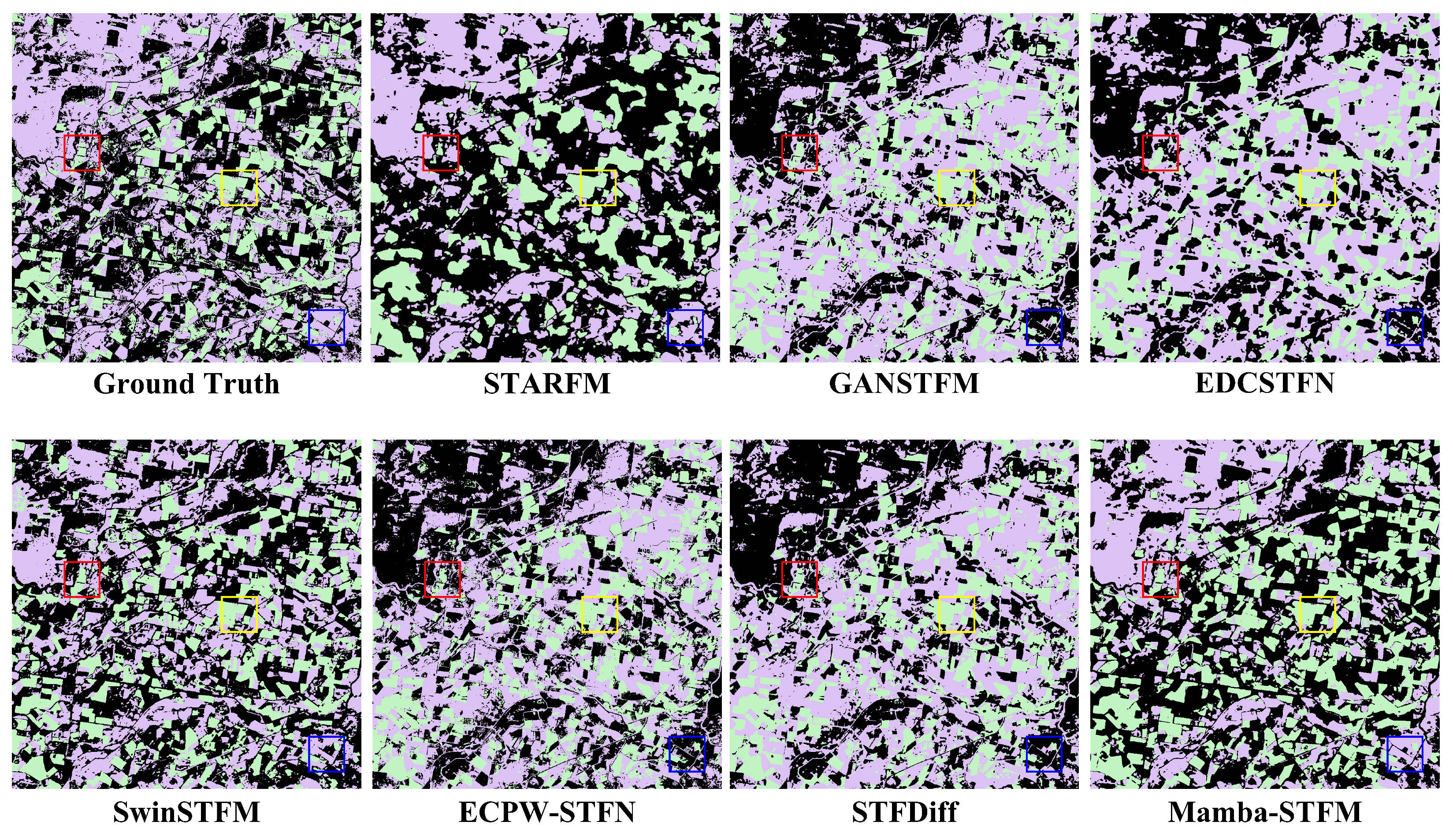
4.5.1. Comparison of Clustering Results in the CIA Study Area

Figure 8 presents the land cover classification results derived from unsupervised K-means clustering applied to the fused images generated by various spatiotemporal fusion models (including STARFM, GANSTFM, EDCSTFN, SwinSTFM, ECPW-STFN, STFDiff, and the proposed Mamba-STFM), as well as the ground truth image, within the CIA study area focused on cropland phenology. By comparing the classification results with the ground truth, we can evaluate each model’s ability to capture surface complexity and phenological variation. As shown in the figure, the classification results of the traditional method STARFM exhibit significant discrepancies from the ground truth in terms of spatial details and class boundaries, manifesting as blurred edges, fragmented features, and misclassifications. Among deep learning methods, GANSTFM and EDCSTFN demonstrate noticeable improvements over STARFM, yet still suffer from classification errors, blurring, and spectral distortions. SwinSTFM, ECPW-STFN, and STFDiff further improve classification performance to a certain extent, capturing more spatial detail. Notably, the classification results based on the fused image generated by the proposed Mamba-STFM method show the highest consistency with the ground truth. Mamba-STFM not only accurately identifies and distinguishes between various land cover types (e.g., cropland, vegetation, bare soil), but also preserves parcel boundaries and internal texture structures with high fidelity. In particular, within the marked regions of interest (highlighted in red, yellow, and blue boxes), the classification results of Mamba-STFM are nearly identical to the ground truth in terms of detail, shape, and spatial layout, significantly outperforming all other methods. These results strongly demonstrate that Mamba-STFM can generate high-quality spatiotemporal fused images, effectively capturing complex cropland phenological dynamics, thereby laying a solid foundation for accurate land cover classification and change detection. The classification results provide intuitive and compelling evidence of the superior performance of Mamba-STFM in spatiotemporal fusion tasks.

Figure 9 illustrates the pixel-level scatter distributions of RED (red dots) and NIR (blue dots) bands between the fused images generated by different spatiotemporal fusion methods and the corresponding ground truth images in the CIA study area. The x-axis represents pixel values from the fused images, and the y-axis shows values from the ground truth. The black dashed line indicates perfect agreement (1:1 correspondence). These scatter plots provide a visual assessment of each method’s ability to reproduce actual surface reflectance at the pixel level, which is especially critical for vegetation index calculations such as NDVI that rely on RED and NIR bands. As shown in the figure, the scatter distributions from STARFM, ESTARFM, GANSTFM, and EDCSTFN are relatively dispersed, with point clouds deviating from the 1:1 line, particularly in high-value regions. This indicates that these methods exhibit substantial errors and uncertainty in predicting surface reflectance and fail to fully capture complex phenological dynamics and surface details. Some deep learning-based methods, such as SwinSTFM, ECPW-STFN, and STFDiff, partially improve the clustering of scatter points, yet still display noticeable outliers and deviations from the 1:1 line. In contrast, the scatter plots generated by the proposed Mamba-STFM model demonstrate superior performance. The scatter points for both RED and NIR bands cluster closely around the 1:1 diagonal line with the lowest degree of dispersion, although some outliers remain. These results strongly indicate that the Mamba-STFM model can predict and reconstruct surface reflectance in the RED and NIR bands with high accuracy, achieving excellent pixel-level consistency with the ground truth. This high-precision spectral reconstruction capability provides a reliable data foundation for remote sensing applications that depend on accurate spectral information, such as precision agriculture monitoring and land cover classification.

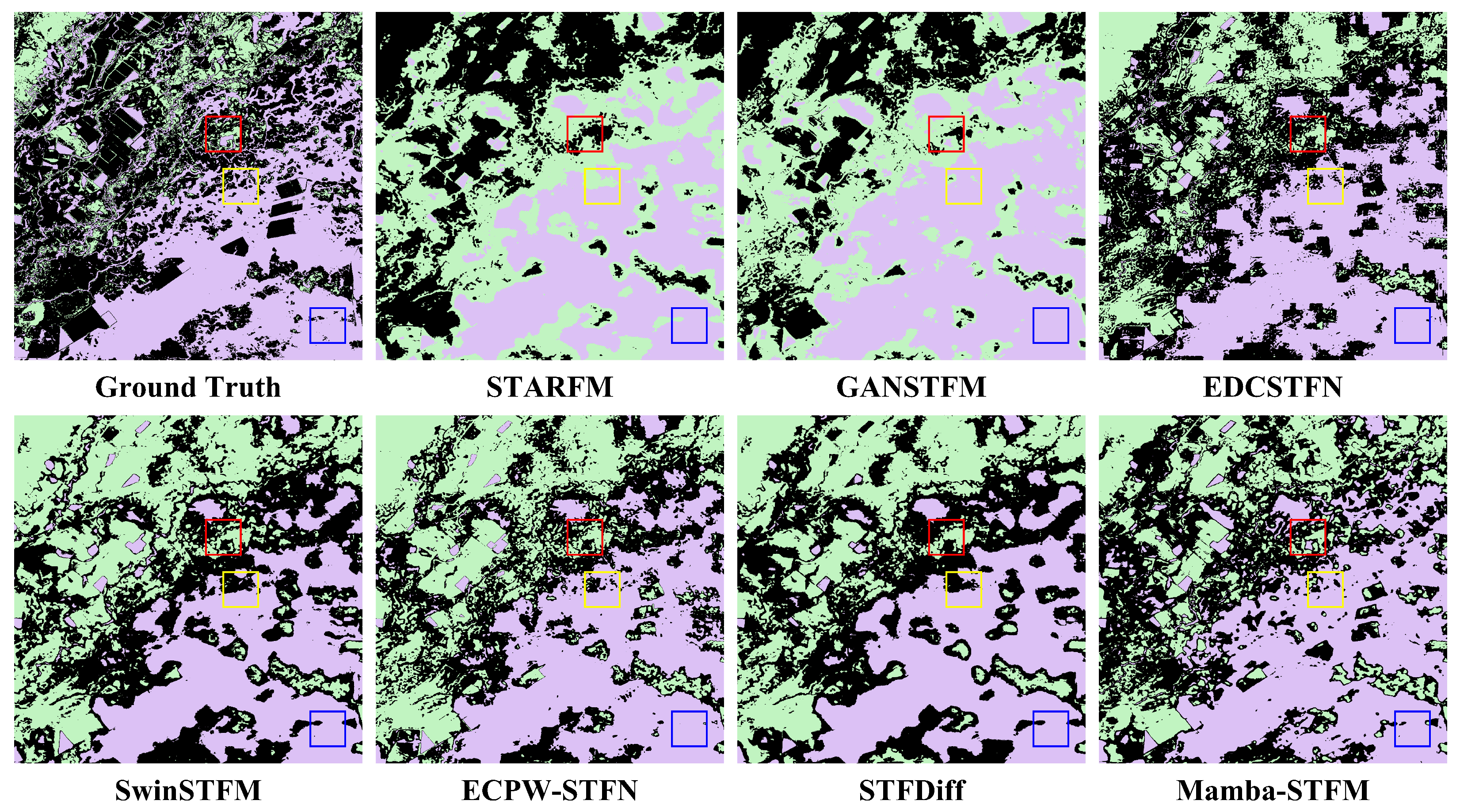
4.5.2. Comparison of Clustering Results in the LGC Study Area

Figure 10 presents the land cover classification results obtained by applying unsupervised K-means clustering to the fused images generated by various spatiotemporal fusion models, alongside the ground truth in the LGC study area, which focuses on flood-induced land cover conflicts. Compared with the ground truth, STARFM exhibits pronounced block effects along complex land cover boundaries, with poor identification of small patches and significant boundary misalignment. Although GANSTFM improves global structure reconstruction to some extent, its classification results are overly smoothed, significantly weakening the micro-scale spatial heterogeneity in flood-affected conflict zones. EDCSTFN demonstrates good alignment with the large-scale distribution of vegetation and bare land but fails to represent small-scale features in conflict zones, leading to frequent local misclassification. SwinSTFM enhances the depiction of patch edge details through window-based self-attention mechanisms, while ECPW-STFN leverages hierarchical convolutions and a progressively weighted multi-scale context aggregation strategy to adaptively assign weights to features of different resolutions. Nevertheless, both methods struggle to fully reconstruct the fragmented spatial patterns induced by subtle floodplain topographies. STFDiff improves texture retention in high-contrast regions, but the overall category distribution still deviates from the actual conditions. In contrast, Mamba-STFM achieves an optimal balance between multi-scale feature fusion and spatiotemporal interaction modeling, accurately reproducing patch shapes and spatial distribution, but also retaining the highest level of micro-scale heterogeneity in flood-induced conflict zones, significantly improving classification accuracy and boundary resolution.

Figure 11 illustrates the scatter distributions of pixel values in the RED (red points) and NIR (blue points) bands between the fused images generated by various spatiotemporal fusion methods and the corresponding ground truth in the LGC study area. The overall trends reveal significant differences in the ability of each method to reproduce pixel-level surface reflectance. Specifically, STARFM and ESTARFM tend to underestimate reflectance in the medium-to-high range, with scattered points widely deviating from the 1:1 reference line. GANSTFM shows some improvement in the high reflectance range but exhibits substantial dispersion in the low reflectance region. EDCSTFN and ECPW-STFN display signs of dynamic range compression; their scatter points are more aligned along the diagonal but generally shift toward the mid-to-low value region. In contrast, SwinSTFM, STFDiff, and Mamba-STFM produce scatter distributions that closely align with the 1:1 reference line, especially at the high reflectance end, where deviations are minimal. This indicates that these three methods exhibit superior performance in reproducing pixel-level surface reflectance. Such accuracy contributes directly to improving the precision of vegetation indices (e.g., NDVI) derived from the RED and NIR bands.

5. Discussion

In this study, we introduce for the first time the Mamba architecture into the spatiotemporal fusion of remote sensing imagery, proposing the Mamba-STFM model. By integrating a linear complexity visual state space (VSS) module and a FuseCore-AttNet attention block within the encoder, alongside a dual “spatial expert” and “temporal expert” mixture-of-experts structure in the decoder, our design efficiently captures both global and local features. This approach overcomes the quadratic computational bottleneck of conventional Transformers while preserving fine-grained spatial details and modeling short-range temporal dependencies, thereby establishing a novel paradigm for spatiotemporal fusion.

Extensive experiments on two public benchmarks (CIA and LGC) demonstrate that Mamba-STFM outperforms seven state-of-the-art methods— including STARFM, GAN-STFM, Swin-STFM, and the recent diffusion-based STFDiff—across all evaluation metrics. For instance, on the CIA dataset, Mamba-STFM achieves the lowest ERGAS (0.8615) alongside the highest SSIM, UIQI, and CC scores; on the LGC dataset, it records an ERGAS of 1.2472, substantially better than the runner-up’s 1.4260. These results confirm the model’s superiority in maintaining spatial fidelity and spectral consistency.

Compared with alternative deep-learning approaches, our VSS-FCAN module leverages parallel scanning and kernel fusion to deliver linear-time global receptive fields, significantly reducing both computational load and memory usage. On an RTX 3090 GPU, Mamba-STFM achieves a 20–30% increase in inference throughput versus traditional GAN- and Transformer-based models while keeping parameter counts and FLOPs at practical levels, underscoring its promise for industrial deployment.

The proposed Mamba-STFM model not only achieves high-quality spatiotemporal fusion but also demonstrates strong potential for real-world applications such as change detection, crop monitoring, and land cover classification. By effectively capturing both spatial and temporal dependencies, it produces semantically meaningful features that support accurate identification of land use changes, vegetation dynamics, and thematic mapping. Preliminary results show that the fused outputs align well with known land cover types, indicating that Mamba-STFM is a scalable and practical tool for downstream Earth observation tasks.

Despite its strong performance, Mamba-STFM generalization under challenging conditions—such as cloud cover, high-latitude polar regions, or abrupt weather changes—remains to be thoroughly evaluated. Furthermore, the efficiency of distributed training across multiple GPUs with very high-resolution inputs warrants further optimization.

6. Conclusions

This study is the first to introduce the Mamba architecture into the domain of remote sensing image spatiotemporal fusion, proposing an end-to-end method named Mamba-STFM. This novel approach expands the design paradigm and application scope of fusion models, providing a new framework for the efficient processing of high-resolution and multitemporal remote sensing data.

The proposed Mamba-STFM consists of three core modules: the VSS-FCAN block, spatial expert, and temporal expert. The VSS-FCAN block significantly reduces quadratic computational complexity and memory overhead while achieving higher inference throughput. The spatial expert adopts an enhanced 2D residual convolution module with channel attention to adaptively recalibrate feature channel weights, thus optimizing spatial feature representation. The temporal expert employs a 3D residual convolution module across adjacent time steps to efficiently capture short-range temporal dependencies with linear sequential modeling complexity.

Comprehensive experiments conducted on the publicly available CIA and LGC datasets demonstrate that Mamba-STFM consistently outperforms existing fusion methods. Quantitatively, it achieves a 1.50%–20.09% improvement in the average correlation coefficient (CC) over all baselines. In terms of qualitative evaluation, Mamba-STFM produces fusion results that are most visually consistent with ground truth. Efficiency-wise, it shows the best balance between computational cost and fusion accuracy. Furthermore, in downstream applications such as land cover classification and change detection, Mamba-STFM exhibits strong practical potential. In summary, Mamba-STFM offers a powerful and scalable solution for remote sensing image fusion tasks and holds significant promise for future development and deployment in real-world Earth observation applications.

Beyond pixel-level fusion, clustering of spatiotemporal features is critical for downstream applications such as land cover classification and change detection. In the context of Mamba-STFM, the rich joint embeddings produced by the VSS-FCAN and the mixture-of-experts decoder naturally lend themselves to unsupervised grouping: the global context captured by the visual state space supports the separation of broad thematic classes, while the fine-grained attention in FuseCore-AttNet preserves local texture cues essential for delineating subtle boundaries. Preliminary experiments have shown that clusters correspond well to known land cover types. This indicates that Mamba-STFM not only excels at image reconstruction but also produces semantically meaningful features suited for clustering-based analyses.

Although Mamba-STFM demonstrates outstanding performance in spatiotemporal fusion tasks, its multi-branch and multi-module architecture inevitably introduces considerable parameter redundancy and high demand for GPU resources during both training and inference. Therefore, our future work will focus on optimizing the network architecture to reduce parameter redundancy and improve fusion efficiency.

References

1. Defourny, P.; Bontemps, S.; Bellemans, N.; Cara, C.; Dedieu, G.; Guzzonato, E.; Hagolle, O.; Inglada, J.; Nicola, L.; Rabaute, T.; et al. Near real-time agriculture monitoring at national scale at parcel resolution: Performance assessment of the Sen2-Agri automated system in various cropping systems around the world. Remote Sens. Environ. 2019, 221, 551–568. [Google Scholar] [CrossRef]
2. Yuan, Q.; Shen, H.; Li, T.; Li, Z.; Li, S.; Jiang, Y.; Xu, H.; Tan, W.; Yang, Q.; Wang, J.; et al. Deep learning in environmental remote sensing: Achievements and challenges. Remote Sens. Environ. 2020, 241, 111716. [Google Scholar] [CrossRef]
3. Du, Z.; Li, X.; Miao, J.; Huang, Y.; Shen, H.; Zhang, L. Concatenated deep-learning framework for multitask change detection of optical and SAR images. IEEE J. Sel. Top. Appl. Earth Obs. Remote Sens. 2023, 17, 719–731. [Google Scholar] [CrossRef]
4. Doña, C.; Chang, N.B.; Caselles, V.; Sánchez, J.M.; Camacho, A.; Delegido, J.; Vannah, B.W. Integrated satellite data fusion and mining for monitoring lake water quality status of the Albufera de Valencia in Spain. J. Environ. Manag. 2015, 151, 416–426. [Google Scholar] [CrossRef]
5. Zhong, L.; Dzurisin, D.; Jung, H.; Zhang, J.; Zhang, Y. Radar image and data fusion for natural hazards characterisation. Int. J. Image Data Fusion 2010, 1, 217–242. [Google Scholar]
6. Shao, Z.; Wu, W.; Li, D. Spatio-temporal-spectral observation model for urban remote sensing. Geo-Spat. Inf. Sci. 2021, 24, 372–386. [Google Scholar] [CrossRef]
7. Xiao, J.; Aggarwal, A.K.; Duc, N.H.; Arya, A.; Rage, U.K.; Avtar, R. A review of remote sensing image spatiotemporal fusion: Challenges, applications and recent trends. Remote Sens. Appl. Soc. Environ. 2023, 32, 101005. [Google Scholar] [CrossRef]
8. Li, J.; Li, Y.; He, L.; Chen, J.; Plaza, A. Spatio-temporal fusion for remote sensing data: An overview and new benchmark. Sci. China Inf. Sci. 2020, 63, 140301. [Google Scholar] [CrossRef]
9. Shen, H.; Meng, X.; Zhang, L. An integrated framework for the spatio–temporal–spectral fusion of remote sensing images. IEEE Trans. Geosci. Remote Sens. 2016, 54, 7135–7148. [Google Scholar] [CrossRef]
10. Roy, D.P.; Wulder, M.A.; Loveland, T.R.; Woodcock, C.E.; Allen, R.G.; Anderson, M.C.; Helder, D.; Irons, J.R.; Johnson, D.M.; Kennedy, R.; et al. Landsat-8: Science and product vision for terrestrial global change research. Remote Sens. Environ. 2014, 145, 154–172. [Google Scholar] [CrossRef]
11. Justice, C.O.; Vermote, E.; Townshend, J.R.; Defries, R.; Roy, D.P.; Hall, D.K.; Salomonson, V.V.; Privette, J.L.; Riggs, G.; Strahler, A.; et al. The Moderate Resolution Imaging Spectroradiometer (MODIS): Land remote sensing for global change research. IEEE Trans. Geosci. Remote Sens. 1998, 36, 1228–1249. [Google Scholar] [CrossRef]
12. Barnes, W.L.; Salomonson, V.V. MODIS: A global imaging spectroradiometer for the Earth Observing System. In Optical Technologies for Aerospace Sensing: A Critical Review; SPIE: St. Bellingham, WA, USA, 1992; Volume 10269, pp. 280–302. [Google Scholar]
13. Zhu, X.; Cai, F.; Tian, J.; Williams, T.K.A. Spatiotemporal fusion of multisource remote sensing data: Literature survey, taxonomy, principles, applications, and future directions. Remote Sens. 2018, 10, 527. [Google Scholar] [CrossRef]
14. Belgiu, M.; Stein, A. Spatiotemporal image fusion in remote sensing. Remote Sens. 2019, 11, 818. [Google Scholar] [CrossRef]
15. Gao, F.; Masek, J.; Schwaller, M.; Hall, F. On the blending of the Landsat and MODIS surface reflectance: Predicting daily Landsat surface reflectance. IEEE Trans. Geosci. Remote Sens. 2006, 44, 2207–2218. [Google Scholar]
16. Zhu, X.; Chen, J.; Gao, F.; Chen, X.; Masek, J.G. An enhanced spatial and temporal adaptive reflectance fusion model for complex heterogeneous regions. Remote Sens. Environ. 2010, 114, 2610–2623. [Google Scholar] [CrossRef]
17. Zhukov, B.; Oertel, D.; Lanzl, F.; Reinhackel, G. Unmixing-based multisensor multiresolution image fusion. IEEE Trans. Geosci. Remote Sens. 1999, 37, 1212–1226. [Google Scholar] [CrossRef]
18. Lu, M.; Chen, J.; Tang, H.; Rao, Y.; Yang, P.; Wu, W. Land cover change detection by integrating object-based data blending model of Landsat and MODIS. Remote Sens. Environ. 2016, 184, 374–386. [Google Scholar] [CrossRef]
19. Wang, Q.; Atkinson, P.M. Spatio-temporal fusion for daily Sentinel-2 images. Remote Sens. Environ. 2018, 204, 31–42. [Google Scholar] [CrossRef]
20. Tan, Z.; Di, L.; Zhang, M.; Guo, L.; Gao, M. An enhanced deep convolutional model for spatiotemporal image fusion. Remote Sens. 2019, 11, 2898. [Google Scholar] [CrossRef]
21. Liao, C.; Wang, J.; Pritchard, I.; Liu, J.; Shang, J. A spatio-temporal data fusion model for generating NDVI time series in heterogeneous regions. Remote Sens. 2017, 9, 1125. [Google Scholar] [CrossRef]
22. Ghosh, R.; Gupta, P.K.; Tolpekin, V.; Srivastav, S. An enhanced spatiotemporal fusion method–Implications for coal fire monitoring using satellite imagery. Int. J. Appl. Earth Obs. Geoinf. 2020, 88, 102056. [Google Scholar] [CrossRef]
23. Dong, R.; Zhang, L.; Fu, H. RRSGAN: Reference-based super-resolution for remote sensing image. IEEE Trans. Geosci. Remote Sens. 2021, 60, 5601117. [Google Scholar] [CrossRef]
24. Wu, M.; Niu, Z.; Wang, C.; Wu, C.; Wang, L. Use of MODIS and Landsat time series data to generate high-resolution temporal synthetic Landsat data using a spatial and temporal reflectance fusion model. J. Appl. Remote Sens. 2012, 6, 063507. [Google Scholar]
25. Lu, L.; Huang, Y.; Di, L.; Hang, D. A new spatial attraction model for improving subpixel land cover classification. Remote Sens. 2017, 9, 360. [Google Scholar] [CrossRef]
26. Zhu, X.; Helmer, E.H.; Gao, F.; Liu, D.; Chen, J.; Lefsky, M.A. A flexible spatiotemporal method for fusing satellite images with different resolutions. Remote Sens. Environ. 2016, 172, 165–177. [Google Scholar] [CrossRef]
27. Wang, S.; Wang, C.; Zhang, C.; Xue, J.; Wang, P.; Wang, X.; Wang, W.; Zhang, X.; Li, W.; Huang, G.; et al. A classification-based spatiotemporal adaptive fusion model for the evaluation of remotely sensed evapotranspiration in heterogeneous irrigated agricultural area. Remote Sens. Environ. 2022, 273, 112962. [Google Scholar] [CrossRef]
28. Guo, D.; Shi, W.; Hao, M.; Zhu, X. FSDAF 2.0: Improving the performance of retrieving land cover changes and preserving spatial details. Remote Sens. Environ. 2020, 248, 111973. [Google Scholar] [CrossRef]
29. Xue, J.; Leung, Y.; Fung, T. A Bayesian data fusion approach to spatio-temporal fusion of remotely sensed images. Remote Sens. 2017, 9, 1310. [Google Scholar] [CrossRef]
30. Li, A.; Bo, Y.; Zhu, Y.; Guo, P.; Bi, J.; He, Y. Blending multi-resolution satellite sea surface temperature (SST) products using Bayesian maximum entropy method. Remote Sens. Environ. 2013, 135, 52–63. [Google Scholar] [CrossRef]
31. Huang, B.; Song, H. Spatiotemporal reflectance fusion via sparse representation. IEEE Trans. Geosci. Remote Sens. 2012, 50, 3707–3716. [Google Scholar] [CrossRef]
32. Song, H.; Huang, B. Spatiotemporal satellite image fusion through one-pair image learning. IEEE Trans. Geosci. Remote Sens. 2012, 51, 1883–1896. [Google Scholar] [CrossRef]
33. Song, H.; Liu, Q.; Wang, G.; Hang, R.; Huang, B. Spatiotemporal satellite image fusion using deep convolutional neural networks. IEEE J. Sel. Top. Appl. Earth Obs. Remote Sens. 2018, 11, 821–829. [Google Scholar] [CrossRef]
34. Tan, Z.; Yue, P.; Di, L.; Tang, J. Deriving high spatiotemporal remote sensing images using deep convolutional network. Remote Sens. 2018, 10, 1066. [Google Scholar] [CrossRef]
35. Liu, X.; Deng, C.; Chanussot, J.; Hong, D.; Zhao, B. StfNet: A two-stream convolutional neural network for spatiotemporal image fusion. IEEE Trans. Geosci. Remote Sens. 2019, 57, 6552–6564. [Google Scholar] [CrossRef]
36. Cheng, F.; Fu, Z.; Tang, B.; Huang, L.; Huang, K.; Ji, X. Stf-egfa: A remote sensing spatiotemporal fusion network with edge-guided feature attention. Remote Sens. 2022, 14, 3057. [Google Scholar] [CrossRef]
37. Li, Y.; Li, J.; He, L.; Chen, J.; Plaza, A. A new sensor bias-driven spatio-temporal fusion model based on convolutional neural networks. Sci. China Inf. Sci. 2020, 63, 140302. [Google Scholar] [CrossRef]
38. Zhang, H.; Song, Y.; Han, C.; Zhang, L. Remote sensing image spatiotemporal fusion using a generative adversarial network. IEEE Trans. Geosci. Remote Sens. 2020, 59, 4273–4286. [Google Scholar] [CrossRef]
39. Song, B.; Liu, P.; Li, J.; Wang, L.; Zhang, L.; He, G.; Chen, L.; Liu, J. MLFF-GAN: A multilevel feature fusion with GAN for spatiotemporal remote sensing images. IEEE Trans. Geosci. Remote Sens. 2022, 60, 4410816. [Google Scholar] [CrossRef]
40. Liu, H.; Yang, G.; Deng, F.; Qian, Y.; Fan, Y. MCBAM-GAN: The GAN spatiotemporal fusion model based on multiscale and CBAM for remote sensing images. Remote Sens. 2023, 15, 1583. [Google Scholar] [CrossRef]
41. Chen, J.; Wang, L.; Feng, R.; Liu, P.; Han, W.; Chen, X. CycleGAN-STF: Spatiotemporal fusion via CycleGAN-based image generation. IEEE Trans. Geosci. Remote Sens. 2020, 59, 5851–5865. [Google Scholar] [CrossRef]
42. Tan, Z.; Gao, M.; Li, X.; Jiang, L. A flexible reference-insensitive spatiotemporal fusion model for remote sensing images using conditional generative adversarial network. IEEE Trans. Geosci. Remote Sens. 2021, 60, 5601413. [Google Scholar] [CrossRef]
43. Vaswani, A.; Shazeer, N.; Parmar, N.; Uszkoreit, J.; Jones, L.; Gomez, A.N.; Kaiser, Ł.; Polosukhin, I. Attention is all you need. In Proceedings of the Advances in Neural Information Processing Systems 30 (NIPS 2017), Long Beach, CA, USA, 4–9 December 2017; pp. 6000–6010. [Google Scholar]
44. Li, W.; Cao, D.; Peng, Y.; Yang, C. MSNet: A multi-stream fusion network for remote sensing spatiotemporal fusion based on transformer and convolution. Remote Sens. 2021, 13, 3724. [Google Scholar] [CrossRef]
45. Chen, G.; Jiao, P.; Hu, Q.; Xiao, L.; Ye, Z. SwinSTFM: Remote sensing spatiotemporal fusion using Swin transformer. IEEE Trans. Geosci. Remote Sens. 2022, 60, 5410618. [Google Scholar] [CrossRef]
46. Jiang, M.; Shao, H. A cnn-transformer combined remote sensing imagery spatiotemporal fusion model. IEEE J. Sel. Top. Appl. Earth Obs. Remote Sens. 2024, 17, 13995–14009. [Google Scholar] [CrossRef]
47. Hu, M.; Wu, C.; Du, B. EMS-Net: Efficient multi-temporal self-attention for hyperspectral change detection. In Proceedings of the IGARSS 2023–2023 IEEE International Geoscience and Remote Sensing Symposium, Pasadena, CA, USA, 16–21 July 2023; pp. 6664–6667. [Google Scholar]
48. Metz, L.; Poole, B.; Pfau, D.; Sohl-Dickstein, J. Unrolled generative adversarial networks. arXiv 2016, arXiv:1611.02163. [Google Scholar]
49. Gulrajani, I.; Ahmed, F.; Arjovsky, M.; Dumoulin, V.; Courville, A.C. Improved training of wasserstein gans. In Proceedings of the Advances in Neural Information Processing Systems 30 (NIPS 2017), Long Beach, CA, USA, 4–9 December 2017; pp. 5769–5779. [Google Scholar]
50. Liu, Y.; Tian, Y.; Zhao, Y.; Yu, H.; Xie, L.; Wang, Y.; Ye, Q.; Jiao, J.; Liu, Y. Vmamba: Visual state space model. In Proceedings of the Advances in Neural Information Processing Systems 37 (NIPS 2024), Vancouver, BC, Canada, 10–15 December 2024; pp. 103031–103063. [Google Scholar]
51. Emelyanova, I.; McVicar, T.; Van Niel, T.; Li, L.; Van Dijk, A. Landsat and MODIS data for the Coleambally Irrigation Area; v3. Data Collection; CSIRO: Canberra, Australia, 2013. [Google Scholar] [CrossRef]
52. Emelyanova, I.; McVicar, T.; Van Niel, T.; Li, L.; Van Dijk, A. Landsat and MODIS Data for the Lower Gwydir Catchment Study Site; v3. Data Collection; CSIRO: Canberra, Australia, 2013. [Google Scholar] [CrossRef]
53. Zhang, X.; Li, S.; Tan, Z.; Li, X. Enhanced wavelet based spatiotemporal fusion networks using cross-paired remote sensing images. ISPRS J. Photogramm. Remote Sens. 2024, 211, 281–297. [Google Scholar] [CrossRef]
54. Huang, H.; He, W.; Zhang, H.; Xia, Y.; Zhang, L. STFDiff: Remote sensing image spatiotemporal fusion with diffusion models. Inf. Fusion 2024, 111, 102505. [Google Scholar] [CrossRef]
Figure 1. The overall architecture of the Mamba-STFM model and the structure of the VSS-FCAN block.
Remotesensing 17 02135 g001
Figure 2. Network architecture diagram of FuseCore-AttNet.
Remotesensing 17 02135 g002
Figure 3. Network structure diagram of the STF-MoE block.
Remotesensing 17 02135 g003
Figure 4. Detailed comparison of different fusion products with ground truth values on the CIA dataset.
Remotesensing 17 02135 g004
Figure 5. RMSE error map of different fusion products on the CIA dataset.
Remotesensing 17 02135 g005
Figure 6. Detailed comparison of different fusion products with ground truth values on the LGC dataset.
Remotesensing 17 02135 g006
Figure 7. RMSE error map of different fusion products on the LGC dataset.
Remotesensing 17 02135 g007
Figure 8. K-means clustering results of fused images by various methods in the CIA region, where green represents Class 1 and purple represents Class 2.
Remotesensing 17 02135 g008
Figure 9. Scatter distribution of pixel values between different fused images and the corresponding real images in the RED and NIR bands within the CIA study area.
Remotesensing 17 02135 g009
Figure 10. K-means clustering results of fused images by various methods in the LGC region, where green represents Class 1 and purple represents Class 2.
Remotesensing 17 02135 g010
Figure 11. Scatter distribution of pixel values between different fused images and the corresponding real images in the RED and NIR bands within the LGC study area.
Remotesensing 17 02135 g011