Image Characteristic-Guided Learning Method for Remote-Sensing Image Inpainting

Abstract

Inpainting noisy remote-sensing images can reduce the cost of acquiring remote-sensing images (RSIs). Since RSIs contain complex land structure features and concentrated obscured areas, existing inpainting methods often produce color inconsistency and structural smoothing when applied to RSIs with a high missing ratio. To address these problems, inspired by tensor recovery, a lightweight image Inpainting Generative Adversarial Network (GAN) method combining low-rankness and local-smoothness (IGLL) is proposed. IGLL utilizes the low-rankness and local-smoothness characteristics of RSIs to guide the deep-learning inpainting. Based on the strong low rankness characteristic of the RSIs, IGLL fully utilizes the background information for foreground inpainting and constrains the consistency of the key ranks. Based on the low smoothness characteristic of the RSIs, learnable edges and structure priors are designed to enhance the non-smoothness of the results. Specifically, the generator of IGLL consists of a pixel-level reconstruction net (PIRN) and a perception-level reconstruction net (PERN). In PIRN, the proposed global attention module (GAM) establishes long-range pixel dependencies. GAM performs precise normalization and avoids overfitting. In PERN, the proposed flexible feature similarity module (FFSM) computes the similarity between background and foreground features and selects a reasonable feature for recovery. Compared with existing works, FFSM improves the fineness of feature matching. To avoid the problem of local-smoothness in the results, both the generator and discriminator utilize the structure priors and learnable edges to regularize large concentrated missing regions. Additionally, IGLL incorporates mathematical constraints into deep-learning models. A singular value decomposition (SVD) loss item is proposed to model the low-rankness characteristic, and it constrains feature consistency. Extensive experiments demonstrate that the proposed IGLL performs favorably against state-of-the-art methods in terms of the reconstruction quality and computation costs, especially on RSIs with high mask ratios. Moreover, our ablation studies reveal the effectiveness of GAM, FFSM, and SVD loss. Source code is publicly available on GitHub.

1. Introduction

The absence of large concentrated region pixels is frequently observed in visible remote-sensing images (RSIs). This is primarily because approximately 60% of the Earth’s surface is covered by clouds [1], which results in unavailable pixels [2]. Additionally, when large-area focal array planes are mosaicked to acquire texture details and spatial information, mosaicking gaps or pixel loss often occur [3]. Meanwhile, imaging conditions (e.g., uneven illumination or atmospheric interference) and hardware malfunctions also induce the loss of strip information [4].

Image inpainting is a long-standing challenging task in computer vision, aiming to recover the missing regions with plausible pixels. Since the cost of acquiring remote-sensing images is high, inpainting RSIs with missing areas can gain substantial practical significance for cost-efficiency. Inpainting RSIs that contain complex ground object information has sparked intense discussions in many research works [5,6]. The repaired RSIs can be used for tasks such as detection and classification [5]. It is crucial to generate reasonable results for large concentrated missing areas with low computational complexity in practical applications.

Two critical characteristics of tensor data—low-rankness and smoothness—have achieved success in tensor data recovery [7]. However, they are rarely considered in visible-light image inpainting. Low-rankness refers to the presence of information redundancy in data [8], while smoothness refers to the local continuity of adjacent pixel values [8]. Works [9,10] demonstrate that both low-rankness and smoothness characteristics are also inherent in visible light images. Remote-sensing images (RSIs) exhibit stronger low-rankness due to the abundance of repetitive elements in the imagery. Meanwhile, in scenes such as urban buildings and ports, RSIs show weaker smoothness, primarily because individual pixels often contain complex objects with drastic color variations at object boundaries.

Due to the extensive spatial and temporal coverage in RSIs, low-rankness characteristic exists in the spatial and temporal dimensions. For example, spatial-based methods [11] usually search for a well-matched patch from the remaining information, but it is only suitable for restoring small scale mask [4]. Temporal-based methods [12], consider the autocorrelation of time-series data, employing multi-year or multi-month Landsat images to recover RSIs. Spatiotemporal-based methods [13] leverage the repetitive rank of both the spatial and temporal dimensions. However, these methods require intricate processing with massive human and material resources, increasing the complexity of data collection and lacking the flexibility of the method [14].

In addition to low-rankness, smoothness is also an important prior in the image inpainting field. Smoothness arises in the lightweight learning method field, attributed to a variety of factors. CNN-based methods [14,15,16] tend to produce overly smooth results due to their local inductive priors [9], resulting in structural incoherence. For instance, lightweight CNN-based methods can achieve good results when processing images with less rich feature information such as forests and oceans. When dealing with scenes like parks and cities, issues such as structural distortion and color shift are likely to occur [5]. They cannot function effectively in the inpainting of RSIs with low smoothness. CNN-based models require large receptive fields to preserve holistic structures [17]. To address the limitations of CNN, transformer-based methods [18,19,20] enlarge the receptive fields by establishing long-term correlations. The Pure transformer method [18] often loses fine-grained image details. To tackle this issue, transformer-CNN hybrid methods [19,21,22] impose dual constraints on semantic coherence and detail preservation, enabling the inpainting of texture-rich details. Meanwhile, diffusion-based methods [23,24] learn high-frequency texture details through a sequential framework of forward diffusion process and reverse denoising process, gradually refining noise into realistic image structures. Nevertheless, both transformer-based and diffusion-based methodologies incur significant computational overhead, demanding substantial resources for training and inference.

For lightweight methods, achieving high-quality restoration of RSIs with a large area of concentrated missing regions remains a challenge [25]. Mainstream deep-learning methods, such as the method in [24], tend to achieve inpainting by enhancing the semantic understanding ability of the model, rather than starting from the characteristics of the data. Improving semantic understanding ability will incur greater computational costs, making it not suitable for specific scenarios with insufficient computational resources. Inspired by the work of tensor recovery [8], we have introduced the low-rankness and smoothness characteristics of visible-light remote-sensing data into the deep-learning model. Different from the existing lightweight methods, our method combines image characteristics and the deep-learning method. It improves the model’s understanding of the intrinsic characteristics of the image. Our method can break free from the limitation of insufficient computing power and achieve high-quality inpainting with a low computational cost.

In this paper, we propose a lightweight image inpainting generative adversarial network (GAN) method combining low-rankness and local-smoothness (IGLL) that combines mathematical principles with deep learning. Considering the low-rankness, the proposed singular value decomposition (SVD) loss term restricts the similarity between real and generated images in low-dimensional space, and the proposed GAM and FFSM borrow repetitive elements from the background to inpaint the foreground. These components effectively avoid color shift. Considering the local-smoothness, IGLL employs structural priors and learnable edges to prevent the generated results from being too smooth, thereby avoiding structural distortion. Specifically, IGLL consists of a pixel-level reconstruction network (PIRN) and a perceptual-level reconstruction network (PERN). In PIRN, a global attention module (GAM) is designed for modeling long-range dependencies. Given the limited available information, normalization layers are excluded to avoid distorting limited available features. Additionally, to prevent excessive weight allocation to similar pixels from compromising structural information, the multi-head attention mechanism is omitted. In PERN, a flexible feature similarity module (FFSM) is proposed to fill the foreground by selecting similar representations. FFSM conducts cross-attention on the self-attention scores of the foreground and the background, achieving a fine-grained matching. Extensive experiments demonstrate that the proposed IGLL can generate high-quality results even with concentrated missing regions, generalizing well across various scenarios.

The main contributions of this paper can be summarized as follows.

(1) To recover remote-sensing images (RSI) with high spatial variability and concentrated missing pixels, inspired by tensor recovery, the IGLL method is designed based on the low-rankness characteristic and smoothness of RSI. The proposed global attention module (GAM) and flexible feature similarity module (FFSM), alongside the SVD loss, enhance the model’s exploitation of image low-rank properties. A structure preservation mechanism is designed to mitigate structure distortion resulting from overly smoothing restoration.

(2) The proposed GAM captures the dependency between the background and foreground. To accommodate the complexity of remote-sensing ground truth, the GAM enhances the model’s perceptual capabilities and avoids overfitting. The proposed FFSM couples GAM and transposed convolution to refine the granularity of similarity comparison. The foreground is filled by selecting high-similarity background features. We introduce a novel SVD loss that distills the image into low-rank information. This loss constrains the same low-rank feature between the ground truths and the results in both the generator and the discriminator.

(3) Experimental results demonstrate that the proposed method can restore remote-sensing images with large concentrated missing areas, consuming low computation costs. IGLL outperforms state-of-the-art methods in terms of qualitative and quantitative evaluation.

The rest of the sections in this paper are as follows. Section 2 provides an overview of related work. Section 3 presents the proposed methodology in detail. Section 4 describes the experimental setup and analyses the results. The proposed IGLL is compared with other state-of-the-art algorithms. We also conduct ablation studies about the GAM, FFSM, structure preservation mechanism and SVD loss. Section 5 discusses the reasons for the advantages of our model. Finally, Section 6 concludes the paper.

2. Related Work

2.1. CNN-Based Methods

For CNN-based methods, Hui et al. [26] utilize a densely connected dilated convolutional structure and self-guided regression loss to enhance semantic details. This method encounters missing pixels in the center when inpainting high-resolution images. Yi et al. [27] introduce a contextual residual aggregation (CRA) mechanism to generate high-frequency residual information. It aggregates residual information from contextual pixel blocks through weighted aggregation. The CRA method produces clear high-frequency results through low-resolution predictions, effectively handling high-resolution images. Due to the image scaling operation, the restored images may lack clarity. To adaptively select the features, Wang et al. [28] propose a dynamic selection network (DSNet), utilizing effective pixels through a dynamic selection mechanism. It dynamically selects spatial sampling positions during the convolutional stage to make the feature extraction process flexible. DSNet also incorporates various normalization methods and unstable features to generate more realistic and finer images. Deng et al. [29] propose a HAN to fully use hierarchical features to mine effective information for broken images. However, CNNs are limited in receptive fields. It is hard to learn consistent semantic textures. To ensure structural consistency and fine details, Wang et al. [30] introduce a specialized multi-level attention module to refine textures by swapping small patches. Du et al. [3] propose a coarse-to-fine deep generative model with a spatial semantic attention mechanism. This model ensures the continuity of local features and the relevance of global semantic information. Due to the lack of holistic structure and a comprehensive understanding of large images, CNN-based methods can only deal with the images with small missing areas. When the missing area is excessively large, significant repair artifacts still occur. The above-mentioned CNN-based methods produce over-smooth results when repairing remote-sensing images with large missing regions. It is challenging to recover critical edges and lines within scenes [15].

2.2. Transformer-Based and Diffusion-Based Methods

The transformer-based methods obtain large receptive fields by establishing long-range dependency to generate satisfactory results. He et al. [18] utilize the semantic understanding ability of the transformer to recover images with a high masking ratio. However, the results are often blurry due to the transformer’s limited capacity to capture high-frequency image details. To further enhance inpainting capability, Li et al. [22] combine both transformer and convolution to handle high-resolution images effectively. To preserve the overall structure, Dong et al. [17] propose an incremental transformer enhanced inpainting, achieving significant improvements. Transformer-based methods typically employ downsampling techniques to reduce spatial dimensions, which can result in information loss. To mitigate this issue, Chen et al. introduce HINT [20]. Transformer-based methods leverage powerful semantic understanding capability to prevent generating smooth results.

Diffusion models are generative models that aim to learn a data distribution from samples [31,32]. Recent works [24,33] leverage the detail-generation capability of the stable diffusion (SD) model [34] to complete image-generation tasks rather than image-inpainting tasks.

Transformer-based and diffusion-based methods demand substantial computational overheads, which limits their performance in practical applications when dealing with RSIs.

3. Methodology

In this section, the image characteristics and the overall structure are introduced. Subsequently, the mechanisms designed for low-rankness and smoothness are discussed. Additionally, to further enhance the model’s potential, the GAM, FFSM, and SVD loss functions are designed to leverage these low-rank and smoothness principles.

3.1. The Preliminaries of Low-Rankness and Local-Smoothness

In tensor reconstruction, the intrinsic features (e.g., low-rankness and local-smoothness) of tensor data are leveraged to guide reasonable estimation of missing tensors. Similarly, RSIs exhibit low-rankness and local-smoothness, characteristics to be described in detail later. Low-rankness refers to the redundancy of image information, revealing the information correlation within image data. This characteristic leads to the following low-rankness recovery model:

$${min}_{\mathcal{T}}\Re \left(\mathcal{T}\right)\mathrm{s}.\mathrm{t}.\mathcal{Y}=\mathrm{\Phi }\left(\mathcal{T}\right),$$

(1)

where $\mathcal{Y}=\mathrm{\Phi }\left(\mathcal{T}\right)$ is the observed incomplete image, $\mathcal{T}\in {\mathbb{R}}^{n_1\times n_2\times \cdots \times n_d}$ is the expected complete image information, $\Re \left(\mathcal{T}\right)$ denotes the regularizer measuring tensor low-rankness, and ${min}_{\mathcal{T}}$ denotes finding the tensor $\mathcal{T}$ that minimizes the objective function $\Re \left(\mathcal{T}\right)$ with $\mathcal{T}$ as the optimization variable. Local-smoothness is defined as the property that pixels with low spatial variation exhibit small numerical differences. Adjacent pixels along a tensor mode (e.g., spatial dimension) tend to change continuously, representing information similarity at a local scale. The process of recovering global information from an incomplete image can be modeled as follows:

$${min}_{\mathcal{T}}\Re \left(\mathcal{T}\right)+\alpha \mathfrak{S}\left(\mathcal{T}\right)\mathrm{s}.\mathrm{t}.\mathcal{Y}=\mathrm{\Phi }\left(\mathcal{T}\right),$$

(2)

where $\mathrm{\Phi }\left(\right)$ is the operator modeling certain degradation kernel, $\mathfrak{S}\left(\right)$ represents the regularize for measuring the smoothness characteristic, and $\alpha >0$ is the balance parameter.

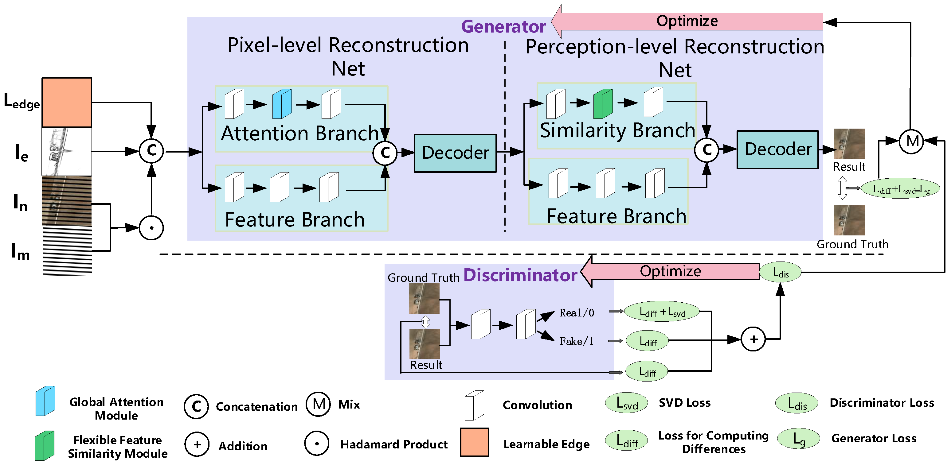
3.2. Network Architecture

The overall architecture of IGLL is based on a conditional GAN. As shown in Figure 1, $I_n$ is the image with hole, $I_e$ is the edge data, and $I_m$ is mask information. To adapt to the complex characteristics of RSIs, we employ CNNs, which are proficient at capturing high-frequency information, as the backbone for RSI inpainting tasks [5]. RSIs have informational complexity, with each pixel containing more substantial data. Therefore, in RSI inpainting tasks, capturing high-frequency detail is paramount. The high-frequency modeling ability of CNNs is superior to that of transformers. Furthermore, CNNs require less computational resources than transformers and diffusion models. Thus, CNNs are chosen as the backbone.

The encoders of PIRN and PERN exhibit structural similarities. A network with extra attention branches and regular branches is designed in the encoder. The attention branch connects different attention modules after an array of convolutional layers and downsampling layers. The feature branch employs dilated convolution to extend the receptive field. The dilated convolutional layers can capture a more extensive context of information, yielding superior performance. In the feature branch, dilation rates are empirically set to 2, 4, 8, and 16, respectively. In the decoder, convolution is used to refine the geometry of objects and recover detailed information. Employing upsampling keeps the image size unchanged and fills the missing regions.

3.3. Mechanisms Designed for Low-Rankness and Local-Smoothness

The low-rankness characteristic makes it easy to find repeated pixels to fill the hole. Due to the low smoothness of RSIs, lightweight methods tend to blur the structure, which are not suitable for RSIs with diversity. To address these issues, IGLL employs a GAM, a FFSM, and an SVD loss to strengthen the low-rankness in the results. Additionally, IGLL exploits a structural preservation mechanism to constrain excessive smoothness in results. The improved design process of IGLL for low-rankness and smoothness is as follows:

$${min}_{\mathcal{T}}\Re \left(\mathcal{T}\right)\uparrow +\alpha \mathfrak{S}\left(\mathcal{T}\right)\downarrow \mathrm{s}.\mathrm{t}.\mathcal{Y}=\mathrm{\Phi }\left(\mathcal{T}\right),$$

(3)

where ↑ indicates that the IGLL model should be designed to enhance its exploitation of the low-rankness characteristics of RSIs to avoid color inconsistency, and ↓ implies that the IGLL model needs to suppress the smoothness characteristics of the results to mitigate the issue of structural over-smoothing. As for low-rankness, the IGLL model needs to fully utilize the low-rankness characteristic of remote-sensing images. To generate pixels that are close to the missing features, the GAM and FFSM attempt to replicate reliable feature information from known background patches, instead of randomly generating foreground information. The GAM module enhances the model’s learning ability and enables pixel-level inpainting. The FFSM module establishes semantic correlations by leveraging the GAM module, providing fine details and enabling semantic-level inpainting.

As for smoothness, the IGLL model needs to suppress the smoothness of the generated results. In the structural preservation mechanism, the structure priors guide images with severe structural damage to maintain structural invariance, and learnable edges assist in modeling structures. The lost data in remote-sensing images are usually relatively concentrated, causing significant disruption to the overall structure. Unlike simple image data such as face images, RSIs have complex features that lightweight models struggle to capture. The edge information and learnable edges play an important role in large-area inpainting tasks. The edge information is obtained by the pixel difference networks (PID) [35]. When edge information is integrated into the model, the optimization objective function transforms from (4) to (5).

$$\begin{array}{cc}\hfill & \underset{G}{min}\underset{D}{max}V(D,G)={\mathbb{E}}_{x\sim p_{\mathrm{data}}\left(x\right)}[logD\left(x\right)]\hfill \\ \hfill & +{\mathbb{E}}_{z\sim p_z\left(z\right)}[log(1-D\left(G\left(z\right)\right))]\hfill \end{array}$$

(4)

$$\begin{array}{cc}\hfill & {min}_G{max}_{D}V(D,G)={\mathbb{E}}_{x\sim p_{\mathrm{data}}\left(x\right)}[logD(x\mid y)]\hfill \\ \hfill & +{\mathbb{E}}_{z\sim p_z\left(z\right)}[log(1-D\left(G(z\mid y)\right))]\hfill \end{array},$$

(5)

where G is the generator, D is the discriminator; $p_{data}$ is the distribution of real data, $p\left(z\right)$ is the distribution of the generator’s input noise, x is a sample from $p_{data}\left(x\right)$, z is a sample from $p\left(z\right)$, and y represents additional edge information.

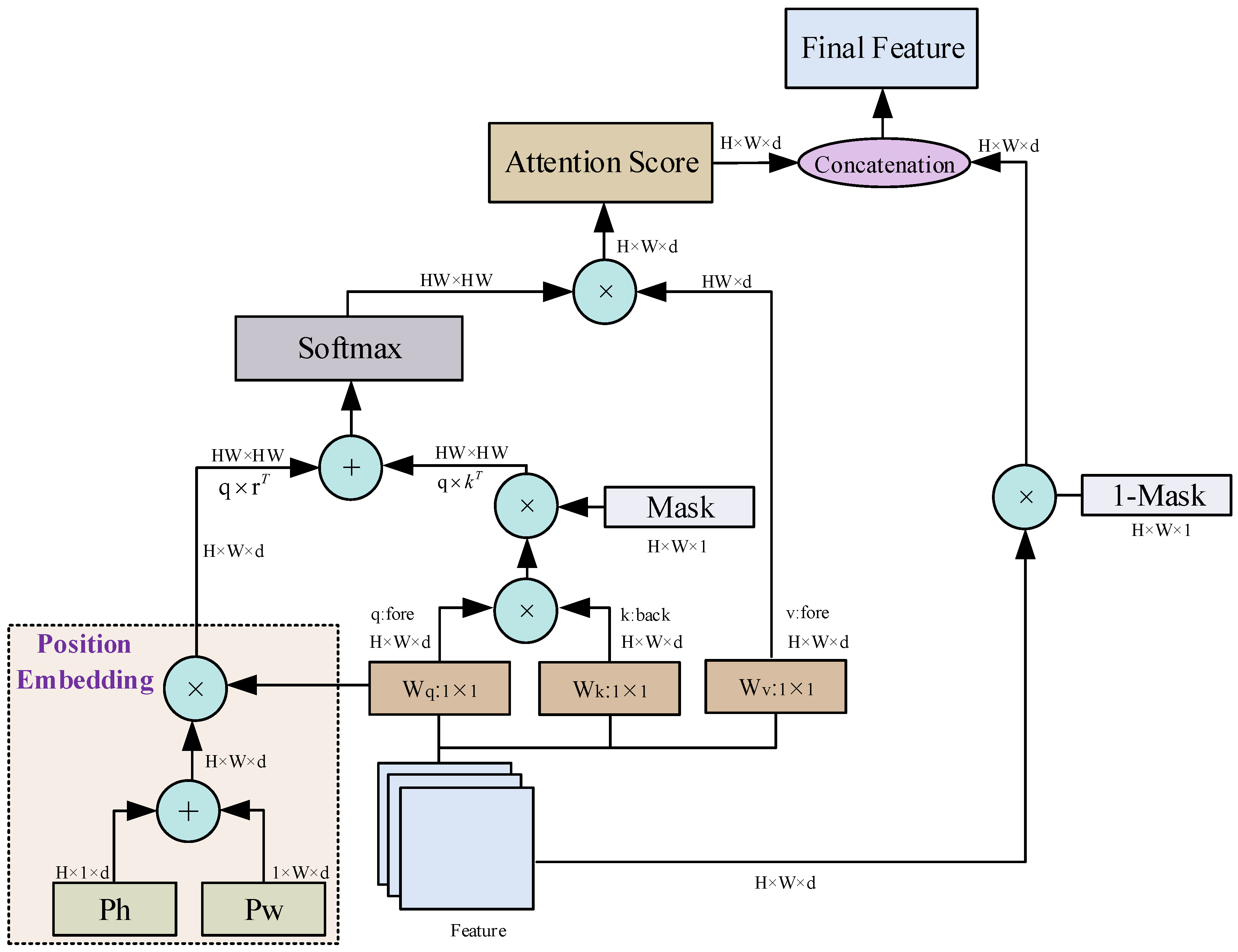
3.4. Global Attention Module

To adapt the attention module in the vanilla transformer [19] to the backbone, we redesign it as the global attention module (GAM). The details of the GAM are shown in Figure 2. Positional encodings for height (Ph) and width (Pw) are introduced to capture the spatial ordering of input tokens. In RSIs, missing areas are often concentrated, making positional information crucial for accurately reconstructing spatial structures during inpainting. Due to the propensity for remote-sensing images to exhibit correlations over long distances, we employ absolute position encodings, akin to the approach used in [36]. The absolute positional encoding vectors are learned through training. For input elements $x_i\in R^{d_x}$, the learnable encoding approach is designed to obtain the absolute positions ($p_i\in R^{d_x}$). Associate ($p_i$) with the query terms, and add ($p_{i}Q$) to the input token embedding x as:

$$x_i=x_i+p_{i}Q,$$

(6)

where Q is query item. The attention mechanism can be defined as follows:

$$Attention(Q,K,V)=\underset{P}{\underbrace{softmax\left({\displaystyle \frac{Q{K}^T}{\sqrt{d}}}\right)}}V.$$

(7)

The content of the multi-head attention mechanism is obtained by:

$$MHSA(Q,K,V)=Concat\left({head}_1,\dots ,{head}_{\mathrm{h}}\right){\mathrm{W}}^{\mathrm{O}},$$

(8)

where ${\mathrm{head}}_{\mathrm{i}}=Attention\left(Q{\mathbb{W}}_{\mathrm{i}}^{\mathbb{Q}},K{\mathbb{W}}_{\mathrm{i}}^{\mathbb{K}},V{\mathbb{W}}_{\mathrm{i}}^{\mathbb{V}}\right)$, ${\mathbb{W}}_{\mathrm{i}}^{\mathbb{Q}}\in {\mathbb{R}}^{m\times d_q}$, ${\mathbb{W}}_{\mathrm{i}}^{\mathbb{K}}\in {\mathbb{R}}^{m\times d_k}$, ${\mathbb{W}}_{\mathrm{i}}^{\mathbb{V}}\in {\mathbb{R}}^{m\times d_v}$, and ${\mathrm{W}}^O\in {\mathbb{R}}^{h{d}_v\times C}$ are learnable parameters, ${\mathrm{d}}_{\mathrm{k}}$ and ${\mathrm{d}}_{\mathrm{v}}$ are the hidden dimensions of the projection subspaces, h is the number of heads, and m is the embedding dimension. In the transformer attention, a multi-head attention mechanism aims to increase the model’s representational capacity and prevent the model from overly focusing on the current positions. However, the multi-head attention allocates more attention to the foreground pixels that closely resemble the background pixels. This not only makes model prone to overfitting on pixels but also results in biases in the structural information. Furthermore, multi-head attention increases the computational complexity, imposing substantial computational costs. To address these issues, we adopt a single-head attention design rather than multi-head attention.

Additionally, to improve the accuracy of the algorithm further, we introduce a mask for image pruning to perform normalization in the foreground. Since the background region is known and does not require processing, the attention mechanism should be concentrated on the foreground information. Using a mask to prune the image normalizes attention scores to the $[0,1]$ range for the foreground information, thereby establishing a more refined global dependencies. For a given mask $M\in {\mathbb{R}}^{H\times W\times 1}$, for each element $M_{ij}$ in the mask matrix M, $M_{ij}=1$ represents a missing pixel, and $M_{ij}=0$ represents an existing pixel. After obtaining the pruned relevance graph, a softmax operation is performed to obtain the probability. The whole process above can be formulated as follows:

$$F_a=\tau [(\mathrm{mask}\odot (Q\times K))+(pos\times (Q\times K))],$$

(9)

where $\tau$ represents the softmax operation, mask is the mask information for the image, $pos$ is the pixel position matrix, Q, K, and V are the query terms, key terms, and value terms in the attention mechanism, $F_a$ represents the final global attention score, and ⊙ denotes the dot product operation. The final predicted output image can be computed as follows:

$$F_o=[(v\times F_a)\times mask]+[F\times (1-mask)],$$

(10)

where $F_o$ represents the output feature, and F represents the original image feature. The addition of a positional vector enhances the network robustness and processing capabilities.

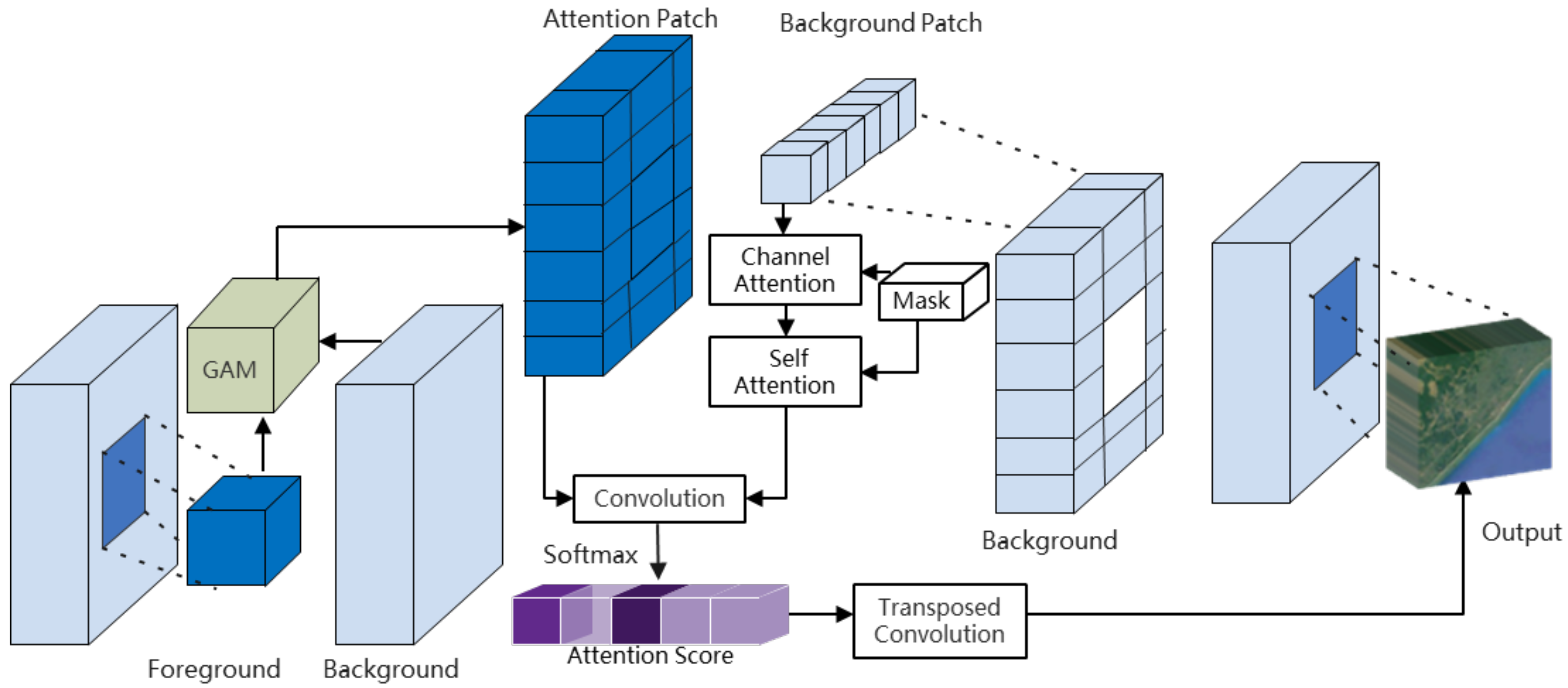
3.5. Flexible Feature Similarity Module

The structure of FFSM in the PERN is shown in Figure 3. The input of PERN is a set of triplets of corresponding images ($x_a$, $x_b$, m), where $x_a$ is the output from the PIRN, $x_b$ is the background information, and m is the mask marking the corrupted regions. The existing work [28] employs dynamic convolution and transposed convolution to achieve flexible feature selection. However, this approach [28] proves ineffective when processing RSIs with significant variations in ground object information, as this method’s feature selection mechanisms are relatively coarse. In RSIs, where even a single pixel may encapsulate critical information, establishing fine-grained associations between background and foreground becomes critical. To perform more refined image restoration, the GAM module establishes semantic-level mappings for both the foreground and background through attention mechanisms, enabling fine-grained feature selection.

Similarity is measured by convolving foreground features with background features to extract cross-region correlations. Based on the similarity scores, relevant background patches are mapped to the foreground region. These mapped background patches are then upsampled via transposed convolution to fill missing regions. The similarity computation can be mathematically formulated as follows:

$$s_{p_b,p_f}^i=〈{\displaystyle \frac{p_b}{∥p_b∥}},{\displaystyle \frac{p_f}{∥p_f∥}}〉,$$

(11)

where $s^i$ represents the similarity between every two image blocks. $p_b$ and $p_f$ represent background information and foreground features, respectively. The similarity score between foreground and background information is calculated by convolving the foreground information as a filter with the background information. Subsequently, a softmax function is applied to normalize the attention scores to the $[0,1]$ range. The softmax function computation is described as:

$${\kappa }_s={\displaystyle \frac{exp\left(s\right)}{\sum _{i}exp\left(s^i\right)}},$$

(12)

where ${\kappa }_s$ represents the desired attention scores, and $s^i$ is the attention of each small block. After the softmax operation, each pixel records attention scores. The block with the highest score is selected as a kernel for transposed convolution to reconstruct the result.

3.6. Loss Function

The loss function consists of perceptual loss ($L_{per}$) [37], style loss ($L_{sty}$) [38], local loss ($L_{local}$) [39], adversarial loss ($L_{adv}$) [40], and the proposed SVD loss. $L_{per}$ is computed from a pre-trained VGG19 [41] network, measuring the gap between generated images and ground truth. $L_{sty}$ measures the Gram matrix of the output image and ground-truth features by using the VGG19 network. $L_{local}$ calculates the foreground differences between output and ground truth. Since the background is already known and unchanged, focusing the loss function on the foreground effectively guides the model to learn critical details. For the generator, $L_{adv}$ encourages it to generate more realistic samples to deceive the discriminator, making the discriminator misjudge them as real. For the discriminator, the $L_{adv}$ enhances its ability to distinguish real samples from fake ones generated by the generator.

SVD [42] loss is usually used to extract the key rank low rank, which means processing images into a low-rank form. The goal is to preserve fine details and complex structures in images. TV is often used to promote smoothness. The goal is to preserve fine details and complex structures in images. Our experiments have shown that adding TV constraints (which promote smoothness) can lead to the loss of important features. Therefore, smoothness regularization is not adopted in this framework. SVD achieves rank control through a multiplicative decomposition framework. SVD establishes a complete algebraic framework for matrix decomposition. The details of SVD are as follows:

$$\begin{array}{c}A=U\Sigma V^T,\hfill \end{array}$$

(13)

where U is an orthogonal matrix whose columns represent the left singular vectors of A. $\Sigma$ is a diagonal matrix containing the singular values, which are non-negative and typically ordered from largest to smallest. $V^T$ is the transpose of an orthogonal matrix whose columns represent the right singular vectors of A. As shown in Figure 1, the SVD calculates the singular values and constrains the key ranks between the foreground and background, enhancing the model’s semantics understanding capability and increasing the visual fidelity. The SVD loss in the generator is defined as:

$$\begin{array}{c}{L}_{\mathrm{svd}}=\mathbb{E}\left[\sum _i^k{∥svd\left(p_i^{gt}\right)-svd\left(p_{\mathrm{i}}^{\mathrm{pred}}\right))∥}_1\right],\hfill \end{array}$$

(14)

where $svd$ is a matrix factorization method that leverages randomized techniques (such as GESVD or Krylov subspace methods [43]) executed on modern graphics processing units (GPUs) to compute matrix decompositions, and $svd\left(p_i^{gt}\right)$ and $svd\left(p_{\mathrm{i}}^{\mathrm{pred}}\right)$ represent the i-th singular values of the ground truth and the predicted result. This approach maps the rank of a matrix to a latent vector space, thereby enabling data dimensionality reduction. The generator aims to generate a result that can deceive the discriminator, making the discriminator unable to distinguish between generated samples and real samples. The training process of the generator is as follows:

$$\begin{array}{c}{L}_G=-{\mathbb{E}}_{z\sim p_z\left(z\right)}[logD\left(G\left(z\right)\right)],\end{array}$$

(15)

where z is a random noise vector drawn from a prior distribution $p_z$. $G\left(z\right)$ is the sample generated by the generator. $D\left(G\right(z\left)\right)$ represents the discriminator’s probability score for the generated sample being real. The goal of training the generator is to minimize the loss $L_G$. The loss function of G is calculated as:

$$\begin{array}{cc}\hfill L_{\mathrm{overall}}& ={\lambda }_{\mathrm{per}}{L}_{\mathrm{perceptual}}+{\lambda }_{\mathrm{style}}{L}_{\mathrm{style}}\hfill \\ \hfill & +{\lambda }_{local}{L}_{local}+{\lambda }_{adv}{L}_{adv}+{\lambda }_{svd}{L}_{svd},\hfill \end{array}$$

(16)

where weight coefficient is set as: ${\lambda }_{\mathrm{per}}=1$, ${\lambda }_{\mathrm{style}}=5$, ${\lambda }_{\mathrm{local}}=1$, ${\lambda }_{\mathrm{per}}=0.03$, and ${\lambda }_{\mathrm{svd}}=1$. The vanilla discriminator loss function is as follows:

$$\begin{array}{c}{L}_D=-{\mathbb{E}}_{x\sim p_{\mathrm{data}}\left(x\right)}[logD\left(x\right)]-{\mathbb{E}}_{z\sim p_z\left(z\right)}[log(1-D\left(G\left(z\right)\right))],\end{array}$$

(17)

where x is a real sample drawn from the data distribution $p_{\mathrm{data}}\left(x\right)$. The proposed SVD loss in discriminator is defined as:

$$\begin{array}{c}\hfill \begin{array}{c}{L}_{dis}={∥(\varphi ,1)∥}_1+{∥\begin{array}{c}(\varphi +(s\nu d\left(p^{pred}\right)-s\nu d\left(p^{gt}\right)),0)\end{array}∥}_1,\hfill \end{array}\end{array}$$

(18)

where $\varphi$ denotes the discriminative score that is calculated by $L_{adv}$, which indicates the likelihood of the result being real or fake. To balance the generative capacity of the generator and achieve Nash equilibrium [44], the recognition ability of the discriminator should also be improved. The minimax optimization strategy in GANs means the generator aims to minimize the loss while the discriminator aims to maximize it. Due to the minimax optimization in GANs, in low-dimensional space, the difference between prediction and ground truth should be minimized. The sum of the key rank difference and the score from $L_{adv}$ should approach 0. Therefore, we adopt an imbalanced strategy by adding the SVD loss item only when the discriminator judges the generated sample as real, aiming to minimize the discrepancy between the generated images and the ground truth.

4. Experiments and Result Analysis

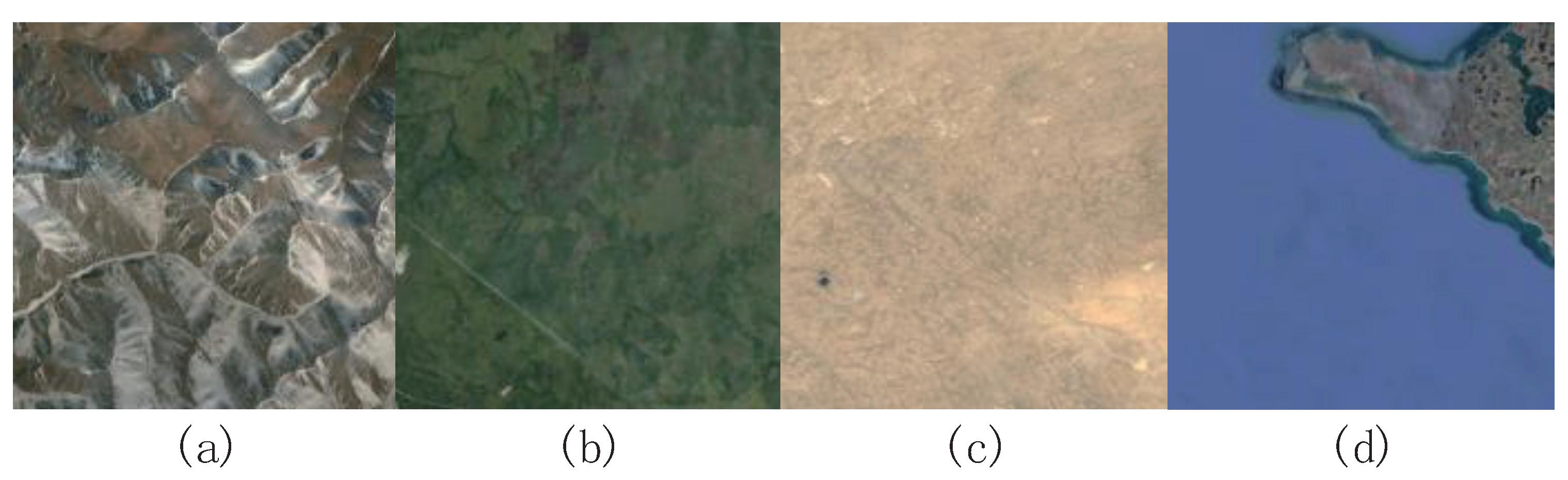
To verify the superiority of IGLL, we conduct experiments on three common datasets: RICE [45], AID [46], and Clear-View [47]. In this section, comparison with the latest state-of-the-art methods validates the applicability and superiority of the IGLL method for RSIs inpainting. Ablation experiments confirm the advantages of the proposed GAM, FFSM, and SVD loss functions. The specific parameters of RICE, AID, and Clear-View datasets are shown in

Table 1. Details of the experimental dataset.

Dataset	Type	Spectrum	Resolution	Image Size	Source	Quantity
RICE [45]	RGB	3	30 m	512 × 512	Google Earth	500
AID [46]	RGB	3	(8–0.5) m	600 × 600	Google Earth	10,000
Clear-View [47]	RGB	3	0.3 m and 0.5 m	1024 × 1024	Landsat	21,080

.

4.1. Datasets

RICE: Lin et al. [45] propose the Remote-sensing Image Cloud removal dataset (RICE). The proposed dataset consists of two parts: RICE1 and RICE2. RICE1 contains 500 pairs of images with a size of 512 × 512. Each pair consists of a cloudy image and a cloudless image. RICE2 contains 450 sets of images with the size of 512 × 512. Each set of RICE2 contains three images, which are the ground truth, the cloudy image, and the mask image, respectively. Figure 4 provides some examples of the RICE dataset.

AID: Xia et al. [46] propose a new large-scale Aerial Image dataset (AID). The dataset includes 30 different scene classes, with approximately 200 to 400 samples, each with a size of 600 × 600 in each class. Figure 5 provides some examples of the AID dataset.

Clear-View: Abhijeet Bhattacharya et al. [47] propose a dataset named Clear-View. This dataset is designed for supervised learning tasks related to reconstructing missing data in remote-sensing images. It contains three types of data noise: (1) salt and pepper noise, caused by transmission errors and analog-to-digital converter errors; (2) the Landsat ETM + scan line corrector (SLC) problem, which is caused by the poor performance of satellite sensors and cross-talk between sensors; (3) thick clouds are present due to poor atmospheric conditions. The dataset contains 21,080 scenes with a size of 1024 × 1024. Each scene contains 3 RGB images with different information. Figure 6 shows some examples of the Clear-View dataset.

4.2. Experimental Details

(1) Training Settings

The model is implemented with the PyTorch (v2.7.1) framework with a single NVIDIA GeForce RTX 3090 GPU. Training procedures are optimized by the Adam optimizer. With reference to the existing work [26], the optimizer parameters are set to $\beta 1=0.5$ and $\beta 2=0.9$ with an initial learning rate of $1\times {10}^{-4}$. The batch size is set to 6. Since the loss function reaches a stable state at around the 40th epoch, the number of total epochs is set to 40 for each dataset. These values are empirically based on the experimental observations in our model.

For our experiments, the mask ratios are set at 10%, 25%, and 77%. This absence of concentrated areas often occurs in RSIs, adding complexity to the inpainting task. Each dataset is shuffled and divided into training and testing sets in a ratio of 4:1. Regions with the size $256\times 256$ are randomly selected to train and test from the corresponding ground truth, noisy image, mask image, and edge image. The dataset encompasses a variety of scenes, effectively validating the IGLL’s generalization capability across diverse scenarios in RSIs.

(2) Evaluation Metrics

The network is evaluated in both qualitative and quantitative aspects. In terms of qualitative evaluation, it is judged whether there are artifacts and whether the structure is restored clearly from the visual perspective. Quantitative evaluation metrics include pixel-level metrics and perceptual-level metrics. Pixel-level metrics include multiscale structural similarity index (MS-SSIM) [48] and peak signal-to-noise ratio (PSNR) [49]. Higher MS-SSIM and PSNR value indicates better results. Although pixel-level evaluation metrics are effective, they still have some limitations. For example, models that perform well on pixel-level metrics may exhibit blurriness. Therefore, it is necessary to use perceptual-level metrics to assess the quality of the result. Perceptual-level metrics include Fréchet inception distance (FID) [50] and learned perceptual image patch similarity (LPIPS) [51] where lower values indicate superior performance.

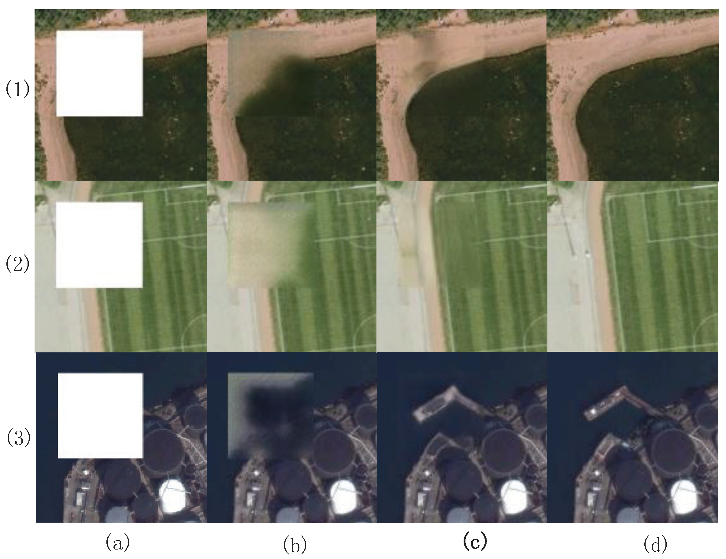
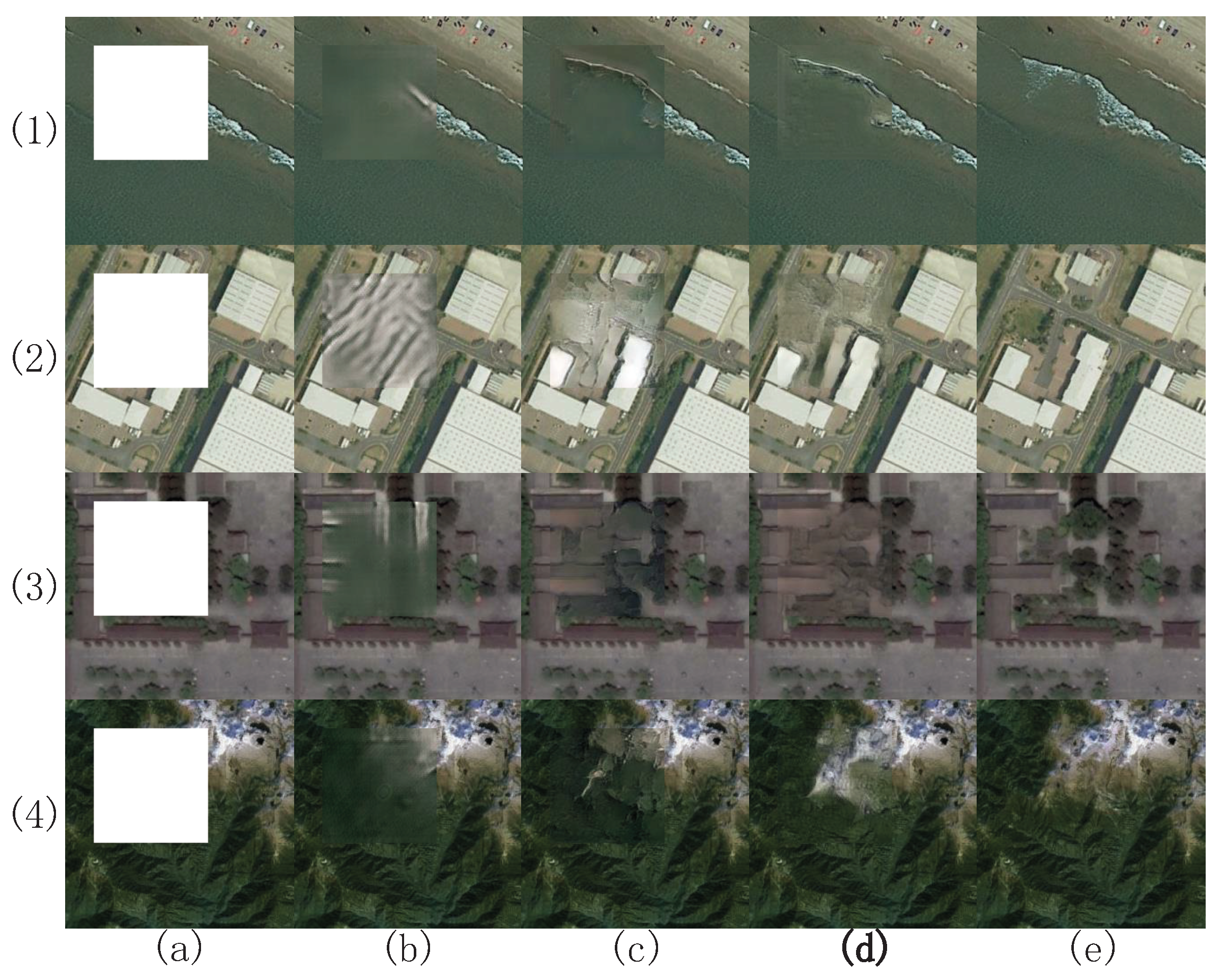
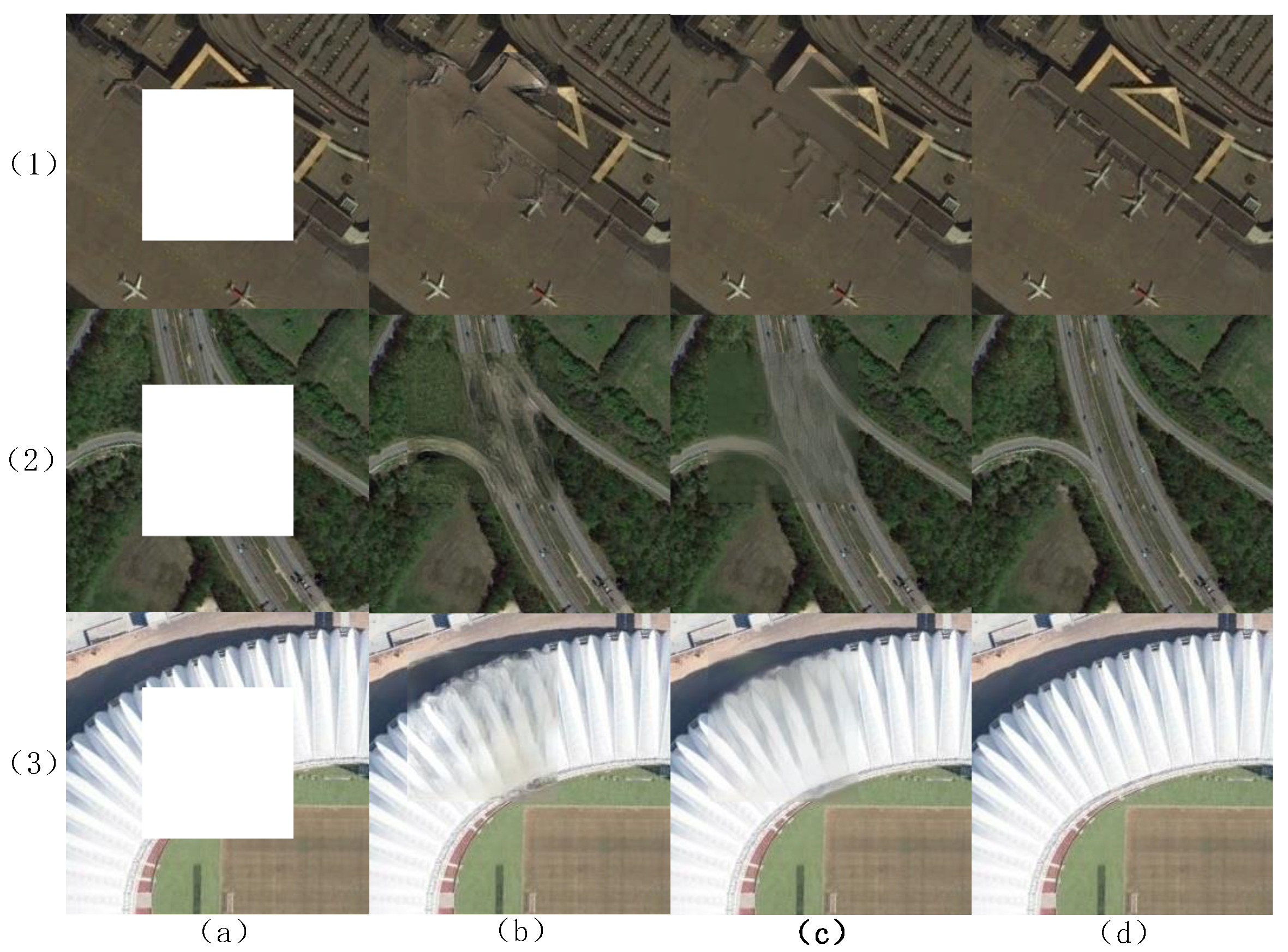
4.3. Inpainting Experiments

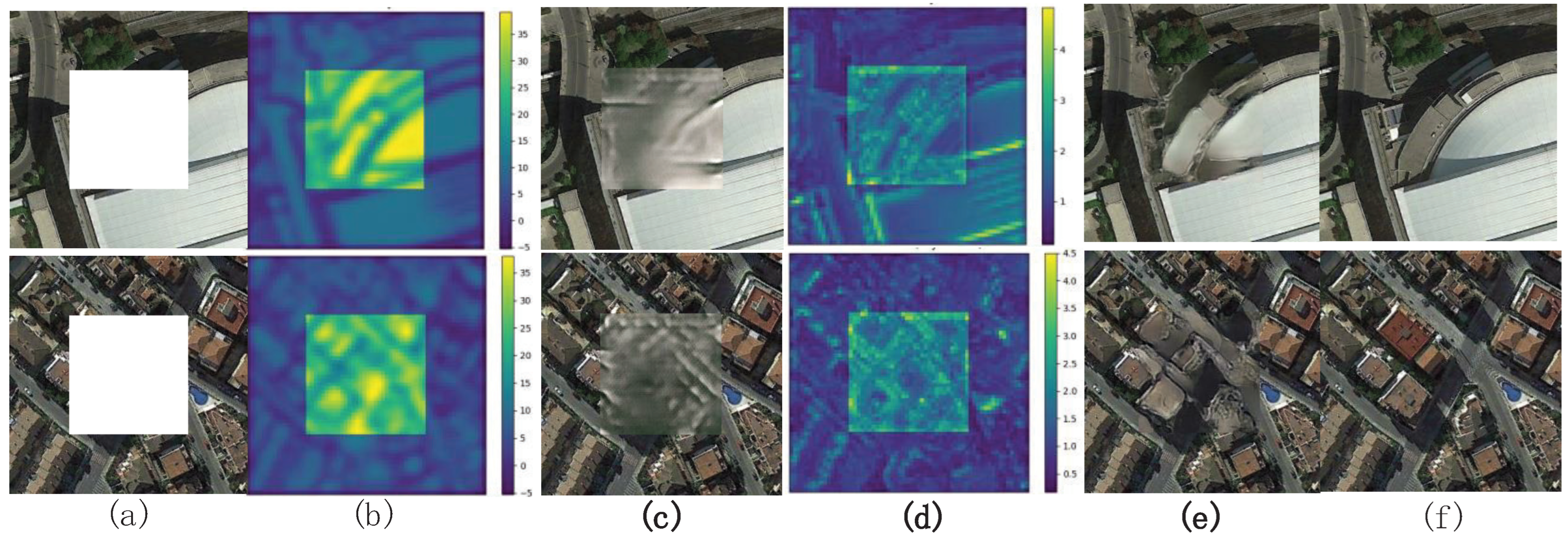
To demonstrate the superiority of IGLL, we compare our IGLL model with state-of-the-art image inpainting lightweight models: DMFN [26], HiFIll [27], HAN [29], and HINT [20]. These models are trained and tested following their optimal configurations described in the respective papers. Some experimental results are shown in Figure 7, and the evaluation metrics are presented in

Table 2. Quantitative comparisons of the proposed IGLL with state-of-the-art inpainting models on three datasets. The best results in each group are highlighted in bold. The ↑ indicates that the larger the value, the better, whereas the ↓ denotes that the smaller the value, the better.

Method	Mask Rate		DMFN [26]	HiFIll [27]	HAN [29]	HINT [20]	Our
MS-SSIM ↑	10%	AID	0.916	0.928	0.937	0.304	0.948
		RICE	0.922	0.931	0.951	0.310	0.952
		Clear-View	0.900	0.905	0.912	0.300	0.933
	25%	AID	0.811	0.830	0.839	0.311	0.865
		RICE	0.821	0.832	0.850	0.312	0.875
		Clear-View	0.772	0.805	0.779	0.301	0.814
	77%	AID	0.711	0.734	0.750	0.324	0.757
		RICE	0.736	0.758	0.760	0.330	0.764
		Clear-View	0.654	0.664	0.722	0.322	0.710
PSNR ↑	10%	AID	27.253	28.330	29.190	16.276	31.621
		RICE	27.359	28.456	29.890	16.290	31.892
		Clear-View	25.890	26.573	27.518	16.001	30.875
	25%	AID	23.003	23.835	24.224	16.409	27.282
		RICE	23.362	23.973	24.633	17.103	31.621
		Clear-View	21.971	22.361	22.258	16.074	27.282
	77%	AID	20.241	21.552	22.031	16.591	21.848
		RICE	21.004	22.217	22.307	16.701	22.925
		Clear-View	20.050	20.383	21.812	16.286	21.578
FID ↓	10%	AID	17.078	18.906	11.911	16.045	6.573
		RICE	16.630	16.758	10.395	16.008	5.298
		Clear-View	18.354	20.083	12.257	16.232	8.252
	25%	AID	58.343	59.951	43.333	28.600	19.554
		RICE	56.247	58.231	42.58	27.560	18.603
		Clear-View	60.000	60.058	45.087	28.973	21.257
	77%	AID	79.092	77.502	77.502	39.343	30.118
		RICE	78.352	77.255	76.281	39.060	29.222
		Clear-View	80.257	79.271	79.354	38.640	33.581
LPIPS ↓	10%	AID	0.088	0.084	0.066	0.445	0.035
		RICE	0.076	0.077	0.051	0.438	0.024
		Clear-View	0.099	0.092	0.089	0.450	0.039
	25%	AID	0.231	0.228	0.178	0.456	0.134
		RICE	0.217	0.199	0.155	0.446	0.126
		Clear-View	0.359	0.282	0.194	0.483	0.136
	77%	AID	0.327	0.323	0.286	0.470	0.177
		RICE	0.259	0.258	0.251	0.379	0.169
		Clear-View	0.389	0.381	0.354	0.493	0.179

. The parameters and GFLOPs for each model are summarized in

Table 3. Comparison of the proposed IGLL with lightweight state-of-the-art methods for the number of parameters. The ↓ denotes that the smaller the value, the less the model’s computational resource consumption. The computational resource consumption of the most lightweight model is denoted in bold.

Method	Param (M) ↓	Gflops (GB) ↓
DMFN [26]	13.036	128.765
HiFIll [27]	9.853	80.307
HAN [29]	19.446	114.737
HINT [20]	21.167	72.940
IGLL	4.458	42.613

.

The experimental results show that the IGLL model is effective and can be generalized to various scenarios. Lightweight convolutional models lack powerful semantic understanding capabilities. They can understand scenes with small variations instead of RSIs with high-information-density. As shown in the first row, when the ground truth information is relatively simple and the mask ratio is low, they all generate satisfactory results without color inconsistency. When dealing with structural variation regions, as shown in the second row, the other models all exhibit significant color deviations. For the complex ground truth information in the third row, the images restored by other models exhibit significant defects in both structure and color. In comparison, IGLL utilizes low rankness to recover images with color consistency. It breaks through local smoothness, maintaining semantic integrity and structural invariance. We also extracted a small amount of data from Google Earth as test data. The trained weights of the model can perform well on untrained self-made data.

The proposed IGLL method demonstrates significant advantages over existing methods in restoring images with large-scale contiguous missing regions. However, in the context of recovering images with small-scale irregular masks, IGLL achieves performance comparable to the SOTA methods. As illustrated in cases (6) and (7), the presence of smaller missing regions and the critical role of residual information in guiding the restoration process of irregular holes substantially reduce the inherent difficulty of the restoration task. Consequently, the performance of all compared methods improves relative to their results on large contiguous missing regions. Specifically, HAN [29] leverages an attention mechanism as its backbone, while HINT [20] employs a transformer structure, both of which endow these methods with superior semantic understanding capabilities compared to CNN-based architectures such as DMFN [26] and HiFill [27]. Thanks to these advanced semantic modeling capabilities, HAN and HINT exhibit superior inpainting performance but at the cost of considerably higher computational overhead. In contrast, the proposed IGLL achieves performance on par with SOTA methods while requiring lower computational overhead, making it particularly suitable for deployment on devices with constrained computational resources.

Regarding quantitative metrics, the proposed IGLL performs well in processing images with different mask ratios and requires less computing cost, as shown in Table 2 and Table 3. When the mask ratio is low, the performance gap between other methods and IGLL is small. As the missing proportion increases, the performance of IGLL surpasses other methods.

4.4. Ablation Study

(1) Verifying the Effectiveness of GAM and FFSM

Ablation experiments are conducted across diverse remote-sensing scenarios by substituting the proposed GAM and FFSM with vanilla attention mechanisms, respectively. From a qualitative evaluation perspective, models without GAM can recover finer details, but they face challenges in dealing with structural deformation and noticeable color inconsistencies, as shown in Figure 8. For example, in case (1), due to the lack of global information understanding, the network may incorrectly select a particular patch for restoration, leading to significant deviations. A model without FFSM possesses limitations in detail recovery. When dealing with images with rich texture details, like case (4), it generates textures with notable differences from the background, due to the lack of specific background patches to provide recovery details. In case (5), the forest occupies a larger area, exhibiting similar smoothness to the river region. Only relying on pixel-level similarity comparison misclassifies the river as part of the forest. On the other hand, only considering semantic-level similarity comparison causes color deviation. Leveraging the advantages of the GAM and FFSM, the proposed IGLL produces optimal results. Introducing background information from multiple granularities enables the algorithm to restore images with complex spatial context. This ensures texture continuity and content fidelity.

The quantitative metrics are shown in

Table 4. Quantitative evaluation for GAM and FFSM. The ↑ indicates that the larger the value, the better, whereas the ↓ denotes that the smaller the value, the better. The result with the best inpainting performance is denoted in bold.

Method	MS-SSIM ↑	PSNR ↑	FID ↓	LPIPS ↓
w/o GAM	0.8463	25.2109	25.3540	0.1333
w/o FFSM	0.8453	25.0450	26.5767	0.1403
w/o structure prior	0.8076	22.2340	92.201	0.2564
w/o position information	0.8453	24.9933	28.8948	0.1435
w/multi-head attention	0.8241	23.4782	67.3224	0.2190
w/o SVD loss	0.8462	25.8886	21.1133	0.1256
IGLL	0.8653	27.2821	19.5542	0.1305

. IGLL outperforms significantly in most metrics. The method with only global attention has poor performance on various metrics. It only compares the correlation of individual pixels and lacks the capability to restore fine details.

(2) Verifying the Effectiveness of Structure Preservation Mechanism

From the perspective of qualitative evaluation, it can be observed that the structure preservation mechanism helps the network recover structurally consistent images, as shown in Figure 9. The lack of structural priors leads to disordered textures in the restored images. When the missing areas are large and concentrated, noticeable repair artifacts occur. From the quantitative metrics, it can be observed that the structural preservation mechanism in IGLL plays a crucial role in enhancing the restoration performance, as shown in Table 4.

(3) Verifying the Effectiveness of the design of GAM

To validate the effectiveness of the GAM, we conduct experiments by using multi-head attention mechanism with three heads. We also conduct ablation experiments by removing the positional information. Some qualitative evaluations are shown in Figure 10 and the quantitative evaluations are shown in Table 4. The visualizations of multi-head attention and single-headed attention are shown in Figure 11. From the qualitative metrics, it is evident that position information enhances the robustness of the network. Since the network stores the spatial information of each pixel, it can leverage contextual features to enhance the stability of the restoration results. The position information significantly improves the continuity of local features and aids in modeling the relevance of global features.

The multi-head attention mechanism is observed to be disadvantageous for preserving the structural characteristics of foreground information. The visualization drawings of head num = 3 and head num = 1 are displayed in Figure 11b,d. Different colors indicate the varying attention scores. The correspondence between values and colors is shown on the right. It is evident that foreground information and background information are more similar in flat areas such as grassland. Since there is a higher correlation between flat areas, the model tends to allocate more attention to flat areas. Multi-head attention leads to excessive local-smoothness in the recovered image and distorted structures in areas with abrupt structural changes. The GAM module employs attention with head = 1, allowing it to balance attention between unsmooth and smooth regions. The proposed GAM can help the method generate basic textures and a reasonable structure.

From the quantitative metrics in Table 4, it is evident that the proposed IGLL achieves the best results at both the pixel-level and perceptual-level. This demonstrates that the proposed GAM module is more suitable for RSI inpainting tasks. Furthermore, combining GAM with other proposed mechanisms can achieve the best image restoration performance.

(4) Verifying the Effectiveness of SVD loss

Experiments are conducted on the AID dataset with and without SVD loss. From the qualitative metrics, as shown in Figure 12, the SVD loss enhances the semantic understanding and maintains color consistency. Besides, the SVD loss ensures the authenticity by constraining the key ranks to be similar. From the quantitative metrics, as illustrated in Table 4, using SVD loss item improves both quantitative and qualitative metrics. The IGLL achieves near-state-of-the-art performance on the LPIPS metric, trailing the top method by merely 0.0049. This marginal discrepancy suggests near-equivalent perceptual quality despite architectural differences.

5. Discussion

The results demonstrate that designing specific network architectures and loss functions based on the intrinsic low-rank and smoothness characteristics of RSIs can restore RSIs with concentrated missing regions under low resource consumption. When recovering RSIs with small-scale missing regions, IGLL and transformer-based methods outperform CNN-based methods, achieving inpainting effects close to the SOTA, as evidenced by the experimental data in (6) and (7) of Figure 7. Notably, as shown in Figure 7(1)–(4), except for our proposed IGLL method, existing studies fail to achieve satisfactory repair results when addressing the task of restoring RSIs with large-area concentrated missing regions. The works [26,27,29] all rely on CNN architectures, which struggle to handle highly challenging inpainting tasks for RSIs with large-scale missing areas. In contrast, the works [20,29] adopt transformer structures, expanding the model’s receptive field and achieving better results. However, these methods consume substantial computational resources and still produce suboptimal inpainting quality for large-scale missing regions. Compared with these mainstream approaches, our model’s effectiveness is validated.

Both the network’s structure and parameters significantly influence performance. As for structure, removing the learnable edges from the IGLL generator deprives the network of redundant weights to capture and reconstruct structural mutation information, failing to maintain structural consistency. Additionally, our experiments reveal that the results are influenced by mask information, indicating that the integration of mask information at both the initial information injection stage and the intermediate processing stage can facilitate the model’s more effective recovery of underlying data. It is a foundational understanding in the image inpainting field—articulated in numerous existing works [52,53]—that introducing mask information at the initial input stage aids model restoration. Our designed GAM module demonstrates that incorporating mask partition information during the intermediate model processing phase similarly also enhances the model’s capacity to recover missing data efficiently. This highlights the extended utility of mask guidance beyond the input stage, showing its multi-stage efficacy in optimizing inpainting performance. As for parameters, our model exhibits high sensitivity to loss function hyperparameters and learning rates. Extensive testing confirmed that the hyperparameters reported in this paper enable the IGLL model to achieve optimal RSI inpainting results.

The proposed IGLL still has limitations: limited scalability and a complex parameter tuning process. The scalability of this approach requires further investigation, particularly its generalizability to multi-source data environments. Multi-source data often exhibit heterogeneous characteristics (e.g., varying modalities and sampling rates), which may challenge the method’s robustness. For instance, in remote-sensing applications, integrating optical imagery, synthetic aperture radar (SAR) data, and LiDAR point clouds requires the method to adapt to distinct radiation characteristics.

6. Conclusions

In this paper, we propose an RSI inpainting GAN method combining low-rankness and local smoothness (IGLL). The IGLL integrates the RSIs intrinsic characteristics with the deep-learning method. To boost the color consistency of the restoration results, the proposed GAM, FFSM, and SVD loss item obey low-rankness characteristic. The proposed GAM and FFSM introduce pixel-level and semantic-level repetitive features to fill the unknown regions, enhancing the spatial coherence and spatial realism. The SVD loss enforces rank consistency by constraining the similarity of singular value distributions across regions, avoiding color shift. Besides, the structure preservation mechanism obeys local-smoothness characteristic to preserve the structural coherence of extensive missing areas. IGLL outperforms existing state-of-the-art models in terms of speed and restoration effectiveness, recovering the RSIs with high mask ratio. This method is limited by mask accuracy. In the future, a self-supervised blind inpainting method with efficient prior should be developed to overcome these limitations.

References

1. Zhang, Y.; Rossow, W.B.; Lacis, A.A.; Oinas, V.; Mishchenko, M.I. Calculation of radiative fluxes from the surface to top of atmosphere based on ISCCP and other global data sets: Refinements of the radiative transfer model and the input data. J. Geophys. Res. Atmos. 2004, 109, D19105. [Google Scholar] [CrossRef]
2. Wang, Y. DMDiff: A Dual-Branch Multimodal Conditional Guided Diffusion Model for Cloud Removal Through SAR-Optical Data Fusion. Remote Sens. 2025, 17, 965. [Google Scholar]
3. Du, Y.; He, J.; Huang, Q.; Sheng, Q.; Tian, G. A Coarse-to-Fine Deep Generative Model with Spatial Semantic Attention for High-Resolution Remote Sensing Image Inpainting. IEEE Trans. Geosci. Remote Sens. 2022, 60, 5621913. [Google Scholar] [CrossRef]
4. Palejwala, S.K.; Skoch, J.; Lemole, G.M., Jr. Removal of symptomatic craniofacial titanium hardware following craniotomy: Case series and review. Interdiscip. Neurosurg. 2015, 2, 115–119. [Google Scholar] [CrossRef]
5. Sun, H.; Ma, J.; Guo, Q.; Zou, Q.; Song, S.; Lin, Y.; Yu, H. Coarse-to-fine task-driven inpainting for geoscience images. IEEE Trans. Circuits Syst. Video Technol. 2023, 33, 7170–7182. [Google Scholar] [CrossRef]
6. Karwowska, K.; Wierzbicki, D.; Kedzierski, M. Image Inpainting and Digital Camouflage: Methods, Applications, and Perspectives for Remote Sensing. IEEE J. Sel. Top. Appl. Earth Obs. Remote Sens. 2025, 18, 8215–8247. [Google Scholar] [CrossRef]
7. Zhang, Y.; Tu, Z.; Lu, J.; Xu, C.; Shen, L. Fusion of low-rankness and smoothness under learnable nonlinear transformation for tensor completion. Knowl.-Based Syst. 2024, 296, 111917. [Google Scholar] [CrossRef]
8. Wang, H.; Peng, J.; Qin, W.; Wang, J.; Meng, D. Guaranteed tensor recovery fused low-rankness and smoothness. IEEE Trans. Pattern Anal. Mach. Intell. 2023, 45, 10990–11007. [Google Scholar] [CrossRef]
9. Zha, Z.; Wen, B.; Yuan, X.; Zhou, J.; Zhu, C.; Kot, A.C. Low-rankness guided group sparse representation for image restoration. IEEE Trans. Neural Netw. Learn. Syst. 2022, 34, 7593–7607. [Google Scholar] [CrossRef]
10. Kohler, M.; Langer, S. Statistical theory for image classification using deep convolutional neural network with cross-entropy loss under the hierarchical max-pooling model. J. Stat. Plan. Inference 2025, 234, 106188. [Google Scholar] [CrossRef]
11. Ružić, T.; Pižurica, A. Context-aware patch-based image inpainting using Markov random field modeling. IEEE Trans. Image Process. 2014, 24, 444–456. [Google Scholar] [CrossRef]
12. Cao, R.; Chen, Y.; Chen, J.; Zhu, X.; Shen, M. Thick cloud removal in Landsat images based on autoregression of Landsat time-series data. Remote Sens. Environ. 2020, 249, 112001. [Google Scholar] [CrossRef]
13. Chen, J.; Zhu, X.; Vogelmann, J.E.; Gao, F.; Jin, S. A simple and effective method for filling gaps in Landsat ETM+ SLC-off images. Remote Sens. Environ. 2011, 115, 1053–1064. [Google Scholar] [CrossRef]
14. Wong, R.; Zhang, Z.; Wang, Y.; Chen, F.; Zeng, D. HSI-IPNet: Hyperspectral imagery inpainting by deep learning with adaptive spectral extraction. IEEE J. Sel. Top. Appl. Earth Obs. Remote Sens. 2020, 13, 4369–4380. [Google Scholar] [CrossRef]
15. Wan, Z.; Zhang, J.; Chen, D.; Liao, J. High-fidelity pluralistic image completion with transformers. In Proceedings of the IEEE/CVF International Conference on Computer Vision, Montreal, QC, Canada, 10–17 October 2021; pp. 4692–4701. [Google Scholar]
16. Pathak, D.; Krahenbuhl, P.; Donahue, J.; Darrell, T.; Efros, A.A. Context encoders: Feature learning by inpainting. In Proceedings of the IEEE Conference on Computer Vision and Pattern Recognition, Las Vegas, NV, USA, 27–30 June 2016; pp. 2536–2544. [Google Scholar]
17. Dong, Q.; Cao, C.; Fu, Y. Incremental transformer structure enhanced image inpainting with masking positional encoding. In Proceedings of the IEEE/CVF Conference on Computer Vision and Pattern Recognition, New Orleans, LA, USA, 18–24 June 2022; pp. 11358–11368. [Google Scholar]
18. He, K.; Chen, X.; Xie, S.; Li, Y.; Dollár, P.; Girshick, R. Masked autoencoders are scalable vision learners. In Proceedings of the IEEE/CVF Conference on Computer Vision and Pattern Recognition, New Orleans, LA, USA, 18–24 June 2022; pp. 16000–16009. [Google Scholar]
19. Vaswani, A.; Shazeer, N.; Parmar, N.; Uszkoreit, J.; Jones, L.; Gomez, A.N.; Kaiser, Ł.; Polosukhin, I. Attention is all you need. In Proceedings of the Advances in Neural Information Processing Systems, Long Beach, CA, USA, 4–9 December 2017; Volume 30. [Google Scholar]
20. Chen, S.; Atapour-Abarghouei, A.; Shum, H.P. HINT: High-quality INpainting Transformer with Mask-Aware Encoding and Enhanced Attention. IEEE Trans. Multimed. 2024, 26, 7649–7660. [Google Scholar] [CrossRef]
21. Zeng, Y.; Fu, J.; Chao, H.; Guo, B. Aggregated contextual transformations for high-resolution image inpainting. IEEE Trans. Vis. Comput. Graph. 2023, 29, 3266–3280. [Google Scholar] [CrossRef] [PubMed]
22. Li, W.; Lin, Z.; Zhou, K.; Qi, L.; Wang, Y.; Jia, J. Mat: Mask-aware transformer for large hole image inpainting. In Proceedings of the IEEE/CVF Conference on Computer Vision and Pattern Recognition, New Orleans, LA, USA, 18–24 June 2022; pp. 10758–10768. [Google Scholar]
23. Panboonyuen, T.; Charoenphon, C.; Satirapod, C. SatDiff: A Stable Diffusion Framework for Inpainting Very High-Resolution Satellite Imagery. IEEE Access 2025, 13, 51617–51631. [Google Scholar] [CrossRef]
24. Khanna, S.; Liu, P.; Zhou, L.; Meng, C.; Rombach, R.; Burke, M.; Lobell, D.; Ermon, S. Diffusionsat: A generative foundation model for satellite imagery. arXiv 2023, arXiv:2312.03606. [Google Scholar]
25. Dong, J.; Yin, R.; Sun, X.; Li, Q.; Yang, Y.; Qin, X. Inpainting of remote sensing SST images with deep convolutional generative adversarial network. IEEE Geosci. Remote. Sens. Lett. 2019, 16, 173–177. [Google Scholar] [CrossRef]
26. Hui, Z.; Li, J.; Wang, X.; Gao, X. Image fine-grained inpainting. arXiv 2020, arXiv:2002.02609. [Google Scholar]
27. Yi, Z.; Tang, Q.; Azizi, S.; Jang, D.; Xu, Z. Contextual residual aggregation for ultra high-resolution image inpainting. In Proceedings of the IEEE/CVF Conference on Computer Vision and Pattern Recognition, Seattle, WA, USA, 13–19 June 2020; pp. 7505–7517. [Google Scholar]
28. Wang, N.; Zhang, Y.; Zhang, L. Dynamic selection network for image inpainting. IEEE Trans. Image Process. 2021, 30, 1784–1798. [Google Scholar] [CrossRef] [PubMed]
29. Deng, Y.; Hui, S.; Meng, R.; Zhou, S.; Wang, J. Hourglass Attention Network for Image Inpainting. In Computer Vision—ECCV 2022, Proceedings of the European Conference on Computer Vision, Tel Aviv, Israel, 23–27 October 2022; Springer: Berlin/Heidelberg, Germany, 2022; pp. 483–501. [Google Scholar]
30. Wang, N.; Ma, S.; Li, J.; Zhang, Y.; Zhang, L. Multistage attention network for image inpainting. Pattern Recognit. 2020, 106, 107448. [Google Scholar] [CrossRef]
31. Song, J.; Meng, C.; Ermon, S. Denoising diffusion implicit models. arXiv 2020, arXiv:2010.02502. [Google Scholar]
32. Song, Y.; Ermon, S. Improved techniques for training score-based generative models. In Proceedings of the Advances in Neural Information Processing Systems, Virtual, 6–12 October 2020; Volume 33, pp. 12438–12448. [Google Scholar]
33. Ettari, A.; Nappa, A.; Quartulli, M.; Azpiroz, I.; Longo, G. Adaptation of Diffusion Models for Remote Sensing Imagery. In Proceedings of the IGARSS 2024-2024 IEEE International Geoscience and Remote Sensing Symposium, Athens, Greece, 7–12 July 2024; pp. 7240–7243. [Google Scholar]
34. Rombach, R.; Blattmann, A.; Lorenz, D.; Esser, P.; Ommer, B. High-resolution image synthesis with latent diffusion models. In Proceedings of the IEEE/CVF Conference on Computer Vision and Pattern Recognition, New Orleans, LA, USA, 18–24 June 2022; pp. 10684–10695. [Google Scholar]
35. Su, Z.; Liu, W.; Yu, Z.; Hu, D.; Liao, Q.; Tian, Q.; Pietikäinen, M.; Liu, L. Pixel difference networks for efficient edge detection. In Proceedings of the IEEE/CVF International Conference on Computer Vision, Montreal, BC, Canada, 11–17 October 2021; pp. 5117–5127. [Google Scholar]
36. Devlin, J.; Chang, M.W.; Lee, K.; Toutanova, K. BERT: Pre-training of Deep Bidirectional Transformers for Language Understanding. In Proceedings of the Conference of the North American Chapter of the Association for Computational Linguistics: Human Language Technologies, vol. 6. long and short papers: Conference of the North American Chapter of the Association for Computational Linguistics: Human Language Technologies (NAACL HLT 2019), Minneapolis, MN, USA, 2–7 June 2019. [Google Scholar]
37. Gatys, L.A.; Ecker, A.S.; Bethge, M. Image style transfer using convolutional neural networks. In Proceedings of the IEEE Conference on Computer Vision and Pattern Recognition, Las Vegas, NV, USA, 27–30 June 2016; pp. 2414–2423. [Google Scholar]
38. Gatys, L.A.; Ecker, A.S.; Bethge, M. A neural algorithm of artistic style. arXiv 2015, arXiv:1508.06576. [Google Scholar] [CrossRef]
39. Wang, C.; Xu, C.; Wang, C.; Tao, D. Perceptual adversarial networks for image-to-image transformation. IEEE Trans. Image Process. 2018, 27, 4066–4079. [Google Scholar] [CrossRef]
40. Wang, X.; Yu, K.; Wu, S.; Gu, J.; Liu, Y.; Dong, C.; Qiao, Y.; Change Loy, C. Esrgan: Enhanced super-resolution generative adversarial networks. In Proceedings of the European Conference on Computer Vision (ECCV) Workshops, Munich, Germany, 8–14 September 2018. [Google Scholar]
41. Simonyan, K.; Zisserman, A. Very deep convolutional networks for large-scale image recognition. arXiv 2014, arXiv:1409.1556. [Google Scholar]
42. Kilmer, M.E.; Martin, C.D. Factorization strategies for third-order tensors. Linear Algebra Its Appl. 2011, 435, 641–658. [Google Scholar] [CrossRef]
43. Struski, L.; Morkisz, P.; Trzcinski, B.T. Efficient GPU implementation of randomized SVD and its applications. Expert Syst. Appl. 2024, 248, 123462. [Google Scholar] [CrossRef]
44. Farnia, F.; Ozdaglar, A. Do GANs always have Nash equilibria? In Proceedings of the International Conference on Machine Learning, Virtual, 13–18 July 2020; pp. 3029–3039. [Google Scholar]
45. Lin, D.; Xu, G.; Wang, X.; Wang, Y.; Sun, X.; Fu, K. A remote sensing image dataset for cloud removal. arXiv 2019, arXiv:1901.00600. [Google Scholar]
46. Xia, G.S.; Hu, J.; Hu, F.; Shi, B.; Bai, X.; Zhong, Y.; Zhang, L.; Lu, X. AID: A benchmark data set for performance evaluation of aerial scene classification. IEEE Trans. Geosci. Remote. Sens. 2017, 55, 3965–3981. [Google Scholar] [CrossRef]
47. Bhattacharya, A.; Baweja, T. Clear-view: A dataset for missing data in remote sensing images. In Proceedings of the 2021 IEEE 19th World Symposium on Applied Machine Intelligence and Informatics (SAMI), Herl’any, Slovakia, 21–23 January 2021; pp. 000077–000082. [Google Scholar]
48. Wang, Z.; Simoncelli, E.P.; Bovik, A.C. Multiscale structural similarity for image quality assessment. In Proceedings of the Thrity-Seventh Asilomar Conference on Signals, Systems & Computers, Pacific Grove, CA, USA, 9–12 November 2003; Volume 2, pp. 1398–1402. [Google Scholar]
49. Eskicioglu, A.M.; Fisher, P.S. Image quality measures and their performance. IEEE Trans. Commun. 1995, 43, 2959–2965. [Google Scholar] [CrossRef]
50. Heusel, M.; Ramsauer, H.; Unterthiner, T.; Nessler, B.; Hochreiter, S. Gans trained by a two time-scale update rule converge to a local nash equilibrium. In Proceedings of the Advances in Neural Information Processing Systems, Long Beach, CA, USA, 4–9 December 2017; Volume 30. [Google Scholar]
51. Zhang, R.; Isola, P.; Efros, A.A.; Shechtman, E.; Wang, O. The unreasonable effectiveness of deep features as a perceptual metric. In Proceedings of the IEEE Conference on Computer Vision and Pattern Recognition, Salt Lake City, UT, USA, 18–23 June 2018; pp. 586–595. [Google Scholar]
52. Sun, S.; Zhao, B.; Mateen, M.; Chen, X.; Wen, J. Mask guided diverse face image synthesis. Front. Comput. Sci. 2022, 16, 163311. [Google Scholar] [CrossRef]
53. Fang, Z.; Lin, H.; Xu, X. Mask-guided model for seismic data denoising. IEEE Geosci. Remote. Sens. Lett. 2022, 19, 8026705. [Google Scholar] [CrossRef]
Figure 1. The architecture of the proposed IGLL. IGLL is a generative adversarial network (GAN). (1) As for architecture, the proposed global attention module (GAM) and flexible feature similarity module (FFSM) are incorporated in generator. Additionally, structural priors are introduced into both the discriminator and generator. (2) As for optimization process, a singular value decomposition (SVD) loss is added to the generator loss function. The generator is jointly guided by the loss function of the generator and the discriminator. To achieve the balance between the generator and the discriminator, the SVD loss item is also added to the discriminator loss. To minimize the value of the loss function, the SVD loss is added only to the discriminator loss items that are likely to be judged as real.
Remotesensing 17 02132 g001
Figure 2. Structure of the global attention module (GAM).
Remotesensing 17 02132 g002
Figure 3. Structure of the flexible feature similarity module(FFSM).
Remotesensing 17 02132 g003
Figure 4. Examples of RICE dataset. (a) Mountain. (b) Meadow. (c) Desert. (d) Sea.
Remotesensing 17 02132 g004
Figure 5. Examples of AID dataset. (a) Bare land. (b) Baseball field. (c) Beach. (d) Commercial. (e) Park.
Remotesensing 17 02132 g005
Figure 6. Examples of Clear-View dataset. (1) Noisy image. (2) Mask. (3) Label. (a) Images with salt and pepper noise. (b) Line corrector. (c) Clouds.
Remotesensing 17 02132 g006
Figure 7. Qualitative comparisons on images (256 × 256) to verify the effectiveness of the IGLL. From left to right: (a) masked image; (b) DFMN; (c) HiFIll; (d) HAN; (e) HINT; (f) IGLL; (g) ground truth. Best results in each group are highlighted in bold. Each number corresponds to a distinct example, and the white regions signify the areas requiring repair.
Remotesensing 17 02132 g007
Figure 8. Qualitative comparisons on images (256 × 256) of AID [46] to verify the effectiveness of the GAM and FFSM. From left to right: (a) masked images; (b) w/o GAM; (c) w/o FFSM; (d) IGLL; (e) ground truth. Each number corresponds to a distinct example, and the white regions signify the areas requiring repair. The result with the best inpainting performance is denoted in bold.
Remotesensing 17 02132 g008
Figure 9. Qualitative comparisons on images (256 × 256) of AID to verify the effectiveness of the structural preservation mechanism. From left to right: (a) masked image; (b) without structure retention; (c) with structure retention; (d) ground truth. Each number corresponds to a distinct example, and the white regions signify the areas requiring repair. The result with the best inpainting performance is denoted in bold.
Remotesensing 17 02132 g009
Figure 10. Qualitative comparisons on images (256 × 256) of AID [46] to verify the effectiveness of the GAM. From left to right: (a) masked image; (b) using multi-head; (c) without position information; (d) IGLL; (e) ground truth. Each number corresponds to a distinct example, and the white regions signify the areas requiring repair. The result with the best inpainting performance is denoted in bold.
Remotesensing 17 02132 g010
Figure 11. Visual comparisons on images (256 × 256) of AID [46] to verify the effectiveness of the GAM and FFSM. From left to right: (a) masked image; (b) attention heatmap produced by using head num = 3; (c) result produced by using head num = 1; (d) attention heatmaps produced by using head num = 1; (e) results produced by using head num = 1; (f) ground truth. The white regions signify the areas requiring repair.The result with the best inpainting performance is denoted in bold.
Remotesensing 17 02132 g011
Figure 12. Ablation study results for the SVD Loss. Models trained with and without the SVD Loss are compared. The inclusion of the SVD Loss significantly enhances performance. (a) Masked image. (b) Without SVD loss. (c) Ours. (d) Ground truth. Each number corresponds to a distinct example, and the white regions signify the areas requiring repair. The result with the best inpainting performance is denoted in bold.
Remotesensing 17 02132 g012