NGSTGAN: N-Gram Swin Transformer and Multi-Attention U-Net Discriminator for Efficient Multi-Spectral Remote Sensing Image Super-Resolution

Abstract

The reconstruction of high-resolution (HR) remote sensing images (RSIs) from low-resolution (LR) counterparts is a critical task in remote sensing image super-resolution (RSISR). Recent advancements in convolutional neural networks (CNNs) and Transformers have significantly improved RSISR performance due to their capabilities in local feature extraction and global modeling. However, several limitations remain, including the underutilization of multi-scale features in RSIs, the limited receptive field of Swin Transformer’s window self-attention (WSA), and the computational complexity of existing methods. To address these issues, this paper introduces the NGSTGAN model, which employs an N-Gram Swin Transformer as the generator and a multi-attention U-Net as the discriminator. The discriminator enhances attention to multi-scale key features through the addition of channel, spatial, and pixel attention (CSPA) modules, while the generator utilizes an improved shallow feature extraction (ISFE) module to extract multi-scale and multi-directional features, enhancing the capture of complex textures and details. The N-Gram concept is introduced to expand the receptive field of Swin Transformer, and sliding window self-attention (S-WSA) is employed to facilitate interaction between neighboring windows. Additionally, channel-reducing group convolution (CRGC) is used to reduce the number of parameters and computational complexity. A cross-sensor multispectral dataset combining Landsat-8 (L8) and Sentinel-2 (S2) is constructed for the resolution enhancement of L8’s blue (B), green (G), red (R), and near-infrared (NIR) bands from 30 m to 10 m. Experiments show that NGSTGAN outperforms the state-of-the-art (SOTA) method, achieving improvements of 0.5180 dB in the peak signal-to-noise ratio (PSNR) and 0.0153 in the structural similarity index measure (SSIM) over the second best method, offering a more effective solution to the task.

1. Introduction

In the past few decades, the rapid development of satellite technology has led to a significant increase in the volume of RSIs, with applications spanning disaster monitoring [1,2], agriculture [3], weather forecasting [4], target detection [5], and land use classification [6,7]. HR images, in particular, offer richer texture information, which is crucial for detailed surface feature extraction and interpretation in downstream tasks, thereby enhancing the accuracy of applications. Although image SR does not increase the physical resolution of the imaging sensor, it can effectively reconstruct high-frequency details from existing image data, enabling more informative representations than traditional enhancement methods. Therefore, SR has emerged as a promising solution for the extraction of richer information from RSIs without increasing hardware costs. Early methods include pan-sharpening [8] and interpolation [9], which, while simple and efficient, often suffer from smoothing and blurring issues. Other methods, such as reconstruction-based approaches [10,11], sparse representation [12], and convex projection [13], offer strong theoretical support but are complex and require substantial a priori knowledge, limiting their widespread application in remote sensing image processing across different sensors.

The rapid advancement of information technology has led to the widespread adoption of deep learning-based methods across various fields, including SR image processing. CNNs [14] have garnered significant attention in the field of computer vision due to their advantages in automatic feature extraction, parameter sharing, spatial structure preservation, translation invariance, and generalization ability. The seminal work by Dong et al. [15], which applied CNNs to image SR for the first time, marked a significant milestone, outperforming traditional methods and validating the feasibility of CNNs in this domain. Building upon the success of SRCNN, Dong et al. [16] proposed FSRCNN, which introduced a novel tail-up sampling training technique, establishing it as a dominant training method for image SR. However, both SRCNN and FSRCNN were limited to only three convolutional layers, which constrained their depth. The advent of residual networks [17] propelled the development of deep learning models towards greater depths. VDSR [18], for instance, utilized 20 layers of convolution and achieved element-wise summation of the input image and model output feature maps through residual connections, effectively mitigating the issue of gradient vanishing in deep models. Its performance surpassed that of SRCNN. Subsequently, the performance of CNN-based models progressively advanced to deeper levels [19,20,21], although increasing model depth is not without its limitations. Researchers began to incorporate attention mechanisms into image SR. RCAN [22] combined the channel attention mechanism with VDSR to construct the first SR network based on attention, demonstrating that attention mechanisms can significantly enhance the performance of SR models. Following this, second-order attention [23], residual attention [24], and pixel attention [25] were employed to further enhance the performance of image SR models. Today, attention mechanisms and residual structures have become standard components in SR models. Moreover, CNNs have been introduced to SR processing of RSIs. RSIs, unlike ordinary optical images, are characterized by complex feature types and significant scale differences [26]. Leveraging these characteristics, LGCNet [27] outperformed SRCNN by learning multi-level representations of local details and global environments, becoming the first network specifically designed for the SR of RSIs. Lei et al. [28] built upon LGCNet and, by incorporating the multi-scale self-similarity of RSIs, proposed HSENet, which has become a classical model for RSISR. To further enhance the effectiveness of RSISR, researchers have continuously improved the network structure and proposed various new attention mechanisms [29,30] that significantly improve the quality of generated images. However, the local characteristics of CNNs limit their ability to model the global pixel dependencies in RSIs, which affects their performance in the SR task for RSIs.

Despite the substantial advancements in CNNs for image SR, many of these methods primarily focus on minimizing absolute pixel errors, often resulting in a high peak signal-to-noise ratio (PSNR) but images that appear overly smooth and lack perceptual quality. To overcome these limitations, generative adversarial networks (GANs), as detailed in [31,32,33], have been proposed. GANs consist of two opposing networks: the generator and the discriminator, trained in a zero-sum game. The generator aims to create realistic images to fool the discriminator, while the discriminator’s task is to differentiate between real and generated images. Through this adversarial training, GANs generate images that exhibit superior perceptual quality compared to those produced by traditional CNN-based methods. SRGAN [31], the pioneering network to apply GANs to image SR, features a generator consisting of multiple stacked residual blocks and a discriminator based on a VGG-style convolutional neural network. SRGAN introduces a novel loss function that utilizes a pre-trained VGG network to extract image features, optimizing the feature distance between generated and real samples to enhance perceptual similarity. However, the use of perceptual loss can sometimes introduce artifacts. To mitigate this issue, ESRGAN [32] improves upon SRGAN by employing dense residual blocks and removing the batch normalization layer, which reduces artifacts. Despite these improvements, the use of dense residual blocks increases computational resource consumption, potentially affecting ESRGAN’s efficiency. Applying a typical optical image super-resolution GAN model directly to RSIs may lead to feature blurring and texture loss in the generated images. Researchers have made various advancements in GANs for RSISR, including edge sharpening [34], the introduction of attention mechanisms [35], gradient referencing [36], and leveraging the unique characteristics of RSIs [37]. These improvements often focus on optimizing the generator. As research continues, some scholars have shifted their focus to optimizing the discriminator. For instance, Wei et al. [38] proposed a multi-scale U-Net discriminator with attention, which captures structural features of images at multiple scales and generates more realistic high-resolution images. Similarly, Wang et al. [39] introduced a vision Transformer (ViT) discriminator, which also captures structural features at multiple scales and has achieved notable results. Despite these advancements, GAN-based methods still rely on CNN architectures for the construction of the generator and discriminator, and they fall short of fully addressing the inherent localization limitations of CNNs.

The Transformer architecture [40] was first applied to the field of natural language processing (NLP), and Dosovitskiy et al. [41] innovatively introduced it into the field of computer vision (CV) by proposing the ViT. ViT has achieved SOTA performance in several CV tasks. ViT directly models the global dependencies of an image through the self-attention mechanism, which outperforms the local convolution operation of CNNs in processing global features, especially in large-scale datasets. However, the computational complexity of the multi-head self-attention (MHSA) mechanism in ViT is quadratic with respect to the length of the input sequence, which consumes significant computational resources when processing large images. To reduce the computational complexity of MHSA, the Swin Transformer [42] introduces a shift window, limiting the MHSA computation to non-overlapping localized windows. This modification makes the computational complexity linearly related to the image size while still allowing for the interaction of information across the windows, effectively improving computational efficiency. SwinIR [43] combines the localized feature extraction capability of CNNs with the global modeling capability of Transformers. The model includes a shallow feature extraction module, a deep feature extraction module, and an HR reconstruction module. The deep feature extraction module consists of multiple layers of Swin Transformer with residual connections. This structure has become a mainstream design in Transformer-based SR methods. SRFormer [44] introduces a replacement attention mechanism in the Transformer, which not only improves the resolution of the image but also effectively reduces the computational burden while retaining details. TransENet [45] is the first Transformer model applied to the SR of RSIs. However, it upsamples the feature maps before decoding, leading to high computational resource consumption and complexity. To tackle token redundancy and limited multi-scale representation in large-area remote sensing super-resolution, TTST [46] introduces a Transformer that selectively retains key tokens, enriches multi-scale features, and leverages global context, achieving better performance with reduced computational cost. CSCT [47] proposes a channel–spatial coherent Transformer that enhances structural detail and edge reconstruction through spatial–channel attention and frequency-aware modeling, aiming to overcome the limitations of CNN- and GAN-based RSISR methods. SWCGAN [48] integrates CNNs and Swin Transformers in both the generator and discriminator and demonstrates improved perceptual quality compared to earlier CNN-based GANs. However, despite their advantages, these Transformer-based methods still face challenges such as high memory consumption and computational overhead during training, particularly in the deep feature extraction stages. While Swin Transformer improves efficiency using shifted window mechanisms, the limited receptive field within each window may restrict the model’s ability to capture long-range dependencies across wide spatial extents—an essential requirement in remote sensing tasks. In contrast, our proposed NGSTGAN explicitly addresses these limitations by introducing a lightweight and efficient N-Gram-based shifted window self-attention mechanism that enhances the model’s capacity to capture both local structures and global dependencies without significantly increasing computational complexity. Moreover, the ISFE module further strengthens spatial structure preservation by facilitating interaction-based enhancement across features. Compared to TTST, CSCT, and SWCGAN, NGSTGAN strikes a better balance between structural fidelity, perceptual quality, and computational efficiency, which is crucial for scalable deployment in large-area RSISR applications.

In language modeling (LM), an N-Gram [49] is a set of consecutive sequences of characters or words, widely used in the field of NLP as a probabilistic, statistics-based language model, where the value of N is usually set to 2 or 3 [49]. The N-Gram model performed well in early statistical approaches because it could take into account longer context spans in sentences. Even in some deep learning-based LMs, the N-Gram concept is still employed. Sent2Vec [50] learns N-Gram embeddings using sentence embeddings. To better learn sentence representations, the model proposed in [51] uses recurrent neural networks (RNNs) to compute the context of word N-Grams and passes the results to the attention layer. Meanwhile, some high-level vision studies have also adopted this concept. For example, pixel N-Grams [52] apply N-Grams at the pixel level, both horizontally and vertically, and view N-Gram networks [53] treat successive multi-view images of three-dimensional objects along time steps as N-Grams. Unlike these, this paper builds on previous N-Gram language models. 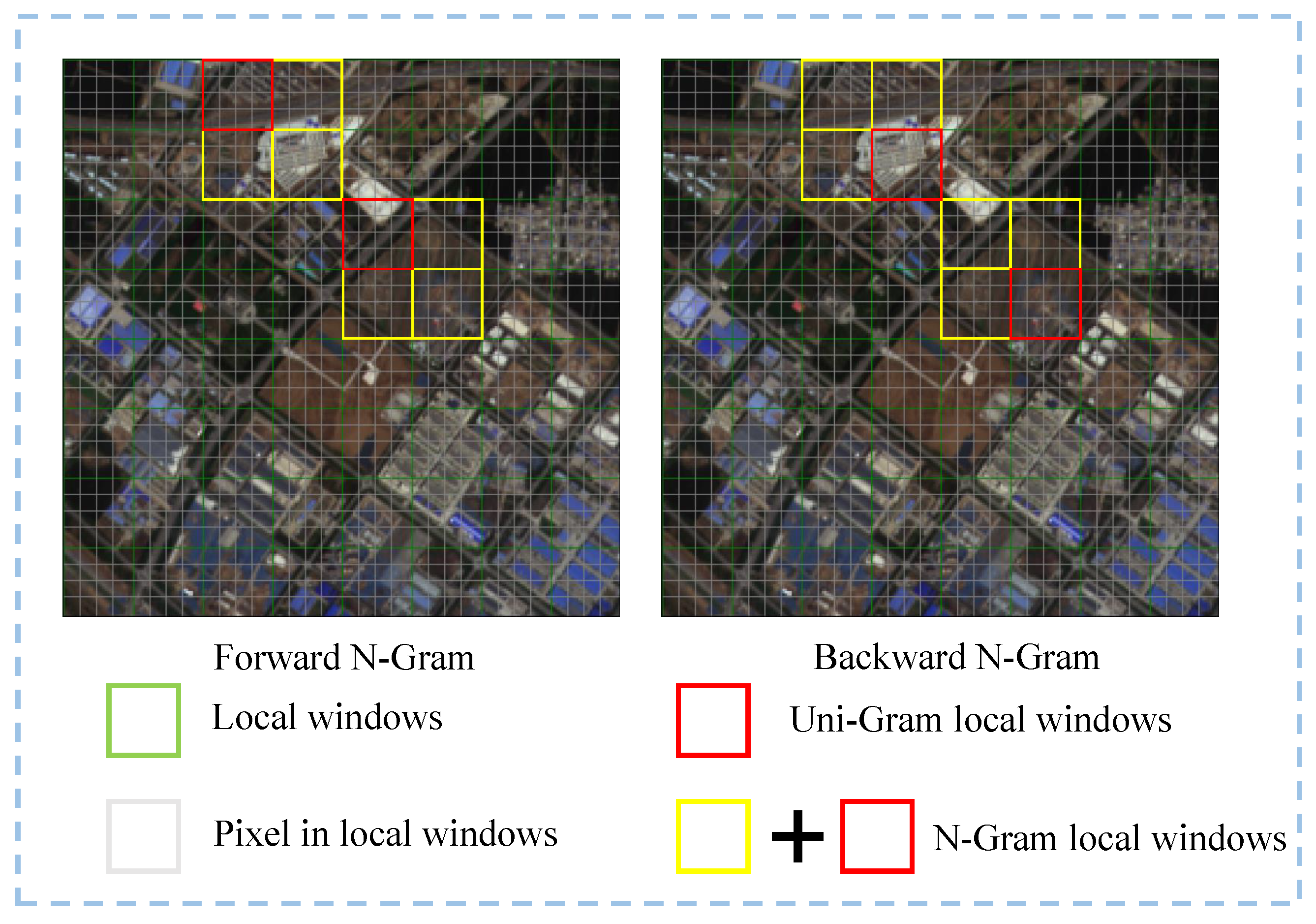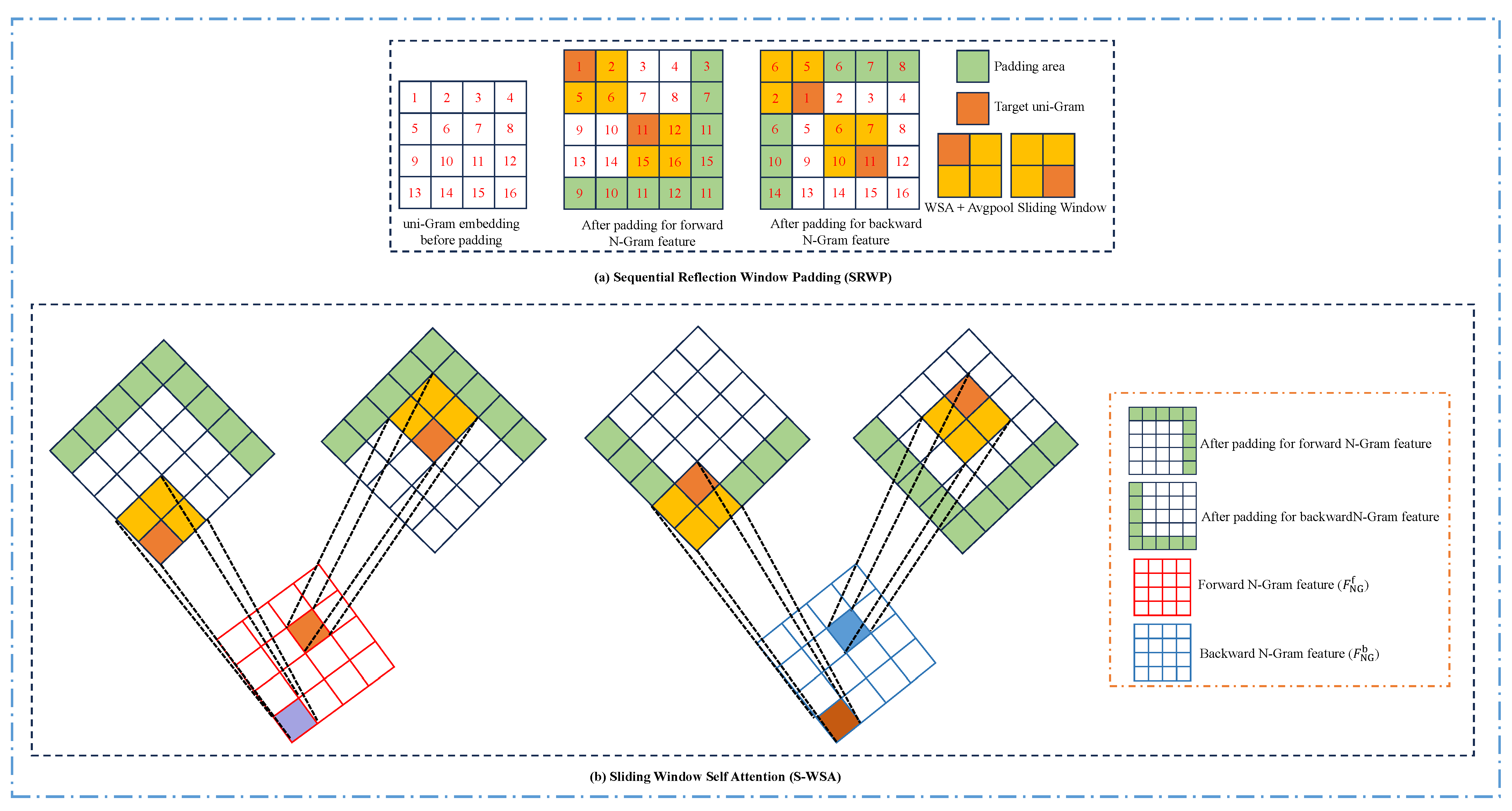Referring to NGSwin [54], the concept of N-Grams is introduced into image processing, focusing on bidirectional two-dimensional information at the local window level. This approach offers a new method for processing single RSIs in low-level visual tasks.

To summarize, current RSISR models face three major limitations. First, RSIs often contain multiple ground objects with strong self-similarity and repeated patterns across different spatial scales. However, most existing methods fail to effectively exploit the inherent multi-scale characteristics of RSIs. Second, the commonly used WSA in Swin Transformer is limited to local windows, making it difficult to leverage texture cues from adjacent regions. The independent and sequential sliding windows further restrict the model’s ability to capture global contextual dependencies. Third, many state-of-the-art RSISR models rely on heavy architectures with high computational cost. It is therefore essential to design lightweight models that not only limit parameters to 1 M∼4 M but also reduce the total number of multiply–accumulate operations during inference [55,56].

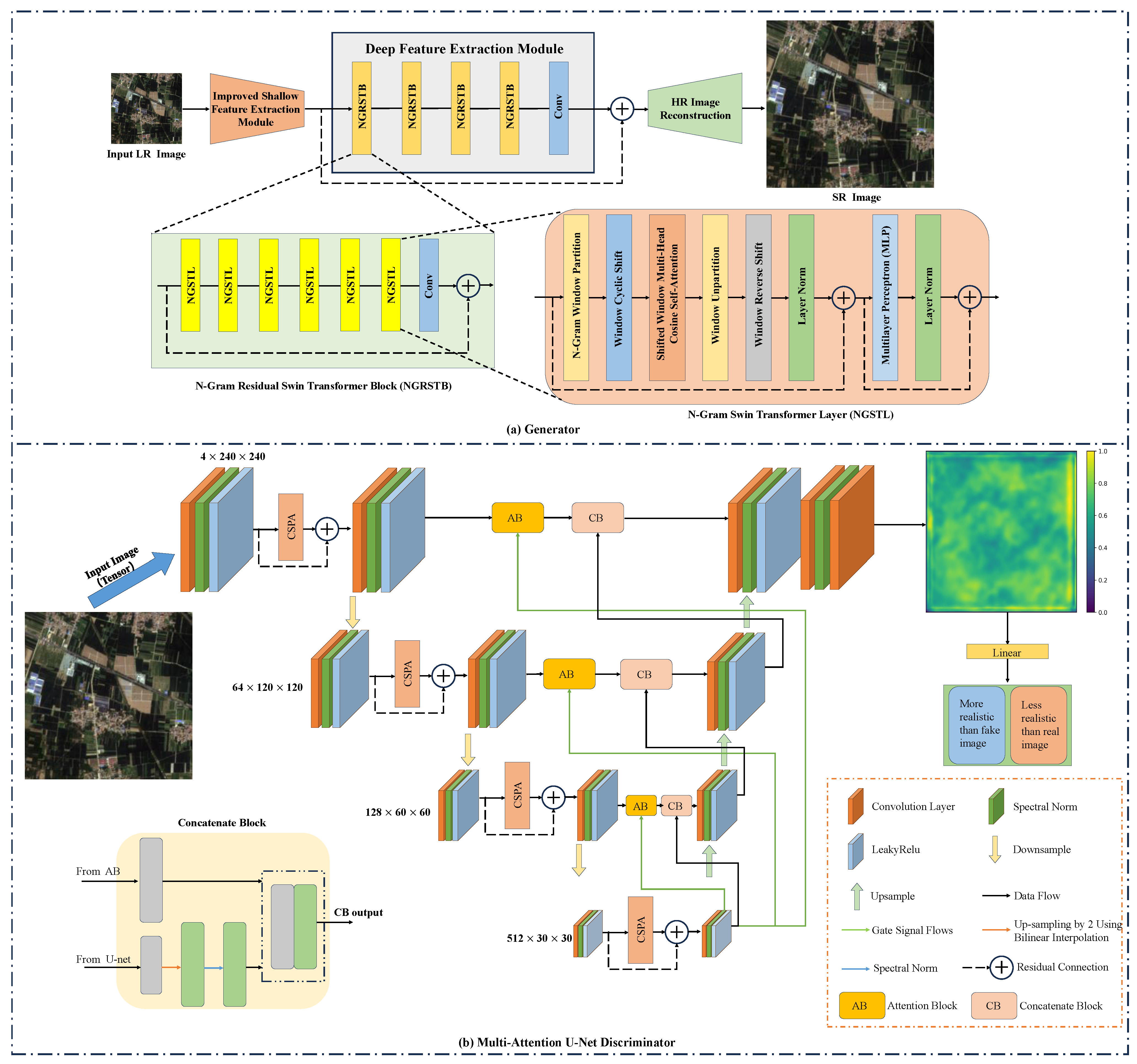
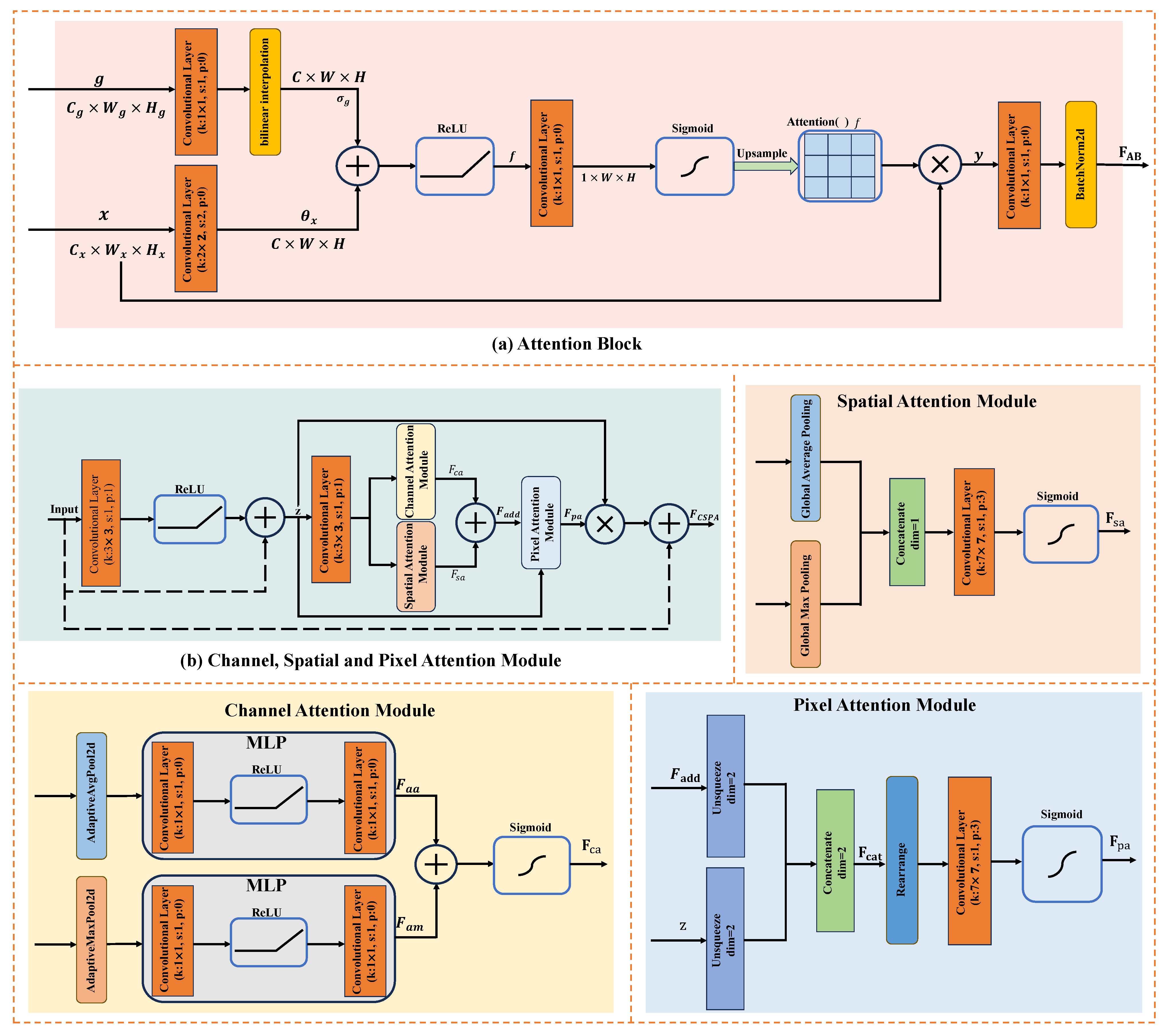
This study aims to enhance the spatial resolution of LR RSIs using deep learning techniques, thereby producing high-quality data for remote sensing applications. To achieve this, this study proposes a new RSISR model, namely NGSTGAN. It integrates the N-Gram Swin Transformer as the generator and combines the multi-attention U-Net as the discriminator. To tackle the multi-scale characteristics of remote sensing imagery, this study proposes a multi-attention U-Net discriminator, which is an extension of the attention U-Net [38] and incorporates channel, spatial, and pixel attention modules before downsampling. The U-Net structure provides pixel-wise feedback to the generator, facilitating the generation of more detailed features. It also enhances feature extraction capabilities [57] by integrating information from various scales through multi-level feature extraction and skip connections. The channel attention module enhances the representation of feature maps at each layer, enabling the generator to concentrate on critical channels, which is particularly important for complex remote sensing image features such as texture and color. The spatial attention module efficiently identifies significant regions and improves the spatial detail performance of U-Net in reconstructing high-resolution images, allowing the model to focus on specific feature regions and accurately recover details. Conversely, the pixel attention module offers robust feature representation at the local pixel level, making U-Net more adaptable and flexible in processing fine image information, such as feature edges and small details. Additionally, to extract multi-scale and multi-directional features from the input image, enrich the feature expression, and enhance the model’s ability to capture complex texture and detail information, the ISFE is designed in the generator, achieving promising results. 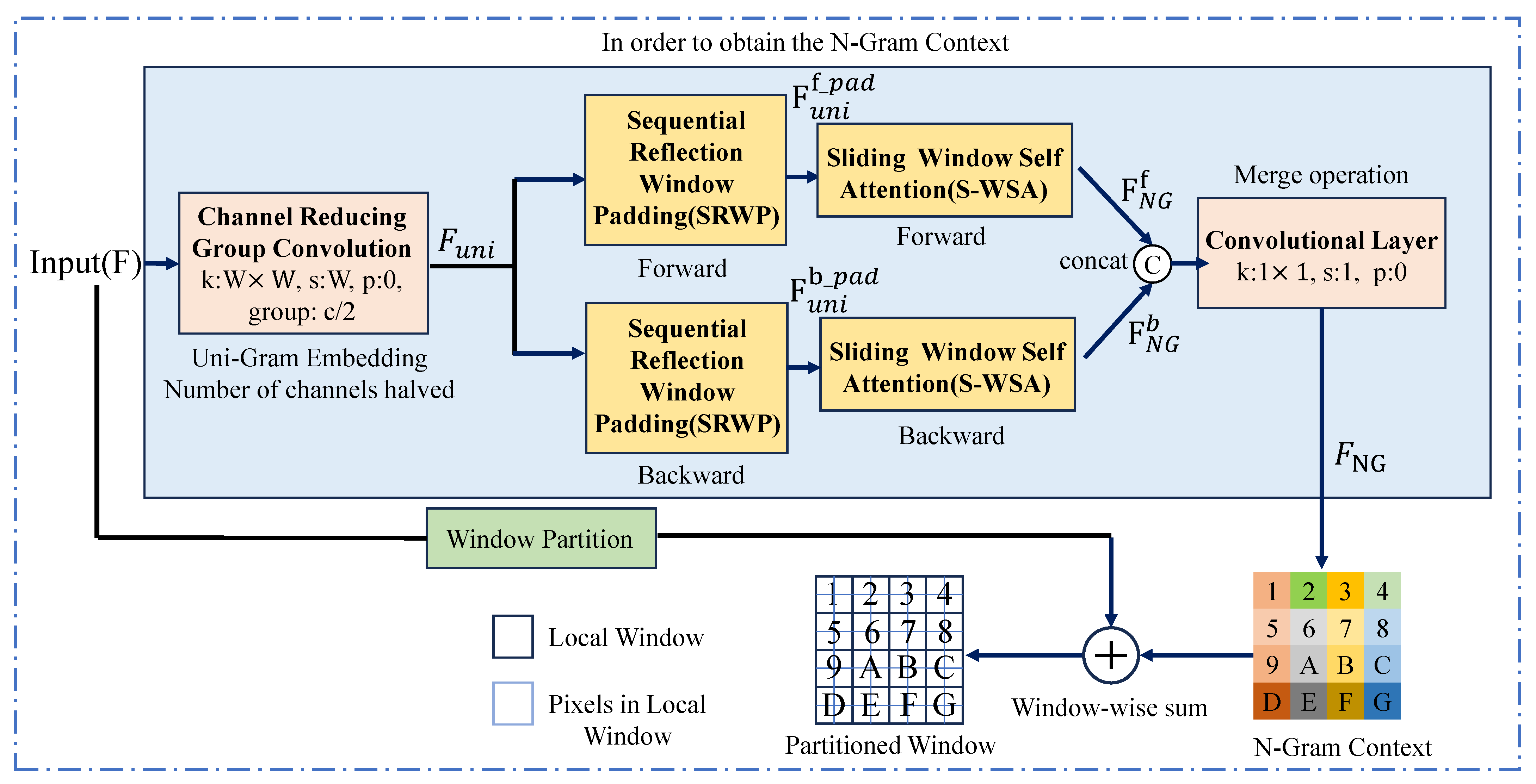To address the limitation of the Swin Transformer’s limited receptive field, where degraded pixels cannot be recovered by utilizing the information of neighboring windows, we refer to NGSwin [54] and introduce the N-Gram concept into the Swin Transformer. Through the S-WSA method, neighboring uni-Gram embeddings are able to interact with each other, allowing N-Gram contextual features to be generated before window segmentation and enabling the full utilization of neighboring window information to recover degraded pixels. The specifics of the N-Gram implementation are detailed in Section 2.3.2. To reduce the number of parameters and the complexity of the model, we employ a CRGC method [54,58] to simplify the N-Gram interaction process.

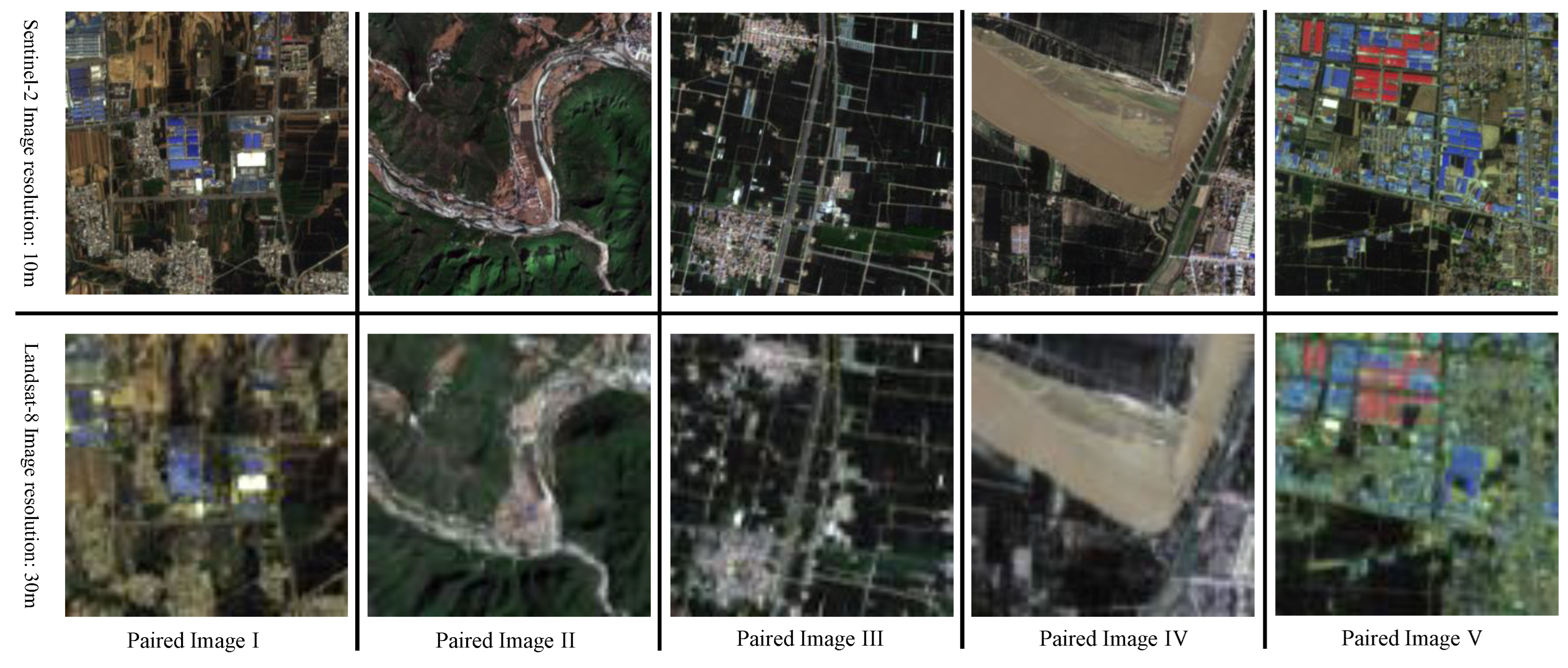
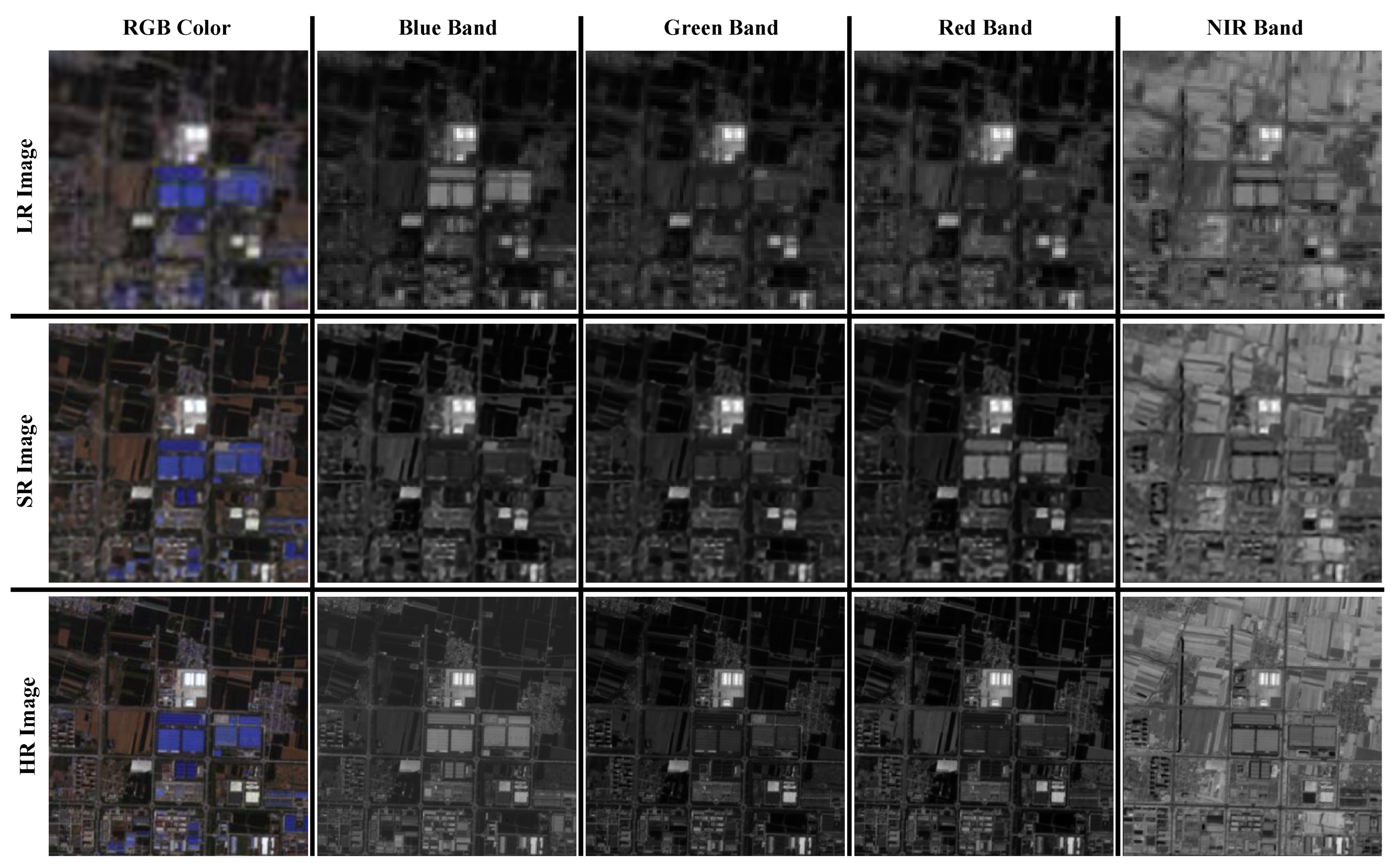
Currently, most RSISR studies primarily rely on RGB-band datasets, which are widely used due to their availability and ease of visualization. However, for many real-world applications such as land use classification, crop monitoring, and environmental assessment, multispectral data can provide more comprehensive and accurate information. Recent studies have highlighted the value of multispectral Landsat imagery in various remote sensing tasks beyond RGB, including cloud removal and missing data recovery. For example, spatiotemporal neural networks have been used to effectively remove thick clouds from multi-temporal Landsat images [59], while tempo-spectral models have demonstrated strong performance in reconstructing missing data across time series of Landsat observations [60]. These works underscore the growing importance of leveraging multi-band satellite data to enhance the performance of downstream remote sensing tasks. To broaden the application scope of super-resolved imagery, this study introduces a novel SR dataset composed of multi-band remote sensing images derived from publicly available L8 and S2 sources. Unlike most existing RSISR datasets limited to RGB, our dataset includes the NIR band, enabling super-resolution processing on four bands: R, G, B, and NIR. The proposed method is capable of handling this multi-band input, expanding the potential applications of SR-enhanced imagery in multispectral analysis scenarios.

The primary contributions of this paper are summarized as follows:

(1)

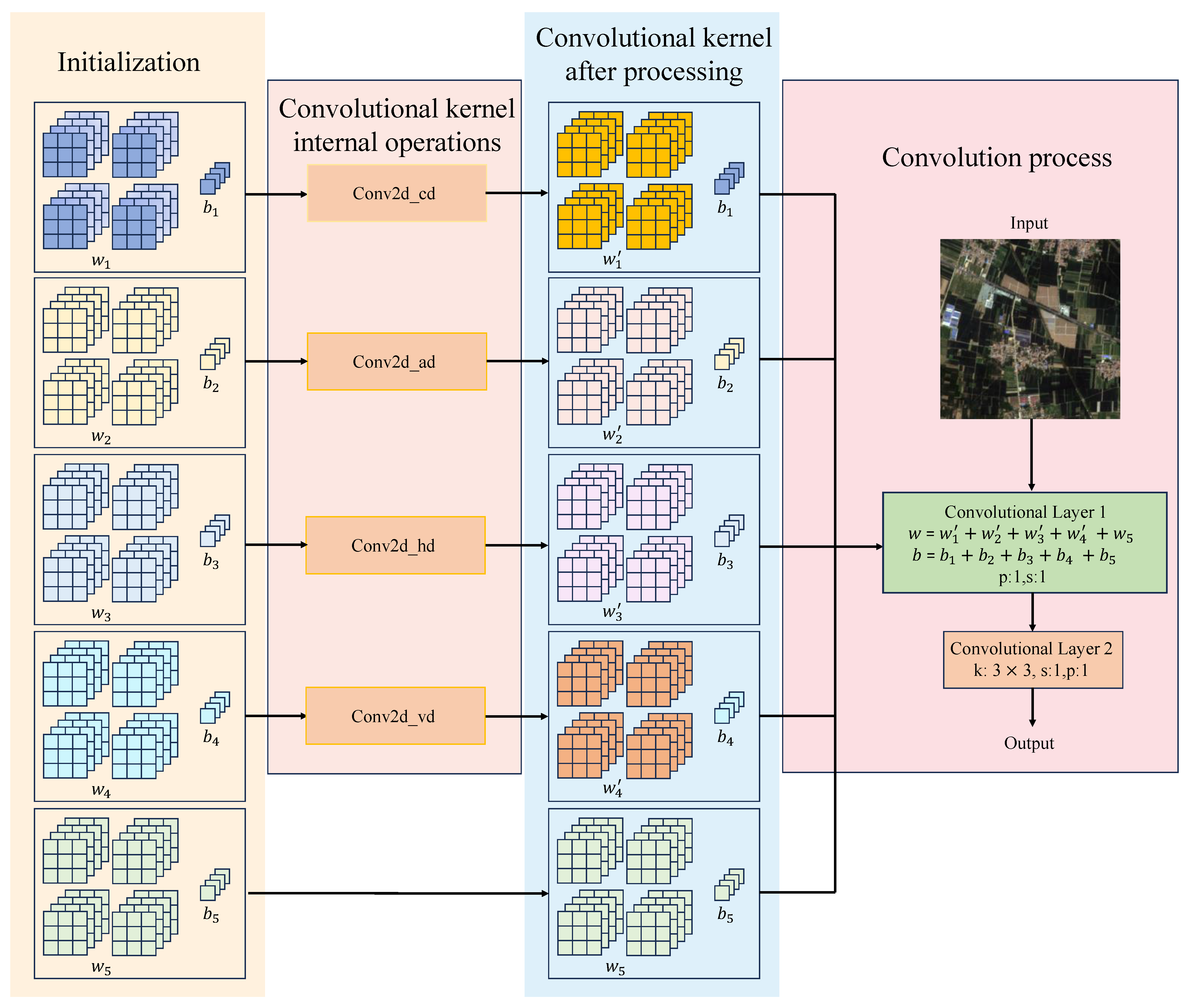
An ISFE is proposed to extract multi-scale and multi-directional features by combining different convolutional kernel parameters, thereby enhancing the model’s ability to capture complex texture and detail information, specifically designed for multispectral RSIs.

(2)

The N-Gram concept is introduced into Swin Transformer, and the N-Gram window partition is proposed, which significantly reduces the number of parameters and computational complexity.

(3)

The multi-attention U-Net discriminator is proposed by adding spatial, channel, and pixel attention mechanisms to the attention U-Net discriminator, which improves the accuracy of detail recovery and reduces information loss in SR tasks, ultimately enhancing image quality.

(4)

A custom multi-band remote sensing image dataset is constructed to further verify the wide applicability and excellent performance of NGSTGAN in the SR task for multispectral images.

This paper is structured as follows. Section 2 presents the method proposed in this study, Section 3 describes the datasets and experimental setup, Section 4 provides both quantitative and qualitative analyses of the experimental results, Section 5 discusses the findings, and Section 6 concludes the paper with a summary of the key findings.

2. Methods

2.1. Definition of N-Gram in Images

As illustrated in Figure 1, N-Gram language models utilize consecutive sequences of forward, backward, or bidirectional words as N-Grams to predict target words [50]. In contrast to models that do not employ N-Grams, where words are often treated as independent entities, the inclusion of contextual features necessitates the introduction of RNNs, attention mechanisms, or average word embeddings. In the N-Gram model, text is segmented into sequences of N words, with each N-Gram treated as a separate feature. Upon recognizing an N-Gram as a feature, it is typically considered independently, without direct interaction with or combination with other N-Gram sequences.

In the image, we define the non-overlapping local window in the Swin Transformer as the uni-Gram, within which each pixel interacts with every other pixel through a self-attention mechanism. The N-Gram is a larger window that contains the uni-Gram and its neighboring windows. Each uni-Gram in the image and each pixel within the uni-Gram in the N-Gram are analogous to a word and its character in text, respectively. As shown in Figure 2, with N set to 2, the red frame delineates the local uni-Gram window, while the yellow frame highlights its neighboring local uni-Gram window. Together, the red and yellow areas form the local N-Gram window. The local windows in the lower right (or upper left) corners of the graph are designated as forward (or backward) N-Gram neighbors. The interaction between N-Grams will be elaborated upon in “N-Gram Window Partition” subsection of Section 2.3.2.

To illustrate the expansion of the model’s receptive field through the application of N-Gram concepts, consider an input image subjected to a single-layer convolution operation with a $k\times k$ convolutional kernel, a stride of s, and a padding of p. The receptive field (R) of the single-layer convolution can be calculated using the following equation:

$$R=k+2p$$

(1)

For a multilayer convolution, the receptive field is initially $R_1=k+2p$ for the first layer and subsequently $R_2=R_1+(k-1)\times s$ for the second layer. More generally, the receptive field of the l-th layer can be recursively expressed as follows:

$$R_l=R_{l-1}+(k-1)\times s$$

(2)

If the N-Gram mechanism is employed after each layer of convolution to integrate the context (i.e., the information of neighboring windows) at each position, let w denote the window size and n denote the size of the N-Gram. For computational convenience, we consider only the information of the neighboring windows before and after the current window for both the forward and backward N-Gram mechanisms. The receptive fields of the forward and backward N-Grams are calculated using the same formula, which can be uniformly expressed as follows:

$$R_{\mathrm{n}\_\mathrm{gram}}=w+2p+(n-1)\times (w+2p-s)$$

(3)

To more intuitively demonstrate the effect of the N-Gram mechanism on the expansion of the receptive field, we set $w=3$, $k=3$, $s=2$, $p=1$, and $n=2$. This configuration yields a receptive field of $R=k+2p=3+2\times 1=5$ for the single-layer window. The receptive fields for the forward and backward N-Grams are $R_{\mathrm{fwd}\_\mathrm{ngram}}=R_{\mathrm{bwd}\_\mathrm{ngram}}=3+2\times 1+(2-1)\times (3+2\times 1-2)=8$, respectively. Thus, the sum of the receptive fields of the forward and backward N-Grams is 16. By incorporating the forward and backward N-Gram mechanisms, the receptive field is extended from 5 to 16, significantly enhancing the model’s ability to capture contextual information and, thus, improving the perceptual quality.

2.2. Overall Architecture of the Model

Figure 3 illustrates the overall architecture of the NGSTGAN model proposed by this study, which comprises two primary components: the generator and the discriminator. The generator includes three components: the ISFE, the deep feature extraction module (DFEM), and the HR image reconstruction module. Inspired by NGSwin [54], the N-Gram concept is introduced in the RSTB of DFEM [43] to form the NGRSTB. Additionally, drawing inspiration from A-ESRGAN [38], the discriminator adopts the improved attention U-Net. The main structure is based on U-Net, with the addition of the CSPA, which is applied before each downsampling step to enhance feature representation at different levels. The training configuration for the generator in NGSTGAN is provided in

Table 1. Training configuration of the NGSTGAN generator.

	N-Grams	Depth	Heads	Ended Dim	Window_Size	Patch_Size	Norm_Layer	Act_Layer
Generator	2	(6, 6, 6, 6)	(6, 6, 6, 6)	96	8	1	LayerNorm	GELU

. Each module is described in detail below.

2.3. Generator

2.3.1. Improved Shallow Feature Extraction Module

Given the following training dataset: ${[I_i^{\mathrm{LR}}\in {\mathbb{R}}^{C_{in}\times H\times W},I_i^{\mathrm{HR}}\in {\mathbb{R}}^{C_{in}\times H_r\times W_r}]}_{i=1}^n$, where $C_{in}$ denotes the number of bands of the input image, H and W denote the height and width of the LR image, $H_r$ and $W_r$ denote the height and width of the HR image, and r denotes the SR times. In the training set, an LR image ($I^{\mathrm{LR}}$) and its corresponding HR image ($I^{\mathrm{HR}}$) are selected. First, the input LR image ($I^{\mathrm{LR}}$) is mapped to a higher dimensional feature space by ISFE. Unlike the traditional shallow feature extraction [43], which only uses a single 2D convolutional layer to extract features, ISFE combines multiple convolutional operations, and through the combination of multiple convolutional kernel parameters, it is capable of extracting multi-scale and multi-directional features from the input image, aiming at enriching the feature representation and enhancing the model’s ability to capture the complex texture and detail information. The specific structure of ISFE is shown in Figure 4. The initial stage of ISFE needs to initialize five convolution kernels with weights and biases ($[w_1,w_2,w_3,w_4,w_5]$ and $[b_1,b_2,b_3,b_4,b_5]$, respectively). In Conv2d_cd, the convolution kernel is flattened, and the fifth element (with subscripts starting at 0) is subtracted from the sum of the other elements to achieve the effect of a high-pass filter, which ultimately returns the updated weights and bias. The formula is expressed as follows:

$$w_1^{\prime }[:,:,4]=w_1[:,:,4]-\sum _{i=1}^8{w}_1[:,:,i].$$

(4)

The structure of Conv2d_ad is similar to that of Conv2d_cd, with the addition of the $\theta$ parameter, which is used to rearrange the elements of the convolution kernel and weight them in a predetermined order. This approach enhances the model’s ability to extract multi-scale and multi-directional feature information, particularly when processing complex multi-spectral RSIs, thereby improving the model’s texture and detail capture capabilities. The adjustment of each element in the convolution kernel can be expressed by the following equation:

$$w_2^{\prime }=w_2-\theta ·w_2[:,:,[3,0,1,6,4,2,7,8,5]],$$

(5)

where $w_2^{\prime }$ denotes the weights of the convolution kernel returned after the Conv2d_ad weight update.

The Conv2d_hd operation involves copying the elements from the first column (i.e., elements 0, 3, and 6) of the original convolution kernel to the first column of the new tensor. The third column (elements 2, 5, and 8) of the new tensor is then filled with the negative values of the corresponding elements from the original convolution kernel. The Conv2d_vd operation follows a similar approach, but it operates on different elements of the convolution kernel. It copies the elements from the first row (i.e., elements 0, 1, and 2) of the original convolution kernel to the first row of the new tensor and fills the third row (elements 6, 7, and 8) with the negative values of the corresponding elements from the original convolution kernel. The formulas for adjusting the elements in the convolution kernel for Conv2d_hd and Conv2d_vd are provided in Equations (6) and (7), respectively.

$$w_3^{\prime }=\left\{\begin{array}{c}{w}_3^{\prime }[:,:,i],i=0,3,6;\hfill \\ -w_3^{\prime }[:,:,i].i=2,5,8.\hfill \end{array}\right.$$

(6)

$$w_4^{\prime }=\left\{\begin{array}{c}{w}_4^{\prime }[:,:,i],i=0,1,2;\hfill \\ -w_4^{\prime }[:,:,i].i=6,7,8.\hfill \end{array}\right.$$

(7)

In the context of the proposed methodology, $w_3^{\prime }$ and $w_4^{\prime }$ represent the updated weights of the convolution kernels following the adjustments to the weights of Conv2d_hd and Conv2d_vd, respectively. The weights ($w_5$) of the convolution kernel are left unchanged, preserving their original values. Similarly, the biases $[b_1,b_2,b_3,b_4,b_5]$ remain unaltered, as they are not subject to the aforementioned modifications. Subsequently, the combined weights and biases of the convolution kernels, after all the operations have been performed, are aggregated to form the new weights and biases of the convolution kernel for convolutional layer 1, as calculated below:

$$\begin{array}{cc}\hfill w& =w_1^{\prime }+w_2^{\prime }+w_3^{\prime }+w_4^{\prime }+w_5,\hfill \\ \hfill b& =b_1+b_2+b_3+b_4+b_5.\hfill \end{array}$$

(8)

Subsequently, the low-resolution image ($I^{LR}$) is sequentially fed into convolutional layer 1 and convolutional layer 2 to yield the output of the ISFE. The operation of the ISFE is denoted as $H_{\mathrm{ISFE}}(·)$, and the extracted features are represented as $F_0\in {\mathbb{R}}^{C\times H\times W}$, where C denotes the number of feature channels. Thus, the entire process of the ISFE can be succinctly encapsulated as follows:

$$F_0=H_{\mathrm{ISFE}}\left(I^{\mathrm{LR}}\right).$$

(9)

The implementation of ISFE primarily relies on convolutional operations, which are adept at processing early visual information. This characteristic facilitates more stable optimization and enhances the quality of the outcomes, as previously noted in [45]. Moreover, ISFE offers a straightforward approach to mapping the input image space into a higher dimensional feature space.

2.3.2. Deep Feature Extraction Module

As illustrated in Figure 3a, the DFEM is primarily composed of K NGRSTBs and a $3\times 3$ convolutional layer. Specifically, the intermediate features ($F_1,F_2,\dots ,F_K$) and the DFEM output features ($F_{\mathrm{DFEM}}$) are extracted sequentially as follows:

$$F_i=H_{{\mathrm{NGRSTB}}_i}\left(F_{i-1}\right),i=1,2,\dots ,K$$

(10)

$$F_{\mathrm{DFEM}}=H_{\mathrm{Conv}}\left(F_K\right),$$

(11)

where $H_{{\mathrm{NGRSTB}}_i}$ represents the i-th NGRSTB and $H_{\mathrm{Conv}}$ denotes the final convolutional layer within the DFEM. By incorporating the convolutional layer, the DFEM introduces the inductive bias of convolution into the Transformer-based network, enhancing the integration of shallow and deep features.

N-Gram Residual Swin Transformer Block. Each NGRSTB comprises N N-Gram Swin Transformer layers (NGSTLs) and a convolutional layer. Given the input features of the i-th NGRSTB as $F_{i,0}$, we first extract the intermediate features ($F_{i,1},F_{i,2},\dots ,F_{i,N}$) through the NGSTLs:

$$F_{i,j}=H_{{\mathrm{NGSTL}}_{i,j}}\left(F_{i,j-1}\right),j=1,2,\dots ,N.$$

(12)

where $H_{{\mathrm{NGSTL}}_{i,j}}(·)$ signifies the j-th NGSTL within the i-th NGRSTB. Subsequently, a convolutional layer is appended before the residual connection is executed. The output of the i-th NGRSTB can be expressed as follows:

$$F_{i,\mathrm{out}}=H_{{\mathrm{Conv}}_i}\left(F_{i,L}\right)+F_{i,0},$$

(13)

where $H_{{\mathrm{Conv}}_i}(·)$ represents the convolutional layer of the i-th NGRSTB. This design offers two key advantages. Firstly, while Transformers can be viewed as a specific implementation of spatially variable convolution [61,62], convolutional layers with spatially invariant filters can enhance the translational invariance of SwinIR. Secondly, the residual connectivity facilitates short connections from various blocks to the reconstruction module, thereby enabling the aggregation of features at different levels.

The NGSTL is an enhancement to the Swin Transformer layer of SwinIR [43]. The primary innovation of NGSTL lies in its introduction of the N-Gram concept to the window partitioning mechanism, leading to the N-Gram window partition. While retaining the fundamental structure of the Swin Transformer layer, NGSTL incorporates the N-Gram window partition, with the rest of the architecture remaining largely unchanged; thus, details are omitted for brevity.

N-Gram Window Partition. As depicted in Figure 5, the NGWP is composed of three components: CRGC, SRWP, and S-WSA. For clarity, the input to the NGWP, denoted as $F\in {\mathbb{R}}^{c\times h\times w}$, represents a feature map with c channels, a height of h, and width of w. It is noteworthy that the input to the NGWP varies across NGSTL instances. The initial input to the first NGSTL is the output of ISFE, whereas subsequent NGSTLs receive the outputs from their predecessors as inputs. The F is transformed into $F_{\mathrm{uni}}\in {\mathbb{R}}^{w_h\times w_w\times {\displaystyle \frac{c}{2}}}$ by CRGC, which employs a convolution kernel of size $W\times W$, with a step size of W and a group number of ${\displaystyle \frac{c}{2}}$. This convolution not only decreases the channel count and spatial resolution but also significantly reduces the complexity of N-Gram interactions, thereby lowering computational requirements and parameter counts.

To illustrate the effectiveness of CRGC, a mathematical analysis is provided. Given an input feature map of size $c\times h\times w$ with a convolution kernel size of $k\times k$, step size of s, padding of p, and g groups, the output channels are $C_{\mathrm{out}}$. For standard convolution, the numbers of parameters ($P_{\mathrm{stand}}$) and FLOPs ($G_{\mathrm{stand}\_\mathrm{FLOPs}}$) are calculated as follows:

$$P_{\mathrm{stand}}=k\times k\times c\times C_{\mathrm{out}},$$

(14)

$$G_{\mathrm{stand}\_\mathrm{FLOPs}}=h\times w\times k\times k\times c\times C_{\mathrm{out}}.$$

(15)

For the CRGC in this work, assuming a window size of W, a reduction in input channels to ${\displaystyle \frac{c}{r}}$ (where r is the reduction factor), and a reduction in spatial resolution to ${\displaystyle \frac{h}{W}}\times {\displaystyle \frac{w}{W}}$, the numbers of parameters ($P_{\mathrm{CRGC}}$) and FLOPs ($G_{\mathrm{CRGC}\_\mathrm{FLOPs}}$) are calculated as follows:

$$P_{\mathrm{CRGC}}=k\times k\times {\displaystyle \frac{c}{r}}\times C_{\mathrm{out}},$$

(16)

$$G_{\mathrm{CRGC}\_\mathrm{FLOPs}}={\displaystyle \frac{h}{W}}\times {\displaystyle \frac{w}{W}}\times k\times k\times {\displaystyle \frac{c}{r}}\times C_{\mathrm{out}}.$$

(17)

From the above equations, it can be observed that the application of CRGC reduces the number of parameters by a factor of r and the number of FLOPs by a factor of $W^2\times r$ compared to standard convolution. The generator of NGSTGAN in this paper is primarily based on an improved version of the Swin Transformer method, whose computational complexity formula is expressed as follows:

$$\mathrm{\Omega }\left(\mathrm{WSA}\right)=4hw{c}^2+2W^{2}hwc,$$

(18)

where halving the c value and shrinking $h\times w$ to $W^2$ times significantly reduces the computational complexity.

Sequential Reflection Window Padding. The result of the CRGC operation, i.e., $F_{\mathrm{uni}}\in {\mathbb{R}}^{w_h\times w_w\times {\displaystyle \frac{c}{2}}}$, is inputted into the SRWP. As illustrated in Figure 6a, SRWP is employed for padding, given a window size of $N\times N$, i.e., the uni-Gram embedding window size before padding. For forward padding, padding is performed at the lower right of $F_{\mathrm{uni}}$, using the small window of $N-1$ rows/columns at the upper left as the padding value. Similarly, for backward padding, the top left of $F_{uni}$ is padded, using the bottom-right $N-1$ rows/columns of small windows as the padding values. The advantage of this approach is that for both forward and backward padding, the padding values are neighbors of the target uni-Gram, still adhering to the principle according to which the target uni-Gram interacts with its neighbors rather than simply padding with 0 or random values. The forward feature map ($F_{\mathrm{uni}}^{f\_pad}$) and the backward feature map ($F_{\mathrm{uni}}^{b\_pad}$) can be obtained through SRWP.

Sliding Window Self-Attention. As shown in Figure 6b, in order to capture the local context information and, thus, obtain the N-Gram context ($F_{NG}$), S-WSA is applied to the forward feature map ($F_{\mathrm{uni}}^{f\_pad}$) and the backward feature map ($F_{\mathrm{uni}}^{b\_pad}$). S-WSA obtains $F_{NG}^f$ and $F_{NG}^b$ by sliding on $F_{\mathrm{uni}}^{f\_pad}$ and $F_{\mathrm{uni}}^{b\_pad}$, respectively. When using S-WSA, average pooling is applied within each N-Gram ($2\times 2$) window to obtain the window containing information about the uni-Gram and its neighbors. At the end of the slide, $F_{NG}^f$, containing forward information, and $F_{NG}^b$, containing backward information, are obtained.

Then, $F_{NG}^f$, containing forward information, and $F_{NG}^b$, containing backward information, are merged using the $1\times 1$ convolution to obtain $F_{NG}$. $F_{NG}$ encapsulates a rich N-Gram context. After window partitioning (F), it is added window by window with $F_{NG}\in {\mathbb{R}}^{w_h\times w_w\times c}$ to obtain the partition window. It is worth noting that $F_{NG}$ has the number of channels restored to c because it merges $F_{NG}^f$ and $F_{NG}^b$. After the N-Gram window partition, the process continues in the order of the NGSTL, and since the rest is the same as the STL in SwinIR [43], it is not repeated here.

2.3.3. HR Image Reconstruction

In the context of HR image reconstruction, we employ the lightweight pixel-shuffle direct method [43]. This approach is composed of two primary modules: PixelShuffle and UpsampleOneStep. PixelShuffle serves as an efficient upsampling technique that enhances resolution by directly mapping input feature channels to the spatial dimension. This method not only reduces the number of parameters and computational complexity but also maintains high-quality reconstruction results. UpsampleOneStep is a one-step upsampling module leveraging the PixelShuffle technique, designed for lightweight SR reconstruction. Following the deep feature extraction module, the output features are represented as $F_{\mathrm{DFEM}}\in {\mathbb{R}}^{1\times 60\times 80\times 80}$. After concatenating these features with the shallow features via residual connection, the input features ($F_{\mathrm{in}}\in {\mathbb{R}}^{1\times 60\times 80\times 80}$) retain their dimensions. The primary function of UpsampleOneStep is to achieve efficient image upsampling through a single convolutional layer and a PixelShuffle operation, thereby accomplishing the SR task with fewer parameters and lower computational complexity. Given an upsampling factor of $r=3$ and a final output channel number of $C_{\mathrm{out}}=4$, the dimension of the feature map after the convolution operation becomes $F_{\mathrm{conv}}\in {\mathbb{R}}^{1\times 36\times 80\times 80}$. Subsequently, PixelShuffle is applied to the output of the convolutional layer, which rearranges the channels of the input feature map. The number of output channels is adjusted to 4, while the spatial dimensions (height and width) of the output are expanded to 240 (tripled), resulting in $F_{\mathrm{out}}\in {\mathbb{R}}^{1\times 4\times 240\times 240}$. Inside PixelShuffle, the calculation for the output channel is expressed as follows:

$$C_{\mathrm{out}}={\displaystyle \frac{C_{\mathrm{conv}}}{r^2}}={\displaystyle \frac{36}{3^2}}=4,$$

(19)

where $C_{\mathrm{conv}}$ denotes the number of channels after the convolution operation, with a value of 36.

2.4. Multi-Attention U-Net Discriminator

The multi-attention U-Net discriminator is an improvement on the attention U-Net discriminator [38], as shown in Figure 3. This model distinguishes itself from the conventional U-Net discriminator model by incorporating three critical modules: the CSPA, the attention block (AB), and the concatenate block (CB). The U-Net architecture is primarily composed of two segments: the encoder and the decoder, each comprising numerous layers. The CSPA is integrated into the U-Net encoder stage. Before downsampling, the input features undergo processing by CSPA, followed by enhancement through residual connections. The integration of spatial, channel, and pixel attention mechanisms into the U-Net framework significantly enhances the model’s ability to focus on critical features. Spatial attention highlights crucial regions, improving detail reconstruction, while channel attention enhances the adaptive selection of multi-channel information. Pixel attention optimizes the recovery of each pixel through fine-grained processing, thereby improving the accuracy of detail recovery in SR tasks and reducing information loss, thereby enhancing the final image quality. The processed features are then passed to the downsampling layer for further processing.

The AB module, applied between the encoder and decoder, facilitates the model in more efficiently capturing key feature regions by jointly processing the encoder’s output and the output of the bottom-most bridging part. This module significantly improves the network’s discriminative ability in the presence of complex or noisy input features, aiding the model in accurately focusing on important information, thereby enhancing overall performance. Conversely, the CB module integrates the outputs from the AB module and the outputs from the next layer of the decoder, providing them to the current decoder. Specifically, the CB module upsamples the LR feature maps from the next layer of the decoder to the same resolution as the current decoder’s feature maps, facilitating the combination of detailed features from the encoder with abstract features from the decoder, thereby retaining more detailed information and contextual associations when recovering images or generating output.

2.4.1. Attention Block

As depicted in Figure 7a, the input to the AB module consists of the output of the current encoder, denoted as $x\in {\mathbb{R}}^{C_x\times H_x\times W_x}$, and the output of the bottom bridge section, denoted as $g\in {\mathbb{R}}^{C_g\times H_g\times W_g}$. x is first processed through a convolutional layer with a $2\times 2$ convolutional kernel and a step size of 2 to obtain a downsampled feature map (${\sigma }_g\in {\mathbb{R}}^{C\times H\times W}$). Simultaneously, g is convolved with a $1\times 1$ convolutional layer, then upsampled to match the spatial dimensions of ${\sigma }_g$ using bilinear interpolation to produce ${\theta }_x\in {\mathbb{R}}^{C\times H\times W}$. The fused feature map (f) is obtained by adding ${\sigma }_g$ and ${\theta }_x$ and applying the ReLU activation function. The attention weight map ($\mathrm{Attention}\left(f\right)$) is generated by the Sigmoid activation function. $\mathrm{Attention}\left(f\right)$ is then upsampled to match the size of the original input (x) to ensure consistent spatial dimensionality. Finally, x and $\mathrm{Attention}\left(f\right)$ are multiplied element-wise to yield the output (y) as follows:

$$y=\mathrm{Attention}\left(f\right)\odot x.$$

(20)

Subsequently, y is convolved and normalized by a $1\times 1$ convolutional layer, resulting in $F_{\mathrm{AB}}$.

2.4.2. Concatenate Block

As shown in Figure 3b, the CB module is designed to integrate the output of the AB, denoted as $F_{\mathrm{AB}}$, with the output from the corresponding decoder layer of the U-Net, denoted as $F_{\mathrm{u}\_\mathrm{net}}$. Specifically, $F_{\mathrm{u}\_\mathrm{net}}$ is first upsampled by a factor of two using bilinear interpolation to match the spatial dimensions. Then, $F_{\mathrm{AB}}$, after being processed by spectral normalization, is concatenated with the upsampled $F_{\mathrm{u}\_\mathrm{net}}$ to produce the final output $F_{\mathrm{CB}}$.

2.4.3. Channel, Spatial, and Pixel Attention Module

The CSPA module, as depicted in Figure 7b, comprises three primary components: the channel attention module, the spatial attention module, and the pixel attention module. The input to these modules, $F_{\mathrm{in}}$, originates from the encoder. It is first convolved with a $3\times 3$ kernel and activated by a ReLU function, followed by a residual connection with the original input to yield a feature map (z). z is then convolved again with a $3\times 3$ kernel and fed into both the channel attention module and the spatial attention module, producing $F_{\mathrm{ca}}$ and $F_{\mathrm{sa}}$, respectively. These outputs are concatenated to form $F_{\mathrm{add}}$, which, together with z, is input into the pixel attention module to generate $F_{\mathrm{pa}}$. The final output, $F_{\mathrm{CSPA}}$, is calculated as follows:

$$F_{\mathrm{CSPA}}=F_{\mathrm{pa}}\odot z+F_{\mathrm{in}}.$$

(21)

The input of the channel attention module, z, undergoes convolution and is then subjected to adaptive average pooling and maximum pooling, producing $F_{\mathrm{aa}}$ and $F_{\mathrm{am}}$, respectively. These are fed into the same multi-layer perceptron (MLP) comprising two $1\times 1$ convolutional layers and a ReLU activation function. The average and maximum pooling results are summed and processed by a sigmoid activation function to generate the channel attention output, $F_{\mathrm{ca}}$. This module enhances the features of significant channels while suppressing less important ones, thereby improving the network’s selectivity on features.

The input to the spatial attention module (z) is similarly the convolutionally processed. It undergoes global average and maximum pooling to yield $F_{\mathrm{ga}}$ and $F_{\mathrm{gm}}$, respectively. These are concatenated along the channel dimension to create a new feature map with two channels, which is then convolved with a $7\times 7$ kernel to produce $F_{\mathrm{sa}}$ through a sigmoid activation function. This module focuses on crucial spatial locations in the image, enhancing the network’s perception of key information and reducing the impact of noise.

The input to the pixel attention module comes from $F_{\mathrm{ca}}$ and $F_{\mathrm{sa}}$ spliced to the output ($F_{\mathrm{add}}$) and z. First, $F_{\mathrm{add}}$ and z are expanded in the channel dimension so that the shape changes to $C\times 1\times H\times W$. This is done so that the two tensors can be spliced in subsequent operations. Splicing $F_{\mathrm{add}}$ and z in the expanded dimension yields $F_{\mathrm{cat}}\in {\mathbb{R}}^{C\times 2\times H\times W}$, which indicates that, at each spatial location, the input features and the corresponding attentional weights are included. The $F_{\mathrm{cat}}$ dimension is then rearranged to $2C\times H\times W$. The rearranged $F_{\mathrm{cat}}$ is input into a convolutional layer with a convolutional kernel size of $7\times 7$, a step size of 1, and a padding of 3. Finally, the pixel attention output ($F_{\mathrm{pa}}$) is obtained by the Sigmoid activation function. This module can further improve the attention to each pixel in an image, especially in image detail reconstruction and feature enhancement.

2.5. Loss Function

This study integrates pixel loss, perceptual loss, and relative adversarial loss to optimize the generator, thereby enhancing the quality of SR images.

2.5.1. Pixel Loss

Commonly employed pixel losses include ${\mathcal{L}}_1$ loss and ${\mathcal{L}}_2$ loss, which calculate the absolute difference and the mean square deviation, respectively, between the pixel values of the SR image and the HR image. ${\mathcal{L}}_1$ loss is more robust and produces higher-quality images compared to ${\mathcal{L}}_2$ loss. Given a training dataset (${(I_i^{\mathrm{LR}},I_i^{\mathrm{HR}})}_i^N$) with N pairs of samples, the ${\mathcal{L}}_{\mathrm{pixel}}$ loss can be expressed as follows:

$${\mathcal{L}}_{\mathrm{pixel}}={\displaystyle \frac{1}{N}}\sum _{i=1}^N{\parallel I_i^{\mathrm{HR}}-G_w\left(I_i^{\mathrm{LR}}\right)\parallel }_1$$

(22)

where $G_w(·)$ represents the SR network with parameter w.

2.5.2. Perceptual Loss

While the use of pixel loss to optimize the generator can yield images with high PSNR values, the lack of high-frequency content, such as edges and texture, often results in images that appear overly smooth, lacking detail and sharpness, and exhibiting poor visual quality. SRGAN [31] introduces perceptual loss to enhance the visual quality of SR images. Perceptual loss extracts feature maps from HR and SR images using a pre-trained VGG network [63], which contains rich spatial and semantic information capable of capturing texture and content information. The inter-pixel distance between SR and HR is then calculated as the perceptual loss. By optimizing in the high-dimensional perceptual space, perceptual loss mitigates the impact of different feature angles and lighting conditions between LR and HR images, thereby improving the reconstructed image quality. The computational formula for the perceptual loss is expressed as follows:

$$\begin{array}{cc}\hfill {\mathcal{L}}_{VGG}& ={\displaystyle \frac{1}{H_{i,j}\times W_{i,j}}}\sum _{x=1}^{H_{i,j}}\sum _{y=1}^{W_{i,j}}|{\mathrm{\Phi }}_{i,j}\left(G{\left(I^{\mathrm{LR}}\right)}_{x,y}\right)\hfill \\ \hfill & -{\mathrm{\Phi }}_{i,j}\left(I_{x,y}^{\mathrm{HR}}\right)|.\hfill \end{array}$$

(23)

In this study, ${\mathrm{\Phi }}_{i,j}$ represents the feature map derived from the ith convolution operation preceding the jth maximal pooling layer within the VGG19 network, following activation by the activation function. $H_{i,j}$ and $W_{i,j}$ denote the height and width of the corresponding feature maps, respectively. To fully exploit the spatial information of low-level feature maps and the semantic information of high-level features, this research employs the multi-layer features of the VGG19 network to calculate the perceptual loss. The perceptual losses from different layers are weighted and summed to form the final perceptual loss. This is expressed as follows:

$$\begin{array}{cc}\hfill {\mathcal{L}}_{VGG}& =\sum _{j=1}^4\sum _{i=1}^1{\alpha }_{i,j}{\displaystyle \frac{1}{H_{i,j}\times W_{i,j}}}\sum _{x=1}^{H_{i,j}}\sum _{y=1}^{W_{i,j}}\hfill \\ \hfill & |{\mathrm{\Phi }}_{i,j}\left(G{\left(I^{\mathrm{LR}}\right)}_{x,y}\right)-{\mathrm{\Phi }}_{i,j}\left(I_{x,y}^{\mathrm{HR}}\right)|.\hfill \end{array}$$

(24)

where ${\alpha }_{i,j}$ signifies the weight of the perceptual loss calculated from the output features of the ith convolutional layer preceding the jth maximum pooling layer. It is important to note that utilizing multi-layer features to compute the perceptual loss may increase the memory usage of the network and slow down the training process, yet the inference phase will remain unaffected.

2.5.3. Relative Adversarial Loss

The adversarial loss computation in this study adopts the concept of the relative average discriminator proposed by RaGAN [64]. Unlike the standard discriminator, which aims to increase the probability of true data being true and decrease that of false data, the relative discriminator reduces the probability of false data being true while increasing the probability of true data being true. This approach, in comparison to the standard GAN, can more effectively highlight the relative difference between real data and generated data, thereby mitigating the instability of standard GAN training, enhancing the performance of the discriminator, and guiding the generator to produce more realistic images. The relative GAN loss can be formulated as follows:

$$\begin{array}{c}\hfill {\mathcal{L}}_{\mathrm{RaGAN}}=-E_{I^{\mathrm{HR}}\sim \mathbb{P}\left(I^{\mathrm{HR}}\right)}[log(1-D_{RaGAN}(I^{\mathrm{HR}},G_w\left(I^{\mathrm{LR}}\right)))]\\ \hfill -E_{G_w\left(I^{\mathrm{LR}}\right)\sim \mathbb{P}(G_w\left(I^{\mathrm{LR}}\right)}[log\left(D_{RaGAN}(G_w\left(I^{\mathrm{LR}}\right),I^{\mathrm{HR}})\right)]\end{array}$$

(25)

where $D_{RaGAN}$ denotes the discriminator that employs the RaGAN concept, $I^{\mathrm{HR}}\sim \mathbb{P}\left(I^{\mathrm{HR}}\right)$ denotes the distribution pattern of real-world high-resolution image data, and $G_w\left(I^{\mathrm{LR}}\right)\sim \mathbb{P}\left(G_w\left(I^{\mathrm{LR}}\right)\right)$ signifies the distribution pattern of hyper-resolution image data generated by the generator.

The total loss of the NGSTGAN proposed in this study is the weighted sum of the aforementioned three losses, mathematically represented as follows:

$$\mathcal{L}=\lambda {\mathcal{L}}_{\mathrm{pixel}}+\beta {\mathcal{L}}_{\mathrm{VGG}}+\gamma {\mathcal{L}}_{\mathrm{RaGAN}}$$

(26)

where $\lambda$, $\beta$, and $\gamma$ denote the weighting coefficients for the three types of losses, namely pixel loss, perception loss, and relative confrontation loss, respectively. In this study, the values of $\lambda$, $\beta$, and $\gamma$ are set to 1, 0.5, and 0.9, respectively.

3. Material and Experimental Setup

3.1. Dataset Description

This paper employs L8 and S2 cross-sensor images as the experimental data. The diversity in land use types across different regions, influenced by seasonal, climatic, and weather factors, necessitates a substantial amount of training data to enhance the model’s generalization performance. However, such data not only consumes considerable storage resources but also demands substantial computational resources, which are often insufficient to train a generalized SR model.

Therefore, in this study, images primarily from the northern region of Henan province, including parts of Shandong, Hebei, Shanxi, and Shanxi, are selected for training of the SR model. The main surface types in this region include mountains and plains, with the mountains belonging to the Taihang mountains and the plains covering the majority of the northern Henan plains region, where wheat is the primary food crop, making it a key wheat production base in China.

The L8 satellite carries payloads including the overland land imager and the thermal infrared sensor, providing coverage of the global landmass with spatial resolutions of 30 m, 100 m, and 15 m (panchromatic). The imaging scene size is 185 km × 180 km, the spacecraft altitude is 705 km, and the revisit period is 16 days. The S2 satellite system consists of two satellites, S2A and S2B, offering a revisit period of 10 days for a single satellite and 5 days for the two combined. The S2 satellite is equipped with a multi-spectral imager (MSI) with 13 bands at a spacecraft altitude of 786 km, with a swath width of 290 km and spatial resolutions of 10 m, 20 m, and 60 m. In the experiment, we collected 8 L8 (Collection 2 Level 2 T1) images and 9 S2A images from the official websites of the U.S. Geological Survey (USGS) and the European Space Agency (ESA), both of which are surface reflectance products. To minimize the interference of clouds with the data, we selected cloud-free areas from L8 and S2 images downloaded at intervals of no more than half a month. S2 images with a resolution of 10 m in the blue, green, red, and NIR bands were used as the HR labels, while L8 images with a 30 m resolution were used as the LR labels for the corresponding bands in the experiment. The L8 image with a 30 m resolution was used as the LR input, with a 3-fold resolution difference between LR and HR. The multispectral images were synthesized, spliced, and cropped to obtain matched L8 and S2 images, where the L8 image size was $3661\times 3661$ pixels and the corresponding S2 image size was 10,980 × 10,980 pixels. To ensure dataset representativeness and support generalizability, the collected images cover diverse geographic regions featuring various land cover classes, such as urban areas, agricultural fields, forests, and water bodies. The dataset also includes scenes with different terrain types and heterogeneity, ranging from flat plains to more complex landscapes. This diversity in land cover and terrain enhances the robustness of our super-resolution method across a wide range of remote sensing scenarios.

To input the images into the model, the matched images were cropped into image patches. In the experiment, the images were cropped into non-overlapping patches according to a regular grid, resulting in a total of 16598 patches, with the size of the L8 patch being $80\times 80$ pixels and the size of the corresponding S2 patch being $240\times 240$ pixels. After manually removing unavailable patches (e.g., cloudy, no data), 16,250 usable patches were finally obtained and divided into training, validation, and testing datasets in a ratio of 8:1:1. Figure 8 shows part of the training dataset.

3.2. Evaluation Indicators

To evaluate the quality of SR images generated by the model, this study employs seven evaluation metrics: PSNR [65], SSIM [65,66], local standard deviation [67], similarity measurement based on angle (SAM) [68], learned perceptual image patch similarity (LPIPS) [69], parameter quantity [56], and multiply–accumulate operations (MACs) [70,71].

3.2.1. Peak Signal-to-Noise Ratio (PSNR)

The PSNR [65] assesses the quality of SR images by comparing the pixel differences between the HR image and the SR image. Minimizing pixel loss is equivalent to maximizing PSNR. A higher value of PSNR indicates a higher quality of the generated SR image. The PSNR can be expressed as follows:

$$\mathrm{PSNR}(G_w\left(I^{\mathrm{LR}}\right),I^{\mathrm{HR}})=10\times {log}_{10}\left({\displaystyle \frac{\mathrm{Max}\left(G_w\left(I^{\mathrm{LR}}\right)\right)}{\mathrm{MSE}(G_w\left(I^{\mathrm{LR}}\right),I^{\mathrm{HR}})}}\right)$$

(27)

where $G_w(·)$ denotes the generator, max represents the maximum possible pixel value of the image, $G_w\left(I^{\mathrm{LR}}\right)$ denotes the SR image generated by the generator, and MSE is the mean-square error between the pixels of the SR image and the real-world HR image, expressed as follows:

$$\mathrm{MSE}(G_w\left(I^{\mathrm{LR}}\right),I^{\mathrm{HR}})={\parallel G_w\left(I^{\mathrm{LR}}\right)-I^{\mathrm{HR}}\parallel }_2.$$

(28)

3.2.2. Structural Similarity Index Measure (SSIM)

Although the PSNR is a commonly used metric for image quality assessment, it does not adequately represent the subjective perception of image quality by the human eye, as it does not account for perceptual similarity. Therefore, models optimized for pixel loss may perform well on PSNR but often yield unsatisfactory visual results. SSIM [65,66] measures SR images in terms of structure, luminance, and contrast and takes a value in the range of $[-1,1]$, with values closer to 1 indicating greater similarity between images. This can be expressed by SSIM as:

$$\begin{array}{cc}\hfill \mathrm{SSIM}(G_w\left(I^{\mathrm{LR}}\right),I^{\mathrm{HR}})=& l{(G_w\left(I^{\mathrm{LR}}\right),I^{\mathrm{HR}})}^{\alpha }·\hfill \\ \hfill & c{(G_w\left(I^{\mathrm{LR}}\right),I^{\mathrm{HR}})}^{\beta }·\hfill \\ \hfill & s{(G_w\left(I^{\mathrm{LR}}\right),I^{\mathrm{HR}})}^{\gamma }\hfill \end{array}$$

(29)

where l, c, and s denote the similarity between SR and HR images in terms of structure, luminance, and contrast, respectively, and $\alpha$, $\beta$, and $\gamma$ denote the weights of different features in the calculation of SSIM. When $\alpha =\beta =\gamma =1$, SSIM can be expressed as follows:

$$\mathrm{SSIM}(G_{\omega }\left(I^{\mathrm{LR}}\right),I^{\mathrm{HR}})={\displaystyle \frac{\left(2{\mu }_{G_{\omega }\left(I^{\mathrm{LR}}\right)}{\mu }_{I^{\mathrm{HR}}}+C_1\right)\left(2{\sigma }_{G_{\omega }\left(I^{\mathrm{LR}}\right)I^{\mathrm{HR}}}+C_2\right)}{\left({\mu }_{G_{\omega }\left(I^{\mathrm{LR}}\right)}^2+{\mu }_{I^{\mathrm{HR}}}^2+C_1\right)\left({\sigma }_{G_{\omega }\left(I^{\mathrm{LR}}\right)}^2+{\sigma }_{I^{\mathrm{HR}}}^2+C_2\right)}}$$

(30)

where $\mu$ and $\sigma$ denote the mean and variance of the image, respectively, and $C_1=K_{1}L$, and $C_2=K_{2}L$ are constants, with L representing the dynamic range of the image pixels and $K_1$ and $K_2$ typically set to 0.01 and 0.03, respectively.

3.2.3. Local Standard Deviation (LSD)

The LSD [67] is capable of reflecting the grayscale variation in the feature edge regions of RSIs, making it suitable for assessing the quality of edge reconstruction in super-resolved images. The LSD can be formulated as follows:

$$\mathrm{LSD}=\sqrt{{\displaystyle \frac{1}{K^2}}\sum _{i=1}^k\sum _{j=1}^k{\parallel I_{i,j}-M_k\parallel }_2}$$

(31)

where K signifies the size of the window used to compute the local standard deviation, $I_{i,j}$ represents the pixel value at coordinates $(i,j)$, and $M_K$ denotes the average pixel value within the window.

3.2.4. Similarity Measurement Based on Angle (SAM)

The SAM [68] is a commonly used similarity metric in remote sensing imagery and spectral analysis, mainly used to measure the angular difference between two spectral vectors. The method treats the spectrum of each pixel in an image as a high-dimensional vector and evaluates the similarity of the two vectors by calculating the angle between them. The smaller the pinch angle, the more similar the two spectra are and vice versa. The SAM can be expressed as follows:

$$\mathrm{SAM}(G_w\left(I^{\mathrm{LR}}\right),I^{\mathrm{HR}})=arccos({\displaystyle \frac{\left(G_w{\left(I^{\mathrm{LR}}\right)}^T\right)·I^{\mathrm{HR}}}{\parallel G_w\left(I^{\mathrm{LR}}\right){\parallel }_2^{\frac{1}{2}}·{\parallel I^{\mathrm{HR}}\parallel }_2^{\frac{1}{2}}+\epsilon }})$$

(32)

where $G_w{\left(I^{\mathrm{LR}}\right)}^T$ denotes the transpose of $G_w\left(I^{\mathrm{LR}}\right)$ and $\epsilon$ is a very small constant to prevent the denominator from being zero.

3.2.5. Learned Perceptual Image Patch Similarity (LPIPS)

The LPIPS [69] is a metric designed to assess the perceptual similarity between images, aligning with human visual perception. It utilizes a pre-trained neural network to extract deep feature maps from both super-resolved ($G_w\left(I^{\mathrm{LR}}\right)$) and high-resolution ($I^{\mathrm{HR}}$) images. The similarity is then quantified by calculating the $L_2$ distance between these feature maps. The LPIPS leverages a deep learning model to capture high-level features, thereby more accurately reflecting human perception of image similarity. The value of the LPIPS falls within the range of $[0,1]$, with smaller values indicating a closer perceptual distance between images, reflecting higher similarity. The LPIPS can be expressed as follows:

$$\mathrm{LPIPS}={\displaystyle \frac{1}{H_l\times W_l}}{\parallel w_l\odot ({\psi }_l\left(G_w\left(I^{\mathrm{LR}}\right)\right),{\psi }_l\left(I^{\mathrm{HR}}\right))\parallel }_2^2$$

(33)

where ${\psi }_l$ denotes the lth layer of the pre-trained network; $w_l$ represents the scaling vector for the feature maps by channel in the lth layer; and $H_l$ and $W_l$ denote the height and width of the output feature maps in the lth layer of the pre-trained network, respectively.

3.2.6. Parameters and Multiply–Accumulate Operations

Parameters [65] are the learnable weights and biases in a deep learning model, crucial for storing and updating the model’s knowledge. The number of parameters directly influences the model’s capacity, storage requirements, and computational overhead. More parameters generally enable the model to capture more complex patterns but may also lead to overfitting or computational inefficiency. MACs [70,71] are a critical measure of a model’s computational complexity, indicating the number of multiply-and-add operations it performs during inference. Higher MACs imply greater computational cost and longer inference times. Calculating MACs allows for the evaluation of a model’s performance across different hardware platforms. The balance between parameters and MACs is essential for ensuring a model’s expressive power and optimizing efficiency with limited computational resources. In practice, the numbers of parameters and MACs significantly impact a model’s deployability and inference performance, especially in edge devices or real-time systems.

3.3. Experimental Configuration and Implementation Details

The PyTorch framework [72,73] was employed for model development and training, run on an NVIDIA GeForce RTX 3090 GPU with 24 GB of memory. The training process spanned 500 epochs, with each batch containing 16 data instances. To enhance the generalization capability of the model, various data augmentation strategies were applied during preprocessing, including horizontal and vertical flips, as well as rotations of ${90}^{\circ }$, ${180}^{\circ }$, and ${270}^{\circ }$. The AdamW optimizer [74] was adopted for training stability and efficiency, initialized with a learning rate of 0.0002. A step learning rate scheduler was used, reducing the learning rate by a factor of 0.2 every 150 epochs to facilitate convergence. The overall loss function was constructed as a weighted sum of pixel-wise loss (L1 loss), perceptual loss, and adversarial loss, with respective weights set to 1, 0.5, and 0.9. The perceptual loss was computed using intermediate feature maps from a pre-trained VGG-19 network, while the adversarial loss was derived from a multi-attention U-Net-based discriminator. The generator architecture, as detailed in Table 1, follows a four-stage encoder–decoder structure built on transformer blocks, configured with an N-Gram size of 2, uniform depth of (6, 6, 6, 6), 6 attention heads per stage, embedding dimension of 96, and window size of 8. Patch-wise tokenization was performed using a patch size of 1, and LayerNorm and GELU were used as the normalization and activation functions, respectively. These detailed configurations ensure both the reproducibility of our results and the robustness of the NGSTGAN framework.

3.4. Comparison with SOTA Methods

To thoroughly validate the efficacy of the proposed NGSTGAN model, we conducted a comprehensive comparison with the latest deep learning techniques. Specifically, the CNN and attention mechanism-based methods include SRCNN [15], VDSR [18], RCAN [22], LGCNet [27], and DCMNet [75]; the Transformer-based methods are SwinIR [43] and SRFormer [44]; and the GAN-based methods are SRGAN [31] and ESRGAN [32].

4. Experimental Results and Analysis

4.1. Quantitative Analysis of Experimental Results

In

Table 2. Average quality evaluation of different models on the test dataset. The top-performing results are marked in red, while the second best are marked in blue. In the table, ↑ indicates that higher values are better, while ↓ means lower values are better.

Method	PSNR ↑	SSIM ↑	RMSE ↓	LPIPS ↓	SAM ↓	Parameters ↓	MACs ↓
SRCNN	30.0448	0.7571	0.0269	0.3889	0.1260	0.07 M	4.34 G
SRGAN	30.2481	0.7528	0.0261	0.3591	0.1257	0.76 M	6.08 G
VDSR	30.4171	0.7656	0.0257	0.3665	0.1244	0.83 M	49.10 G
RCAN	30.5131	0.7565	0.0252	0.3862	0.1258	15.63 M	99.32 G
LGCNet	30.4978	0.7674	0.0254	0.3535	0.1250	0.75 M	44.28 G
DCMNet	33.2949	0.8586	0.0183	0.2199	0.0915	2.26 M	14.47 G
ESRGAN	33.4737	0.8669	0.0179	0.2173	0.1055	9.79 M	59.93 G
SwinIR	33.5820	0.8658	0.0177	0.2240	0.1067	5.05 M	32.35 G
SRFormer	33.6137	0.8647	0.0177	0.2354	0.1058	3.04 M	19.35 G
NGSTGAN (Ours)	34.1317	0.8800	0.0165	0.1906	0.1025	3.77 M	20.43 G

, our proposed method, NGSTGAN, demonstrates satisfactory performance across several critical metrics, notably achieving optimal scores in four core evaluation metrics—PSNR, SSIM, RMSE, and LPIPS—thereby validating its significant advantages in detail restoration and perceptual quality. Specifically, the PSNR of NGSTGAN reaches 34.1317 dB, significantly higher than that of the traditional CNN methods, SRCNN (30.0448 dB), and GAN-based SRGAN (30.2481 dB), with improvements of 4.0869 dB and 3.8836 dB, respectively. Compared with the superior SwinIR and SRFormer, it also improves by 0.0869 dB and 0.0836 dB, respectively. In the SSIM metric, NGSTGAN reaches 0.8800, surpassing the second-ranked ESRGAN (0.8669) by 0.0131, and improving by 0.1229 compared with SRCNN, which indicates its better structural preservation ability. In terms of RMSE, NGSTGAN also performs well, with a score of 0.0165, which is significantly lower than the traditional VDSR (0.0257) and RCAN (0.0252) methods, with reductions of 0.0092 and 0.0087, respectively, reflecting its superiority in error control, and compared with the second-best methods, SwinIR and SRFormer, the RMSE is reduced by 0.0012, respectively. In addition, the score of NGSTGAN on the LPIPS metric is 0.1906, which is 0.0267 less than that of the second-best model, ESRGAN (0.2173), further demonstrating its superiority in perceptual quality, with high visual consistency. In terms of spectral information retention, NGSTGAN reaches 0.1025 on the SAM metric, second only to DCMNet’s 0.0915, indicating that it is close to optimal in spectral information retention. As for the number of parameters and MACs, although the number of parameters and computation amount of NGSTGAN do not reach the minimum, the complexity of the model is still kept at a low level compared with its performance improvement, consuming only 3.77 M parameters and 20.43 G MACs, which is significantly better than that of complex models such as RCAN (15.63 M, 99.32 G). Moreover, the NGSTGAN model is improved based on the SwinIR model, and the number of parameters and the value of MACs are reduced by 1.28 M and 11.92 G, respectively, compared to SwinIR, which indicates that the improvement of NGSTGAN over SwinIR is very effective, able to reduce the computation and model complexity and, achieving better results. Thus, NGSTGAN strikes a good balance between performance and computational complexity, showing its potential as a lightweight and efficient SR method.

Figure 9 shows the trends of PSNR and SSIM on the validation dataset with the number of training rounds for different models during the training process; the PSNR and SSIM show a similar pattern of change. Within the first 100 rounds, the performance of each model improves faster and fluctuates more, at which time the NGSTGAN model does not perform favorably. However, beyond 100 rounds, models such as SRCNN, SRGAN, VDSR, RCAN, and LGCNet gradually converge, with only minor fluctuations following adjustments to the learning rate. Around 110 rounds, the NGSTGAN model begins to close the performance gap with the other models, and by 150 rounds (following an adjustment in the learning rate), it significantly reduces this gap. In subsequent rounds of training, model performance stabilizes, with only minor increases after 300 and 450 rounds of learning rate adjustments, indicating that the model’s performance is nearing saturation.

Figure 10 presents a performance comparison of various models in the RSISR task, evaluated in terms of four metrics: PSNR, SSIM, number of parameters, and MACs. The size of the scatter plot indicates the computational complexity of the model, i.e., the magnitude of the MACs value, with larger circles representing higher computational complexity. In Figure 10a, the horizontal axis represents the number of model parameters, and the vertical axis represents the PSNR value. It is evident that our proposed NGSTGAN achieves the highest PSNR with a relatively small number of parameters, significantly outperforming other models. In contrast, traditional models like VDSR and SRCNN, with very few parameters, perform poorly. RCAN, with more parameters, shows improved performance but still falls short of NGSTGAN, with more MACs and greater computational complexity. SwinIR and SRFormer achieve a balance between PSNR and the number of parameters, yet they do not surpass NGSTGAN. In Figure 10b, the horizontal axis represents the number of model parameters, and the vertical axis represents the SSIM value. Once again, NGSTGAN achieves the highest SSIM and outperforms all the compared models. SwinIR and SRFormer have SSIM values close to 0.86, nearly matching that of NGSTGAN, whereas RCAN’s SSIM is also close to 0.85 but with higher computational complexity. Traditional models like VDSR, SRCNN, and SRGAN, with fewer parameters, have SSIM values around 0.75, indicating poor performance.

To more intuitively demonstrate the advantages of our proposed NGSTGAN model, we present bar charts comparing the performance of NGSTGAN against other SOTA methods across multiple evaluation metrics, as shown in Figure 11. The metrics include PSNR, SSIM, RMSE, LPIPS, and SAM. In each chart, NGSTGAN is highlighted in a distinct color for emphasis. It is evident from the figure that NGSTGAN consistently outperforms the comparison models in all evaluation metrics, demonstrating superior performance in both distortion-based and perceptual quality measures. This comprehensive comparison further validates the effectiveness of our proposed method.

4.2. Qualitative Analysis of Experimental Results

Figure 12 and Figure 13 present a comparison of the global reconstruction results of different models for two RSIs, including the RGB three-band true-color image and the local standard deviation image. As seen in the figures, the reconstruction results based on pixel loss optimization appear smoother compared to other methods but are blurred in the edge parts of the image. In contrast, the method proposed in this study, which combines pixel loss, adversarial loss, and perceptual loss, achieves clearer reconstruction results, especially in detail recovery, and closely matches the high-resolution images. To further highlight the differences in reconstruction results between the different models, we calculate the standard deviation of each pixel within a $3\times 3$ window and enhance the contrast through normalization, histogram equalization, and sharpening filters to make the differences in reconstruction results more evident. By comparing the standard deviation plots, it is clear that the method proposed in this study is capable of recovering detail information closer to the real image during the reconstruction process, especially in the high-frequency detail region, significantly improving the reconstruction effect.

Figure 14 compares the reconstruction results of different models on local areas of four remote sensing images, with NGSTGAN demonstrating notable advantages in several aspects. In comparison with other models, NGSTGAN is capable of more accurately restoring fine textures, including farmland boundaries, road outlines, vegetation patterns, and river contours, among others. This capability fully satisfies the high-resolution requirements of remote sensing imagery. Moreover, the performance of NGSTGAN is particularly noteworthy in edge regions, surpassing traditional models such as SRCNN and VDSR. It effectively distinguishes between the edges of buildings and natural boundaries through more accurate edge detection and detail enhancement. Additionally, NGSTGAN demonstrates superior texture consistency, which minimizes artifacts during the reconstruction process and ensures a clearer and more lifelike visual outcome. This is particularly evident in the preservation of edge structures and textures. Furthermore, the model excels in recovering contrast and brightness, enabling the realistic restoration of original features and bringing the reconstruction closer to the HR state. The comparison across different scenes, including farmlands, urban areas, mountains, and rivers, reveals that NGSTGAN consistently demonstrates high-quality reconstruction capabilities, highlighting its robustness and detail restoration ability. This further underscores its superiority in the task of high-precision RSISR.

Figure 15 presents a comparison of the LR image, the SR image generated by NGSTGAN, and the HR image across different spectral bands. This comparison clearly highlights the superiority of NGSTGAN in the SR task of remote sensing images. The method achieves near-true reconstruction under multi-band conditions, significantly enhancing the resolution and detail of remote sensing images. The images include RGB, as well as individual blue, green, red, and NIR bands, each showcasing detail recovery in these bands across images of different resolutions. In the RGB color image, the SR image exhibits closer color performance to the HR image and significantly better detail and contrast compared to the LR image. This is particularly evident in the recovery of texture information in building areas and farmland distribution, with improved edge sharpness. In the single-band analysis, the SR images generated by NGSTGAN closely match the true HR values in terms of brightness, contrast, and texture reproduction. This is particularly notable in the NIR band, where the SR images clearly depict texture distribution in farmland and vegetation areas, unlike the blurred or distorted appearance in the LR images. This demonstrates that NGSTGAN not only achieves high-quality SR reconstruction in the visible band but also exhibits strong detail restoration ability across multispectral bands.

4.3. Ablation Experiments of Important Components

To comprehensively evaluate the contributions of each core module within NGSTGAN, we conducted a series of ablation experiments by selectively removing the ISFE module, the NGWP module, and the multi-attention U-Net discriminator. This resulted in eight different model configurations (Cases 1–8), as presented in

Table 3. Experimental ablation results of important components in NGSTGAN. The top-performing results are marked in red, while the second-best are marked in blue. In the table, ↑ indicates that higher values are better, while ↓ means lower values are better. ✓ indicates module inclusion, whereas ✗ denotes module removal.

Case	Essential Architectural Components			Evaluation Metrics
	ISFE	NGWP	Multi-Attention U-Net Discriminator	PSNR↑	SSIM↑	RMSE↓	LPIPS↓	SAM↓
1	✗	✓	✓	33.7211	0.8688	0.0174	0.2184	0.1056
2	✓	✗	✓	33.7012	0.8684	0.0174	0.2193	0.1059
3	✓	✓	✗	34.0062	0.8765	0.0168	0.1998	0.1034
4	✓	✗	✗	33.6046	0.8666	0.0176	0.2232	0.1063
5	✗	✓	✗	33.6133	0.8673	0.0176	0.2224	0.1063
6	✗	✗	✓	33.6321	0.8679	0.0175	0.2199	0.1062
7	✗	✗	✗	33.5820	0.8658	0.0177	0.2240	0.1067
8 (Ours)	✓	✓	✓	34.1317	0.8800	0.0165	0.1906	0.1025

. The performance of each configuration was assessed using five commonly adopted metrics. Higher PSNR and SSIM values indicate better image quality, while lower RMSE, LPIPS, and SAM scores correspond to more accurate reconstructions with better perceptual consistency and spectral fidelity.

The results clearly show that the full model (Case 8) achieves the best performance across all metrics, with a PSNR of 34.1317; SSIM of 0.8800; and the lowest RMSE, LPIPS, and SAM values of 0.0165, 0.1906, and 0.1025, respectively. This demonstrates the strong synergistic effect of the three modules working together. In contrast, all other configurations that omit one or more components exhibit varying degrees of performance degradation, highlighting the necessity of each module. Among them, Case 3—where only the discriminator is removed—yields the second-best results, suggesting that, while the discriminator contributes significantly, the generator remains robust on its own. Case 1 (without ISFE) and Case 2 (without NGWP) show similar performance, indicating complementary roles between the two modules in enhancing reconstruction. Moreover, configurations retaining two modules (e.g., Cases 1, 2, and 3) consistently outperform those with only a single module (Cases 4, 5, and 6). Notably, Case 7, where all three components are removed, records the poorest results across all metrics, underscoring the foundational importance of each module. Cases that preserve only one module still retain partial functionality, but their performance lags significantly behind the full model. In summary, the ISFE module, NGWP module, and multi-attention U-Net discriminator each play indispensable roles in the NGSTGAN framework. Their integration leads to substantial improvements in both reconstruction accuracy and perceptual quality. The ablation study not only validates the individual value of each component but also confirms the soundness and effectiveness of the overall architectural design.

5. Discussion

5.1. Advantages of ISFE

To evaluate the effectiveness of the proposed ISFE module, we conducted a series of ablation experiments, as shown in

Table 4. Ablation experiments with ISFE. The top-performing results are marked in red, while the second-best are marked in blue. In the table, ↑ indicates that higher values are better, while ↓ means lower values are better.

Component	PSNR ↑	SSIM ↑	RMSE ↓	LPIPS ↓	SAM ↓
Generator (No ISFE)	33.6133	0.8673	0.0176	0.2224	0.1063
Generator	34.0062	0.8765	0.0168	0.1998	0.1034
Generator (No ISFE)+Discriminator	33.7211	0.8688	0.0174	0.2184	0.1056
Generator+Discriminator (Ours)	34.1317	0.8800	0.0165	0.1906	0.1025

. These experiments assess the impact of ISFE under different model configurations. First, by comparing the generator with and without the ISFE module, we observe that incorporating ISFE significantly improves performance across all evaluation metrics. Specifically, PSNR increases by 0.3929 dB, SSIM improves by 0.0092, RMSE decreases by 0.0008, LPIPS drops by 0.0226, and SAM is reduced by 0.0029. These improvements indicate that the ISFE module enhances the generator’s ability to reconstruct fine details and maintain spectral consistency.

Furthermore, when comparing GAN-based configurations, the model with both a generator and discriminator (Ours) equipped with the ISFE module achieves the best performance overall. Compared to its counterpart without ISFE, PSNR improves by 0.4106 dB, SSIM increases by 0.0112, RMSE decreases by 0.0009, LPIPS is reduced by 0.0278, and SAM decreases by 0.0031. The consistent improvements across all metrics validate the contribution of the ISFE module, particularly in joint training scenarios where both structural fidelity and perceptual quality are critical.

5.2. Advantages of N-Gram Window Partition

To evaluate the effectiveness of the NGWP module in enhancing model performance and reducing complexity, we conducted a series of comparative and ablation experiments. It is important to emphasize that, in GAN-based architectures, only the generator is active during inference and testing; therefore, all reported parameter counts and MACs refer exclusively to the generator. The detailed results are summarized in

Table 5. Ablation experiments in NGWP. The top-performing results are marked in red, while the second-best are marked in blue. In the table, ↑ indicates that higher values are better, while ↓ means lower values are better.

Methods	PSNR ↑	SSIM ↑	RMSE ↓	LPIPS ↓	SAM ↓	Parameters ↓	MACs ↓
SwinIR (baseline)	33.5820	0.8658	0.0177	0.2240	0.1067	5.05 M	32.35 G
SwinIR+NGWP	33.6133	0.8673	0.0176	0.2224	0.1063	3.77 M	20.43 G
SwinIR+NGWP+ISFE(Generator)	34.0062	0.8765	0.0168	0.1998	0.1034	3.77 M	20.43 G
SwinIR+NGWP+Discriminator	33.7211	0.8688	0.0174	0.2184	0.1056	-	-
SwinIR+NGWP+ISFE+Discriminator(Ours)	34.1317	0.8800	0.0165	0.1906	0.1025	-	-

.

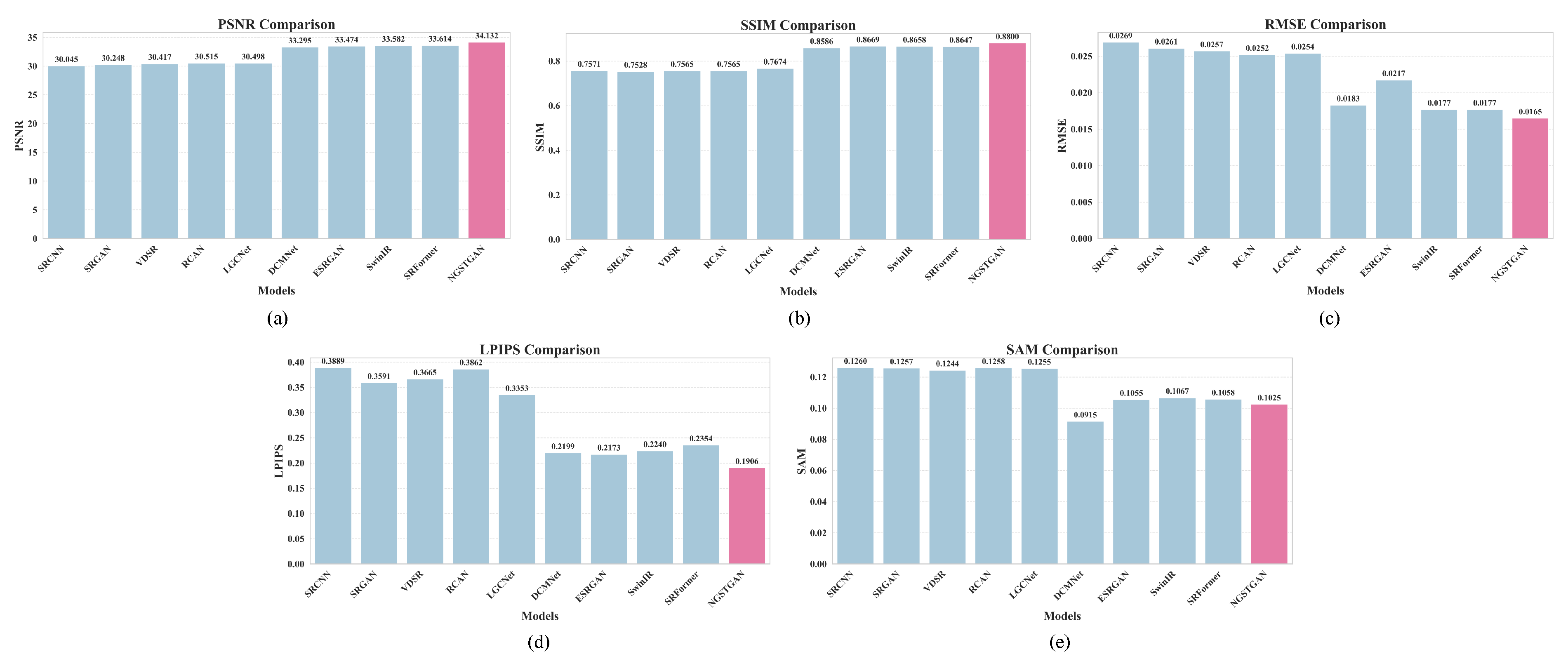
The baseline SwinIR model achieves a PSNR of 33.5820 dB and an SSIM of 0.8658, with corresponding RMSE, LPIPS, and SAM values of 0.0177, 0.2240, and 0.1067, respectively. It contains 5.05 M parameters and requires 32.35 G MACs. After integrating the NGWP module, consistent performance improvements are observed: PSNR increases to 33.6133 dB (+0.0313 dB); SSIM rises to 0.8673; and RMSE and LPIPS decrease to 0.0176 and 0.2224, respectively. These gains are accompanied by notable reductions in model size (3.77 M) and computational cost (20.43 G), underscoring NGWP’s ability to enhance performance while significantly improving efficiency. The inclusion of the ISFE module further boosts performance, raising PSNR to 34.0062 dB and SSIM to 0.8765, with RMSE and LPIPS dropping to 0.0168 and 0.1998, respectively. Crucially, these enhancements are achieved without increasing the parameter count or computational overhead, demonstrating the module’s effectiveness in improving reconstruction quality in a resource-efficient manner. When the discriminator is introduced alongside NGWP and ISFE, the model achieves its best performance: PSNR reaches 34.1317 dB, SSIM improves to 0.8800, RMSE and LPIPS are reduced to 0.0165 and 0.1906, and SAM declines to 0.1025. Compared to the baseline, this corresponds to gains of +0.5497 dB in PSNR and +0.0142 in SSIM and reductions of 0.0012, 0.0334, and 0.0042 in RMSE, LPIPS, and SAM, respectively—highlighting the synergistic effect of the proposed components. In conclusion, the NGWP module substantially improves feature interaction while achieving efficient model compression. When integrated with the ISFE module and the multi-attention discriminator, the overall NGSTGAN framework delivers notable improvements in both reconstruction accuracy and perceptual quality, validating the effectiveness and necessity of these components.

5.3. Advantages of Multi-Attention U-Net Discriminator

In GANs, a proficient discriminator is capable of more accurately distinguishing between generated images and real images, thereby prompting the generator to produce more realistic and high-quality SR images, particularly in the context of remotely sensed imagery, which can enhance detail fidelity and perceptual quality. The multi-attention U-Net discriminator proposed in this paper is adept at capturing the multi-scale features of RSIs, thereby guiding the generator to produce richer and more realistic RSIs. Additionally, the discriminator learns the representation of image edges and enhances its attention to critical details. To validate the effectiveness of the multi-attention u-net discriminator proposed in this paper, a series of experiments were conducted, including comparison and ablation studies. These experiments compared the performance of the proposed discriminator against several other discriminators, including no discriminator, the VGG discriminator [31], ViT discriminator [39], U-Net discriminator [32], and attention U-Net discriminator [38]. The results are summarized in

Table 6. Discriminator ablation experiments. Average quality evaluation of different discriminators on the test dataset. The top-performing results are marked in red, while the second-best are marked in blue. In the table, ↑ indicates that higher values are better, while ↓ means lower values are better.

Discriminator	PSNR ↑	SSIM ↑	RMSE ↓	LPIPS ↓	SAM ↓
No Discriminator	34.0062	0.8765	0.0168	0.1998	0.1034
VGG Discriminator	33.6057	0.8667	0.0177	0.2233	0.1062
ViT Discriminator	33.7029	0.8690	0.0175	0.2177	0.1057
U-Net Discriminator	34.0085	0.8769	0.0168	0.1972	0.1034
Attention U-Net Discriminator (No CSPA)	34.0651	0.8778	0.0167	0.1963	0.1030
Multi-Attention U-Net Discriminator (Ours)	34.1317	0.8800	0.0165	0.1906	0.1025

, which illustrates the impact of different discriminators on the model’s performance in the RSISR task and analyzes the performance differences. Without a discriminator, the model achieves baseline performance, with a PSNR of 34.0062 dB and an SSIM of 0.8765. The addition of a VGG discriminator results in decreases in PSNR of 0.4005 dB and SSIM of 0.0098, likely due to its limited feature extraction ability, failing to fully capture the detailed features of the inputs. The ViT discriminator shows a slight improvement in the model, with a decrease in PSNR of only 0.3033 dB compared to the baseline, but its SSIM still declines by 0.0075, and the model fails to outperform the baseline, possibly due to its reliance on the training data. The U-Net discriminator performs similarly to the no-discriminator scenario, with an increase in PSNR of 0.0023 dB and a slight increase in SSIM of 0.0004, indicating its robustness in extracting detailed features. The attention U-Net discriminator further optimizes the performance, with increases in PSNR of 0.0535 dB and SSIM of 0.0535 compared to the no-discriminator scenario. PSNR improves by 0.0589 dB and SSIM by 0.0013 compared to the no-discriminator scenario, thanks to its attention mechanism that can focus on key feature regions more effectively. Our proposed multi-attention U-Net discriminator performs the best, with improvements in PSNR of 0.1255 dB and SSIM of 0.0035 compared to the baseline and reductions in LPIPS and SAM of 0.0092 and 0.0009, respectively. These experimental results demonstrate that the multi-attention mechanism is capable of comprehensively capturing features, significantly improving generation quality and reconstruction accuracy while effectively suppressing reconstruction errors. Figure 16 illustrates the reconstruction effect of the network under different discriminators, revealing that our proposed multi-attention U-Net discriminator exhibits the best reconstruction quality, capable of reconstructing rich texture and edge information.

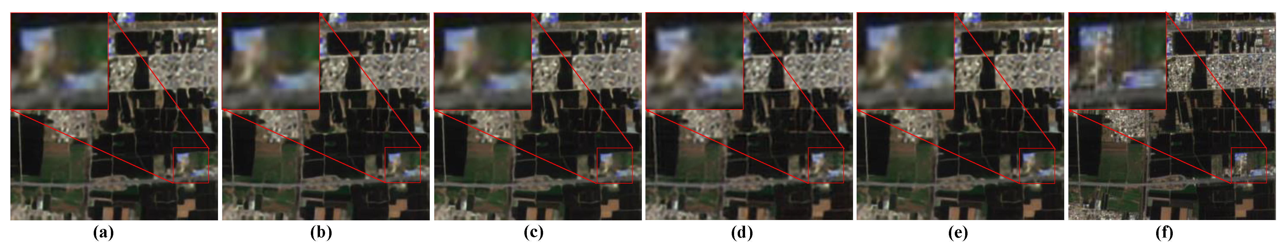
5.4. Discussion About Loss Function

The loss function plays a crucial role in guiding the optimization process of the model, directly influencing the quality and characteristics of the generated SR images. A well-chosen loss function not only aims to achieve pixel-level accuracy but also seeks to optimize visual perception, detail retention, and feature consistency. To thoroughly validate the effectiveness of the loss function proposed in this paper, a series of experiments were conducted, and the results are presented in

Table 7. Ablation experiments with loss functions. Evaluation of the average quality of different losses on the test dataset. The top-performing results are marked in red, while the second-best are marked in blue. In the table, ↑ indicates that higher values are better, while ↓ means lower values are better.

Loss Function Combination	PSNR ↑	SSIM ↑	RMSE ↓	LPIPS ↓	SAM ↓
${\mathcal{L}}_{\mathrm{pixel}}$	34.1011	0.8779	0.0164	0.1747	0.1028
${\mathcal{L}}_{\mathrm{pixel}}+{\mathcal{L}}_{\mathrm{VGG}}$	34.0062	0.8765	0.0168	0.1998	0.1034
${\mathcal{L}}_{\mathrm{pixel}}+{\mathcal{L}}_{\mathrm{RaGAN}}$	34.2499	0.8836	0.0167	0.1841	0.1027
${\mathcal{L}}_{\mathrm{VGG}}+{\mathcal{L}}_{\mathrm{RaGAN}}$	33.2955	0.8562	0.0186	0.2565	0.1068
${\mathcal{L}}_{\mathrm{pixel}}+{\mathcal{L}}_{\mathrm{VGG}}+{\mathcal{L}}_{\mathrm{RaGAN}}$ (Ours)	34.1317	0.8800	0.0165	0.1906	0.1025

. The table illustrates the impact of different loss function combinations on the SR images. In terms of various metrics, when ${\mathcal{L}}_{\mathrm{pixel}}$ is used alone, the SR image achieves the best PSNR (34.1011 dB), indicating a higher reconstruction quality, with the lowest RMSE (0.0164) and LPIPS (0.1747) suggesting that the pixel loss effectively recovers image details. However, despite the high PSNR, the optimization in this case lacks in visual quality. As shown in Figure 17, the image optimized with pixel loss is still rough in details and lacks realism. When ${\mathcal{L}}_{\mathrm{VGG}}$ is incorporated, the SSIM and other metrics related to visual quality (e.g., LPIPS and SAM) improve, enhancing the image’s structure and details, albeit with a slight decrease in PSNR (34.0062 dB). The goal of perceptual loss optimization is to reduce the perceived distance of the image, making the generated image closer to the real image in terms of data distribution. Although the PSNR decreases, the visual effect is more natural. The introduction of ${\mathcal{L}}_{\mathrm{RaGAN}}$ further improves PSNR and SSIM (34.2499 dB and 0.8836, respectively), with a slight increase in RMSE but reductions in LPIPS and SAM, indicating that the generated hyper-segmented images are more natural in perception and closer to the real images. Overall, the combination of perceptual loss and adversarial loss effectively enhances the visual quality, even if the PSNR index is slightly lower, making the images closer to the characteristics of real images. To mitigate the artifact issue caused by perceptual loss, the weight of perceptual loss was appropriately reduced in this study. Figure 17 presents a visual comparison of RSIs reconstructed by the network under different loss function optimizations.

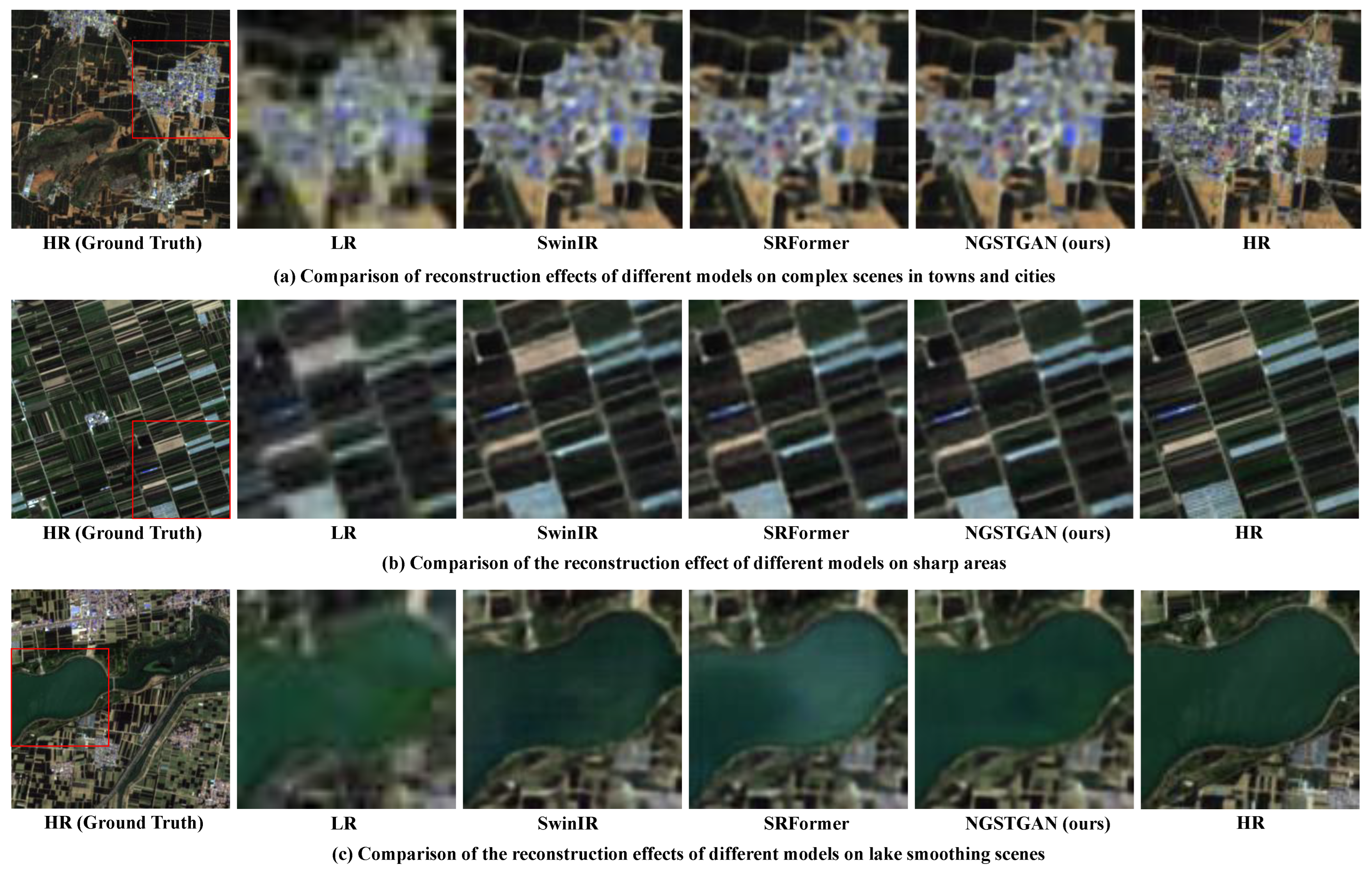
5.5. SR Results in Different Scenarios

RSIs encompass a variety of complex features, and there are significant differences in the reconstruction effects across different scenes. For this reason, we selected several typical scenes and analyzed their reconstruction effects in depth, comparing SwinIR, SRFormer, and the NGSTGAN model proposed in this paper.

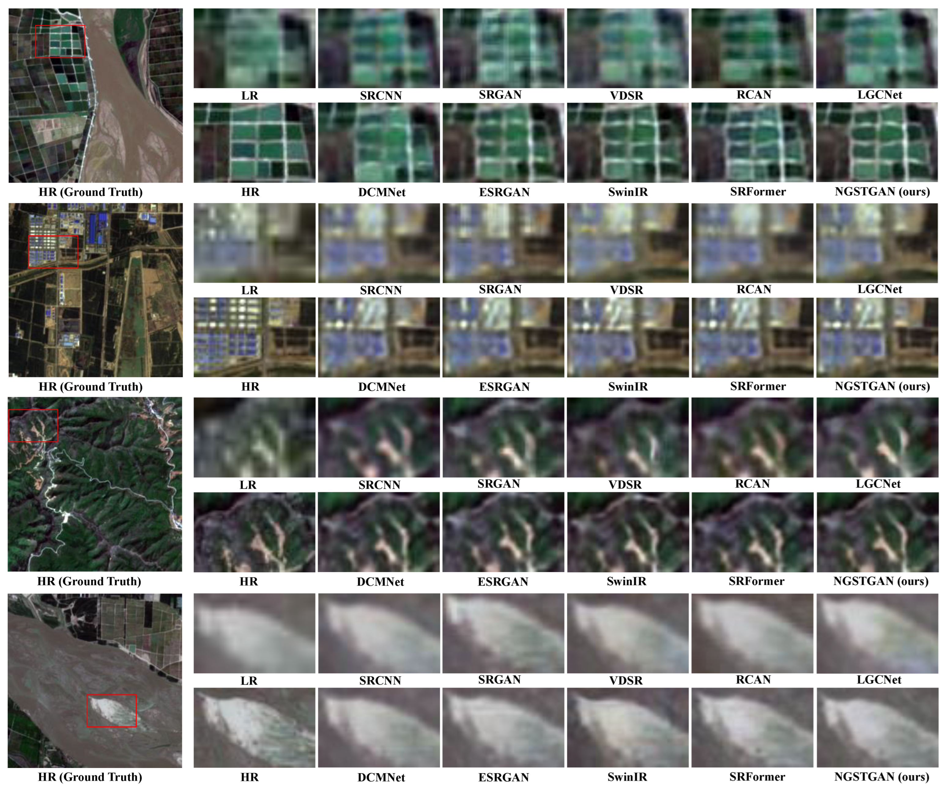
Figure 18a illustrates the reconstruction effects of different models in a complex town scene. Compared with other scenes, the features of the town scene are extremely complex and difficult to reconstruct, especially in the high-resolution (HR) image, where the edge features are also difficult to recognize, showing fuzzy highlighted areas. From the figure, we can see that, compared with SwinIR and SRFormer, the NGSTGAN model is more realistic in the reconstruction effect, successfully reconstructing spectral features, and the color performance is closer to the HR image. However, due to the high difficulty of reconstructing the urban construction scene, although the effect of NGSTGAN is improved, the overall reconstruction effect still has a certain gap compared with HR images.

Figure 18b shows the reconstruction effects of different models in a sharp-edge scene, which is a small piece of farmland. Although SwinIR and SRFormer partially recover the clarity of the image during the reconstruction process, there are still the problems of detail loss and blurring of the edges in the sharp areas. In contrast, the NGSTGAN model is outstanding in recovering the details and sharp edges of the image, effectively reducing the blurring phenomenon in the reconstruction and maintaining more original details, especially in the texture and edge parts of the image.

Figure 18c compares the reconstruction effects of several SR reconstruction models in a lake smoothing scene. The SwinIR and SRFormer models improve the image quality to some extent, partially restoring the smooth boundaries of the lake and the surrounding details. However, these two models are still deficient in the natural transition of lake texture and edge clarity. In contrast, the NGSTGAN model performs much better, not only significantly enhancing the smoothness of the lake region but also being able to preserve the details of the edge transition more finely. The color of the reconstruction result is closest to the HR image, and the overall reconstruction effect is closer to the real scene.

5.6. Analysis of Line Distortion in GAN-Based RSISR Results

GAN-based SR methods, including SRGAN and ESRGAN, often produce slight geometric distortions such as warping or bending of originally straight lines in man-made structures like roads and buildings. These distortions affect the geometric fidelity, which is crucial in remote sensing applications. Our proposed NGSTGAN achieves significant improvements in visual quality and detail reconstruction compared to SRGAN and ESRGAN. However, slight line distortions remain a challenge. To reduce this, we use a hybrid loss combining pixel-wise, perceptual, and adversarial losses, along with architectural enhancements like the ISFE module and an N-Gram-based S-WSA mechanism. Despite these advances, preserving strict geometric consistency requires further work. Future research will explore geometry-aware constraints to explicitly address line distortions and improve spatial accuracy in RSISR.

5.7. Complexity and Inference Time Comparison

Table 8. Comparative analysis of model complexity and IT (for the processing of 100 images). The top-performing results are marked in red, while the second-best are marked in blue. In the table, ↑ indicates that higher values are better, while ↓ means lower values are better.

Method	Parameters (M) ↓	MACs (G) ↓	IT (s) ↓
LGCNet	0.75	44.28	0.63
DCMNet	2.26	14.47	0.37
ESRGAN	9.79	59.93	0.98
SwinIR	5.05	32.35	0.74
SRFormer	3.04	19.35	0.46
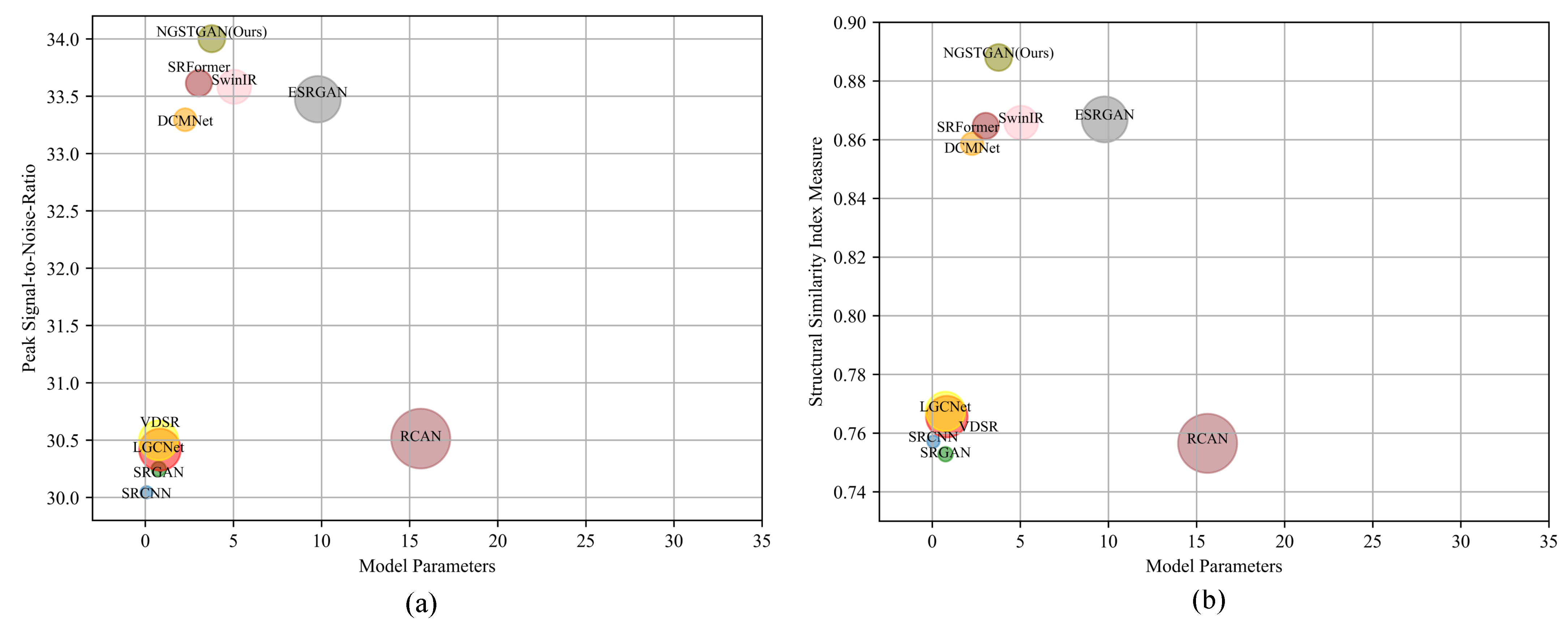
NGSTGAN	3.77	20.43	0.47

presents a comparative analysis of several representative models based on three key indicators: the number of parameters, MACs, and inference time (IT). These metrics collectively assess model efficiency and deployment cost from multiple perspectives. The number of parameters indicates the memory footprint, MACs reflect the theoretical computational complexity, and inference time measures the actual runtime performance on hardware platforms—serving as a crucial criterion for evaluating model compactness and real-time applicability. As shown in the table, LGCNet achieves the lowest parameter count, at only 0.75 M, reflecting an extremely compact network design. DCMNet excels in both MACs and inference speed, achieving the lowest values of 14.47 G and 0.37 s, respectively, for the processing of 100 images, thereby demonstrating a strong balance between speed and efficiency. SRFormer follows closely in terms of both computational cost and runtime, exhibiting a well-optimized trade-off. In comparison, the proposed NGSTGAN does not outperform all other models in any single metric but shows competitive performance across all three dimensions. It features a moderate parameter count of 3.77 M and 20.43 G MACs while achieving an inference time of 0.47 s for 100 images—comparable to SRFormer and significantly faster than larger models such as SwinIR and ESRGAN. These results indicate that NGSTGAN achieves an effective balance between reconstruction quality and computational efficiency, making it well-suited for real-world deployment. Overall, the comparative results not only validate the rationality of NGSTGAN’s architectural design but also highlight its potential for practical applications and scalable deployment scenarios.

5.8. Potential Applications of NGSTGAN

Although NGSTGAN is primarily designed for multispectral image super-resolution, its architectural components offer promising adaptability to other remote sensing tasks, such as pansharpening and pan-denoising. For pansharpening, methods like GPPNN [76] utilize gradient priors and deep fusion strategies to integrate spatial details from panchromatic images into multispectral data. NGSTGAN’s generator, built upon hierarchical Swin Transformer blocks enhanced with N-Gram contextual modeling, is well-suited to capture both fine-grained spatial structures and rich spectral information. With appropriate modifications—such as incorporating a high-resolution panchromatic branch and a suitable fusion module—NGSTGAN could be extended to achieve effective pan-guided fusion, preserving spectral integrity while enhancing spatial resolution. In the context of pan-denoising, as addressed by methods like PWRCTV [77], the objective is to suppress noise in hyperspectral or multispectral images using auxiliary panchromatic guidance. NGSTGAN’s multi-attention design and U-Net-based discriminator naturally facilitate the extraction of salient features while mitigating noise. With the integration of denoising-specific loss functions and training schemes, the model has the potential to be adapted for robust guided denoising tasks. These potential extensions highlight the versatility of the NGSTGAN framework and its relevance beyond its original application, providing a valuable foundation for future research in multimodal remote sensing image enhancement.

5.9. Limitations and Future Perspectives

The primary objective of this study is to investigate the potential of employing remote sensing image SR techniques to generate high-quality, multi-purpose data. Specifically, we aim to enhance the spatial resolution of Landsat-8 satellite imagery from 30 m to 10 m in the R, G, B, and NIR bands. In multispectral image SR tasks, effectively constraining the change of spectral information during the SR process is a critical challenge. However, this study did not incorporate an explicit spectral constraint mechanism; instead, it captured spectral features through implicit adaptive learning with the multiple-attention mechanism of NGSTGAN. Despite this, the results indicate that there is still a certain degree of spectral difference between the generated SR image and the real high-resolution image and a certain degree of color difference between the super-resolved image and the HR image. To further optimize the reconstruction accuracy of spectral information, we plan to introduce a joint spatial–spectral constraint loss function that explicitly corrects the spectral information of the low-resolution images, achieving joint SR in both spatial and spectral dimensions. Additionally, Landsat-8 satellite images cover a wide range of areas and contain a vast amount of data, making it challenging for current hardware resources to meet the demand for large-scale training. In the future, we aim to conduct SR processing for regions of specific research value and construct a high-resolution image dataset. Based on this dataset, we will further explore its potential in various remote sensing applications, such as land use classification, target detection, and crop extraction, to achieve higher precision application results. Furthermore, we plan to select specific areas for comprehensive SR of Landsat series images to construct a HR image dataset with a long time series. This dataset will provide high-quality basic data for further research and applications in the field of remote sensing, laying a solid foundation for the realization of high-precision analysis across multi-temporal and spatial scales.

6. Conclusions

In this study, we proposed an innovative RSISR method, NGSTGAN, to address the challenges of multi-scale feature extraction, limited WSA receptive fields, and high computational complexity faced by current RSISR methods. The method consists of two main parts: the generator, which is the N-Gram Swin Transformer, and the discriminator, which is the multi-attention U-Net. In the generator, we propose the ISFE module to substantially improve the network’s capacity for capturing complex textures and fine-grained details. Furthermore, to address the Swin Transformer’s limited receptive field, we incorporate the S-WSA mechanism and introduce the N-Gram concept to enhance contextual information exchange across adjacent windows. This design effectively boosts the accuracy of pixel-level reconstruction. The CRGC significantly reduces the number of parameters and complexity of the model. The discriminator multi-attention U-Net introduces channel, spatial, and pixel attention mechanisms, which can fully extract and discriminate the performance of RSIs in multi-scale feature recovery, effectively improving the attention and discrimination of key features. In addition, we constructed a four-band real-world multispectral remote sensing image SR dataset consisting of L8 and S2 images, which fills the gap in existing multispectral remote sensing image datasets. Based on this dataset, we conducted a series of experiments, and the results show that the proposed method outperforms other methods in improving the resolution of multispectral remote sensing imagery and is able to reconstruct sharper images. This provides a high-quality database for remote sensing applications, which can meet the demand for high-spatial-resolution RSIs in various fields.

References

1. Amit, S.N.K.B.; Shiraishi, S.; Inoshita, T.; Aoki, Y. Analysis of satellite images for disaster detection. In Proceedings of the 2016 IEEE International Geoscience and Remote Sensing Symposium (IGARSS), Beijing, China, 10–15 July 2016; IEEE: New York, NY, USA, 2016; pp. 5189–5192. [Google Scholar]
2. Zhang, Y.; Yang, G.; Gao, A.; Lv, W.; Xie, R.; Huang, M.; Liu, S. An efficient change detection method for disaster-affected buildings based on a lightweight residual block in high-resolution remote sensing images. Int. J. Remote Sens. 2023, 44, 2959–2981. [Google Scholar] [CrossRef]
3. Seelan, S.K.; Laguette, S.; Casady, G.M.; Seielstad, G.A. Remote sensing applications for precision agriculture: A learning community approach. Remote Sens. Environ. 2003, 88, 157–169. [Google Scholar] [CrossRef]
4. Bharadiya, J.P.; Tzenios, N.T.; Reddy, M. Forecasting of crop yield using remote sensing data, agrarian factors and machine learning approaches. J. Eng. Res. Rep. 2023, 24, 29–44. [Google Scholar] [CrossRef]
5. Li, R.; Shen, Y. YOLOSR-IST: A deep learning method for small target detection in infrared remote sensing images based on super-resolution and YOLO. Signal Process. 2023, 208, 108962. [Google Scholar] [CrossRef]
6. Lv, Z.; Zhang, P.; Sun, W.; Benediktsson, J.A.; Li, J.; Wang, W. Novel adaptive region spectral–spatial features for land cover classification with high spatial resolution remotely sensed imagery. IEEE Trans. Geosci. Remote Sens. 2023, 61, 1–12. [Google Scholar] [CrossRef]
7. Li, R.; Zheng, S.; Duan, C.; Wang, L.; Zhang, C. Land cover classification from remote sensing images based on multi-scale fully convolutional network. Geo-Spat. Inf. Sci. 2022, 25, 278–294. [Google Scholar] [CrossRef]
8. Vivone, G.; Alparone, L.; Chanussot, J.; Dalla Mura, M.; Garzelli, A.; Licciardi, G.A.; Restaino, R.; Wald, L. A critical comparison among pansharpening algorithms. IEEE Trans. Geosci. Remote Sens. 2014, 53, 2565–2586. [Google Scholar] [CrossRef]
9. Khaledyan, D.; Amirany, A.; Jafari, K.; Moaiyeri, M.H.; Khuzani, A.Z.; Mashhadi, N. Low-cost implementation of bilinear and bicubic image interpolation for real-time image super-resolution. In Proceedings of the 2020 IEEE Global Humanitarian Technology Conference (GHTC), Seattle, WA, USA, 29 October–1 November 2020; IEEE: New York, NY, USA, 2020; pp. 1–5. [Google Scholar]
10. Rasti, P.; Demirel, H.; Anbarjafari, G. Iterative back projection based image resolution enhancement. In Proceedings of the 2013 8th Iranian Conference on Machine Vision and Image Processing (MVIP), Zanjan, Iran, 10–12 September 2013; IEEE: New York, NY, USA, 2013; pp. 237–240. [Google Scholar]
11. Sun, J.; Xu, Z.; Shum, H.Y. Gradient profile prior and its applications in image super-resolution and enhancement. IEEE Trans. Image Process. 2010, 20, 1529–1542. [Google Scholar]
12. Yang, J.; Wright, J.; Huang, T.S.; Ma, Y. Image super-resolution via sparse representation. IEEE Trans. Image Process. 2010, 19, 2861–2873. [Google Scholar] [CrossRef]
13. Stark, H.; Oskoui, P. High-resolution image recovery from image-plane arrays, using convex projections. JOSA A 1989, 6, 1715–1726. [Google Scholar] [CrossRef]
14. LeCun, Y.; Bottou, L.; Bengio, Y.; Haffner, P. Gradient-based learning applied to document recognition. Proc. IEEE 1998, 86, 2278–2324. [Google Scholar] [CrossRef]
15. Dong, C.; Loy, C.C.; He, K.; Tang, X. Image super-resolution using deep convolutional networks. IEEE Trans. Pattern Anal. Mach. Intell. 2015, 38, 295–307. [Google Scholar] [CrossRef] [PubMed]
16. Dong, C.; Loy, C.C.; Tang, X. Accelerating the super-resolution convolutional neural network. In Proceedings of the Computer Vision–ECCV 2016: 14th European Conference, Amsterdam, The Netherlands, 11–14 October 2016; Proceedings, Part II 14. Springer: Berlin/Heidelberg, Germany, 2016; pp. 391–407. [Google Scholar]
17. He, K.; Zhang, X.; Ren, S.; Sun, J. Deep residual learning for image recognition. In Proceedings of the 2016 IEEE Conference on Computer Vision and Pattern Recognition (CVPR), Las Vegas, NV, USA, 27–30 June 2016; pp. 770–778. [Google Scholar]
18. Kim, J.; Lee, J.K.; Lee, K.M. Accurate image super-resolution using very deep convolutional networks. In Proceedings of the 2016 IEEE Conference on Computer Vision and Pattern Recognition (CVPR), Las Vegas, NV, USA, 27–30 June 2016; pp. 1646–1654. [Google Scholar]
19. Lim, B.; Son, S.; Kim, H.; Nah, S.; Mu Lee, K. Enhanced deep residual networks for single image super-resolution. In Proceedings of the 2017 IEEE Conference on Computer Vision and Pattern Recognition Workshops (CVPRW), Honolulu, HI, USA, 21–26 July 2017; pp. 136–144. [Google Scholar]
20. Tong, T.; Li, G.; Liu, X.; Gao, Q. Image super-resolution using dense skip connections. In Proceedings of the 2017 IEEE International Conference on Computer Vision (ICCV), Venice, Italy, 22–29 October 2017; pp. 4799–4807. [Google Scholar]
21. Zhang, Y.; Tian, Y.; Kong, Y.; Zhong, B.; Fu, Y. Residual dense network for image super-resolution. In Proceedings of the 2018 IEEE/CVF Conference on Computer Vision and Pattern Recognition, Salt Lake City, UT, USA, 18–23 June 2018; pp. 2472–2481. [Google Scholar]
22. Zhang, Y.; Li, K.; Li, K.; Wang, L.; Zhong, B.; Fu, Y. Image super-resolution using very deep residual channel attention networks. In Proceedings of the Computer Vision–ECCV 2018 15th European Conference, Munich, Germany, 8–14 September 2018; pp. 286–301. [Google Scholar]
23. Dai, T.; Cai, J.; Zhang, Y.; Xia, S.T.; Zhang, L. Second-order attention network for single image super-resolution. In Proceedings of the 2019 IEEE/CVF Conference on Computer Vision and Pattern Recognition (CVPR), Long Beach, CA, USA, 15–20 June 2019; pp. 11065–11074. [Google Scholar]
24. Shi, Z.; Chen, C.; Xiong, Z.; Liu, D.; Zha, Z.J.; Wu, F. Deep residual attention network for spectral image super-resolution. In Proceedings of the Computer Vision–ECCV 2018 15th European Conference, Munich, Germany, 8–14 September 2018. [Google Scholar]
25. Zhao, H.; Kong, X.; He, J.; Qiao, Y.; Dong, C. Efficient image super-resolution using pixel attention. In Proceedings of the Computer Vision–ECCV 2020 Workshops, Glasgow, UK, 23–28 August 2020; Proceedings, Part III 16. Springer: Berlin/Heidelberg, Germany, 2020; pp. 56–72. [Google Scholar]
26. Richards, J.A.; Richards, J.A. Remote Sensing Digital Image Analysis; Springer: Berlin/Heidelberg, Germany, 2022; Volume 5. [Google Scholar]
27. Lei, S.; Shi, Z.; Zou, Z. Super-resolution for remote sensing images via local–global combined network. IEEE Geosci. Remote Sens. Lett. 2017, 14, 1243–1247. [Google Scholar] [CrossRef]
28. Lei, S.; Shi, Z. Hybrid-scale self-similarity exploitation for remote sensing image super-resolution. IEEE Trans. Geosci. Remote Sens. 2021, 60, 1–10. [Google Scholar] [CrossRef]
29. Dong, X.; Sun, X.; Jia, X.; Xi, Z.; Gao, L.; Zhang, B. Remote sensing image super-resolution using novel dense-sampling networks. IEEE Trans. Geosci. Remote Sens. 2020, 59, 1618–1633. [Google Scholar] [CrossRef]
30. Chen, L.; Liu, H.; Yang, M.; Qian, Y.; Xiao, Z.; Zhong, X. Remote sensing image super-resolution via residual aggregation and split attentional fusion network. IEEE J. Sel. Top. Appl. Earth Obs. Remote Sens. 2021, 14, 9546–9556. [Google Scholar] [CrossRef]
31. Ledig, C.; Theis, L.; Huszár, F.; Caballero, J.; Cunningham, A.; Acosta, A.; Aitken, A.; Tejani, A.; Totz, J.; Wang, Z. Photo-realistic single image super-resolution using a generative adversarial network. In Proceedings of the 2017 IEEE Conference on Computer Vision and Pattern Recognition (CVPR), Honolulu, HI, USA, 21–26 July 2017; pp. 4681–4690. [Google Scholar]
32. Wang, X.; Yu, K.; Wu, S.; Gu, J.; Liu, Y.; Dong, C.; Qiao, Y.; Change Loy, C. Esrgan: Enhanced super-resolution generative adversarial networks. In Proceedings of the Computer Vision—ECCV 2018 15th European Conference, Munich, Germany, 8–14 September 2018. [Google Scholar]
33. Wang, X.; Xie, L.; Dong, C.; Shan, Y. Real-esrgan: Training real-world blind super-resolution with pure synthetic data. In Proceedings of the 2021 IEEE/CVF International Conference on Computer Vision Workshops (ICCVW), Montreal, BC, Canada, 11–17 October 2021; pp. 1905–1914. [Google Scholar]
34. Jiang, K.; Wang, Z.; Yi, P.; Wang, G.; Lu, T.; Jiang, J. Edge-enhanced GAN for remote sensing image superresolution. IEEE Trans. Geosci. Remote Sens. 2019, 57, 5799–5812. [Google Scholar] [CrossRef]
35. Jia, S.; Wang, Z.; Li, Q.; Jia, X.; Xu, M. Multiattention generative adversarial network for remote sensing image super-resolution. IEEE Trans. Geosci. Remote Sens. 2022, 60, 1–15. [Google Scholar] [CrossRef]
36. Dong, R.; Zhang, L.; Fu, H. RRSGAN: Reference-based super-resolution for remote sensing image. IEEE Trans. Geosci. Remote Sens. 2021, 60, 1–17. [Google Scholar] [CrossRef]
37. Lei, S.; Shi, Z.; Zou, Z. Coupled adversarial training for remote sensing image super-resolution. IEEE Trans. Geosci. Remote Sens. 2019, 58, 3633–3643. [Google Scholar] [CrossRef]
38. Wei, Z.; Huang, Y.; Chen, Y.; Zheng, C.; Gao, J. A-ESRGAN: Training real-world blind super-resolution with attention U-Net Discriminators. In Proceedings of the 20th Pacific Rim International Conference on Artificial Intelligence, Jakarta, Indonesia, 15–19 November 2023; Springer: Berlin/Heidelberg, Germany, 2023; pp. 16–27. [Google Scholar]
39. Wang, C.; Zhang, X.; Yang, W.; Wang, G.; Li, X.; Wang, J.; Lu, B. MSWAGAN: Multi-spectral remote sensing image super resolution based on multi-scale window attention transformer. IEEE Trans. Geosci. Remote Sens. 2024. [Google Scholar]
40. Vaswani, A. Attention is all you need. In Advances in Neural Information Processing Systems; The MIT Press: Cambridge, MA, USA, 2017. [Google Scholar]
41. Dosovitskiy, A. An image is worth 16x16 words: Transformers for image recognition at scale. arXiv 2020, arXiv:2010.11929. [Google Scholar]
42. Liu, Z.; Lin, Y.; Cao, Y.; Hu, H.; Wei, Y.; Zhang, Z.; Lin, S.; Guo, B. Swin transformer: Hierarchical vision transformer using shifted windows. In Proceedings of the 2021 IEEE/CVF International Conference on Computer Vision (ICCV), Montreal, QC, Canada, 10–17 October 2021; pp. 10012–10022. [Google Scholar]
43. Liang, J.; Cao, J.; Sun, G.; Zhang, K.; Van Gool, L.; Timofte, R. Swinir: Image restoration using swin transformer. In Proceedings of the 2021 IEEE/CVF International Conference on Computer Vision Workshops (ICCVW), Montreal, BC, Canada, 11–17 October 2021; pp. 1833–1844. [Google Scholar]
44. Zhou, Y.; Li, Z.; Guo, C.L.; Bai, S.; Cheng, M.M.; Hou, Q. Srformer: Permuted self-attention for single image super-resolution. In Proceedings of the 2023 IEEE/CVF International Conference on Computer Vision (ICCV), Paris, France, 1–6 October 2023; pp. 12780–12791. [Google Scholar]
45. Xiao, T.; Singh, M.; Mintun, E.; Darrell, T.; Dollár, P.; Girshick, R. Early convolutions help transformers see better. Adv. Neural Inf. Process. Syst. 2021, 34, 30392–30400. [Google Scholar]
46. Xiao, Y.; Yuan, Q.; Jiang, K.; He, J.; Lin, C.W.; Zhang, L. TTST: A top-k token selective transformer for remote sensing image super-resolution. IEEE Trans. Image Process. 2024, 33, 738–752. [Google Scholar] [CrossRef]
47. Zhang, K.; Li, L.; Jiao, L.; Liu, X.; Ma, W.; Liu, F.; Yang, S. CSCT: Channel-Spatial Coherent Transformer for Remote Sensing Image Super-Resolution. IEEE Trans. Geosci. Remote Sens. 2025, 63, 5611014. [Google Scholar] [CrossRef]
48. Tu, J.; Mei, G.; Ma, Z.; Piccialli, F. SWCGAN: Generative adversarial network combining swin transformer and CNN for remote sensing image super-resolution. IEEE J. Sel. Top. Appl. Earth Obs. Remote Sens. 2022, 15, 5662–5673. [Google Scholar] [CrossRef]
49. Majumder, P.; Mitra, M.; Chaudhuri, B. N-gram: A language independent approach to IR and NLP. In Proceedings of the International Conference on Universal Knowledge and Language, Goa, India, 25–29 November 2002; Volume 2. [Google Scholar]
50. Pagliardini, M.; Gupta, P.; Jaggi, M. Unsupervised learning of sentence embeddings using compositional n-gram features. arXiv 2017, arXiv:1703.02507. [Google Scholar]
51. Lopez-Gazpio, I.; Maritxalar, M.; Lapata, M.; Agirre, E. Word n-gram attention models for sentence similarity and inference. Expert Syst. Appl. 2019, 132, 1–11. [Google Scholar] [CrossRef]
52. Kulkami, P.; Stranieri, A.; Ugon, J. Texture image classification using pixel N-grams. In Proceedings of the 2016 IEEE International Conference on Signal and Image Processing (ICSIP), Beijing, China, 13–15 August 2016; IEEE: New York, NY, USA, 2016; pp. 137–141. [Google Scholar]
53. He, X.; Huang, T.; Bai, S.; Bai, X. View n-gram network for 3d object retrieval. In Proceedings of the 2019 IEEE/CVF International Conference on Computer Vision (ICCV), Seoul, Republic of Korea, 27 October 2019–2 November 2019; pp. 7515–7524. [Google Scholar]
54. Choi, H.; Lee, J.; Yang, J. N-gram in swin transformers for efficient lightweight image super-resolution. In Proceedings of the 2023 IEEE/CVF Conference on Computer Vision and Pattern Recognition (CVPR), Vancouver, BC, Canada, 17–24 June 2023; pp. 2071–2081. [Google Scholar]
55. Zhang, X.; Zhou, X.; Lin, M.; Sun, J. Shufflenet: An extremely efficient convolutional neural network for mobile devices. In Proceedings of the 2018 IEEE/CVF Conference on Computer Vision and Pattern Recognition, Salt Lake City, UT, USA, 18–23 June 2018; pp. 6848–6856. [Google Scholar]
56. Tan, M.; Le, Q. Efficientnet: Rethinking model scaling for convolutional neural networks. In Proceedings of the 36th International Conference on Machine Learning (ICML), Long Beach, CA, USA, 9–15 June 2019; pp. 6105–6114. [Google Scholar]
57. Zhou, Z.; Rahman Siddiquee, M.M.; Tajbakhsh, N.; Liang, J. Unet++: A nested u-net architecture for medical image segmentation. In Proceedings of the Deep Learning in Medical Image Analysis and Multimodal Learning for Clinical Decision Support: 4th International Workshop, DLMIA 2018, and 8th International Workshop, ML-CDS 2018, Granada, Spain, 20 September 2018; Proceedings 4. Springer: Berlin/Heidelberg, Germany, 2018; pp. 3–11. [Google Scholar]
58. Cohen, T.; Welling, M. Group equivariant convolutional networks. In Proceedings of the 33rd International Conference on Machine Learning (ICML 2016), New York, NY, USA, 19–24 June 2016; pp. 2990–2999. [Google Scholar]
59. Chen, Y.; Weng, Q.; Tang, L.; Zhang, X.; Bilal, M.; Li, Q. Thick clouds removing from multitemporal Landsat images using spatiotemporal neural networks. IEEE Trans. Geosci. Remote Sens. 2020, 60, 1–14. [Google Scholar] [CrossRef]
60. Gao, G.; Gu, Y. Multitemporal Landsat missing data recovery based on tempo-spectral angle model. IEEE Trans. Geosci. Remote Sens. 2017, 55, 3656–3668. [Google Scholar] [CrossRef]
61. Elsayed, G.; Ramachandran, P.; Shlens, J.; Kornblith, S. Revisiting spatial invariance with low-rank local connectivity. In Proceedings of the 37th International Conference on Machine Learning, Virtual Event, 13–18 July 2020; pp. 2868–2879. [Google Scholar]
62. Vaswani, A.; Ramachandran, P.; Srinivas, A.; Parmar, N.; Hechtman, B.; Shlens, J. Scaling local self-attention for parameter efficient visual backbones. In Proceedings of the 2021 IEEE/CVF Conference on Computer Vision and Pattern Recognition (CVPR), Nashville, TN, USA, 20–25 June 2021; pp. 12894–12904. [Google Scholar]
63. Simonyan, K.; Zisserman, A. Very deep convolutional networks for large-scale image recognition. arXiv 2014, arXiv:1409.1556. [Google Scholar]
64. Jolicoeur-Martineau, A. The relativistic discriminator: A key element missing from standard GAN. arXiv 2018, arXiv:1807.00734. [Google Scholar]
65. Hore, A.; Ziou, D. Image quality metrics: PSNR vs. SSIM. In Proceedings of the 2010 20th International Conference on Pattern Recognition, Istanbul, Turkey, 23–26 August 2010; IEEE: New York, NY, USA, 2010; pp. 2366–2369. [Google Scholar]
66. Wang, Z.; Bovik, A.C.; Sheikh, H.R.; Simoncelli, E.P. Image quality assessment: From error visibility to structural similarity. IEEE Trans. Image Process. 2004, 13, 600–612. [Google Scholar] [CrossRef] [PubMed]
67. Gore, A.; Kansal, H.; Gupta, S. Local standard deviation based image quality metrics for jpeg compressed images. TELKOMNIKA Indones. J. Electr. Eng. 2014, 12, 7280–7286. [Google Scholar] [CrossRef]
68. Kruse, F.A.; Lefkoff, A.; Boardman, y.J.; Heidebrecht, K.; Shapiro, A.; Barloon, P.; Goetz, A. The spectral image processing system (SIPS)—interactive visualization and analysis of imaging spectrometer data. Remote Sens. Environ. 1993, 44, 145–163. [Google Scholar] [CrossRef]
69. Zhang, R.; Isola, P.; Efros, A.A.; Shechtman, E.; Wang, O. The unreasonable effectiveness of deep features as a perceptual metric. In Proceedings of the 2018 IEEE/CVF Conference on Computer Vision and Pattern Recognition, Salt Lake City, UT, USA, 18–23 June 2018; pp. 586–595. [Google Scholar]
70. Sandler, M.; Howard, A.; Zhu, M.; Zhmoginov, A.; Chen, L.C. Mobilenetv2: Inverted residuals and linear bottlenecks. In Proceedings of the 2018 IEEE/CVF Conference on Computer Vision and Pattern Recognition, Salt Lake City, UT, USA, 18–23 June 2018; pp. 4510–4520. [Google Scholar]
71. Howard, A.G. Mobilenets: Efficient convolutional neural networks for mobile vision applications. arXiv 2017, arXiv:1704.04861. [Google Scholar]
72. Rogozhnikov, A. Einops: Clear and reliable tensor manipulations with einstein-like notation. In Proceedings of the International Conference on Learning Representations, Vienna, Austria, 4 May 2021. [Google Scholar]
73. Paszke, A.; Gross, S.; Massa, F.; Lerer, A.; Bradbury, J.; Chanan, G.; Killeen, T.; Lin, Z.; Gimelshein, N.; Antiga, L. Pytorch: An imperative style, high-performance deep learning library. In Advances in Neural Information Processing Systems; The MIT Press: Cambridge, MA, USA, 2019; Volume 32. [Google Scholar]
74. Loshchilov, I. Decoupled weight decay regularization. arXiv 2017, arXiv:1711.05101. [Google Scholar]
75. Zhang, C.; Zhang, M.; Li, Y.; Gao, X.; Qiu, S. Difference Curvature Multidimensional Network for Hyperspectral Image Super-Resolution. Remote Sens. 2021, 13, 3455. [Google Scholar] [CrossRef]
76. Xu, S.; Zhang, J.; Zhao, Z.; Sun, K.; Liu, J.; Zhang, C. Deep gradient projection networks for pan-sharpening. In Proceedings of the 2021 IEEE/CVF Conference on Computer Vision and Pattern Recognition (CVPR), Nashville, TN, USA, 20–25 June 2021; pp. 1366–1375. [Google Scholar]
77. Xu, S.; Ke, Q.; Peng, J.; Cao, X.; Zhao, Z. Pan-Denoising: Guided Hyperspectral Image Denoising via Weighted Represent Coefficient Total Variation. IEEE Trans. Geosci. Remote Sens. 2024, 62, 5528714. [Google Scholar] [CrossRef]
Figure 1. N-Grams in text. The underlined words represent the target words, while the non-underlined words serve as the neighbors of these target words.
Remotesensing 17 02079 g001
Figure 2. N-Grams in an image. Each local window is considered a uni-Gram, while the lower-right (or upper-left) local windows are treated as forward (or backward) N-Gram neighbors.
Remotesensing 17 02079 g002
Figure 3. Overall architecture of the proposed NGSTGAN. The framework consists of (a) a generator based on the N-Gram Swin Transformer, comprising a shallow feature extraction module, a deep feature extraction module with N-Gram Residual Swin Transformer Blocks (NGRSTBs), and an HR image reconstruction module, and (b) a multi-attention U-Net discriminator incorporating attention blocks, concatenate blocks, and channel–spatial–pixel attention modules.
Remotesensing 17 02079 g003
Figure 4. Detailed architecture of the improved shallow feature extraction (ISFE) module. The design integrates five parallel convolutional kernel branches with specialized transformations—including center difference, angle-directional modulation, horizontal difference, and vertical difference—to enhance multi-scale and directional feature extraction, followed by unified kernel-weight fusion for shallow representation learning.
Remotesensing 17 02079 g004
Figure 5. The process diagram of N-Gram window partition. k, s, p, g r o u p , and W are the convolutional kernel size, step size, padding, number of groups, and size of the local window, respectively. Channel-reducing group convolution, sequential reflection window padding, and sliding window self-attention work together to introduce the N-Gram idea while reducing the number of parameters and MACs.
Remotesensing 17 02079 g005
Figure 6. Sequential reflection window padding and sliding window self-attention in the N-Gram window partition module, where the value of N is set to 2. When the window is slid in uni-Gram embedding, it is pooled by WSA and averaged to obtain forward and backward N-Gram features.
Remotesensing 17 02079 g006
Figure 7. Detailed architecture of key attention components in the proposed multi-attention U-Net discriminator. (a) The attention block integrates encoder and bridge features through a spatial attention mechanism to enhance salient region focus. (b) The channel, spatial, and pixel attention module combines three attention sub-modules to sequentially refine features in the encoder by emphasizing informative channels, highlighting spatially relevant regions, and enhancing pixel-level details.
Remotesensing 17 02079 g007
Figure 8. In this study, we use paired image patches from various scenarios to train the SR model. The 10 m HR S2 images are placed in the first row, while the 30 m LR L8 images are in the second row.
Remotesensing 17 02079 g008
Figure 9. Comparison plot of PSNR and SSIM variation with training rounds for different models on validation data.
Remotesensing 17 02079 g009
Figure 10. The number of parameters and average performance on the test dataset, with MACs represented by scatter magnitude.
Remotesensing 17 02079 g010
Figure 11. Performance comparison of NGSTGAN with leading super-resolution models across PSNR (a), SSIM (b), RMSE (c), LPIPS (d), and SAM (e).
Remotesensing 17 02079 g011
Figure 12. Global reconstruction effect of different models (I). The red box highlights the emphasized region.
Remotesensing 17 02079 g012
Figure 13. Global reconstruction effects of different models (II). The red box highlights the emphasized region.
Remotesensing 17 02079 g013
Figure 14. Localized reconstruction renderings of different models, including farmland, towns, mountains, and rivers. The red boxes indicate the regions of interest that are enlarged for visual comparison.
Remotesensing 17 02079 g014
Figure 15. The reconstruction effect of our method on each band of the image.
Remotesensing 17 02079 g015
Figure 16. Visual comparison of NGSTGAN-reconstructedSR images with different discriminators. (a) LR image. (b) No discriminator. (c) VGG discriminator. (d) ViT discriminator. (e) U-Net discriminator. (f) Attention U-Net discriminator. (g) Multi-attention U-Net discriminator (Ours). (h) HR image.
Remotesensing 17 02079 g016
Figure 17. Visual comparison of network-reconstructed SR images under different loss function optimizations. (a) L pixel . (b) L pixel + L VGG . (c) L pixel + L RaGAN . (d) L VGG + L RaGAN . (e) L pixel + L VGG + L RaGAN (Ours). (f) HR image.
Remotesensing 17 02079 g017
Figure 18. Comparison of reconstruction effects of different models on different scenes. The red boxes indicate the regions of interest that are enlarged for visual comparison.
Remotesensing 17 02079 g018