Abstract
Estimating wheat traits based on spectral reflectance measurements and machine learning remains challenging due to the large datasets required for model training and testing. To overcome this limitation, a simulated dataset was generated using the radiative transfer model (RTM) PROSAIL and inverted based on an artificial neural network (ANN). Field experiments were conducted in Eastern Austria to measure spectral reflectance and destructively sample plants to measure the wheat traits plant area index (PAI), nitrogen yield (NY), canopy water content (CWC), and above-ground dry matter (AGDM). Four ANN-based RTM inversion models were setup, which varied in their spectral resolution, hyperspectral or multispectral, and the inclusion or exclusion of background soil spectra correction. The models were also compared to a simple vegetation index approach using Normalized Difference Vegetation Index (NDVI) and Normalized Difference Red-Edge (NDRE). The RTM inversion model with hyperspectral input data and background soil spectra correction was the best among all tested models for estimating wheat traits during the vegetative developmental stages (PAI: R2 = 0.930, RRMSE = 17.9%; NY: R2 = 0.908, RRMSE = 14.4%; CWC: R2 = 0.967, RRMSE = 17.0%) as well as throughout the whole growing season (PAI: R2 = 0.845, RRMSE = 27.7%; CWC: R2 = 0.884, RRMSE = 20.0%; AGDM: R2 = 0.960, RRMSE = 13.7%). Many models presented in this study provided suitable estimations of the relevant wheat traits PAI, NY, CWC, and AGDM for application in agronomy, breeding, and crop sciences in general.
1. Introduction
Traditionally, measurements of wheat traits (Triticum aestivum L.) are often destructive and time-consuming. An alternative is the estimation of traits using remote sensing, i.e., the measurement of the reflected or emitted electromagnetic radiation of objects, which is non-destructive, faster, and less labor-intensive than destructive sampling [1,2,3].
A common approach to estimate plant traits based on remote sensing is the application of vegetation indices, which are calculations based on spectral reflectance data of vegetation. This technique is simple and generally provides good results [4,5,6,7,8]. The calculation of vegetation indices, however, is usually based on only two or three spectral bands, i.e., regions of the electromagnetic spectrum defined by their wavelength in nm. Therefore, not all collected spectral data are used [9,10].
An alternative approach is the use of machine learning algorithms [11,12], i.e., the development of model algorithms including training and testing. This technique can utilize all available spectral data, but usually requires large datasets for model training [13]. To overcome this limitation of machine learning, Reinosch et al. [14] proposed to train models with empirically collected data augmented by simulated data, which are generated with existing mechanistic models. In the context of estimating plant traits based on spectral data, radiative transfer models (RTMs) can be utilized as the mechanistic models, as suggested by Reinosch et al. [14].
In general, RTMs simulate the spectral reflectance of leaves and canopies (RTM output), which requires information on various leaf and canopy traits (RTM input). To estimate plant traits based on spectral data, however, the inputs and outputs of RTMs need to be inverted [9,15,16]. This can be achieved by, e.g., look-up tables [17,18] or machine learning algorithms [19,20,21]. With this approach, all available spectral data can be used for estimating plant traits [16], similar to classic machine learning. Additionally, the limitation by scarce empirical data in traditional machine learning is offset by the inclusion of simulated data based on mechanistic models, e.g., inverted RTMs [14]. Furthermore, the use of mechanistic models allows for a wider generalization of the results and, thus, reduces the need for recalibration for different cultivars or environments [16].
The RTM inversion approach results in complex models that require specific training for the individual spectral resolution of a given sensor, e.g., the position, width, and number of spectral bands [20]. The simulation of canopy reflectance spectra is also substantially affected by the soil background reflectance [22]. This effect is especially prevalent when the canopy cover is low, e.g., at early and late developmental stages [16]. Furthermore, the soil background reflectance varies greatly across and within seasons and locations [23,24]. Therefore, wheat traits were estimated in this study using the spectral reflectance of both canopies and underlying soil combined to adequately account for soil background effects.
In this study, the traits plant area index (PAI, m2 m−2), nitrogen yield (NY, g m−2), canopy water content (CWC, g m−2), and above-ground dry matter (AGDM, g m−2) were estimated in wheat using an artificial neural network (ANN)-based inversion of the RTM PROSAIL [25]. The models were further trained and tested with data on destructively sampled plants as well as spectral reflectance, which were collected from wheat field experiments in Eastern Austria for two seasons. Different aspects of these field experimental data were investigated in previous studies. Koppensteiner et al. [26] presented a detailed yield and yield component analysis. Bernas et al. [27] conducted a life cycle assessment to find the environmentally optimal N fertilization rate in wheat. Furthermore, Moitzi et al. [28] studied the effects of sowing time and nitrogen fertilizer rate on energy efficiency.
The objectives of this study were to conduct (1) the ANN-based RTM inversion and (2) estimate wheat traits based on the RTM inversion models to present the feasibility of this approach and provide a guide for setting up similar models also for different crops or other spectral sensors. Furthermore, this study evaluated certain aspects of model performances: the differences between varying spectral resolutions, i.e., hyperspectral and multispectral, the effects of including or excluding the background soil spectra correction, as well as the comparison of performances between complex RTM inversion models and simple vegetation index models.
2. Materials and Methods
2.1. Overview
In this section, an overview of the main steps conducted in this study is presented. In the following sections, the individual steps are presented in detail.
Firstly, field experimental data (Section 2.2) were collected in two seasons, which consists of reflectance measurements and destructive plant samples. Secondly, the RTM PROSAIL (Section 2.3) was used to create a simulated dataset (Section 2.4). Thirdly, an ANN (Section 2.5) was trained on the simulated dataset to achieve the RTM inversion. The model input was reflectance data. The model output consisted of the leaf and canopy traits of the RTM PROSAIL. Fourthly, the experimentally collected reflectance data were processed (Section 2.5) and then used by the RTM inversion model to calculate wheat trait estimates. Furthermore, the same experimental reflectance data were applied to calculate the vegetation indices NDVI and NDRE.
Finally, simple regression models were created for model evaluation (Section 2.6). The model inputs were the wheat trait estimates by the RTM inversion models or vegetation indices. The model outputs were the target wheat traits PAI, NY, CWC, and AGDM, which were measured destructively in the field experiments. The regression models were trained on one season of the field experimental data and tested on the field experimental data of the other season.
2.2. The Field Experimental Dataset
Field experiments were performed in the growing seasons of 2019/20 and 2020/21 at the Experimental Farm Groß-Enzersdorf of the University of Natural Resources and Life Sciences, Vienna (48° 11′N, 16° 33′E) in Eastern Austria. The soil at the experimental site was classified as chernozem of alluvial origin, which is rich in calcareous sediments and has a pHCaCl2 of 7.6 and 2.3% soil organic carbon [29].
The mean annual temperature and the mean annual precipitation sum from 1980 to 2018 were 10.9 °C and 546 mm, respectively. The two experimental seasons showed highly varying environmental conditions with low amounts of precipitation in March and April for both seasons and in June 2021, high temperature in March 2020, as well as low temperature in April and May 2021. Further detailed information on the temperature and precipitation during the growing periods of the conducted field experiments can be obtained from Koppensteiner et al. [26].
In both experimental seasons, the preceding crop was winter barley. A tine cultivator was used for primary soil tillage to 20 cm depth. Seedbed preparation was conducted using a power harrow at a shallow tilling depth.
The field experiments were established in a split-plot design. The experimental factors were the sowing time with two factor levels, autumn- and spring-sowing, as well as nitrogen fertilization consisting of five levels of 0, 5, 10, 15, and 20 g N m−2. The main plot factor sowing time was set up in complete blocks, while the sub-plot factor nitrogen fertilization was randomized among sub-plots within the main plots. The field experiments were conducted in three replications.
The facultative wheat cultivar Lennox was sown with 300 germinable seeds m−2 on 17 October 2019 and 10 March 2020 as well as 27 October 2020 and 8 March 2021 using an Oyjard plot drill seeder at 4 cm depth. Plot dimensions were 12 × 3 m (36 m2). Row spacing was 12.5 cm. Nitrogen fertilizer was applied as stabilized urea (46% nitrogen, ALZON 46®, SKW Piesteritz, Lutherstadt Wittenberg, Germany) on 10 March 2020 and 10 March 2021. Weeds, pests, and diseases were controlled according to good agricultural practice. Details on plant protection measures were presented in Koppensteiner et al. [26].
In both seasons, data on crop development, plant area index (PAI, m2 m−2), above-ground dry matter (AGDM, g m−2), nitrogen yield (NY, g m−2), and canopy water content (CWC, g m−2) were collected at approximately 14-day intervals from March until harvest in July.
Crop development was recorded according to the BBCH scale [30,31]. Plants were sampled by manually cutting 0.6 m2 per plot at soil surface during the growing season except for the final harvest date, when 1.2 m2 per plot were cut. The plant area index (m2 m−2) of fresh plant material was measured using the LI-3100C Area Meter (LI-COR Inc., Lincoln, OR, USA).
Plant samples were weighed fresh and after drying at 105 °C for 24 h (UNE 600, Memmert GmbH & Co. KG, Schwabach, Germany). Weight before drying corresponds to above-ground fresh matter (AGFM, g m−2). Weight after drying is referred to as AGDM gravimetric canopy water content (CWC, g m−2) and is calculated as:
Plant material was milled to pass through a 1 mm sieve and dried at 105 °C for 24 h. Milled plant samples were analyzed for nitrogen concentration by the Dumas combustion method [32] using an element analyzer (vario MAX cube CNS, Elementar Analysesysteme, Langenselbold, Germany). The resulting nitrogen concentration values (NC, %) were multiplied by AGDM to calculate the nitrogen yield (NY, g m−2):
Autumn-sown wheat was harvested on 6 July 2020 and 13 July 2021. Spring-sown wheat was harvested on 20 July 2020 and 26 July 2021.
Furthermore, the destructively measured PAI values were linearly interpolated to achieve a time series of daily PAI values for each plot from the first sampling date until harvest for both seasons. The daily PAI values were then integrated over time to calculate the plant area duration (m2 m−2 d):
where a is the first day of sampling in a given season, b is the last day of sampling in the same season, and t is the integration variable time in days.
Spectral reflectance measurements on wheat canopy were conducted using the spectroradiometer FieldSpec Handheld 2 (ASD Inc., Lincoln, OR, USA). This sensor is passive and non-imaging, and it provides hyperspectral reflectance data from 325 to 1075 nm with a wavelength accuracy of ±1 nm, a spectral resolution of <3 nm at 700 nm, a sampling interval of 1.5 nm, and a field of view of 25 degrees. Spectral reflectance was measured on sampling dates at solar noon under clear sky conditions in the nadir position. The sensor was mounted on a tripod and positioned 1 m above the canopy. The diameter of the resulting measurement area was 44.3 cm. A 99% Spectralon calibration panel (Labsphere Inc., North Sutton, NH, USA) was used to convert measured data into spectral reflectance values. Per plot and sampling date, six reflectance measurements were conducted across the whole plot area. Then, the average spectral reflectance per plot was calculated. The measured spectral reflectance was interpolated to achieve 1 nm increments using ViewSpecPro software version 6.0 (ASD Inc., Lincoln, OR, USA).
2.3. The Radiative Transfer Model PROSAIL
The RTM PROSAIL consists of the two RTMs: PROSPECT and SAIL.
The RTM PROSPECT simulates the spectral reflectance of leaves from 400 to 2500 nm in 1 nm increments using information on leaf characteristics. It requires the following input parameters: leaf structure index (N, unitless), chlorophyll a + b content (Cab, µg cm−2), carotenoid content (Ccx, µg cm−2), brown pigment content (Cbp, unitless), leaf mass per area (LMA, g cm−2), and equivalent water thickness (EWT, g cm−2) [16,33,34].
The RTM SAIL simulates the spectral reflectance of vegetation canopy, which requires information on leaf reflectance and transmittance, leaf area index (LAI, m2 m−2), average leaf inclination angle (ALIA, degrees), hot-spot effect (Hot, m m−1), the fraction of diffuse illumination (skyl, %), as well as viewing geometry [25]. The Hot parameter refers to the hot-spot effect, which is explained in detail by Kuusk [35]. In the RTM SAIL, the Hot parameter is described by the ratio of leaf width to canopy height. The fraction of diffuse illumination is set to 23% for standard clear sky conditions [36]. For more information, Spitters et al. [36] also provides equations and detailed analysis on the estimation of direct and diffuse components of irradiance. Viewing geometry includes information on the sun and observer zenith angles (SZA and OZA, degrees) as well as the relative azimuth angle between sun and sensor (rAA, degrees). The spectral reflectance of background soil (ρsoil, % reflectance) can be adapted in the RTM SAIL. Furthermore, a soil reflectance factor (αsoil, unitless) is used to simulate effects of varying soil moisture on soil reflectance [37].
The necessary data on leaf reflectance and transmittance for the RTM SAIL were provided by the previously mentioned RTM PROSPECT. The combination of the RTMs PROSPECT and SAIL is generally referred to as the RTM PROSAIL. The RTM PROSAIL simulates the spectral reflectance of vegetation canopy at a spectral resolution of 400 to 2500 nm at 1 nm increments [16,25]. Table 1 provides an overview of PROSAIL input parameters, including respective ranges specific to wheat, from the literature [24,36,38]. This study utilized the RTM PROSAIL (version 5B) in the package hsdar (version 1.0.3) for the R programming language (version 4.1.1).

Table 1.
Input parameters for the radiative transfer model PROSAIL (version 5B), which consists of the two radiative transfer models PROSPECT and SAIL. Names, symbols, units, and typical variable ranges for wheat published by Danner et al. [24], Spitters et al. [36] and Kong et al. [38] are presented.
2.4. The Simulated Dataset
A simulated dataset consisting of 100,000 observations was created for model training and testing. Each observation included a set of PROSAIL input parameter values, which were randomly selected from uniform distributions within the wheat-specific ranges of the PROSAIL parameters N, Cab, Ccx, Cbp, LMA, EWT, LAI, ALIA, Hot, and SZA (Table 1). Spectral measurements in field experiments were conducted in the nadir, i.e., downward vertical, position. Thus, OZA and rAA were set to 0 degrees, while SZA was randomly selected from a uniform distribution between 0 and 90 degrees. Furthermore, spectral reflectance for background soil was varied among observation in the simulated dataset. Thus, the available data on soil reflectance by the ICRAF-ISRIC Soil MIR Spectral Library of the International Soil Reference and Information Centre (ISRIC) were used. Measurements on soil reflectance were conducted at the World Agroforestry Centre (ICRAF) Soil and Plant Spectral Diagnostic Laboratory [39]. It was downloaded using the Open Soil Spectral Library developed by the project Soil Spectroscopy 4 Global Good (Falmouth, MA, USA) [40]. This soil reflectance dataset includes 3717 soil reflectance spectra in the visible and near infrared range from 350 to 2500 nm in 2 nm increments. The spectral resolution was reduced to the range from 400 to 1000 nm and interpolated linearly to match the spectral resolution of the RTM PROSAIL ranging from 400 to 2500 nm with 1 nm increments. For each observation in the simulated dataset, 1 of the 3717 soil reflectance spectra was randomly selected as spectral reflectance of background soil. The soil brightness factor was set to 0. The hyperspectral canopy reflectance was simulated using the RTM PROSAIL for each observation in the simulated dataset based on the randomly selected PROSAIL input parameter set and the randomly selected background soil reflectance.
In summary, each of the 100,000 observations in the simulated dataset consisted of a set of randomly selected PROSAIL input parameters, a randomly selected background soil reflectance, and the simulated canopy reflectance based on the RTM PROSAIL.
Additionally, a second simulated dataset was set up. This second simulated dataset was identical to the first one; however, it excluded the previously mentioned background soil spectra. Instead, each observation of this second simulated dataset included a standard soil spectrum and a value for the soil brightness factor, αsoil, which was randomly selected from a uniform distribution ranging from 0 to 1 (Table 1). This second dataset was used to evaluate the relevance of background soil spectra correction for estimating wheat traits.
Both simulated datasets, including and excluding background soil spectra, were divided into a train and a test set in a 9 to 1 ratio for model training (90,000 observations) and testing (10,000 observations).
2.5. The Artificial Neural Network and Spectral Data Processing
The approach proposed in this study was based on an artificial neural network (ANN). General information on ANNs presented in this section and further detailed information are presented by Stanford University [41]. This ANN consists of multiple layers. The first layer provides the input data. The final layer produces an output. In between, there are multiple layers comprising artificial neurons. Each individual artificial neuron is provided with input data from the previous layer, processes this information using an activation function, and forwards the resulting output to the next layer. An activation function is required to decide whether a neuron should be activated or not, i.e., to introduce non-linearity to the model. A neural network without the activation function is more similar to a linear regression model. There are many different types of activation functions. In general, they follow this formula:
where y is the neuron output, xi is the ith input to the neuron from the previous layer, wi is the weight parameter for the ith input to the neuron, and b is the bias parameter of the neuron. In this study, the widely used ReLU activation function was applied. Furthermore, all layers were fully connected, i.e., all input values or neuron outputs from the previous layer were used as input values for all neurons in the subsequent layer.
To determine the performance of this model, a cost function is required. Many different cost functions exist. In this study, the mean squared error was used:
where n is the sample size, yi is the measured value for the ith observation, and is the estimated value for the ith observation.
Finally, to optimize the cost function, an optimization algorithm is required. In this paper, the adaptive optimizer algorithm Adam was applied. To avoid overfitting, the number of neuron parameter training epochs was set to a maximum of 500 with early stopping at 20. To set up the ANN, Google Colaboratory (Google LLC, Mountain View, CA, USA), an available Keras implementation in Python (version 3.8), was used. All parameter settings not mentioned above, e.g., learning rates, regularization, and cross validation, were set to default values.
In this study, an ANN was set up to achieve the inversion of the RTM PROSAIL. Firstly, this ANN was trained and tested using the simulated dataset. The model inputs were SZA as well as background soil reflectance and canopy reflectance, both from 400 to 1000 nm in 1 nm increments. The model outputs were the PROSAIL parameters N, Cab, Ccx, Cbp, EWT, LMA, LAI, ALIA, and Hot. For the second simulated dataset excluding background soil spectra, the PROSAIL parameter αsoil was an additional model output.
Spectral measurements in field experiments were conducted in the nadir position. Therefore, OZA and rAA were set to 0 degrees. The spectral resolutions of background soil reflectance, simulated canopy reflectance, and spectral measurements conducted with the spectroradiometer FieldSpec Handheld 2 in the field experiments were matched. This resulted in a spectral resolution from 400 to 1000 nm in 1 nm increments. All experimentally measured hyperspectral reflectance data of both canopy and background soil were smoothed using the Savitzky–Golay filter in the R package hsdar (version 1.0.3). The filter length was set to 25, and a third-order polynomial was applied.
Additionally, all hyperspectral data of canopy and background soil spectra, both simulated and measured experimentally, were transformed to multispectral data in accordance with the Sentinel-2A spectral response functions for the bands from 1 to 9 including band 8A [42]. As a result, spectral data were available at two spectral resolutions, hyperspectral (400 to 1000 nm in 1 nm increments) and multispectral (according to Sentinel-2A bands 1 to 9 including 8A).
The PROSAIL parameters, i.e., the ANN outputs, showed highly varying ranges (Table 1). Therefore, the PROSAIL parameter values were normalized before the training of the ANN using minimum–maximum normalization [43]. After ANN training, all PROSAIL parameter data were transformed back to their original range.
The ANN consisted of three fully connected layers with 150 neurons each for hyperspectral input data and two fully connected layers with 25 neurons each for multispectral input data. The number of layers and neurons were determined through grid search within feasible layer and neuron number ranges.
Estimations of LAI, Cab, and EWT using ANN-based inversions of the RTM PROSAIL are presented. Experimentally measured PAI, NY, and CWC were estimated using LAI, LAI × Cab, and LAI × EWT estimations. Four different RTM inversions were used varying in the spectral resolution of input data, i.e., hyper- and multispectral, as well as including or excluding background soil spectra correction. This was conducted to simulate the performance of sensors with different spectral resolution, i.e., multi- and hyperspectral, as well as models of varying complexity, i.e., including or excluding background soil spectra correction.
To compare complex RTM inversion models with standard vegetation index models, the normalized difference vegetation index (NDVI) and the normalized difference red-edge (NDRE) were calculated. This was performed based on the measured canopy reflectance spectra with multispectral resolution:
where NIR is near-infrared reflectance (Sentinel-2A band 8, central wavelength 842 nm), RED is red reflectance (Sentinel-2 band 4A, central wavelength 665 nm), and RE (Sentinel-2A band 7, central wavelength 783 nm) is red-edge reflectance.
2.6. Model Training and Testing
Six different models were tested for estimating PAI, NY, CWC, and AGDM. These models used varying inputs: NDVI, NDRE, or trait estimates of four different RTM inversions, which differed in their spectral resolution of input data, i.e., hyper- and multispectral, and the inclusion or exclusion of background soil spectra correction. The RTM inversion outputs for estimating PAI, NY, and CWC were LAI, LAI × Cab, and LAI × EWT, respectively.
In accordance with previous studies, the nitrogen content and water content of plants were calculated as ground area-based traits, i.e., NY (g m−2) and CWC (g m−2) [22,44].
The field experimental data of the season 2020/21 were applied for model training. The resulting estimations on PAI, NY, and CWC using NDVI, NDRE, as well as four different RTM inversions were then tested with the field experimental data of the 2019/20 season. The 2020/21 season featured a higher range in PAI, NY, and CWC values compared to the 2019/20 season. Therefore, it was more suitable to use the 2020/21 season for model training and the 2019/20 season for model testing to avoid extrapolation in the model testing step.
For model training, the values of NDVI, NDRE, and RTM inversion estimates were fitted to measured PAI, NY, and CWC using linear regression (8), quadratic regression (9), or exponential function (10). Based on the visual assessment of the model fit, the best regression type for model training was selected.
where x is the predictor variable, y is the response variable, a is the intercept, b is the first order regression coefficient, c is the second order regression coefficient, and z is the exponential coefficient.
To estimate AGDM, the traits PAD, NDVI integral, and leaf area duration (LAD, m2 m−2 d) were applied. In Section 2.2, the calculation of PAD based on destructively measured PAI values was presented. Accordingly, NDVI values as well as RTM inversion-based LAI values were linearly interpolated to achieve a time series of daily NDVI and LAI values for each plot from the first sampling date until harvest for both seasons. Daily NDVI values as well as daily RTM inversion-based LAI values were then integrated over time to calculate LAD (11) and NDVI integral (12), respectively:
where a is the first measurement day in a given season, b is the last measurement day in the same season, and t is the integration variable time in days. Model training and testing to estimate AGDM were conducted analogous to the estimations of PAI, NY, and CWC.
Regression functions were calculated based on the estimated marginal means of model inputs, i.e., NDVI, NDRE, and RTM inversion estimates, and model outputs, i.e., measured values of PAI, NY, CWC, and AGDM. Thus, all model inputs and outputs were fitted using a linear mixed model based on the lme function of the R package nlme (version 3.1-164). As mentioned in Section 2.2, the field experiments were set up in a split-plot design. The main plot factor sowing time (ST) was established in complete blocks (BLOCK). The sub-plot factor nitrogen fertilization (NF) was completely randomized among sub-plots (SUB) within the main plots (MAIN). A mixed model analysis was conducted to adequately account for several random sources of variation in the split-plot design [45]. The factors ST and NF were implemented in the statistical model as fixed factors. The following mixed model specification was applied:
SD + NF + SD.NF: BLOCK.MAIN + BLOCK.MAIN.SUB
The colon separates fixed and random effects. The residual is underlined. Then, estimated marginal means for each nitrogen fertilization level of autumn- and spring-sown wheat in both seasons were calculated using the emmeans functions of the R package emmeans (version 1.10.0).
Finally, model performance was evaluated using coefficients of determination (R2, 14) as well as relative root mean square error (RRMSE, 16), which is based on the root mean square error (RMSE, 15):
where n is the sample size, is the measured value for the ith observation, is the estimated value for the ith observation, and is the mean value. Model performance was evaluated based on the testing dataset (2019/20 season).
Calculations and regression models were conducted in Microsoft Excel (version 16.0). Graphs were created using SigmaPlot (version 14.5).
3. Results
3.1. Radiative Transfer Model Inversion
Table 2 presents the coefficients of determination (R2) for PROSAIL parameter estimations based on the simulated test dataset using four different RTM inversions. The models differed in the spectral resolution of input data, i.e., hyper- and multispectral, as well as the inclusion or exclusion of background soil spectra correction.
Table 2.
Coefficients of determination for estimating PROSAIL parameters using the simulated test dataset. Estimations were compiled by the artificial neural network-based inversions of the radiative transfer model PROSAIL. Four different models were tested. They differed in the spectral resolution of input data, i.e., hyper- and multispectral, as well as the inclusion or exclusion of background soil spectra correction. Investigated PROSAIL parameters were leaf structure index (N, untiless), chlorophyll content (Cab, µg cm−2), carotenoid content (Ccx, µg cm−2), brown pigments (Cbp, unitless), equivalent water thickness (EWT, g cm−2), leaf mass per area (LMA, g cm−2), soil reflectance (αsoil, %), leaf area index (LAI, m2 m−2), average leaf inclination angle (ALIA, °), and hot-spot parameter (Hot, m m−1).
The following estimations showed R2 values above 0.8: Cab (all), Ccx (hyperspectral input data), Cbp (all), EWT (hyperspectral input data), LAI (all), and ALIA (all). Furthermore, R2 was close to or above 0.7 for estimating Ccx (multispectral input data and no background soil spectra correction), EWT (multispectral input data), and LMA (hyperspectral input data and background soil spectra correction).
In general, the R2 values of RTM inversions using hyperspectral input data were higher compared to those of models using multispectral input data. The difference between the R2 values of RTM inversions with hyper- and multispectral input data varied substantially among PROSAIL parameters. The R2 values of Cab estimations, for example, showed low variation between hyper- (0.947 and 0.953) and multispectral input data (0.891 and 0.900), while EWT estimations differed substantially in R2 depending on the spectral resolution (hyperspectral: 0.906 and 0.881; multispectral: 0.699 and 0.777).
Furthermore, RTM inversion without background soil spectra correction showed higher R2 values compared to models with background soil spectra correction for many PROSAIL parameters. Exceptions were, for example, EWT (hyperspectral input data) as well as LMA and LAI (hyper- and multispectral input data). The differences in R2 between RTM inversions with and without background soil spectra correction, however, were generally low. An exception was the highly varying R2 of LMA estimations using the RTM inversion with hyperspectral input data and including background soil spectra correction (0.770) compared to the model with hyperspectral input data and excluding background soil spectra correction (0.590).
The PROSAIL parameter αsoil could only be estimated by models excluding background soil spectra correction.
Figure 1 presents the estimations of LAI, Cab, and EWT using the RTM inversion with hyperspectral input data and including background soil spectra correction. These estimations, based on the simulated test dataset, resulted in RRMSE values of 18.5% for LAI (RMSE = 0.743 m2 m−2, mean = 4.008 m2 m−2), 14.5% for Cab (RMSE = 5.81 µg cm−2, mean = 40.15 µg cm−2), and 13.8% for EWT (RMSE = 0.00352 g cm−2, mean = 0.02560 g cm−2).
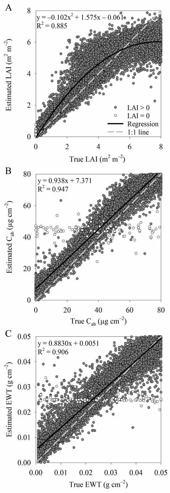
Figure 1.
True leaf area index (LAI, m2 m−2, (A)), chlorophyll content (Cab, µg cm−2, (B)), and equivalent water thickness (EWT, g cm−2, (C)) versus estimated values using the simulated test dataset. Estimations were compiled by an artificial neural network-based inversion of the radiative transfer model PROSAIL. Hyperspectral input data were used, and background soil spectra correction was included. Coefficients of linear or quadratic regression (a, b and c) as well as respective coefficients of determination (R2) are presented.
When LAI was 0, the estimations of Cab and EWT in Figure 1B,C showed random scattering around the respective mean values.
3.2. Estimating Wheat Traits
Table 3 provides an overview of data collected in field experiments on individual sampling dates in the 2019/2020 and 2020/21 seasons. It presents developmental stages as well as estimated marginal means and standard deviation values of PAI, NY, CWC, and AGDM for autumn- and spring-sown wheat across five nitrogen fertilization levels from 0 to 20 g N m−2.
Table 3.
Developmental stage (BBCH) as well as estimated marginal means (Mean) and standard deviation (SD) of plant area index (PAI, m2 m−2), nitrogen yield (NY, g m−2), canopy water content (CWC, g m−2), and above-ground dry matter (AGDM, g m−2) for autumn- and spring-sown wheat across five nitrogen fertilization levels from 0 to 20 g N m−2 on individual sampling dates in 2019/20 and 2020/21.
The mean PAI of the sampling dates ranged from 0.037 m2 m−2 (2019/20, spring-sowing, BBCH 11) to 3.751 m2 m−2 (2020/21, autumn-sowing, BBCH 57). The average AGDM of the sampling dates was the lowest in 2020/21 for spring-sown wheat at BBCH 10 (2.4 g m−2) and the highest also in 2020/21 for autumn-sown wheat at harvest, i.e., BBCH 89 (1151.9 g m−2). The mean NY of the sampling dates ranged from 0.13 g m−2 (2020/21, spring-sowing, BBCH 10) to 14.21 g m−2 (2020/21, autumn-sowing, BBCH 89). The lowest average CWC of the sampling dates was 7.4 g m−2 (2019/20, spring-sowing, BBCH 11), while the highest CWC was 2099.5 g m−2 (2020/21, autumn-sowing, BBCH 57).
Table 4 presents the results of estimating PAI, NY, and CWC using NDVI, NDRE, and four different RTM inversions during vegetative developmental stages from leaf development (BBCH 10) until the start of anthesis (BBCH 60). The models differed in the spectral resolution of input data and the inclusion or exclusion of background soil spectra correction. The traits PAI, NY, and CWC were estimated by the RTM inversion outputs LAI, LAI × Cab, and LAI × EWT, respectively. For model training based on the field experimental data of the 2020/21 season, regression types (linear, quadratic, and exponential), regression coefficients (a, b, c, and z) as well as R2 values are presented in Table 4. Model testing was based on the field experimental data of the 2019/20 season and included linear regression coefficients (a and b), R2 values, and RRMSE values. In all regression models, the estimated marginal means were used for model inputs and outputs.
Table 4.
Estimating plant area index (m2 m−2), nitrogen yield (g m−2) and canopy water content (g m−2) using normalized difference vegetation index (NDVI), normalized difference red-edge (NDRE), and artificial neural network-based radiative transfer model inversion (RTMI) during the vegetative developmental stages from leaf development (BBCH 10) to the start of anthesis (BBCH 60). The four RTMIs differed in the spectral resolution of input data (hyper- or multispectral) and the inclusion or exclusion of background soil spectra correction. The following RTMI outputs were used for respective trait estimations: leaf area index (LAI, m2 m−2), LAI multiplied by chlorophyll content (LAI × Cab, g m−2), and LAI multiplied by equivalent water thickness (LAI × EWT, g m−2). Vegetation index values and RTMI outputs were trained using the experimental data of the 2020/21 season. For training, regression type (linear, quadratic, or exponential), regression coefficients (a, b, c, and z), as well as coefficient of determination (R2) are presented. Estimations of PAI, NY, and CWC based on the trained models using vegetation indices and RTMI outputs were tested with the experimental data of the 2019/20 season. For model testing, linear regression coefficients (a and b), coefficients of determination, and relative root mean square error (RRMSE) are provided.
Regarding PAI, all models showed high R2 for model training ranging from 0.869 (RTM inversion with multispectral input data and no background soil spectra correction) to 0.964 (NDRE). In model testing, R2 values were lower, but still close to or above 0.8 for all models except for RTM inversion with multispectral input data and no background soil spectra correction (R2 = 0.521). The testing RRMSE was the lowest for RTM inversion with hyperspectral input data and background soil spectra correction (RRMSE = 17.9%, RMSE = 0.215 m2 m−2, mean = 1.200 m2 m−2). Other models that showed good testing PAI estimationss were NDVI (R2 = 0.893, RRMSE = 22.4%, RMSE = 0.269 m2 m−2) and RTM inversion with multispectral input data and background soil spectra correction (R2 = 0.792, RRMSE = 24.4%, RMSE = 0.293 m2 m−2).
The results on NY show high training R2 from 0.911 (RTM inversion with hyperspectral input data and no background soil spectra correction) to 0.970 (NDRE). In model testing, however, there were only two models with high R2 and low RRMSE. These were the RTM inversion with hyperspectral input data and background soil spectra correction (R2 = 0.908; RRMSE = 14.4%, RMSE = 0.608 g m−2, mean = 4.223 g m−2) and NDRE (R2 = 0.904; RRMSE = 23.0%, RMSE = 0.971 g m−2).
Lastly, in Table 4, CWC estimations also resulted in high training R2 for all models ranging from 0.826 (NDVI) to 0.944 (RTM inversion with hyperspectral input data and background soil spectra correction). In model testing, however, only the RTM inversion with hyperspectral input data and background soil spectra correction showed both high R2 (0.967) and low RRMSE (17.0%, RMSE = 82.2 g m−2, mean = 483.0 g m−2).
Figure 2 graphically presents the model training and testing of the RTM inversion with hyperspectral input data and background soil spectra correction for the estimation of PAI, NY, and CWC during the vegetative developmental stages.
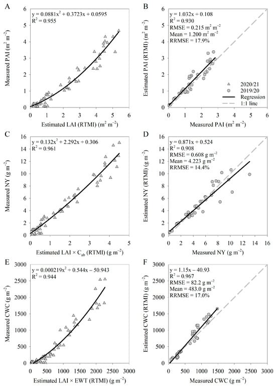
Figure 2.
Estimating plant area index (PAI, m2 m−2, (A,B)), nitrogen yield (NY, g m−2, (C,D)), and canopy water content (CWC, g m−2, (E,F)) using artificial neural network-based radiative transfer model inversion (RTMI) during the vegetative stages from leaf development (BBCH 10) to the start of anthesis (BBCH 60). This RTMI used hyperspectral input data and included background soil spectra correction. The outputs of RTMI were leaf area index (LAI, m2 m−2, (A)), LAI multiplied by chlorophyll content (LAI × Cab, g m−2, (C)), and LAI multiplied by equivalent water thickness (LAI × EWT, g m−2, (E)). For training, the field experimental data of the 2020/21 season was used (A,C,E). The model testing was performed with the field experimental data of the 2019/20 season (B,D,F).
Table 5 presents the results of PAI and CWC estimations throughout the growing season from leaf development (BBCH 10) until harvest (BBCH 89) using NDVI, NDRE, and the four different RTM inversions. For both PAI and CWC, one model featured the highest training and testing R2 as well as the lowest testing RRMSE. This was the RTM inversion with hyperspectral input data and background soil spectra correction. Estimations of PAI using the RTM inversion with hyperspectral input data and background soil spectra correction resulted in a training R2 of 0.922, a testing R2 of 0.845, and a testing RRMSE of 27.7% (RMSE = 0.364 m2 m−2, mean = 1.317 m2 m−2), while CWC estimations showed a training R2 of 0.927, a testing R2 of 0.884, and a testing RRMSE of 20.0% (RMSE = 115 g m−2, mean = 574 g m−2). All other models for PAI and CWC featured lower training and testing R2 values as well as higher testing RRMSE values. Figure 3 visually presents the training and testing of PAI and CWC estimations throughout the growing season based on the RTM inversion with hyperspectral input data and background soil spectra correction. Severe deviations from the 1:1 line in model testing for PAI and CWC estimations in Figure 3B,D occurred partially for data collected at harvest (BBCH 89).
Table 5.
Estimating plant area index (m2 m−2) and canopy water content (g m−2) using normalized difference vegetation index (NDVI), normalized difference red-edge (NDRE), and artificial neural network-based radiative transfer model inversion (RTMI) throughout the growing season from leaf development (BBCH 10) to harvest (BBCH 89). The four RTMIs differed in the spectral resolution of input data (hyper- or multispectral) and the inclusion or exclusion of background soil spectra correction. The following RTMI outputs were used for respective trait estimations: leaf area index (LAI, m2 m−2) and LAI multiplied by equivalent water thickness (LAI × EWT, g m−2). Vegetation index values and RTMI outputs were trained using the field experimental data of the 2020/21 season. For model training, regression type, regression coefficients (a, b, c, and z), as well as coefficient of determination (R2) are presented. Model testing was performed with the field experimental data of the 2019/20 season. For model testing, linear regression coefficients (a and b), coefficients of determination, and relative root mean square error (RRMSE) are provided.
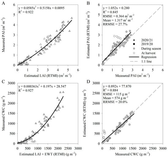
Figure 3.
Estimating plant area index (PAI, m2 m−2, (A,B)) and canopy water content (CWC, g m−2, (C,D)) using artificial neural network-based radiative transfer model inversion (RTMI) throughout the growing season from leaf development (BBCH 10) to harvest (BBCH 89). This RTMI used hyperspectral input data and included background soil spectra correction. Outputs of RTMI were leaf area index (LAI, m2 m−2, (A)) and LAI multiplied by equivalent water thickness (LAI × EWT, g m−2, (C)). For training, the field experimental data of the 2020/21 season was used (A,C). The model testing was performed with the field experimental data of the 2019/20 season (B,D).
Estimating NY from leaf development (BBCH 10) to harvest (BBCH 89) was tested; however, R2 values were low and RRMSE values were high for all models.
Finally, AGDM estimations throughout the growing season from leaf development (BBCH 10) to harvest (BBCH 89) were conducted based on PAD, NDVI integral, as well as LAD (Table 6). PAD was calculated using destructively measured PAI. LAD was calculated using LAI estimations based on the RTM inversion with hyperspectral input data and background soil spectra correction. Accordingly, the integral over time was also calculated for NDVI. Models were trained using the field experimental data of the 2020/21 season and tested using the field experimental data of the 2019/20 season. All three models, PAD, NDVI integral, and LAD, showed high training and testing R2 as well as low testing RRMSE. Training R2 values were similar ranging from 0.965 (RTM inversion-based LAD) to 0.972 (measured PAD). Testing R2 was the lowest for measured PAD (0.914) and highest for RTM inversion-based LAD (0.960). Testing RRMSE was 18.1% (RMSE = 77.0 g m−2, mean = 426.0 g m−2) for the measured PAD, 24.3% (RMSE = 103.3 g m−2) for NDVI integral, and 13.7% (RMSE = 58.6 g m−2) for RTM inversion-based LAD.
Table 6.
Estimating above-ground dry matter (AGDM, g m−2) throughout the growing season from leaf development (BBCH 10) to harvest (BBCH 89) using plant area duration (PAD, m2 m−2 d), integral of normalized difference vegetation index (NDVI) over time, as well as leaf area duration (LAD, m2 m−2). The latter was calculated with an artificial neural network-based radiative transfer model inversion (RTMI). This RTMI applied hyperspectral input data and background soil spectra correction. The RTMI output was leaf area index (LAI, m2 m−2). The destructively measured plant area index (PAI, m2 m−2) was used to calculate PAD. The integral over time was calculated for measured PAI, NDVI, as well as RTMI-based LAI. The integrals of PAI and LAI over time are PAD and LAD, respectively. Values of PAD, NDVI integral, and LAD were trained using the experimental data of the 2020/21 season. For training, regression type, regression coefficients (a, b, and c), as well as coefficient of determination (R2) are presented. Model testing was performed with the field experimental data of the 2019/20 season. For model testing, linear regression coefficients (a and b), coefficients of determination, and relative root mean square error (RRMSE) are provided.
The training and testing of the RTM inversion-based LAD model with hyperspectral input data and background soil spectra correction are presented visually in Figure 4.
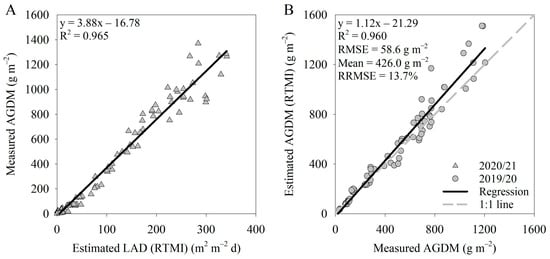
Figure 4.
Estimating above-ground dry matter (AGDM, g m−2) throughout the growing season from leaf development (BBCH 10) to harvest (BBCH 89) using artificial neural network-based radiative transfer model inversion (RTMI). This RTMI used hyperspectral input data and included background soil spectra correction. Leaf area duration (LAD, m2 m−2 d) is the integral of leaf area index (LAI, m2 m−2) over time. Values of LAI were estimated by the RTMI. For training, the field experimental data of the 2020/21 season was used (A). Model testing was performed with the field experimental data of the 2019/20 season (B).
4. Discussion
4.1. Radiative Transfer Model Inversion
The RTM inversion was successful for the relevant traits in this study, i.e., LAI, Cab, and EWT, as shown by high R2 (Table 2) and low RRMSE for the PROSAIL parameter estimations based on the simulated test dataset (Section 3.1.). Furthermore, the estimations of other PROSAIL parameters also featured high R2 in the simulated test dataset, e.g., Ccx, Cbp, ALIA, and LMA. These additional traits, however, could not be analyzed further, because no field experimental data on these traits were available.
The estimations of LAI based on a simulated test dataset were similar or superior to the results reported by Atzberger [19] (R2 = 0.85, RMSE = 0.59 m2 m−2), Weiss and Baret [22] (RMSE = 0.89 m2 m−2), Bacour et al. [46] (R2 = 0.80, RMSE = 1.15 m2 m−2), and Verger et al. [47] (RMSE = 0.91 m2 m−2). Furthermore, Atzberger [19] showed similar performance for the estimations of Cab (R2 = 0.83, RMSE = 7.8 µg cm−2) and EWT (R2 = 0.92, RMSE = 0.003 g cm−2) based on the simulated test data. These studies, however, simulated varying spectral resolutions and did not limit their dataset to a specific crop. In this paper, the spectral resolution was limited to the spectral range from 400 to 1000 nm in 1 nm increments, i.e., hyperspectral, or Sentinel-2A bands 1 to 9, including 8A, i.e., multispectral.
The use of hyperspectral input data resulted in superior trait estimations compared to multispectral input data (Table 2). This is in accordance with Baret and Buis [9], Atzberger et al. [10] and Weiss et al. [48], who reason that an increase in the number of spectral bands can improve trait estimations in terms of noise sensitivity, robustness, generalization, and reproducibility.
Furthermore, RTM inversions excluding the background soil spectra correction featured a superior R2 compared to RTM inversions including the background soil spectra correction (Table 2). The two simulated datasets, i.e., one including and one excluding background soil spectra correction, drastically differed in their variability in background soil spectra. The standard soil spectrum in the simulated dataset excluding background correction was generated using a single default soil spectrum for all observations and a randomly selected soil brightness factor αsoil. In comparison, the soil spectrum in the simulated dataset including background soil spectra correction was randomly selected from the 3717 highly varying soil spectra of the ICRAF-ISRIC Soil MIR Spectral Library [40] for each observation. Therefore, the variability in soil spectra was substantially higher in the simulated dataset including background soil spectra correction. The ANN models that were trained on the two variants of the simulated dataset were of identical structure, i.e., number of layers and neurons. Therefore, the model tested on the simulated dataset of lower variability, i.e., excluding background correction, showed superior performance compared to the model tested on the highly variable simulated dataset, i.e., including background correction.
Furthermore, Cab and EWT could not be estimated when LAI was 0 in the simulated test dataset. In these cases, the reflectance spectra were only dependent on the underlying soil spectra. Thus, the resulting estimations for Cab and EWT defaulted to their respective mean values in the simulated dataset (Figure 1).
4.2. Estimating Wheat Traits
The empirically collected data showed high variation in PAI, NY, CWC, and AGDM (Table 3) due to two distinct sowing times, autumn- and spring-sowing, two seasons with substantially differing weather conditions, 2019/20 and 2020/21, as well as five nitrogen fertilization rates from 0 to 20 g N m−2 and a high number of sampling dates within seasons. Therefore, the available field experimental data were a suitable, highly diverse empirical dataset for model training and testing.
The RTM inversion with hyperspectral input data and background soil spectra correction was the best model for the estimation of PAI, NY, and CWC during the vegetative stage from BBCH 10 to BBCH 60: PAI: train R2 = 0.955, test R2 = 0.930, RRMSE = 17.9%, RMSE = 0.215 m2 m−2, mean = 1.200 m2 m−2; NY: train R2 = 0.961, test R2 = 0.908, RRMSE: 14.4%, RMSE = 0.608 g m−2, mean = 4.223 g m−2; CWC: train R2 = 0.944, test R2 = 0.967, RRMSE: 17.0%, RMSE = 82.2 g m−2, and mean = 483.0 g m−2 (Table 4). These trait estimation results were similar or superior compared to the literature. Herrmann et al. [49], for example, estimated LAI in wheat during the vegetative stage using Partial Least Squares Regression based on Sentinel-2 bands with an R2 of 0.903 and a RMSE of 0.62 m2 m−2. Estimations of NY in wheat during the vegetative stage were conducted by Fitzgerald et al. [44] (R2 = 0.97, RMSE = 0.65 g m−2) and Palka et al. [8] (R2 = 0.9, RMSE = 1.84 g m−2) using the CCCI-CNI approach. Zhang et al. [50] reported CWC estimations in wheat throughout the growing season using the vegetation index NDWI (Normalized Difference Water Index) with an R2 of 0.68 and an RMSE of 148 g m−2.
Other RTM inversions in this study showed worse estimations of PAI, NY, and CWC for the empirical test dataset. For RTM inversions with multispectral input data, the decrease in model performance can be attributed to the reduction in spectral resolution and thus lower noise sensitivity, robustness, generalization, and reproducibility [9,10,48]. The inversions of the RTM without background soil spectra correction were not able to handle the highly varying soil spectra among sampling dates in an adequate way, which resulted in worse trait estimations. Weiss and Baret [22] as well as Danner et al. [24] also highlighted the importance of accounting for background soil spectra variation in RTM inversion. Nevertheless, PAI estimations using the RTM inversion with multispectral data and background soil spectra correction were adequate (train R2 = 0.922, test R2 = 0.792, RRMSE = 24.4%, RMSE = 0.293 m2 m−2, mean = 1.200 m2 m−2) (Table 4).
The simple approach using vegetation indices showed promising trait estimations during the vegetative stage based on the empirical test dataset, e.g., PAI estimations using NDVI (train R2 = 0.915, test R2 = 0.893, RRMSE = 22.4%, RMSE = 0.269 m2 m−2, mean = 1.200 m2 m−2) and NY estimations using NDRE (train R2 = 0.970, test R2 = 0.904, RRMSE = 23.0%, RMSE = 0.971 g m−2, mean = 4.223 g m−2). Estimations of CWC using the vegetation index approach, however, showed poor results.
The best model to estimate PAI and CWC from BBCH 10 to harvest (BBCH 89) was also the RTM inversion with hyperspectral input data and soil correction (PAI: train R2 = 0.922, test R2 = 0.845, RRMSE = 27.7%, RMSE = 0.364 m2 m−2, mean = 1.317 m2 m−2; CWC: train R2 = 0.927, test R2 = 0.884, RRMSE = 20.0%, RMSE = 115 g m−2, mean = 574 g m−2) (Table 5). Model performance, however, was generally worse compared to estimations limited to the vegetative stage (BBCH 10 to 60). Nevertheless, the performance of this model, i.e., hyperspectral input data and inclusion of the background soil spectra correction, was substantially better than all other models tested in this study. Other models based on vegetation indices and RTM inversions using multispectral input data or excluding background soil spectra correction featured a lower performance, especially in model testing. In Figure 3B,D, estimations at harvest (BBCH 89) showed severe deviations from the 1:1 line in model testing for PAI and CWC.
The presented estimations on PAI and CWC throughout the season were similar or superior to the results reported in the literature: Atzberger et al. [51], for example, conducted an ANN-based RTM inversion using hyperspectral input from 450 to 2500 nm data to estimate LAI (R2 = 0.86%, RMSE = 0.83 m2 m−2) in wheat throughout the growing season. Vuolo et al. [52] reported LAI estimations using RTM inversion based on Sentinel-2 bands across different crops with an R2 of 0.83 and an RMSE of 0.32 m2 m−2. Pan et al. [53] conducted trait estimations in wheat throughout the season using a look-up table-based RTM inversion approach on Sentinel-2 bands resulting in an RRMSE of 11% for LAI and 32% for CWC. Wu et al. [54] estimated CWC in wheat throughout the season using vegetation indices based on multispectral data. The vegetation index NDWI1940 resulted, for example, in CWC estimations with an R2 of 0.83.
The estimation of NY throughout the growing season (BBCH 10 to 89) was evaluated; however, the results were generally poor for all models. This can be explained by the change in the allocation of nitrogen from the vegetative to the generative stage. From germination to flowering, the available nitrogen is generally used to produce chlorophyll, which can be detected spectrally. From the start of the generative stage onwards, however, the nitrogen in chlorophyll is translocated to the grains for storage proteins. Thus, NY can be estimated by the chlorophyll content during the vegetative stage; however, the chlorophyll content is not a good predictor of NY during the generative stage [55].
Finally, there were three models tested for estimating AGDM: measured PAD, NDVI integral, and RTM inversion-based LAD. All three models showed a suitable performance; however, the results of the RTM inversion with hyperspectral input data and background soil spectra correction (RTM inversion-based LAD) were superior to the other models tested in this study (train R2 = 0.965, test R2 = 0.960, RRMSE = 13.7%, RMSE = 58.6 g m−2, mean = 426.0 g m−2). This is especially noteworthy, since one of the alternative models was based on destructively measured PAI values (train R2 = 0.972, test R2 = 0.914, RRMSE = 18.1%). The comparatively simple NDVI integral approach also showed good results for AGDM estimations (train R2 = 0.969, test R2 = 0.927, RRMSE = 24.3%). In comparison, Tucker et al. [56] were among the first to correlate spectral data with AGDM in wheat and achieved an R2 of 0.79. Mistele and Schmidhalter [57] determined dry matter yields in maize using curvilinear models between spectral indices and AGDM with R2 ranging from 0.67 to 0.91 in three seasons. Fabbri et al. [58] tested various vegetation indices to estimate AGDM in durum wheat. The best performing index for AGDM was EVI2 (R2 = 0.951, RRMSE = 17.9%) during the vegetative stage.
The presented model performances are promising; nevertheless, it needs to be mentioned that these models also feature certain limitations. The selected RTM PROSAIL is a basic RTM that features a simplified description of canopy architecture compared to more complex RTMs [25]. Furthermore, the field experimental dataset is limited in the following aspects: limited data variability, i.e., solely one crop (wheat) was investigated in one region (Eastern Austria) in two seasons; limited dataset size, i.e., a modest number of data points; and limitations of the applied spectral sensor, i.e., no spatial variation and limited spectral resolution from 400 to 1000 nm. In the context of CWC estimations, for example, the spectral reflectance above 1000 nm is of substantial importance [54]. To offset the limitation of the small field experimental dataset, a simulated dataset based on an RTM inversion was introduced in this study. The extensive use of simulated data as well as the previously mentioned aspects on the limitations of the RTM PROSAIL and the field experimental dataset, however, limit the generalizability of the proposed models.
Although the proposed models show certain limitations, they nevertheless resulted in suitable model performances for estimating PAI, CWC, and AGDM throughout the growing season as well as NY from leaf development (BBCH 10) to anthesis (BBCH 60) for wheat in Eastern Austria. The presented models can be used in future studies for quick and non-destructive measurements of PAI, CWC, NY, and AGDM based on spectral measurements of wheat in Eastern Austria during the aforementioned developmental stages. This can reduce the required workload drastically. Furthermore, when applied jointly, the proposed models for estimating PAI, CWC, NY, and AGDM can improve the evaluation of stress conditions in wheat canopies, e.g., nitrogen deficiencies and drought. Additionally, the models and methods proposed in this study can be used as templates for setting up models for additional wheat cultivars, crops, regions, or target traits in the future. Furthermore, the approach presented in this study can be adapted to establish models for different spectral resolutions and spatial resolutions of other sensors that can be mounted on a tripod or a tractor for proximal measurements, on a drone, an airplane, or also satellites. The proposed methodology can also be advanced by applying more complex RTMs, e.g., 4SAIL2 [59,60] and SCOPE [61], or different machine learning algorithms, e.g., random forests, support vector machines, more complex ANNs, and gradient boosting or convolution neural networks for object detection. More complex methodologies can additionally introduce a comparison of performances across different models or investigate the model interpretability, e.g., explainable artificial intelligence [62].
5. Conclusions
The results indicate that both differences in spectral resolution, i.e., hyperspectral versus multispectral, as well as the inclusion versus exclusion of background soil spectra correction substantially affected the model estimations of the simulated dataset as well as the field experimental dataset.
Many RTM inversion-based models presented in this study resulted in suitable estimations of wheat traits. Thus, the approach proposed by Reinosch et al. [14], which combines empirically collected data with mechanistic models, e.g., RTMs, was successful in building models based on machine learning with a limited experimental dataset. The RTM inversion with hyperspectral input data and background soil spectra correction was the best among all tested models to estimate PAI, NY, and CWC during the vegetative stages (BBCH 10 to 60) as well as PAI and CWC throughout the growing season (BBCH 10 to 89). Additionally, this model was also the best for estimating AGDM based on the integral of estimated LAI values over days, i.e., the LAD. Furthermore, this model was equivalent or superior compared to similar trait estimation results reported in the literature.
With this study, a promising new model to estimate PAI, NY, CWC, and AGDM was established. This model was specifically designed for the available spectroradiometer with a spectral resolution from 400 to 1000 nm in 1 nm increments. Going forward, this combination of sensor and model can now be applied in wheat field experiments to reduce labor and costs for analyzing PAI, NY, CWC, and AGDM. Nevertheless, the simple approach using vegetation indices also showed good results, especially for the estimation of PAI and NY during vegetative stages (BBCH 10 to 60) as well as the estimation of AGDM using NDVI integral. The estimations of PAI throughout the growing season and CWC in general, however, were substantially worse using vegetation indices compared to the RTM inversion with hyperspectral input data and including background soil spectra correction.
Many models presented in this study, both vegetation index as well as RTM inversion-based, provided suitable estimations of the relevant wheat traits PAI, NY, CWC, and AGDM for various applications in, for example, agronomy, breeding, and crop sciences in general.
Author Contributions
Conceptualization, L.J.K., H.-P.K., S.R., P.W., P.E., T.N., N.B. and R.W.N.; methodology, L.J.K., H.-P.K., S.R., P.W. and R.W.N.; software, L.J.K., H.-P.K., S.R., P.W., N.B. and R.W.N.; validation, L.J.K., H.-P.K. and R.W.N.; formal analysis, L.J.K., H.-P.K., S.R., P.W. and R.W.N.; investigation, L.J.K., H.-P.K., A.K.-K. and R.W.N.; resources, L.J.K., H.-P.K., P.E., T.N., N.B. and R.W.N.; data curation, L.J.K., H.-P.K., S.R., P.W., J.B., G.M., G.M. and R.W.N.; writing—original draft preparation, L.J.K.; writing—review and editing, L.J.K., H.-P.K., S.R., P.W., P.E., J.B., G.M., T.N., A.K.-K., N.B. and R.W.N.; visualization, L.J.K., H.-P.K. and R.W.N.; supervision, H.-P.K., T.N., A.K.-K. and R.W.N.; project administration, L.J.K., H.-P.K., T.N., N.B. and R.W.N.; funding acquisition, H.-P.K., T.N., N.B. and R.W.N. All authors have read and agreed to the published version of the manuscript.
Funding
This research was funded by the project “DiLaAg—Digitalization and Innovation Laboratory in Agricultural Sciences” of the private foundation “Forum Morgen, Austria” and the Federal State of Lower Austria.
Data Availability Statement
The raw data supporting the conclusions of this article will be made available by the authors on request.
Acknowledgments
We thank Ivica Simonovic and Johannes Kemetter for managing the field experiments; our student assistants Anna Hofer, Caroline Huber, Laura Sturm, and Vincent Aubry for their assistance in the field and laboratory; as well as Craig Jackson for his field assistance and for conducting laboratory analyses.
Conflicts of Interest
The authors declare no conflicts of interest.
References
- Myers, V.I.; Allen, W.A. Electrooptical Remote Sensing Methods as Nondestructive Testing and Measuring Techniques in Agriculture. Appl. Opt. 1968, 7, 1819–1838. [Google Scholar] [CrossRef] [PubMed]
- Wiegand, C.L.; Richardson, A.J.; Kanemasu, E.T. Leaf Area Index Estimates for Wheat from LANDSAT and Their Implications for Evapotranspiration and Crop Modeling. Agron. J. 1979, 71, 336–342. [Google Scholar] [CrossRef]
- Khanal, S.; Kushal, K.C.; Fulton, J.P.; Shearer, S.; Ozkan, E. Remote Sensing in Agriculture—Accomplishments, Limitations, and Opportunities. Remote Sens. 2020, 12, 3783. [Google Scholar] [CrossRef]
- Baret, F.; Guyot, G. Potentials and limits of vegetation indices for LAI and APAR assessment. Remote Sens. Environ. 1991, 35, 161–173. [Google Scholar] [CrossRef]
- Haboudane, D.; Miller, J.R.; Pattey, E.; Zarco-Tejada, P.J.; Strachan, I.B. Hyperspectral vegetation indices and novel algorithms for predicting green LAI of crop canopies: Modeling and validation in the context of precision agriculture. Remote Sens. Environ. 2004, 90, 337–352. [Google Scholar] [CrossRef]
- Marti, J.; Bort, J.; Slafer, G.A.; Araus, J.L. Can wheat yield be assessed by early measurements of Normalized Difference Vegetation Index? Ann. Appl. Biol. 2007, 150, 253–257. [Google Scholar] [CrossRef]
- Mulla, D.J. Twenty-five years of remote sensing in precision agriculture: Key advances and remaining knowledge gaps. Biosyst. Eng. 2013, 114, 358–371. [Google Scholar] [CrossRef]
- Palka, M.; Manschadi, A.M.; Koppensteiner, L.J.; Neubauer, T.; Fitzgerald, G.J. Evaluating the performance of the CCCI-CNI index for estimating N status of winter wheat. Eur. J. Agron. 2021, 130, 126346. [Google Scholar] [CrossRef]
- Baret, F.; Buis, S. Estimating canopy characteristics from remote sensing observations: Review of methods and associated problems. In Advances in Land Remote Sensing; Springer: Dordrecht, The Netherlands, 2008; pp. 173–201. [Google Scholar]
- Atzberger, C.; Darvishzadeh, R.; Immitzer, M.; Schlerf, M.; Skidmore, A.; le Maire, G. Comparative analysis of different retrieval methods for mapping grassland leaf area index using airborne imaging spectroscopy. Int. J. Appl. Earth Obs. Geoinf. 2015, 43, 19–31. [Google Scholar] [CrossRef]
- Bian, C.; Shi, H.; Wu, S.; Zhang, K.; Wei, M.; Zhao, Y.; Sun, Y.; Zhuang, H.; Zhang, X.; Chen, S. Prediction of Field-Scale Wheat Yield Using Machine Learning Method and Multi-Spectral UAV Data. Remote Sens. 2022, 14, 1474. [Google Scholar] [CrossRef]
- Cheng, E.; Zhang, B.; Peng, D.; Zhong, L.; Yu, L.; Liu, Y.; Xiao, C.; Li, C.; Li, X.; Chen, Y.; et al. Wheat yield estimation using remote sensing data based on machine learning approaches. Front. Plant Sci. 2022, 13, 1090970. [Google Scholar] [CrossRef] [PubMed]
- van Klompenburg, T.; Kassahun, A.; Catal, C. Crop yield prediction using machine learning: A systematic literature review. Comput. Electron. Agric. 2020, 177, 105709. [Google Scholar] [CrossRef]
- Reinosch, N.; Münzberg, A.; Martini, D.; Niehus, A.; Seuring, L.; Troost, C.; Kumar Srivastava, R.; Berger, T.; Streck, T.; Bernardi, A. SIMLEARN—Ontologiegestützte Integration von Simulationsmodellen, Systemen für maschinelles Lernen und Planungsdaten. In 43. GIL-Jahrestagung, Resiliente Agri-Food-Systeme; Gesellschaft für Informatik e.V.: Bonn, Germany, 2023; pp. 477–482. ISBN 978-3-88579-724-1. [Google Scholar]
- Monteith, J.L. Light Distribution and Photosynthesis in Field Crops. Ann. Bot. 1965, 29, 17–37. Available online: https://www.jstor.org/stable/42908627 (accessed on 22 August 2022). [CrossRef]
- Berger, K.; Atzberger, C.; Danner, M.; D’Urso, G.; Mauser, W.; Vuolo, F.; Hank, T. Evaluation of the PROSAIL Model Capabilities for Future Hyperspectral Model Environments: A Review Study. Remote Sens. 2018, 10, 85. [Google Scholar] [CrossRef]
- Richter, K.; Atzberger, C.; Vuolo, F.; D’Urso, G. Evaluation of Sentinel-2 Spectral Sampling for Radiative Transfer Model Based LAI Estimation of Wheat, Sugar Beet, and Maize. IEEE J. Sel. Top. Appl. Earth Obs. Remote Sens. 2011, 4, 458–464. [Google Scholar] [CrossRef]
- Locherer, M.; Hank, T.; Danner, M.; Mauser, W. Retrieval of Seasonal Leaf Area Index from Simulated EnMAP Data through Optimized LUT-Based Inversion of the PROSAIL Model. Remote Sens. 2015, 7, 10321–10346. [Google Scholar] [CrossRef]
- Atzberger, C. Object-based retrieval of biophysical canopy variables using artificial neural nets and radiative transfer models. Remote Sens. Environ. 2004, 93, 53–67. [Google Scholar] [CrossRef]
- Duveiller, G.; Weiss, M.; Baret, F.; Defourny, P. Retrieving wheat Green Area Index during the growing season from optical time series measurements based on neural network radiative transfer inversion. Remote Sens. Environ. 2011, 115, 887–896. [Google Scholar] [CrossRef]
- Zhu, J.; Lu, J.; Li, W.; Wang, Y.; Jiang, J.; Cheng, T.; Zhu, Y.; Cao, W.; Yao, X. Estimation of canopy water content for wheat through combining radiative transfer model and machine learning. Field Crops Res. 2023, 302, 109077. [Google Scholar] [CrossRef]
- Weiss, M.; Baret, F.; Jay, S. S2ToolBox Level 2 Products: LAI, FAPAR, FCOVER; INRAE: Paris, France, 2016. [Google Scholar]
- Huete, A.R. A soil-adjusted vegetation index (SAVI). Remote Sens. Environ. 1988, 25, 295–309. [Google Scholar] [CrossRef]
- Danner, M.; Berger, K.; Wocher, M.; Mauser, W.; Hank, T. Retrieval of Biophysical Crop Variables from Multi-Angular Canopy Spectroscopy. Remote Sens. 2017, 9, 726. [Google Scholar] [CrossRef]
- Jacquemoud, S.; Verhoef, W.; Baret, F.; Bacour, C.; Zarco-Tejada, P.J.; Asner, G.P.; François, C.; Ustin, S.L. PROSPECT + SAIL models: A review of use for vegetation characterization. Remote Sens. Environ. 2009, 113, 56–66. [Google Scholar] [CrossRef]
- Koppensteiner, L.J.; Kaul, H.-P.; Piepho, H.-P.; Barta, N.; Euteneuer, P.; Bernas, J.; Klimek-Kopyra, A.; Gronauer, A.; Neugschwandtner, R.W. Yield and yield components of facultative wheat are affected by sowing time, nitrogen fertilization and environment. Eur. J. Agron. 2022, 140, 126591. [Google Scholar] [CrossRef]
- Bernas, J.; Koppensteiner, L.J.; Tichá, M.; Kaul, H.-P.; Klimek-Kopyra, A.; Euteneuer, P.; Moitzi, G.; Neugschwandtner, R.W. Optimal environmental design of nitrogen application rate for facultative wheat using life cycle assessment. Eur. J. Agron. 2023, 146, 126813. [Google Scholar] [CrossRef]
- Moitzi, G.; Koppensteiner, L.J.; Klimek-Kopyra, A.; Bernas, J.; Kaul, H.-P.; Wagentristl, H.; Euteneuer, P.; Neugschwandtner, R.W. Effects of sowing date and nitrogen applications on the energy efficiency of facultative wheat (Triticum aestivum L.) in a Pannonian environment. Heliyon 2024, 10, e37923. [Google Scholar] [CrossRef]
- Neugschwandtner, R.W.; Liebhard, P.; Kaul, H.-P.; Wagentristl, H. Soil chemical properties as affected by tillage and crop rotation in a long-term field experiment. Plant Soil Environ. 2014, 60, 57–62. [Google Scholar] [CrossRef]
- Witzenberger, A.; Hack, H.; van den Boom, T. Erläuterungen zum BBCH-Dezimal-Code für die Entwicklungsstadien des Getreides—Mit Abbildungen [Commentary to the BBCH-decimal-code for growth stages of cereals—With images]. Gesunde Pflanz. 1989, 41, 384–388. (In German) [Google Scholar]
- Meier, U.; Bleiholder, H.; Buhr, L.; Feller, C.; Hack, H.; Hess, M.; Lancashire, P.D.; Schnock, U.; Stauss, R.; van den Boom, T.; et al. The BBCH system to coding the phenological growth stages of plants—History and publications. J. Kult. 2009, 61, 41–52. [Google Scholar] [CrossRef]
- Winkler, R.; Botterbrodt, S.; Rabe, E.; Lindhauer, M.G. Stickstoff-/Proteinbestimmung mit der Dumas-Methode in Getreide und Getreideprodukten [Nitrogen and protein determination using the Dumas method in cereal and cereal products]. Getreide Mehl Brot 2000, 54, 86–91. (In German) [Google Scholar]
- Jacquemoud, S.; Baret, F. PROSPECT: A model of leaf optical properties spectra. Remote Sens. Environ. 1990, 34, 75–91. [Google Scholar] [CrossRef]
- Feret, J.-B.; François, C.; Asner, G.P.; Gitelson, A.A.; Martin, R.E.; Bidel, L.P.R.; Ustin, S.L.; le Maire, G.; Jacquemoud, S. PROSPECT-4 and 5: Advances in the leaf optical properties model separating photosynthetic pigments. Remote Sens. Environ. 2008, 112, 3030–3043. [Google Scholar] [CrossRef]
- Kuusk, A. The Hot Spot Effect in Plant Canopy Reflectance. In Photon-Vegetation Interactions: Applications in Optical Remote Sensing and Plant Ecology; Myneni, R.B., Ross, J., Eds.; Springer: Berlin/Heidelberg, Germany, 1991; pp. 139–159. [Google Scholar]
- Spitters, C.J.T.; Toussaint, H.A.J.M.; Goudriaan, J. Separating the diffuse and direct component of global radiation and its implications for modeling canopy photosynthesis Part I. Components of incoming radiation. Agric. For. Meteorol. 1986, 38, 217–229. [Google Scholar] [CrossRef]
- Richter, K.; Vuolo, F.; D’Urso, G.; Palladino, M. Evaluation of near-surface soil water status through the inversion of soil-canopy radiative transfer models in the reflective optical domain. Int. J. Remote Sens. 2012, 33, 5473–5491. [Google Scholar] [CrossRef]
- Kong, W.P.; Huang, W.J.; Zhou, X.F.; Song, X.Y.; Casa, R. Estimation of carotenoid content at the canopy scale using the carotenoid triangle ratio index from in situ and simulated hyperspectral data. J. Appl. Remote Sens. 2016, 10, 026035. [Google Scholar] [CrossRef]
- Van Reeuwjik, L.P. Procedure for Soil Analysis, 6th ed.; ISRIC: Wageningen, The Netherlands, 2002. [Google Scholar]
- SoilSpec4GG Open Soil Spectral Library Explorer. Soil Spectroscopy 4 Global Good. 2022. Available online: https://explorer.soilspectroscopy.org/ (accessed on 7 July 2022).
- Stanford University. CS231n Deep Learning for Computer Vision; Stanford University: Stanford, CA, USA, 2024; Available online: https://cs231n.github.io/neural-networks-1/ (accessed on 3 January 2025).
- ESA (European Space Agency). Sentinel-2 Spectral Response Functions (S2-SRF), Version: 3.2. 10 October 2023. Available online: https://sentinels.copernicus.eu/documents/d/sentinel/s2-srf_cope-gseg-eopg-tn-15-0007_3-2 (accessed on 7 January 2024).
- Akanbi, O.; Amiri, I.; Fazeldehkordi, E. Chapter 4—Feature Extraction. In A Machine-Learning Approach to Phishing Detection and Defense; Akanbi, O., Amiri, I., Fazeldehkordi, E., Eds.; Syngress: Rockland, MA, USA, 2015; pp. 45–54. [Google Scholar] [CrossRef]
- Fitzgerald, G.; Rodriguez, D.; O’Leary, G. Measuring and predicting canopy nitrogen nutrition in wheat using a spectral index —The canopy chlorophyll content index (CCCI). Field Crops Res. 2010, 116, 318–324. [Google Scholar] [CrossRef]
- Piepho, H.P.; Büchse, A.; Emrich, K. A Hitchhiker’s Guide to Mixed Models for Randomized Experiments. J. Agron. Crop Sci. 2003, 189, 310–322. [Google Scholar] [CrossRef]
- Bacour, C.; Baret, F.; Béal, D.; Weiss, M.; Pavageau, K. Neural network estimation of LAI, fAPAR, fCover and LAI×Cab, from top of canopy MERIS reflectance data: Principles and validation. Remote Sens. Environ. 2006, 105, 313–325. [Google Scholar] [CrossRef]
- Verger, A.; Baret, F.; Camacho, F. Optimal modalities for radiative transfer-neural network estimation of canopy biophysical characteristics: Evaluation over an agricultural area with CHRIS/PROBA observation. Remote Sens. Environ. 2011, 115, 415–426. [Google Scholar] [CrossRef]
- Weiss, M.; Baret, F.; Myneni, R.B.; Pragnere, A.; Knyazikhin, Y. Investigation of a model inversion technique to estimate canopy biophysical variables from spectral and directional reflectance data. Agronomie 2000, 20, 3–22. [Google Scholar] [CrossRef]
- Herrmann, I.; Pimstein, A.; Karnieli, A.; Cohen, Y.; Alchanatis, V.; Bonfil, D.J. LAI assessment of wheat and potato crops by Venμs and Sentinel-2 bands. Remote Sens. Environ. 2011, 115, 2141–2151. [Google Scholar] [CrossRef]
- Zhang, C.; Pattey, E.; Liu, J.; Cai, H.; Shang, J.; Dong, T. Retrieving leaf and canopy water content of winter wheat using vegetation water indices. IEEE J. Sel. Top. Appl. Earth Obs. Remote Sens. 2017, 11, 112–126. [Google Scholar] [CrossRef]
- Atzberger, C.; Jarmer, T.; Schlerf, M.; Kötz, B.; Werner, W. Retrieval of wheat bio-physical attributes from hyperspectral data and SAILH+PROSPECT radiative transfer model. In Proceedings of the 3rd EARSeL Workshop Imaging Spectroscopy, Oberpfaffenhof, Germany, 13–16 May 2003. [Google Scholar]
- Vuolo, F.; Zółtak, M.; Pipitone, C.; Zappa, L.; Wenng, H.; Immitzer, M.; Weiss, M.; Baret, F.; Atzberger, C. Data service platform for Sentinel-2 surface reflectance and value-added products: System use and examples. Remote Sens. 2016, 8, 938. [Google Scholar] [CrossRef]
- Pan, H.; Chen, Z.; Ren, J.; Li, H.; Wu, S. Modeling winter wheat leaf area index and canopy water content with three different approaches using sentinel-2 multispectral instrument data. IEEE J. Sel. Top. Appl. Earth Obs. Remote Sens. 2018, 12, 482–492. [Google Scholar] [CrossRef]
- Wu, C.; Niu, Z.; Tang, Q. Predicting vegetation water content in wheat using normalized difference water indices derived from ground measurements. J. Plant Res. 2009, 122, 317–326. [Google Scholar] [CrossRef]
- Simpson, R.J.; Lambers, H.; Dalling, M.J. Nitrogen Redistribution during Grain Growth in Wheat (Triticum aestivum L.): IV. Development of a Quantitative Model of the Translocation of Nitrogen to the Grain. Plant Physiol. 1983, 71, 7–14. [Google Scholar] [CrossRef] [PubMed]
- Tucker, C.J.; Holben, B.N.; Elgin, J.H.; McMurtrey, J.E. Remote sensing of total dry-matter accumulation in winter wheat. Remote Sens. Environ. 1981, 11, 171–189. [Google Scholar] [CrossRef]
- Mistele, B.; Schmidhalter, U. Spectral measurements of the total aerial N and biomass dry weight in maize using a quadrilateral-view optic. Field Crops Res. 2008, 106, 94–103. [Google Scholar] [CrossRef]
- Fabbri, C.; Mancini, M.; dalla Marta, A.; Orlandini, S.; Napoli, M. Integrating satellite data with a nitrogen nutrition curve for precision top-dress fertilization of durum wheat. Eur. J. Agron. 2020, 120, 126148. [Google Scholar] [CrossRef]
- Verhoef, W.; Bach, H. Coupled soil–leaf-canopy and atmosphere radiative transfer modeling to simulate hyperspectral multi-angular surface reflectance and TOA radiance data. Remote Sens. Environ. 2007, 109, 166–182. [Google Scholar] [CrossRef]
- Verhoef, W.; Jia, L.; Xiao, Q.; Su, Z. Unified Optical-Thermal Four-Stream Radiative Transfer Theory for Homogeneous Vegetation Canopies. IEEE Trans. Geosci. Remote Sens. 2007, 45, 1808–1822. [Google Scholar] [CrossRef]
- van der Tol, C.; Verhoef, W.; Timmermans, J.; Verhoef, A.; Su, Z. An integrated model of soil-canopy spectral radiances, photosynthesis, fluorescence, temperature and energy balance. Biogeosciences 2009, 6, 3109–3129. [Google Scholar] [CrossRef]
- Holzinger, A. Explainable AI (ex-AI). Inform. Spektrum 2018, 41, 138–143. [Google Scholar] [CrossRef]
Disclaimer/Publisher’s Note: The statements, opinions and data contained in all publications are solely those of the individual author(s) and contributor(s) and not of MDPI and/or the editor(s). MDPI and/or the editor(s) disclaim responsibility for any injury to people or property resulting from any ideas, methods, instructions or products referred to in the content. |
© 2025 by the authors. Licensee MDPI, Basel, Switzerland. This article is an open access article distributed under the terms and conditions of the Creative Commons Attribution (CC BY) license (https://creativecommons.org/licenses/by/4.0/).