A Robust Multispectral Reconstruction Network from RGB Images Trained by Diverse Satellite Data and Application in Classification and Detection Tasks

Abstract

Multispectral images contain richer spectral signatures than easily available RGB images, for which they are promising to contribute to information perception. However, the relatively high cost of multispectral sensors and lower spatial resolution limit the widespread application of multispectral data, and existing reconstruction algorithms suffer from a lack of diverse training datasets and insufficient reconstruction accuracy. In response to these issues, this paper proposes a novel and robust multispectral reconstruction network from low-cost natural color RGB images based on free available satellite images with various land cover types. First, to supplement paired natural color RGB and multispectral images, the Houston hyperspectral dataset was used to train a convolutional neural network Model-TN for generating natural color RGB images from true color images combining CIE standard colorimetric system theory. Then, the EuroSAT multispectral satellite images for eight land cover types were selected to produce natural RGB using Model-TN as training image pairs, which were input into a residual network integrating channel attention mechanisms to train the multispectral images reconstruction model, Model-NM. Finally, the feasibility of the reconstructed multispectral images is verified through image classification and target detection. There is a small mean relative absolute error value of 0.0081 for generating natural color RGB images, which is 0.0397 for reconstructing multispectral images. Compared to RGB images, the accuracies of classification and detection using reconstructed multispectral images have improved by 16.67% and 3.09%, respectively. This study further reveals the potential of multispectral image reconstruction from natural color RGB images and its effectiveness in target detection, which promotes low-cost visual perception of intelligent unmanned systems.

1. Introduction

Multispectral images contain abundant spectral information and show an exceptional ability to describe the spectral characteristics of objects, playing a significant role in military, remote sensing, agriculture, medical fields, etc. Studies have shown that multispectral images contain additional spectral information compared to RGB images and can better characterize the differences between different objects, optimizing the accuracy of image classification [1,2,3,4]. Benefited from rich spectral information, multispectral images generally show superior application performance in many fields compared to RGB images [5]. However, there is a high cost for obtaining multispectral images using professional cameras, which is not conducive to the widespread application of multispectral images. Therefore, there is an urgent need to develop a method to obtain high-quality multispectral images at a low cost.

Currently, spectral reconstruction technology is commonly used to obtain multispectral images at a low cost. Spectral reconstruction, also known as spectral super-resolution, refers to the process of obtaining high-spectral images or multispectral images with rich spectral information from RGB images that have less spectral information. Spectral reconstruction technology is mainly divided into traditional spectral reconstruction techniques based on prior knowledge; another way is based on deep learning, and the former mainly includes pseudo-inverse methods, interpolation methods, and sparse dictionary reconstruction methods.

For deep learning-based reconstruction methods, deep learning networks are used to construct mapping relations between RGB images and multispectral images using a large amount of data. In recent years, deep learning and hyperspectral imaging technology have drawn more attention, and various methods for reconstructing multi/hyperspectral information from low-cost RGB images have been developed. A variety of different network algorithms have been applied to hyperspectral reconstruction, such as generative adversarial networks [6], U-Net architecture-based generative adversarial networks [7], shallow convolutional neural networks (CNN) [8], spectral super-resolution residual networks [9], pixel-aware deep function hybrid networks [10], residual dense networks [11], k-means clustering combined with neural networks [12], residual attention networks [13], and 2D–3D combined networks [14], etc.

The reconstruction accuracies of deep learning-based spectral reconstruction are superior to those of traditional prior-knowledge-based methods, but they also face issues such as a lack of datasets for training models, difficulties in data collection, and insufficient diversity in datasets. Meanwhile, most existing spectral reconstruction methods are applied to hyperspectral images, and only a few studies have concentrated on multispectral images, which include primary spectral features and are enough for many application tasks. Particularly, multispectral images are freely available through satellite observations at a global scale, which makes it easy to develop a universal reconstruction model based on sufficient sample amount and land cover type. In addition, most spectral reconstruction studies are limited to the visible band, with less research on the reconstruction of infrared and near-infrared bands that are essential to many tasks such as image classification.

To reconstruct spectral images with more spectral information and higher accuracy, this paper proposes a deep learning-based multispectral image reconstruction algorithm from low-cost natural color RGB (hereafter ncRGB) images, and the reconstructed spectral information were applied to image classification and object detection to verify algorithm effectiveness.

2. Data and Methods

2.1. Data

To establish a fully supervised model for reconstructing multispectral images from ncRGB images [15,16], it is essential to first create training image pairs, and it seems to be a practical way to extract true color RGB (hereafter tcRGB) images directly from multispectral images [17,18,19] and then convert them into ncRGB images. This is because there are rarely spatiotemporal concurrent image pairs. Furthermore, image registration between multispectral and ncRGB images captured by different cameras is a complex task, while natural RGB image conversion from tcRGB images can avoid this process [20].

Therefore, a correlation model between true color and natural color images is needed. Considering that ncRGB images can be generally generated from hyperspectral images using the CIE standard colorimetric system theory, Zhao et al. [21] has employed a deep learning approach called Model-True to natural color images (Model-TN) to generate ncRGB images from tcRGB images derived from hyperspectral images. Due to a limited, small geographical area of open-source hyperspectral images, traditional CIE conversion from tcRGB to ncRGB images are usually impractical. Therefore, we also adopt this strategy to obtain natural color images using a deep learning network, which are then used for driving a widely used EuroSAT dataset encompassing wide Europe regions to train multispectral reconstruction methods. The datasets used in this study are introduced as follows.

2.1.1. Houston Hyperspectral Dataset

To train the Model-TN, we need a hyperspectral dataset with rich categories and a wide spectral range. Thus, we chose the Houston hyperspectral dataset. The Houston hyperspectral dataset [22] was collected over the University of Houston campus and its surrounding urban areas by the ITRES CASI-1500 sensor, provided by the 2013 IEEE GRSS Data Fusion Contest. It consists of a single hyperspectral remote sensing image with a size of 349 × 1905, covering 144 bands in the spectral range from 380 nm to 1050 nm with a spatial resolution of 2.5 m. The land cover is annotated into 15 categories, including healthy grass, stressed grass, synthetic grass, trees, soil, water, residential, commercial, road, highway, railway, parking lot 1, parking lot 2, tennis court, and running tracks, which contain various types as shown in Figure 1. In this study, the Houston hyperspectral dataset was used in conjunction with the CIE standard colorimetric system and deep learning methods to train a novel Model-TN for generating ncRGB images from tcRGB images, which will be further applied to help generate multispectral reconstruction image pairs.

2.1.2. EuroSAT Multispectral Dataset

To train the Model-NM, the EuroSAT multispectral dataset was chosen for its easy access, large number of bands, and wide spectral range. The EuroSAT dataset [23] is derived from Sentinel-2 satellite images, which encompasses wide Europe regions and 10 different land use types, including annual crops, forests, grasslands, highways, industrial areas, pastures, permanent crops, residential areas, rivers, and seas and lakes, as shown in Figure 2 and

Table 1. Information of EuroSAT multispectral dataset.

Band Flags	Resolution (m)	Wavelength (nm)	Bands Used in the Model-NM
B01-Aerosols	60	443
B02-Blue	10	490	yes
B03-Green	10	560	yes
B04-Red	10	665	yes
B05-Red edge 1	20	705	yes
B06-Red edge 2	20	740
B07-Red edge 3	20	783
B08-NIR	10	842	yes
B08A-Red edge 4	20	865
B09-Water vapor	60	945
B10-Cirrus	60	1375
B11-SWIR 1	20	1610
B12-SWIR 2	20	2190

. Each image has a size of 64 × 64 pixels and includes 13 metadata band flags as shown in Table 1, and the spatial resolution ranges from 10 m to 60 m. By comparing with a previous study that focused on agriculture corn and rice fields collected by an unmanned aerial vehicle [21], we attempt to improve the algorithm’s generalization ability by using satellite images over diverse land types.

In this study, spectral images at bands B02, B03, B04, and B08 with a spatial resolution of 10 m as well as B05 of 20 m were utilized, which are blue, green, red, red edge, and near-infrared bands (i.e., central wavelength of 490 nm, 560 nm, 665 nm, 705 nm, and 842 nm), respectively, as listed in Table 1. First, data at bands B02, B03, and B04 were composed into true color images. Then, ncRGB images were generated through the Model-TN method proposed in Section 3.1. Finally, multispectral images at four bands and corresponding natural color image pairs were input into deep learning network to train a multispectral reconstruction model called Model-Natural color to Multispectral (Model-NM). In addition, this dataset was also used for image classification application to evaluate the effectiveness of the Model-NM.

2.1.3. DIOR RGB Image Dataset

The DIOR dataset [24], proposed by the research group led by Han Junwei from Northwestern Polytechnical University in 2020, is a large-scale benchmark dataset designed for target detection in optical remote sensing images. There are 23,463 optimal remote sensing images and 190,288 target instances, which are manually labeled with 192,472 axially aligned target-bounding box annotations. The images in the dataset have a size of 800 × 800 pixels, with a spatial resolution ranging from 0.5 m to 30 m. The DIOR dataset covers 20 object classes, including airplanes, airports, baseball fields, basketball courts, bridges, chimneys, dams, highway service areas, highway toll stations, ports, golf courses, ground track fields, overpasses, ships, stadiums, storage tanks, tennis courts, train stations, vehicles, and windmills, as shown in Figure 3.

The dataset is randomly divided into a training-validation set (11,725 images) and a test set (11,738 images). In this study, the DIOR RGB image dataset is utilized for target detection applications to evaluate the effectiveness of the Model-NM in conjunction with the reconstructed DIOR multispectral data.

2.2. Methods

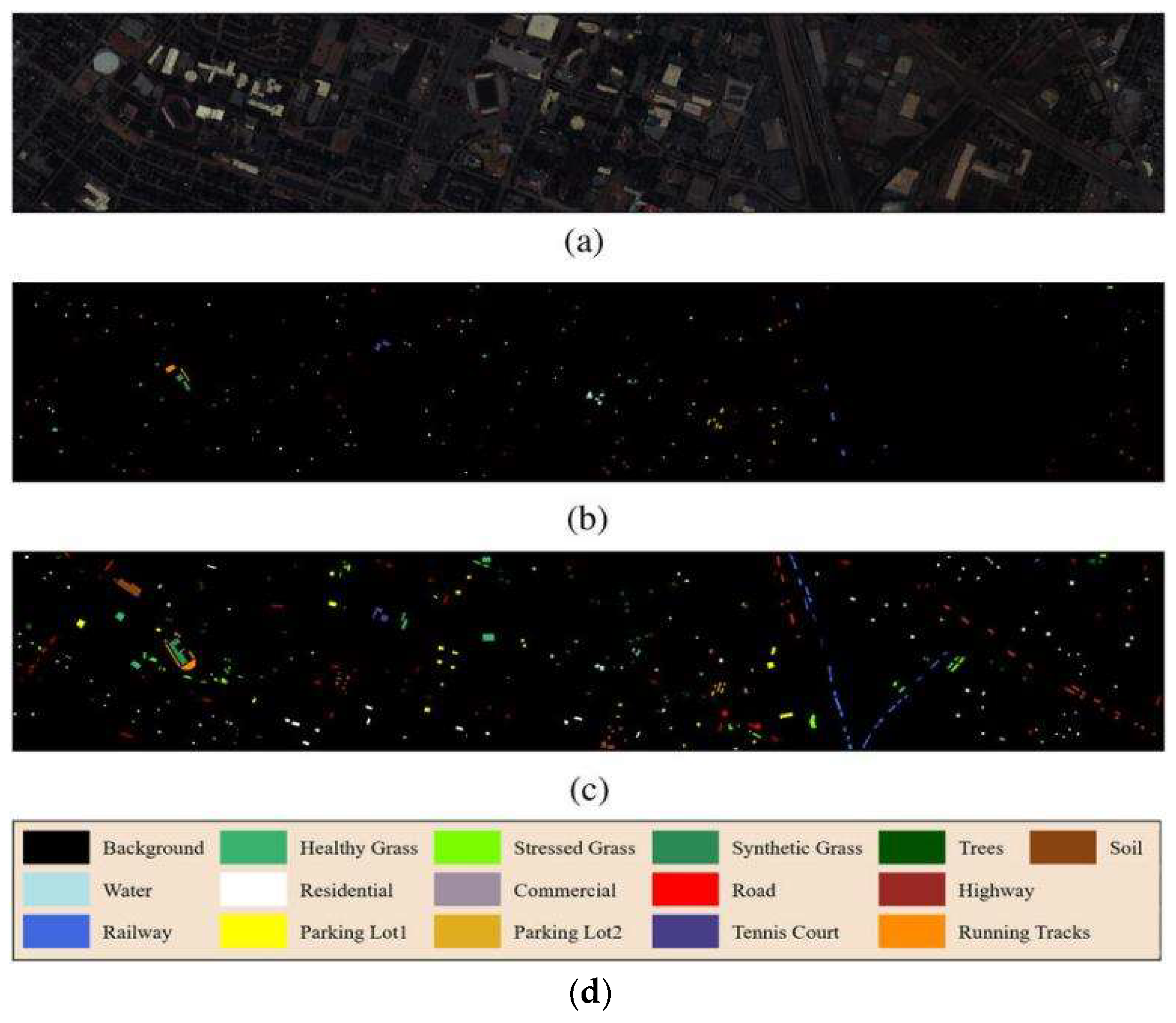
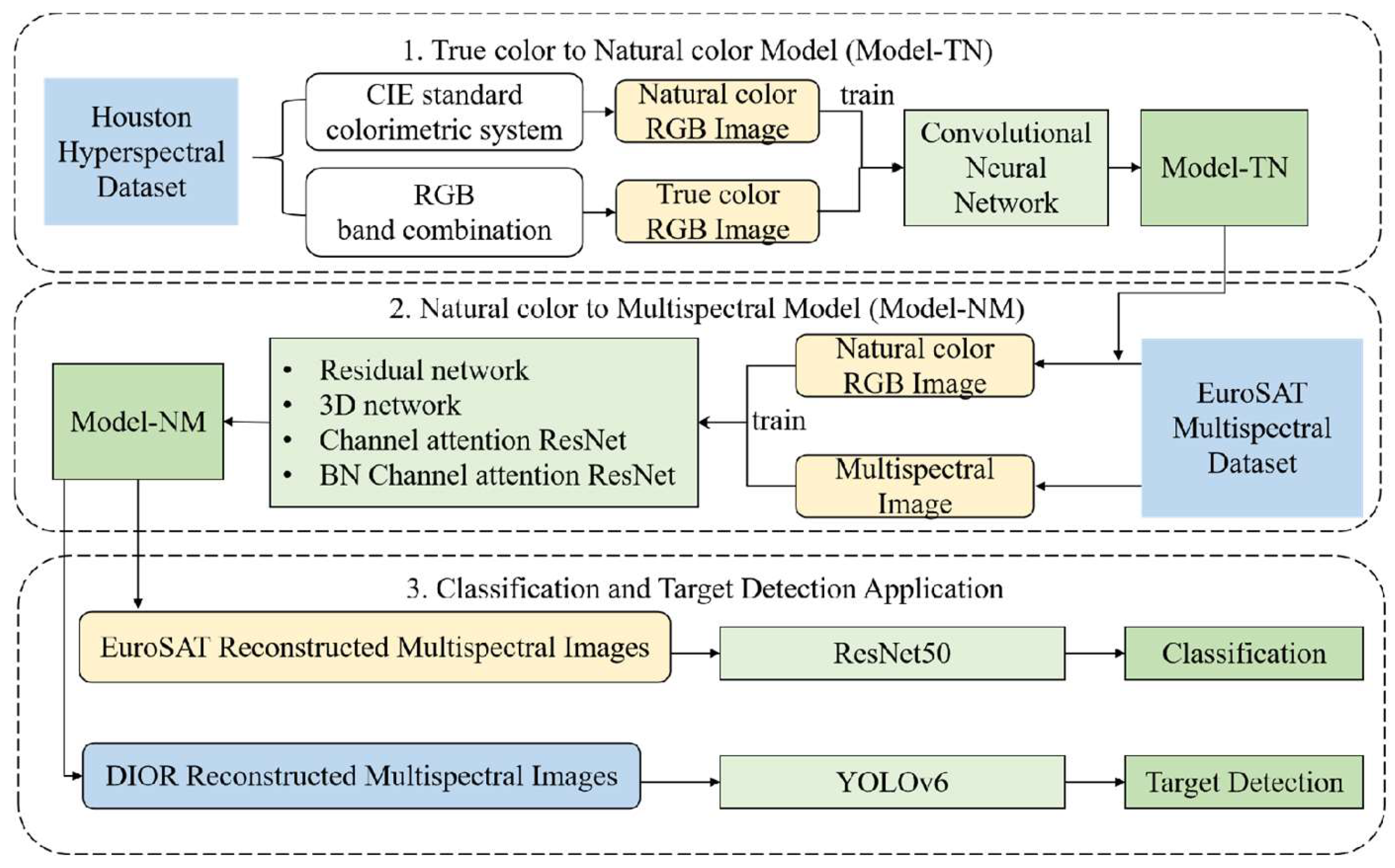
The flowchart of the multispectral image reconstruction algorithm and subsequent applications is shown in Figure 4. This paper first addresses the issue of lacking insufficient paired multispectral and natural color images by combining the design of a novel deep learning model (i.e., Model-TN) based on the Houston hyperspectral dataset, and standard colorimetric systems theory. Then, we propose a multispectral reconstruction model (i.e., Model-NM) using the residual network integrated with channel attention mechanisms for the reconstruction of multispectral images. Finally, the effectiveness of the Model-NM is further verified, by applying the reconstructed multispectral images to image classification and object detection. Relevant methods are introduced in detail as follows.

2.2.1. True to Natural Color RGB Method Model-TN

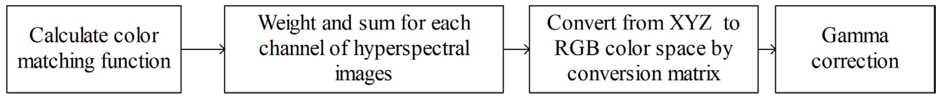
Firstly, the ncRGB images corresponding to the hyperspectral images were generated using the Houston hyperspectral image dataset and the CIE tristimulus curves. The tristimulus curves of the CIE standard colorimetric system theory, also known as the CIE color matching function (CMF), can convert images to the corresponding CIE color space [25,26,27,28,29]. Additionally, the hyperspectral image reflectance at different wavelengths and the spectral power distribution of the corresponding light source were also used, by which the ncRGB images were generated from the hyperspectral reflectance images. The specific operation process is shown in Figure 5.

$$X={\displaystyle \frac{K}{N}}{\int }_0^{\infty }S\left(\lambda \right)I\left(\lambda \right)\overline{x}\left(\lambda \right)d\lambda$$

(1)

$$Y={\displaystyle \frac{K}{N}}{\int }_0^{\infty }S\left(\lambda \right)I\left(\lambda \right)\overline{y}\left(\lambda \right)d\lambda$$

(2)

$$Z={\displaystyle \frac{K}{N}}{\int }_0^{\infty }S\left(\lambda \right)I\left(\lambda \right)\overline{z}\left(\lambda \right)d\lambda$$

(3)

$$N={\int }_0^{\infty }I\left(\lambda \right)\overline{y}\left(\lambda \right)d\lambda$$

(4)

where X, Y, and Z are the response values of the CIE XYZ color space, as a function of wavelength λ, object reflectance S(λ), the spectral power distribution of the light source I(λ), three-stimulus curves N, and proportionality factor K. $\overline{x}\left(\lambda \right)$, $\overline{y}\left(\mathsf{\lambda }\right)$, and $\overline{z}\left(\lambda \right)$ are tristimulus values. The parameter N can normalize the response values, and K serves as a proportionality factor, typically set to 100. After obtaining X, Y, and Z through weighted summation, the corresponding conversion matrix is selected based on the color spaces before and after conversion and the light source, as shown in

Table 2. Information of color space transformation matrix.

RGB Working Space	Reference White	RGB to XYZ	XYZ to RGB
sRGB	D65	M	M−1

. Then, X, Y, and Z are converted to the corresponding color space using the conversion matrix, as illustrated in (5), and the numerical values of M and M⁻¹ are given as (6) and (7), respectively.

$$\left[\begin{array}{c}{R}_{lin}\\ G_{lin}\\ B_{lin}\end{array}\right]=M\left[\begin{array}{c}X\\ Y\\ Z\end{array}\right]$$

(5)

$$M=\left[\begin{array}{ccc}0.4124564& 0.3575761& 0.1804375\\ 0.2126729& 0.7151522& 0.0721750\\ 0.0193339& 0.1191920& 0.9503041\end{array}\right]$$

(6)

$$M^{-1}=\left[\begin{array}{ccc}3.2404542& -1.5371385& -0.4985314\\ -0.9692660& 1.8760108& 0.0415560\\ 0.0556434& -0.2040259& 1.0572252\end{array}\right]$$

(7)

Finally, a Gamma correction converted the response values (ranging from 0 to 1) to the RGB color space using a segmented nonlinear function, such as the one represented in (8), for correction. In simpler cases, Formula (9) can be used instead. Then, the R, G, and B values are clipped to [0, 1] and stored as 8bit integers (0–255) to be correctly displayed on the screen.

$$C=\left\{\begin{array}{c}12.92C_{lin },C_{lin}\le 0.0031308\\ 1.055C_{lin}^{{\displaystyle \frac{1}{2.4}}}-0.055,C_{lin}\ge 0.0031308\end{array}\right.$$

(8)

$$C=C_{lin}^{{\displaystyle \frac{1}{\gamma }}},\hspace{0.33em}\gamma =2.2$$

(9)

In this paper, the CIE 1964 XYZ CMF was selected, where the spectral power distribution of the standard daylight source D65 was utilized. The Houston hyperspectral images were employed to generate the corresponding ncRGB images. Because the spectrum of the hyperspectral image is not continuous, appropriate CMF values were selected based on the wavelength of each hyperspectral image channel. The CMF wavelengths range from 400 nm to 700 nm, with an interval of 10 nm. For each channel, the wavelength closest to that of the CMF was chosen from the hyperspectral image. Since the wavelengths of the hyperspectral image channels are discontinuous, the rectangular method was used to solve the integral as shown in Formulas (10)–(13):

$$X={\displaystyle \frac{K}{N}}\sum _{i=1}^{30}S\left(400+10i\right)I\left(400+10i\right)\overline{x}\left(400+10i\right)d$$

(10)

$$Y={\displaystyle \frac{K}{N}}\sum _{i=1}^{30}S\left(400+10i\right)I\left(400+10i\right)\overline{y}\left(400+10i\right)d$$

(11)

$$Z={\displaystyle \frac{K}{N}}\sum _{i=1}^{30}S\left(400+10i\right)I\left(400+10i\right)\overline{z}\left(400+10i\right)d$$

(12)

$$N=\sum _{i=1}^{30}I\left(400+10i\right)\overline{y}\left(400+10i\right)d$$

(13)

where $d$ is the interval of the wavelength of the CMF ($d$ = 10), and the other parameters have the same physical meaning as the parameters of the Formulas (1)–(4).

First, normalize the hyperspectral data to [0, 1] according to the data storage format of Houston Hyperspectral Dataset. After converting hyperspectral image data into XYZ color space values, the conversion matrix is transformed from XYZ to sRGB color space. Then, a gamma correction was applied to make the image more consistent with human vision to obtain an ncRGB image. After applying the transfer function and gamma correction, the R, G, and B values are clipped to [0, 1] and stored as 8bit integers (0–255).

Finally, ncRGB images and tcRGB images generated from the Houston hyperspectral dataset as float32 tensors in the 0–1 range were employed to train the Model-TN for converting tcRGB images into ncRGB images. The CNN was employed to train Model-TN, and the model structure employed during training is illustrated in Figure 6. The first convolutional layer performs preliminary feature extraction from the 3-channel image data, converting it into 64-channel feature maps. Next, a convolution activation layer further extracts feature information while maintaining the channel number of the feature map. Finally, a convolutional layer can transform the 64-channel feature map into a 3-channel ncRGB image.

Houston true and natural color image pairs were trimmed to a same size of 64 × 64 pixels for model training and validation. Two-thirds of the images were allocated to the training set, while one-third were reserved for the verification set. The experiments were conducted using Python 3.9, with the deep learning framework based on Pytorch 2.3. The hardware configuration includes an Intel Core i5-13490F processor (Intel Corporation, Santa Clara, CA, USA, sourced from China), an NVIDIA GeForce RTX 4060 Ti GPU (PC Partner, Singapore, sourced from China), and a 32 GB CPU memory. The loss function used the mean relative absolute error (MRAE), where the batch size was set to 1. We selected the Adamax optimizeris, and the learning rate was set to 0.001 to avoid a divisor of zero. The learning rate was multiplied by 0.98 every 200 epochs until the loss function stopped decreasing over a span of 200 epochs. To obtain the best training model parameter of the Model-TN, we select the MRAE as the loss. Meanwhile, the MRAE and Root Mean Square Error (RMSE) are used to evaluate the accuracy of the Model-TN, which are defined as follows:

$$MRAE={\displaystyle \frac{1}{n}}\sum _{i=1}^n\left({\left(\right|I}_{gt}^{\left(i\right)}-I_{re}^{\left(i\right)}\left|\right)/I_{gt}^{\left(i\right)}\right)$$

(14)

$$RMSE=\sqrt{{\displaystyle \frac{1}{n}}\sum _{i=1}^n({I_{gt}^{\left(i\right)}-I_{re}^{\left(i\right)})}^2}$$

(15)

where $n$ represents the number of image pixels, and $I_{gt}^{\left(i\right)}$ and ${ I}_{re}^{\left(i\right)}$ refer to the pixel value of the ground truth and the reconstructed result, respectively.

2.2.2. Multispectral Reconstruction Method Model-NM

Considering the high-performance of the deep learning method, the residual network was selected as the basic method of the multispectral image reconstruction model-NM. The gradient of the backpropagation of the residual network [30] consists of two parts, the identity mapping of x with the gradient of 1 and the gradient of multilayer traditional neural network mapping. When a specific layer in the network converges to an optimal state, the local gradient vanishes, inhibiting backpropagation of the error signal to earlier layers. Consequently, parameters that should remain stable continue to be updated, potentially increasing the overall model error. Particularly, we incorporated a shortcut connection, which can allow the gradient value to remain at 1 when the optimal solution for a layer is reached. This allows deeper gradients to be effectively transferred to the shallower layers, enabling the weight parameters of the shallow-layer network to be effectively trained and avoiding the problem of gradient disappearance.

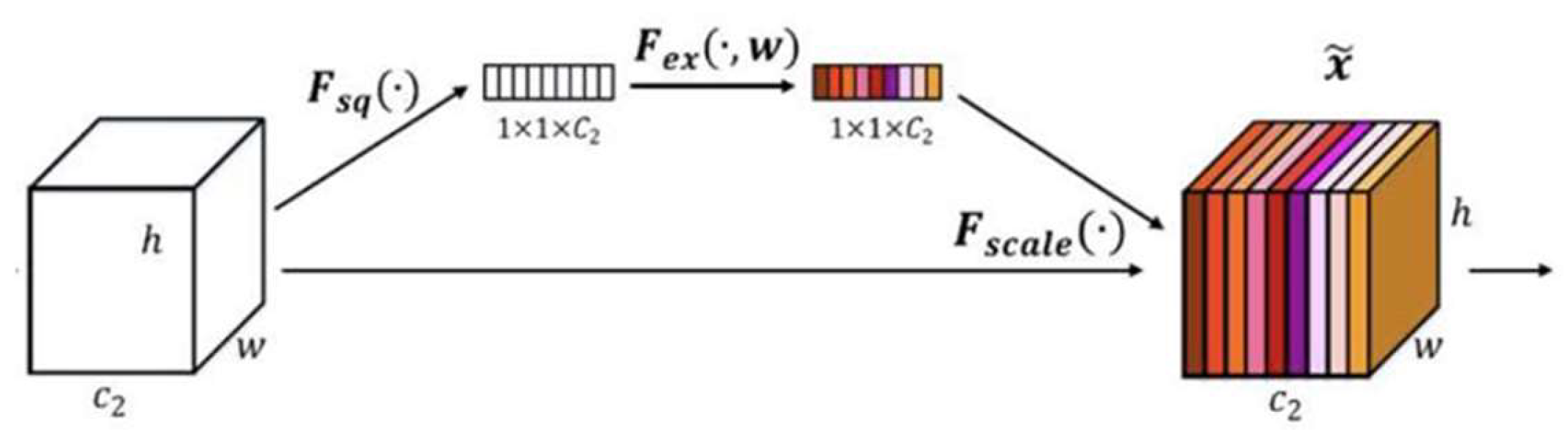
Based on the residual network model, the channel attention mechanism using Squeeze-and-Excitation (SE) block is innovatively added to enhance the focus on the differences between channels during model training, which consists of two primary steps as shown in Figure 7. The first step is compression. The pooling of the feature map with a size of h × w × c can result in the information of each channel being compressed into a single value, thereby generating a global compressed feature with a size of 1 × 1 × c. The second step is excitation. The global compressed features obtained from the first step were further processed through a structure consisting of a fully connected layer, another fully connected layer (i.e., the ReLU activation layer), and a Sigmoid layer. This process yields the weights for each channel in the feature map, which were then used to weight the original feature map, resulting in a processed feature map. The first fully connected layer compresses c channels into c/r channels to reduce the computational load, and then the second fully connected layer restores the number of channels to c channels through a ReLU nonlinear activation layer. Finally, the normalized weights were obtained by activating the Sigmoid function. r is the ratio of compression, and it is not possible to use both the ReLU nonlinear activation function and the Sigmoid function if only one fully connected layer is used.

Figure 8 shows the overall structure of the channel attention residual network model, Model-NM, proposed in this paper. The input data is an image as float32 tensors in the 0–1 range with a height of 64 pixels, a width of 64 pixels, and 3 channels for RGB (red, green, and blue). The reconstructed multispectral images contain five bands. So, the output data is an image with a height of 64 pixels, a width of 64 pixels, and 5 channels for blue, green, red, red edge, and near-infrared. These five bands and their wavelengths respectively correspond to b02, b03, b04, b05, and b08 in the EuroSAT dataset as listed in Table 1.

The specific operation process is as follows. The network first processes the 64 × 64 × 3 RGB input through an initial 3 × 3 convolution (3 to 64 channels) with a ReLU activation. The feature map then passes through three consecutive residual blocks, where each block contains the following parts: (1) two 3 × 3 convolutional layers (64 to 64 channels) with a ReLU activation; (2) an identity skip connection; and (3) element-wise addition followed by a ReLU.

Critically, after the residual blocks but before the SE module, the network applies an intermediate 3 × 3 convolutional layer (64 to 64 channels) with a ReLU activation to further refine feature representations.

The processed features then enter the Squeeze-and-Excitation (SE) module (compression ratio r = 16), which dynamically recalibrates channel weights through the following processes: (1) global average pooling to generate channel-wise statistics; (2) two fully connected layers (64 to 4 to 64) with ReLU and Sigmoid activation, respectively; and (3) channel-wise multiplication with the input feature map. Finally, a 3 × 3 convolution projects the 64-channel features to 5 output bands (B02/B03/B04/B05/B08), preserving the 64 × 64 spatial resolution throughout the network via symmetric padding.

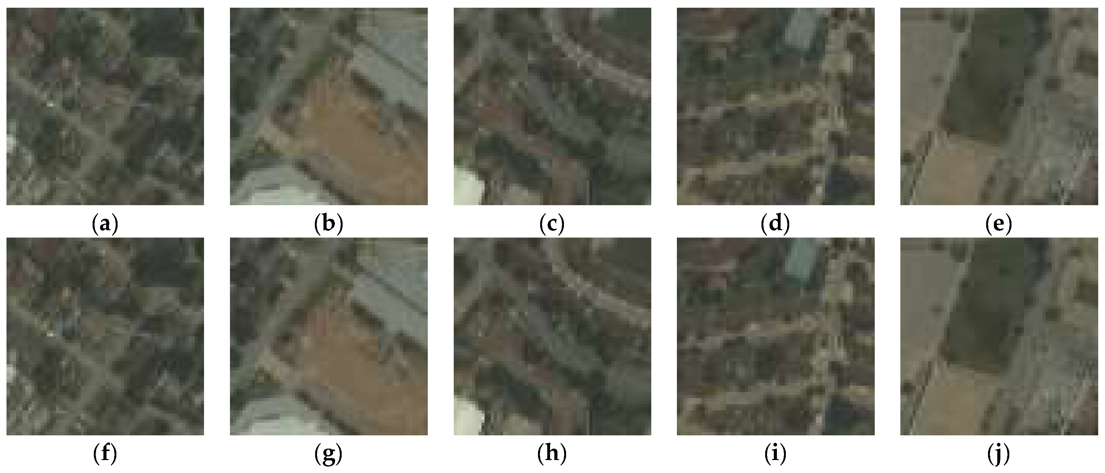
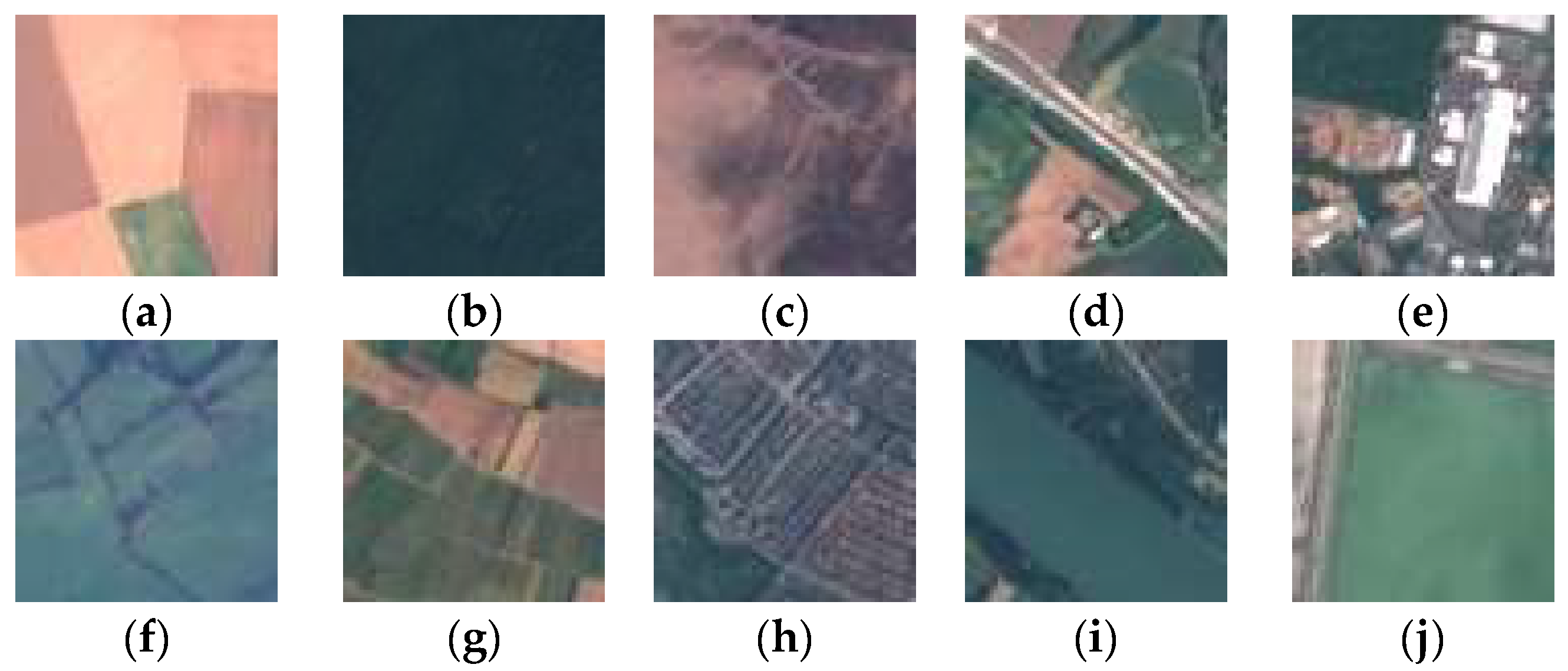
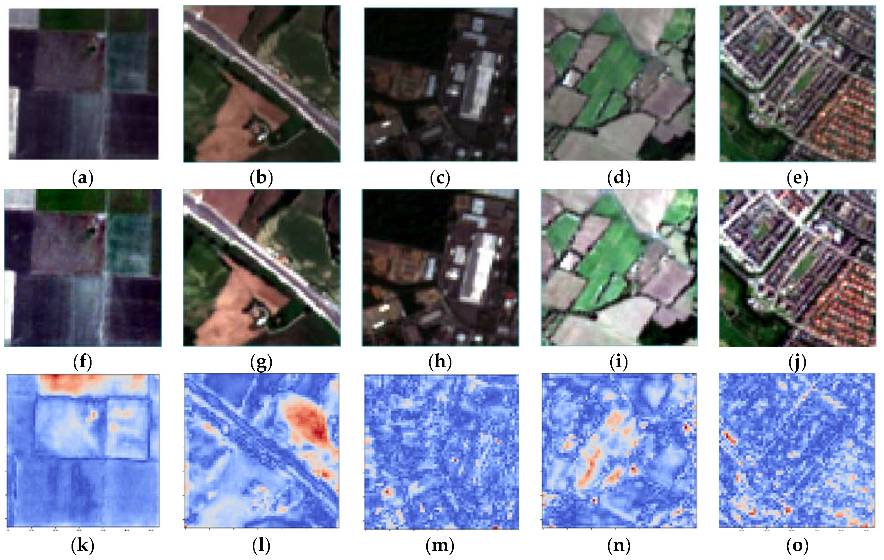
EuroSAT multispectral images in five bands mentioned above and corresponding ncRGB images generated through the Model-TN introduced in Section 3.1 were collected as training image paeqirs. Data for categories 1–7 and 9 (N = 21,000 images) (see Figure 2a–g,i) were used for training, where 2/3 of data were composed of training sets while 1/3 of the total were used as validation sets. Additionally, image pairs for the other two categories (i.e., Figure 2h,j) were used to test the accuracy and generalization ability of the Model-NM.

The programming language Python 3.9 was employed, with the deep learning framework based on PyTorch 2.3. The hardware configurations include an Intel Core i5-13490F processor (Intel Corporation, US CA Santa Clara, sourced from China), an NVIDIA GeForce RTX 4060 Ti GPU (PC Partner, Singapore, sourced from China), and 32 GB of CPU memory. The loss function employed is the MRAE, and the batch size was set to 16. The optimizer used was Adamax, with a learning rate of 0.001. The exponential decay rates were set to 0.9 and 0.999 to prevent the denominator from approaching zero. The learning rate was multiplied by 0.98 every 200 epochs until the loss function ceased to decrease over a span of 200 epochs.

Similarly to the training process of the Model-TN, we also select MRAE as the loss to train the Model-NM. In addition, the MRAE, RMSE, and Spectral Information Divergence (SID) are employed to evaluate the accuracy of the Model-NM with a formula as follows:

$$SID={\displaystyle \frac{1}{n}}\sum _{i=1}^n\left({\displaystyle \frac{I_{gt}^{\left(i\right)}}{\left|I_{gt}^{\left(i\right)}\right|}}-{\displaystyle \frac{I_{re}^{\left(i\right)}}{\left|I_{re}^{\left(i\right)}\right|}}\right)\left(\log \left({\displaystyle \frac{I_{gt}^{\left(i\right)}}{\left|I_{gt}^{\left(i\right)}\right|}}\right)-\log \left({\displaystyle \frac{I_{re}^{\left(i\right)}}{\left|I_{re}^{\left(i\right)}\right|}}\right)\right)$$

(16)

where $n$, $I_{gt}^{\left(i\right)}$, and $I_{re}^{\left(i\right)}$ refer to the same meaning as formulas (14) and (15).

2.2.3. Image Classification Method

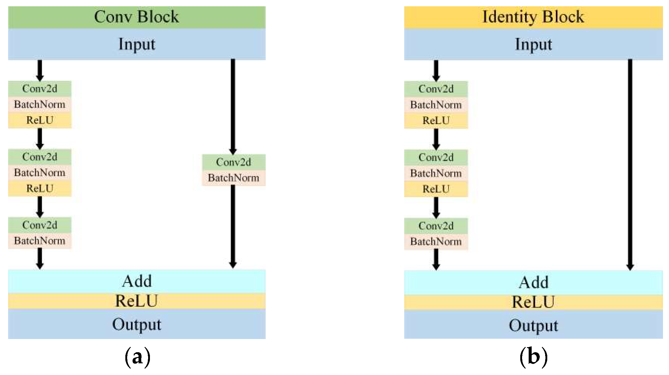
The classical network model ResNet50 was employed for image classification, which consists of two fundamental blocks including the Conv Block and the Identity Block as illustrated in Figure 9. The Conv Block alters the input and output dimensions to prepare for the subsequent use in the Identity Block. It should be noted that the Conv Blocks cannot be used in series. In contrast, the Identity Block maintains the same input and output dimensions and can be used in series, which allows for a deeper network and the extraction of more complex features.

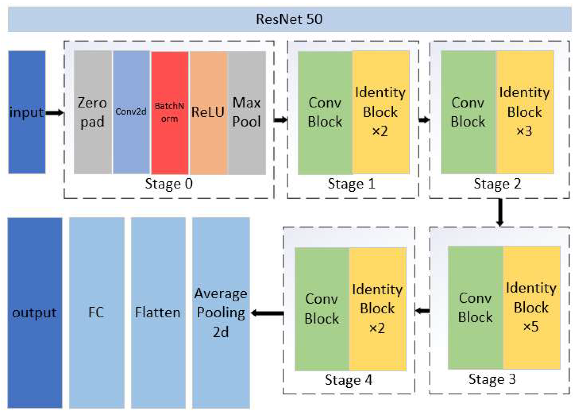
Figure 10 illustrates the main structure of ResNet50, which consists of five stages. Stage 0 serves as the preprocessing stage, where the data are adjusted into suitable forms for training and initial feature extraction from the images. Stages 1–4 share a similar structure and function, where a Conv Block is followed by several Identity blocks. Specifically, Stages 1–4 connect Identity blocks 2, 3, 5, and 2 after the Conv Block, respectively. This design aims to deepen the network and enhance the extraction of deep features from the images. Finally, the extracted information is pooled and fully connected to classify the images. The CNN was also used to train the image classification model, which can reduce memory usage in the deep network. By using three key operations including local receptive fields, weight sharing, and pooling layers, it can effectively decrease the number of network parameters and help mitigate the overfitting problem of the model.

Based on the ResNet50 model, this paper modified stage 0 to adjust the height, width, and channel size of the input images. This adjustment allows the model to adapt to the multispectral images of the EuroSAT dataset, the generated ncRGB image, and the reconstructed multispectral image.

Categorical cross entropy (i.e., Equation (17)) was used as the Loss function for training the classification model, where $C$ represents the number of target object classes and $N$ is the number of samples. $y_{i,j}$ represents the true value of the sample $i$ belonging to the $j$ class. If the sample $i$ belongs to the $j$ class, then ${ y}_{i,j}=1$, otherwise ${ y}_{i,j}=$0. $P_{i,j}$ represents the probability of predicting the sample $i$ to be class $j$.

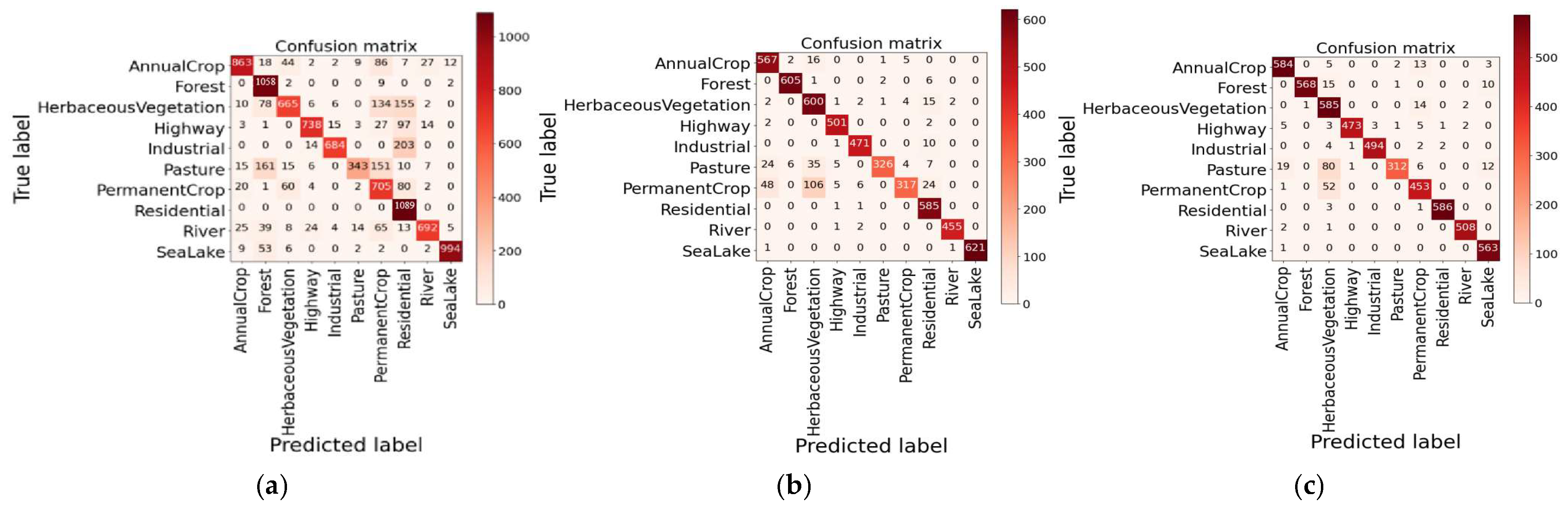
The precision, recall, and overall accuracy are selected to evaluate classification accuracy as shown in Formulas (18)–(21), which are defined based on the confusion matrix given in Equation (22). $n_{ij}$ represents the number of samples of Class $i$ predicted to be Class $j$. $\sum _{j=1}^C{n}_{ij}$ represents the total number of Class $i$ samples, and $\sum _{i=1}^C{n}_{ij}$ refers to the total number of samples predicted as Class $j$.

$$Loss=-{\displaystyle \frac{1}{N}}{\sum }_{i=1}^N{\sum }_{j=1}^C{y}_{i,j}\mathit{log}\left(P_{i,j}\right)$$

(17)

$$Precision={\displaystyle \frac{n_{jj}}{\sum _{i=1}^C{n}_{ij}}}$$

(18)

$$Recall={\displaystyle \frac{n_{ii}}{\sum _{j=1}^C{n}_{ij}}}$$

(19)

$$Overall Accuracy={\displaystyle \frac{\sum _{i=1}^C{n}_{ii}}{\sum _{i=1}^C\sum _{j=1}^C{n}_{ij}}}$$

(20)

$$F_1=2\times {\displaystyle \frac{Precision\times Recall}{Precision+Recall}}$$

(21)

$$\left[\begin{array}{cccc}{n}_{11}& n_{12}& \dots & n_{1c}\\ n_{21}& n_{22}& \dots & n_{2c}\\ \dots & \dots & \dots & \dots \\ n_{c1}& n_{c2}& \dots & n_{cc}\end{array}\right]$$

(22)

2.2.4. Target Detection Method

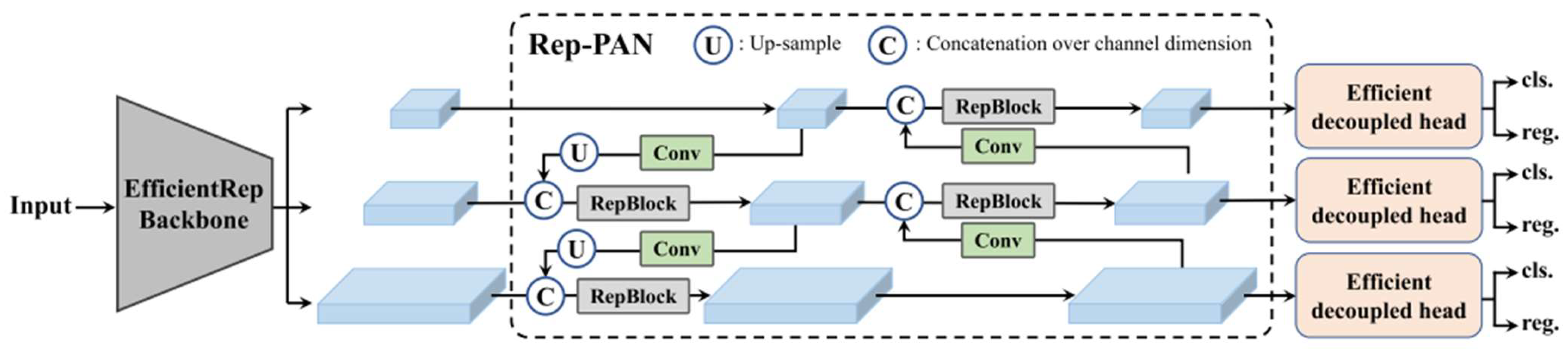
The target detection method employs the YOLOv6 algorithm [31], which consists of three main components: the backbone network, the neck, and the head, as shown in Figure 11. The backbone network primarily determines the model’s feature representation capability. The neck aggregates low-level physical features with high-level semantic features and constructs pyramidal feature mappings across all levels. The head comprises multiple convolutional layers that predict the final detection results based on the multi-level features assembled by the neck. In the YOLOv6 algorithm, these components are referred to as EfficientRep, EfficientRep-PAN, and Efficient Decoupled Head, respectively.

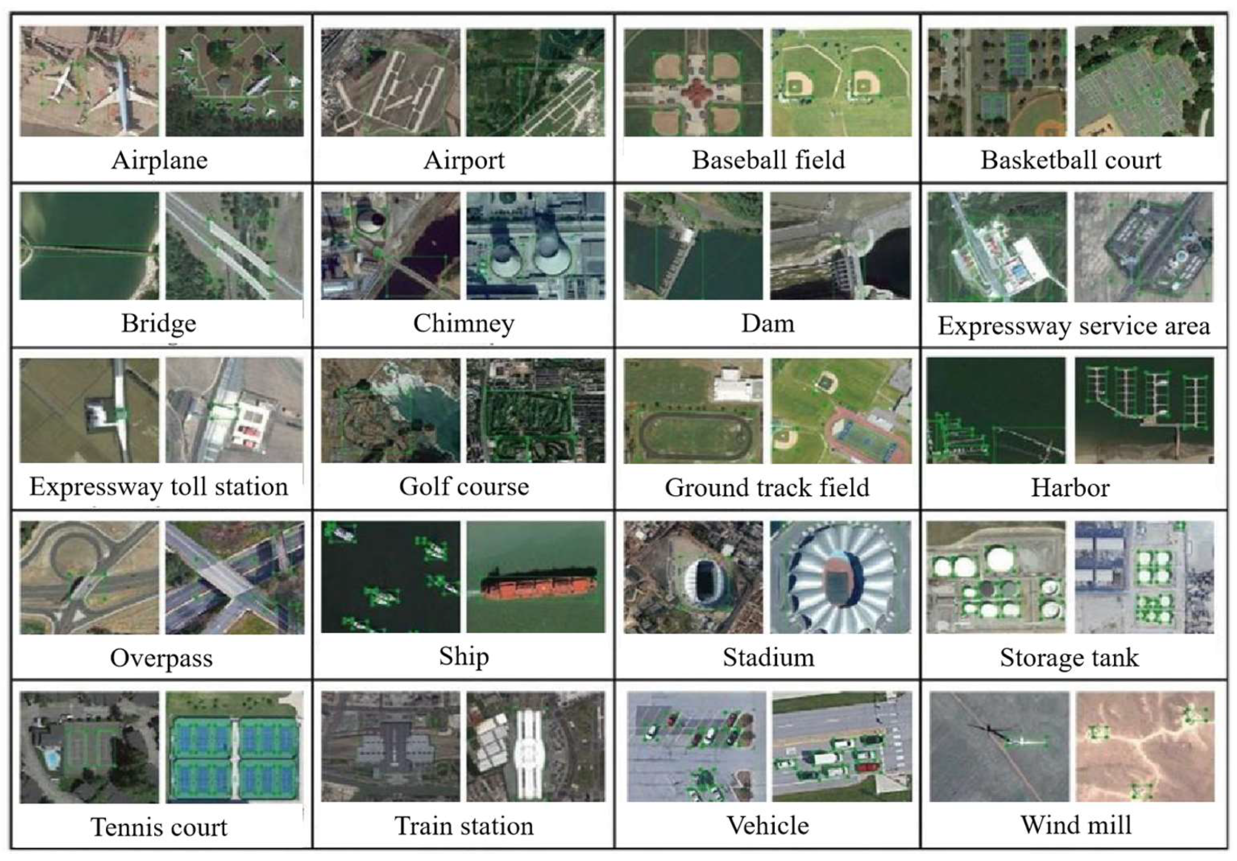
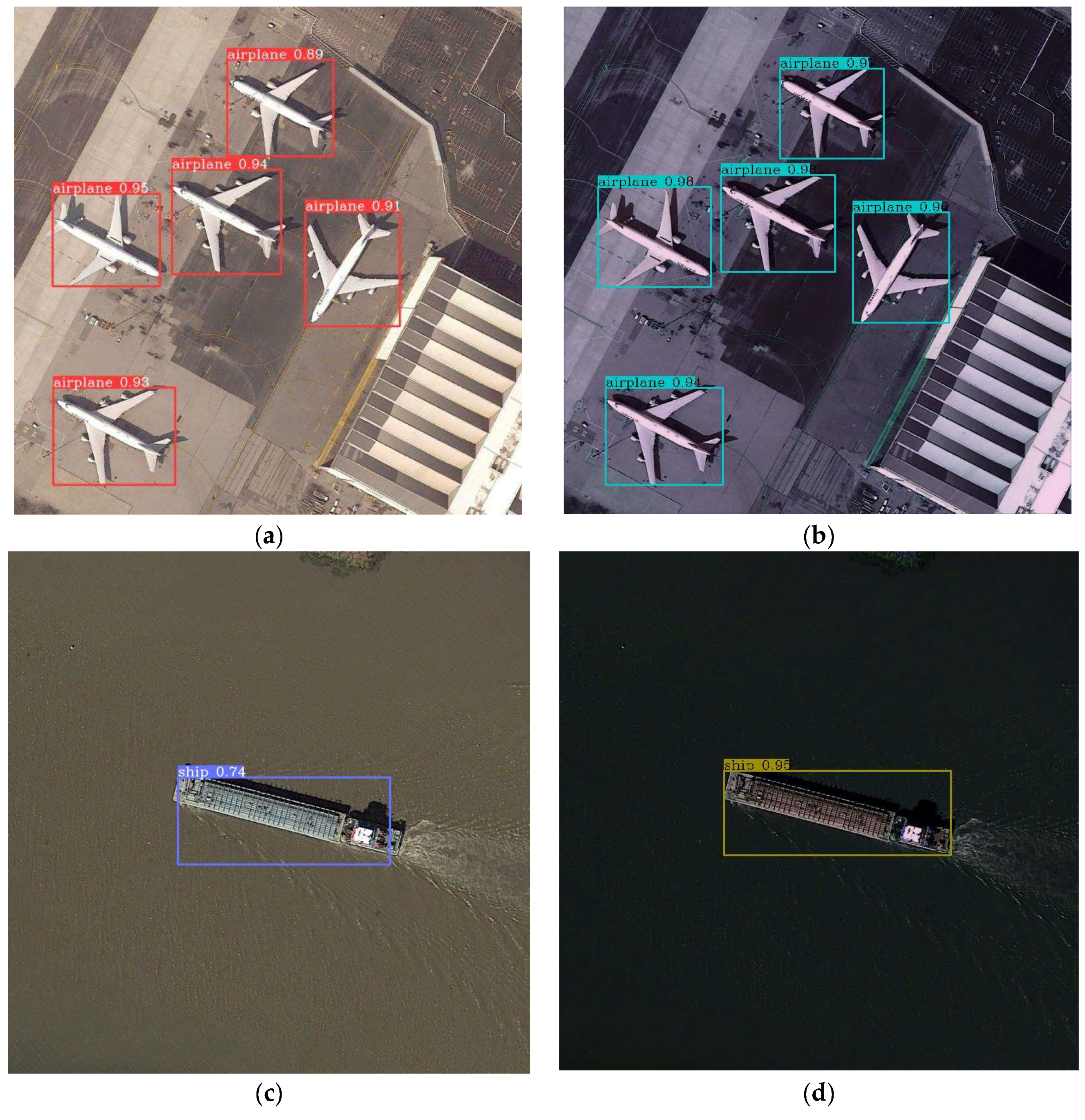
The RGB image of the DIOR dataset was applied to the multispectral image reconstruction model, Model-NM, to generate the reconstructed multispectral image of the DIOR dataset. In this paper, based on YOLOv6 algorithm, the reconstructed multispectral image of the DIOR dataset and the original RGB image were, respectively, identified, and the differences in target recognition results were compared. The input layer of the model was changed from 3 layers to 5 layers when the object detection of the reconstructed multispectral image was carried out.

The Intersection over Union (IoU) loss (i.e., ${\mathrm{L}\mathrm{o}\mathrm{s}\mathrm{s}}_{\mathrm{I}\mathrm{o}\mathrm{U}}$) and Classification Binary Cross Entropy Loss (i.e., ${Loss}_{cls}$) were selected to train the target detection model, and we used average precision (i.e., AP) and mean AP (i.e., mAP) to evaluate target detection accuracy. The number of batches was set to 20. Their Formulas (23)–(26) are as follows.

$${Loss}_{IoU}=1-IoU+{\displaystyle \frac{d^2}{c^2}}+av$$

(23)

$${Loss}_{cls}=-{\displaystyle \frac{1}{N}}\sum _{i=1}^N\left(y_i\mathit{log}\left(P_i\right)+\left(1-y_i\right)\mathit{log}\left({1-P}_i\right)\right)$$

(24)

$$AP=\sum _i^{n-1}\left(r_{i+1}-r_i\right)P\left(r_{i+1}\right)$$

(25)

$$mAP={\displaystyle \frac{1}{C}}\sum _{i=1}^C{AP}_i$$

(26)

In Equation (23), $IoU$ represents the ratio of the overlapping area to the total area between the ground truth box and the predicted box. $d$ refers to the Euclidean distance between the center points of the ground truth box and the predicted box, and $c$ is the diagonal distance of the smallest enclosing box that fully contains both the ground truth and predicted boxes. $v$ represents the aspect ratio between the ground truth box and the predicted box, and $a$ is the weight balancing parameter. In Equation (24), $N$ represents the number of samples, and ${ y}_i$ and $P_i$ are the round truth labels and the model predictions, respectively.

In Equations (25) and (26), $n$ represents the number of horizontal ordinate points on the precision recall curve after interpolation. $r_i$ represents the recall value corresponding to the horizontal ordinate points in ascending order, and $\mathrm{P}$ represents precision corresponding to the $r_n$. mAP at the $IoU$ of 0.5 (hereafter mAP(0.5)) is used, as well as the average value of mAP at the $IoU$ ranging from 0.5 to 0.95 with a step of 0.05 (hereafter mAP(0.5–0.95)).

The experiment used Python 3.9 for programming, with the deep learning framework based on PyTorch 2.4. The hardware consists of an Intel Core i5-10200H processor (Intel Corporation, Santa Clara, CA, USA, sourced from China), an NVIDIA GeForce GTX 1650 GPU (NVIDIA, Santa Clara, CA, USA, sourced from China), and 16 GB of CPU memory.

3. Results

3.1. Accuracy Analysis of True-to-Natural Method Model-TN

The tcRGB image of the Houston hyperspectral image is shown in Figure 12a, while the ncRGB image generated by the CIE standard chromaticity system is presented in Figure 12b. It can be seen that the tcRGB image is more saturated with higher contrast, displaying a larger difference between black and white. In contrast, the ncRGB image appears more natural and aligns more closely with RGB images taken under real lighting conditions. The Model-TN training accuracies are shown in

Table 3. Training accuracy of neural network models.

Evaluation Metric
MRAE	0.0081
RMSE	0.0033

. The MRAE is 0.0081 and less than 0.01, which meets the requirements.

The comparison between the ncRGB image generated by the model and that generated by the CIE standard chromaticity system is shown in Figure 13. To show the difference between these two results intuitively, the RMSE errors plot of each pixel between these two methods is also shown in the range of 0–255 with cold and warm colors. The closer it is to 0, it will appear to be blue, while it will appear to be red when the RMSE is close to 255.

It is difficult for the naked eye to discern the differences between the ncRGB images generated by the two methods. Their error plots predominantly display blue, indicating a low contrast. The small error values for similar types of objects indicate consistent ncRGB values for these two methods, while only some distinct types of objects exhibit inconsistent color shades. This suggests that the errors in the ncRGB images produced by both methods are minimal, and the proposed Model-TN method shows robust applicability across various object categories to generate ncRGB data from easily available multispectral images, such as free available satellite global observations.

3.2. Multispectral Reconstruction Model-NM Accuracy Evaluation Using the EuroSAT Dataset

The EuroSAT dataset was used to train the Model-NM for multispectral image reconstruction from ncRGB data. The convergence process of the MRAE during training is illustrated in Figure 14. It consistently decreases from epoch 0 to 1000, converging to approximately 0.0420 between 1000 and 1400 epochs. Then, training halts after 200 epochs when the minimum verification loss no longer decreases.

Table 4. Validation accuracies of channel attention residual network.

Evaluation Metric
MRAE	0.0420
RMSE	0.0175
SID	0.0121

presents the verification accuracies of the network model on the verification set, which meets the requirements.

After training, the test accuracies of Model-NM are reported in

Table 5. Test accuracies of channel attention residual network.

Class	Evaluation Metric
	MRAE in Five Bands	RGB MRAE	RED EDGE MRAE	NIR MRAE	RMSE	SID
Annual Crop	0.03034	0.0072	0.0547	0.0755	0.0162	0.0062
Forest	0.04312	0.0100	0.0753	0.1104	0.0179	0.0088
Herbaceous Vegetation	0.03251	0.0078	0.0578	0.0813	0.0118	0.0061
Highway	0.0432	0.0091	0.0726	0.1161	0.0183	0.0117
Industrial	0.0411	0.0103	0.0648	0.1098	0.01534	0.0104
Pasture	0.0364	0.0086	0.0633	0.0931	0.0190	0.0067
Permanent Crop	0.0324	0.0076	0.0563	0.0829	0.0150	0.0063
Residential	0.0436	0.0113	0.0636	0.1206	0.0163	0.0113
River	0.0609	0.0092	0.1099	0.1673	0.0209	0.0259
Sea Lake	0.5925	0.0188	1.1213	1.7846	0.0380	0.3666
All (classes 1–7 and 9)	0.0397	0.0087	0.0690	0.1037	0.0166	0.0101

. Reconstruction errors (MRAE, RMSE, and SID) are listed per class for all ten EuroSAT categories and per spectral group (all five bands, RGB bands, red edge, and NIR). Note that the final “All (classes 1–7 and 9)” row in Table 5 aggregates only the eight classes used for training; classes 8 and 10 were held out for testing. An overall MRAE of 0.0397 is obtained for channel attention ResNet proposed in this study, which meets the general accuracy requirement. Among 10 object categories, small MRAEs less than 0.044 can be seen for training categories 1–7. Meanwhile, a similarly high accuracy was observed for the algorithm transfer to “Residential”, which demonstrates the model generalization. However, when the Model-NM trained by the category “River” is used for “Sea Lake”, large errors are obtained including MRAE, RMSE, and SID, which indicates the Model-NM still meets challenges over water areas. In terms of bands, it shows a high accuracy for reconstructing multispectral image in RGB bands, which can be understood because of wavelength similarities with ncRGB data. Notably, relatively larger MRAEs are seen in red edge and NIR bands due to significant wavelength differences with ncRGB data.

The reconstructed multispectral images were compared with the original multispectral image, displayed as the tcRGB image as shown in Figure 15. To illustrate the differences between these two kinds of images more intuitively, the RMSE of each pixel was normalized and mapped to a range of 0–255, with colors corresponding to warm and cool tones. Values closer to 0 are filled in blue, while those closer to 255 are displayed in red. The error diagram clearly highlights the differences in multispectral image reconstruction for various types of objects.

As shown in the comparison charts (i.e., Figure 15k–o), there are small overall differences between the original and reconstructed multispectral images without obvious discrepancies. The error charts illustrate that the overall color is blue, indicating a small level of error. However, the error in certain regions is larger than those in other data, suggesting that the effectiveness of the Model-NM for multispectral reconstruction varies for different types of objects.

Meanwhile, we compare the test results of several different network models.

Table 6. Test accuracies of different networks.

Methods	Evaluation Metric
	MRAE	RMSE	SID
ResNet50 (2D residual)	0.0445	0.0191	0.0155
3D CNN	0.0451	0.0194	0.0157
SE ResNet	0.0397	0.0166	0.0101
BN SE ResNet	0.0403	0.0170	0.0104

compares four network backbones: ResNet50 (2D residual), a 3D CNN, a Squeeze-and-Excitation ResNet (SE ResNet), and the same with batch normalization (BN SE ResNet) on the EuroSAT test set (classes 1–7 and 9, N = 7000 images). All models were trained under identical hyperparameters (batch size = 16, Adamax optimizer, initial LR = 0.001 with 0.98 decay every 200 epochs) and evaluated with three metrics: MRAE, RMSE and SID, as referred to in Section 2.2.2. Compared with ResNet, 3D CNN, and BN SE ResNet, the MRAE of channel attention residual network reconstruction is the lowest, which is 0.0397. In terms of the other two indicators, RMSE and SID, the channel attention residual network also shows optimal accuracy, which demonstrates the high accuracy of the Model-NM using a channel attention residual network proposed in this study.

3.3. Image Classification Application Using the EuroSAT Dataset

The Model-NM is applied to image classification to further evaluate model effectiveness based on the EuroSAT dataset. First, ncRGB images generated by the Model-TN were employed for classification application, which comprise a total of 27,000 images for 10 categories. The confusion matrix for ncRGB image classification is shown in Figure 16a. Overall accuracy, precision, and recall for classification test experiments are detailed in

Table 7. Image classification test accuracies over different land types in EuroSAT dataset.

Class	ncRGB Image			Original Multispectral Image					Reconstructed Multispectral Image
	Precision	Recall	F1	Precision	Precision Change Base on ncRGB (%)	Recall	Recall Change Base on ncRGB (%)	F1	Precision	Precision Change Base on Original Multispectral (%)	Recall	Recall Change Base on Original Multispectral (%)	F1
Annual Crop	0.9132	0.8065	0.8564	0.8804	−3.59	0.9593	18.95	0.9184	0.9542	8.38	0.9621	0.29	0.9581
Forest	0.7508	0.9878	0.8534	0.9869	31.45	0.9853	−0.25%	0.9861	0.9982	1.14	0.9562	−2.95	0.9768
Herbaceous Vegetation	0.8312	0.6297	0.7173	0.7915	−4.78	0.9569	52.00	0.8665	0.7820	−1.20	0.9717	1.54	0.8673
Highway	0.9295	0.8218	0.8723	0.9728	4.66	0.9920	20.71	0.9823	0.9957	2.35	0.9594	−3.29	0.9773
Industrial	0.9620	0.7591	0.8474	0.9771	1.57	0.9771	28.72	0.9771	0.9939	1.72	0.9821	0.51	0.9879
Pasture	0.9196	0.4844	0.6333	0.9878	7.42	0.8009	65.34	0.8854	0.9873	−0.05	0.7255	−9.41	0.8349
Permanent Crop	0.5979	0.8066	0.6863	0.9606	60.66	0.6264	−22.34	0.7583	0.9170	−4.54	0.8952	43.00	0.9059
Residential	0.6584	1.0000	0.7954	0.9013	36.89	0.9965	−0.35	0.9469	0.9949	10.39	0.9932	−0.33	0.9940
River	0.9276	0.7784	0.8464	0.9934	7.10	0.9934	27.62	0.9934	0.9921	−0.13	0.9941	0.07	0.9931
Sea Lake	0.9812	0.9307	0.9554	1.0000	1.92	0.9967	7.10	0.9983	0.9574	−4.26	0.9982	0.15	0.9775
Overall accuracy	0.8136			0.9348					0.9492

, and the overall accuracy is 0.8136. In terms of classification precision, “Sea Lake” exhibits the highest precision, while “Permanent Crop” has the lowest one. Additionally, “Residential” shows the highest recall, where as “Pasture” has the lowest recall.

Then, the original EuroSAT multispectral images were processed for classification experiment, which includes five bands: blue, green, red, red edge, and near-infrared, with a total of 27,000 images for 10 categories. From Figure 16b and Table 7, we can see that the overall accuracy is 0.9348. For classification precision, “Sea Lake” records the highest precision, while “Herbaceous Vegetation” has the lowest value. Furthermore, “Sea Lake” and “Permanent Crop” achieve the highest and the lowest recalls, respectively.

Finally, EuroSAT multispectral images reconstructed by the channel attention network model, Model-NM, and ncRGB images were also employed for classification application, which has the same image number as the ncRGB images. Classification accuracies are presented as Figure 16c and Table 7, with an overall accuracy of 0.9492. Results show that “Forest” and “Herbaceous Vegetation” have the highest and the lowest precision value, respectively. Additionally, “Sea Lake” demonstrates the highest recall, and “Pasture” exhibits the lowest recall.

By comparing the classification accuracies of the three different datasets, it is observed that the accuracy of classification using multispectral datasets is higher than that using RGB datasets, where the overall accuracies increase by 14.90% and 16.67% for the original and reconstructed multispectral dataset, respectively. It is even found that the accuracy of classification using the reconstructed multispectral dataset is higher than that based on the original multispectral dataset, which may be caused by the significant spectral and shape features in reconstructed images. These results reveal the potential of reconstructed multispectral images in the field of image classification.

3.4. Target Detection Application Using the DIOR Dataset

Finally, the Model-NM is also applied to target detection to further evaluate model effectiveness based on the DIOR dataset. The target detection accuracies for the original ncRGB images and reconstructed multispectral images are presented in

Table 8. Target detection accuracies based on natural RGB and reconstructed multispectral images.

	${\mathit{L}\mathit{o}\mathit{s}\mathit{s}}_{\mathit{I}\mathit{o}\mathit{U}}$	${\mathit{L}\mathit{o}\mathit{s}\mathit{s}}_{\mathit{c}\mathit{l}\mathit{s}}$	mAP(0.5)	mAP(0.5–0.95)
ncRGB	0.4516	0.7258	0.7929	0.5475
Reconstructed multispectral image	0.4308	0.6979	0.8174	0.5757
Growth rate (((line 2 − line 1)/line 1) × 100%)	−4.61%	−3.84%	3.09%	5.15%

. Additionally, target detection test results for airplanes and ships are shown as examples in Figure 17. In Figure 17a, the confidence levels of airplane target detection using ncRGB images are 0.89, 0.95, 0.94, 0.91, and 0.93, respectively, and the corresponding results based on reconstructed multispectral images are 0.97, 0.98, 0.98, 0.96, and 0.94 (see Figure 17b). The mAP(0.5) of target detection using RGB images is 0.7929, and a higher value of 0.8174 is achieved for results using reconstructed multispectral images. Similarly, for ships, the confidence levels of Figure 17d are higher than that of Figure 17c. Compared to the target detection results from the ncRGB images, there are generally improvements both in IoU loss (i.e., ${Loss}_{IoU}$) and classification loss (i.e., ${Loss}_{cls}$), mAP(0.5), and mAP(0.5–0.95) based on the reconstructed multispectral images, which demonstrates the potential of the Model-NM in target detection.

4. Discussion

Multispectral image reconstruction from low-cost RGB data appears to be an effective way to enrich target information, facilitating subsequent target detection applications. This study attempts to train a robust reconstruction network by using satellite datasets with diverse land cover types, and then the model application accuracy in image classification and target detection were also evaluated. A good reconstruction accuracy has been achieved, and application accuracies based on the reconstructed multispectral images are superior to those using RGB data. These good performances show the advancement of the proposed network based on satellite images.

To address the differences across diverse land cover categories in the Houston (15 classes), EuroSAT (10 classes), and DIOR (20 classes) datasets, our approach implements two core strategies. We intentionally selected datasets with heterogeneous land covers to train Model-NM. This forces the network to learn cross-category spectral invariants rather than overfitting specific features. In addition, the embedded channel attention mechanism further enhances adaptability by dynamically reweighting spectral channels during reconstruction to suppress irrelevant features. Experimental results demonstrate that the network achieves satisfactory performance when the Model-NM is applied to new categories (Residential) as well, showing a superior algorithm applicability over diverse land cover types and different application tasks.

Nevertheless, there are some issues that need to be discussed. Compared to a previous study that only focused on agriculture corn and rice fields collected by an unmanned aerial vehicle by Zhao et al. [21], this study attempts to improve algorithm generalization abilities by using satellite images over diverse land types. Zhao et al. trained a Model-NM based on UAV imagery for maize (average MARE = 0.0353, RMSE = 0.0188, SID = 0.0061), and our proposed method achieves a similar accuracy based on the EuroSAT satellite dataset (average MARE = 0.0397, RMSE = 0.0166, SID = 0.0101) but applicable for diverse land cover types. According to evaluation results, our algorithm is applicable to most classes in EuroSAT Multispectral Dataset, while the effect of this algorithm on Sea Lake needs to be further improved. In the image classification task, compared with the original multispectral image, most of the classification accuracies of the reconstructed multispectral image achieved similar results or even improvements (i.e., Table 7). Nevertheless, the accuracies decreased across some classes because of the similarity of certain reconstructed multispectral images, particularly in Permanent Crop, with a precision of 0.9170, but it is still significantly higher than that of natural RGB images (i.e., precision = 0.5979). In the target detection task, compared to the target detection results from the ncRGB images, there was an improvement of 3.09% in mAP(0.5) based on the reconstructed multispectral images. But there are no original multispectral images to compare the effect of different kinds of multispectral images. In future work, the effect of the algorithm’s application on more tasks can be further investigated, such as optimizing the effect of the algorithm on water areas and applying the algorithm to different classes of images to improve the generalization ability of the algorithm. In addition, the algorithm’s computational cost and runtime need to be improved for engineering applications.

5. Conclusions

By utilizing the richer spectral signature than that of easily available RGB images, multispectral images show potential in information perception, and it is a promising way to reconstruct multispectral images from widespread natural color RGB images. To deal with the lack of representative and diverse training datasets, this study proposes a novel and robust reconstruction model, Model-NM, based on freely available satellite multispectral images from EuroSAT with diverse land cover types. First, the Houston hyperspectral dataset was utilized to generate ncRGB images from tcRGB images, employing CIE standard chromatic system theory and CNN (i.e., Model-TN). Then, we explored the multispectral image reconstruction method (i.e., Model-NM) using the EuroSAT multispectral dataset and the generated ncRGB images. Finally, reconstructed multispectral images were used for classification and target detection to evaluate the effectiveness of the reconstructed multispectral images. The following conclusions are found in this study.

(1)

The ncRGB images generated by the Model-TN combining CIE standard chromaticity system theory and CNN exhibit little errors. The MRAE is 0.0081 and meets accuracy requirements, making them suitable for utilization in multispectral image reconstruction.

(2)

Regarding the multispectral reconstruction algorithm, of the residual network ResNet, 3D network, channel attention ResNet, and batch normalized channel attention ResNet, the channel attention ResNet exhibits the smallest test MRAE of 0.0397 and is selected as Model-NM for further application. Channel attention can improve reconstruction accuracy compared to the original ResNet. Additionally, the diversity of EuroSAT datasets can enhance the generalization ability of network models.

(3)

In terms of the application accuracy of the Model-NM, the classification accuracy of both the original multispectral image and the reconstructed multispectral image is higher than that of the ncRGB image, with overall accuracies improved by 14.90% and 16.67%, respectively. Furthermore, the target detection accuracy of the reconstructed multispectral image increases by 3.09% for mAP(0.5) in relation to the original RGB image, indicating that the reconstructed multispectral image is also effective for target detection.

Nevertheless, there are some limitations that need to be discussed. For example, the effect of the algorithm on water is lower than that of other categories, possibly due to the reflective characteristics of bodies of water. In the future, further research is needed on the application of algorithms in water and some new land cover types.

This study further reveals the potential for reconstructing multispectral images from widespread ncRGB images. Multispectral images can be reconstructed from ncRGB images at a low cost, which will facilitate the application of multispectral images. The algorithm Model-NM proposed in this paper shows good application potential for intelligent image classification and target detection for various object types, and future work will extend the evaluation to additional datasets and tasks, such as new datasets with different land cover classes and image segmentation tasks to further assess the generalization ability of the algorithm. In addition, it is necessary to improve algorithm accuracy in water areas, and more concentration may focus on computational efficiency for engineering applications.