EOR: An Enhanced Object Registration Method for Visual Images and High-Definition Maps

Abstract

Accurate object registration is crucial for precise localization and environment sensing in autonomous driving systems. While real-time sensors such as cameras and radar capture the local environment, high-definition (HD) maps provide a global reference frame that enhances localization accuracy and robustness, especially in complex scenarios. In this paper, we propose an innovative method called enhanced object registration (EOR) to improve the accuracy and robustness of object registration between camera images and HD maps. Our research investigates the influence of spatial distribution factors and spatial structural characteristics of objects in visual perception and HD maps on registration accuracy and robustness. We specifically focus on understanding the varying importance of different object types and the constrained dimensions of pose estimation. These factors are integrated into a nonlinear optimization model and extended Kalman filter framework. Through comprehensive experimentation on the open-source Argoverse 2 dataset, the proposed EOR demonstrates the ability to maintain high registration accuracy in lateral and elevation dimensions, improve longitudinal accuracy, and increase the probability of successful registration. These findings contribute to a deeper understanding of the relationship between sensing data and scenario understanding in object registration for vehicle localization.

1. Introduction

The precise alignment of visual information from cameras with high-definition (HD) maps is crucial for camera pose estimation in autonomous driving, as depicted in Figure 1. While HD maps provide a detailed and stable global reference frame, aligning them with real-time visual data from cameras presents significant challenges due to the cross-modality differences in data representation and perspective. Overcoming these challenges requires innovative approaches to achieve robust object registration.

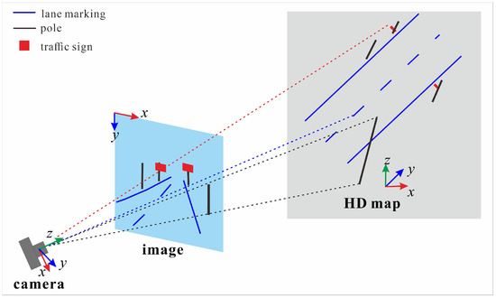
Figure 1. Schematic Representation of Camera-HD map Alignment.

Existing methods typically process input data without fully understanding its influence on localization performance. These approaches tend to focus on generating output directly, neglecting a thorough analysis of how different features in the scene contribute to registration accuracy. As a result, the varying importance of different object types and their impact on the final pose estimation are often overlooked. This limitation restricts the ability of these methods to adapt to diverse environmental conditions effectively.

A key challenge in image-to-HD map alignment lies in identifying the objects that significantly impact registration accuracy and prioritizing their importance. Among these objects, lane markings hold particular importance due to their strong geometric constraints. To address this, we introduce two key concepts: spatial distribution factors (SDFs) and spatial structural characteristics (SSC). SDF describes the spatial arrangement of objects in a scene, offering insights into the conditions that promote accurate and robust localization. SSC captures inherent geometric relationships and perspective transformations in image-HD map alignment, addressing challenges such as feature mismatches and variations in object scale. These concepts enhance the understanding of input data, forming the basis for improving registration accuracy and robustness.

The concept of SDF is inspired by its application in point cloud-to-point cloud map localization [1], where it predicts localization accuracy based on spatial characteristics of features. In this work, we extend and adapt this idea to the image-HD map alignment context, addressing the unique challenges of cross-modality registration. By combining SDF with SSC, we aim to enhance localization performance and improve robustness in challenging scenarios.

However, several challenges must be addressed, including identifying the feature types and scenarios that contribute to optimal localization, ensuring a uniform distribution of features for sensor data matching, and considering the positioning layer in HD maps [2,3]. Complex scenarios, such as at intersections where lane borders rely on human behavior, exacerbate these challenges, along with potential false negative visual detections, outdated map data, and abstract map representations designed to simplify geographic information.

By tackling these challenges, our research develops an enhanced object registration (EOR) that leverages SDF and SSC. The method aligns cameras with HD maps using object features such as lane markings, poles, and traffic signs. It quantifies the impact of feature distribution and refines geometric alignment during registration through carefully designed metrics that evaluate the spatial arrangement and positional accuracy of objects. The effectiveness of the EOR is validated through experiments on the open-source Argoverse 2 dataset [4]. The main contributions of this paper can be summarized as follows:

• SDF: Introduced to analyze the data distribution of objects in cross-modality visual images and HD map registration. These factors are designed to capture the varying importance of different object types and their contribution to localization accuracy and robustness.
• SSC: Proposed to enforce constraints during the optimization process, limiting abnormal solutions by leveraging inherent spatial relationships. These characteristics ensure geometric consistency and enhance alignment accuracy.
• EOR Framework: Developed to integrate SDF and SSC into a non-linear optimization framework that leverages insights from scenario features and object importance to improve localization accuracy and robustness.

The remainder of this paper is organized as follows: Section 2 reviews highly related works, Section 3 describes the proposed enhanced object registration method, Section 4 presents the experimental evaluation conducted on the Argoverse 2 dataset, Section 5 discusses the results of experiments, and finally, Section 6 concludes the paper, summarizing the key findings and discussing avenues for future research.

2. Related Work

2.1. Feature-Based Localization

In the field of feature-based localization for vehicle positioning and orientation estimation relative to a map, lane markings have been recognized as crucial features for autonomous localization in urban and highway environments. The lane-match method in [5] used a hybrid particle filter and factor graph to address ambiguities, demonstrating robustness on well-marked roads. Detected lane markings coupled with map data were used for ego-localization [6]. Furthermore, lane edges, including solid and dashed lane boundaries, are extracted from images and point clouds for cross-modality registration [7], where dashed lines compensate for inadequacies commonly found on highways. However, these methods heavily rely on the presence of lane markings, making them less reliable in environments with fewer or less visible lane markings.

To mitigate these limitations, several studies have integrated lane markings and curbs from both camera images and HD maps to achieve precise and robust localization [8]. Various features, including pole-like objects, traffic signs, and lane lines, were detected to match the light-weight HD map [9]. Lane markings, lane borders, curbs, traffic lights, and traffic signs are recognized from images [10] and implicitly associated with the HD map by applying a distance transform on binary images of each semantic class of interest.

However, in scenarios such as long, straight roads or intersections lacking distinct visual cues, positioning errors can still escalate due to limited feature availability. An accurate position estimation [11] was provided at intersections with ambiguous landmarks through maximum a posteriori determination. Lane markings, delimiters, and stop lines were extracted as the key information for intersection localization in [12]. Road markers, such as lane markers, stop lines, and traffic sign markers from a digital map, improved localization accuracy in [13]. Traffic lights were used to reduce localization errors in [14].

The studies listed in Table 1 provide a quantitative comparison of feature-based localization methods, highlighting their respective scenarios, accuracy, and key challenges. From the literature, there is a clear lack of emphasis on determining the relative importance of different feature types for registration accuracy. Most methods treat features equally without evaluating their individual contributions to pose estimation. This gap limits our understanding of which features are critical under different circumstances and how their availability affects robust localization. Our proposed approach seeks to overcome these limitations by enhancing robustness across diverse environments through a more comprehensive integration of multiple feature types and a deeper understanding of their contributions to localization accuracy.

Table 1. Comparison of Feature-Based Localization Methods for Autonomous Driving.

Study	Features Used	Scenario	Average Localization Error	Key Challenges
[5]	Lane markings	Well-marked roads	Lateral: 0.066 m, Longitudinal: 0.078 m	Over-reliance on lane markings
[6]	Lane markings	Urban/highway roads	Lateral: less than 0.10 m	Over-reliance on lane markings
[7]	Lane edges (solid, dashed)	Highway	Rotation: 0.3°, Translation: 0.05 m	Over-reliance on lane markings
[8]	Lane markings, curbs	Urban roads	Positioning: 0.19 m	Limited performance on roads or intersections lacking distinct features
[9]	Pole-like objects, traffic signs, and lane lines	Urban roads	Localization: 0.24 m	Feature matching error
[10]	Lane markings, lane borders, curbs, traffic lights, and traffic signs	Urban roads	Lateral: 0.19 m, Longitudinal: 0.70 m	Errors led by misclassification
[11]	Lane markings, ambiguous landmarks	Intersections	Lateral: 0.03 m, Longitudinal: 1.61 m	Ambiguity with limited feature availability
[12]	Lane markings, delimiters, stop lines	Intersections	Lateral: 0.32 m, Longitudinal: 0.20 m	Relies on stereo cameras
[13]	Lane markers, stop lines, traffic sign markers	Urban roads, intersections	Lateral: 0.076 m, Longitudinal: 0.53 m	Requires multiple computing threads
[14]	Traffic lights	Intersections	Lateral: 0.5 m, Yaw: <3°	Effective only at intersections

2.2. Map Quality Evaluation

Map quality evaluation is a crucial component for HD maps, with dimensions such as resolution, accuracy, completeness, and consistency previously outlined [15]. These evaluations, however, remain largely focused on individual map attributes without considering the complexities of integrating maps with sensor data from different modalities.

A framework for evaluating map quality in visual landmark-based mapping [1] used a convex hull approach to determine if query poses lie within regions observed by landmarks, providing a measure of spatial coverage. COLA and OSPA metrics [16] evaluate feature map quality in Simultaneous Localization and Mapping (SLAM). Normal distribution (ND) map quality is assessed through field testing [17]. Offline experiments estimate the uncertainty of 3D normal distribution transform (NDT) scan matching under varying environmental conditions. Criteria for evaluating ND maps for autonomous vehicle localization were introduced in [18], covering feature efficiency, layout, local similarity, and representation quality. Later, [19] extended this work to provide a more detailed modeling of the local similarity criterion, further refining the evaluation process.

These criteria are defined independently of specific map formats and can theoretically apply to various map types. However, their quantification primarily focuses on the ND map format, limiting practical applicability to other data modalities. These methods provide a quantitative judgment of the map representation abilities but are generally limited to single-modality maps, lacking an evaluation across multiple sensor modalities.

These existing evaluation methods, as shown in Table 2, do not fully account for the complex nature of data integration needed in cross-modality systems. Evaluating the quality of HD maps when combined with visual sensor data requires considering shared features, something missing in the existing body of literature.

Table 2. Evaluation Methods for Map Quality.

Study	Evaluation Method	Dimensions Assessed	Limitations
[15]	Quality Dimensions	Resolution, Accuracy	No integration with sensor data
[1]	Convex Hull-based Evaluation	Spatial Coverage, Visual Landmark Quality	Focused on visual landmark-based mapping
[16]	COLA & OSPA Metrics	Feature Map Quality	Focused on SLAM only
[17]	ND Map Field Testing	3D NDT Scan Matching, Uncertainty Assessment	Limited to pre-experiments
[18,19]	ND Map Criteria Evaluation	Feature Efficiency, Layout, Local Similarity, Representation Quality	Quantification primarily focused on the ND map format

3. Materials and Methods

The proposed EOR incorporates two types of spatial feature descriptions: SDF and SSC. The SDF provides insights into the overall feature distribution, guiding the registration process, while the SSC enforces specific geometric constraints to refine and optimize the registration results. This section will introduce the system overview, elaborate on key steps including image segmentation, SDF of objects from the HD map and images, SSC of HD map objects, and show the enhanced pose estimation.

3.1. System Overview

The proposed EOR system achieves precise alignment between visual images and HD maps by integrating multiple components to enhance localization accuracy and robustness, as depicted in Figure 2. The framework consists of key stages: input, preprocessing, pose initialization, feature analysis, and pose refinement, each contributing to the system’s overall effectiveness.

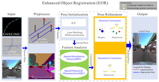
Figure 2. Framework of EOR.

The system begins with pose initialization, where the 3D Iterative Closest Point (ICP) algorithm [20] estimates an initial camera pose relative to the HD map. Feature analysis follows, extracting SDF from both visual images and HD maps, including feature occupancy, feature Geometric Dilution of Precision (GDOP), and longitudinal difference. These factors provide insights into the spatial configuration of objects and predictive measures of localization accuracy, based on criteria from [19]. Concurrently, SSC maintains geometric relationships during the camera’s perspective projection transformation.

In the pose refinement stage, SDF and SSC collaboratively optimize the initial pose estimate, thereby enhancing the overall alignment accuracy. Sequential operations for pose refinement are elaborated in Figure 3. To ensure temporal consistency across frames, an Extended Kalman Filter (EKF) [21] integrates pose estimations, reducing uncertainties and enhancing the consistency and robustness across dynamic sequences.

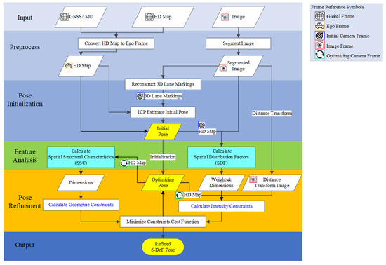
Figure 3. Detailed Flowchart of EOR.

Collectively, the EOR system leverages ICP, SDF, SSC, and EKF to iteratively refine pose estimations, achieving reliable and precise localization. Figure 2 and Figure 3 provide an overview and detailed breakdown of the EOR workflow, offering a comprehensive understanding of the methodology.

3.2. Image Segmentation and Postprocess

For visual semantic segmentation, two well-established networks are utilized to identify and isolate relevant entities. DeepLabv3 [22] is employed due to its highly regarded performance in semantic segmentation, specifically for extracting feature semantics related to poles and traffic signs. LaneNet [23] is utilized for segmenting lane markings. The Cityscapes dataset [24] and CULane dataset [25] are utilized to construct the initial training dataset.

Post-processing techniques, such as line fitting, are applied to refine the results of image semantic segmentation, particularly for lane markings and poles. Due to occlusions by vehicles, lane markings often experience a significant reduction in valid features, especially when dashed lines are occluded. Line fitting is an efficient and effective postprocess means for these kinds of cases. The segmented lane markings are projected to inverse perspective mapping, and lane counts are determined based on peaks along the x-axis. Lines are then fitted based on the collection of pixels within each lane, followed by transforming the fitted lane markings back to the original projective view. Similarly, line fitting is employed as a repair mechanism to address occlusions in the middle part of poles. Post-processing techniques are utilized to obtain rectangle bounding boxes for the traffic signs.

Furthermore, it is important to note that the segmentation results of poles and traffic signs, due to their small size, often exhibit increased noise to maintain a high recall ratio. However, these occasional miss-detections are relevant to the registration process, as they directly impact the accuracy of object alignment and localization.

3.3. Spatial Distribution Factors

The proposed SDF encompasses feature occupancy, feature GDOP, and longitudinal differences of relevant objects in both the visual images and the HD map. By analyzing the distribution and relative importance of features in the scene, SDF offers a comprehensive understanding of the spatial layout and coverage. This subsection presents the definition of 2D SDF from visual segmented images and 3D SDF from HD map objects, with a focus on lane markings, poles, and traffic signs. While their direct impact on registration will be further explored in the experiments section.

3.3.1. Feature Occupancy

Feature occupancy is utilized to assess the sufficiency of objects within the visual images and HD map. The feature occupancy 3D ${Occ}_{3d}^c$ is determined by image $I_m$ which is projected to the image plane from HD map $M_c$ in camera frame using (1):

$$I_m=\pi M_c$$

(1)

where $\pi$ represents the image perspective projection from the camera coordinate system to the image plane. This projection is formulated using the camera intrinsic matrix $\mathbf{K}$, given by (2):

$$\pi =\mathbf{K}\left[\begin{array}{c}{x}_c\\ y_c\\ z_c\end{array}\right]=\left[\begin{array}{ccc}{f}_x& 0& c_x\\ 0& f_y& c_y\\ 0& 0& 1\end{array}\right]\left[\begin{array}{c}{x}_c\\ y_c\\ z_c\end{array}\right]$$

(2)

where $f_x$ and $f_y$ are the focal lengths. $c_x$ and $c_y$ are the principal point offsets. $\left(x_c,y_c,z_c\right)$ is a point in the HD map $M_c$. This feature occupancy 2D ${Occ}_{2d}^c$ quantifies the ratio of occupied pixels by specific object categories $c$ relative to the total number of occupied pixels in the segmented image $I_s$, as shown in Figure 4a. ${Occ}_{2d}^c$ and ${Occ}_{3d}^c$ are calculated using (3):

$$\left\{\begin{array}{c}{Occ}_{2d}^c={\displaystyle \frac{Occ\left(I_s,c\right)}{Occ\left(I_s\right)}}\\ {Occ}_{3d}^c={\displaystyle \frac{Occ\left(I_m,c\right)}{Occ\left(I_m\right)}}\end{array}\right.$$

(3)

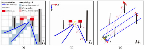
Figure 4. Diagram of Feature Occupancy and GDOP. (a) Occupancy 2D; (b) GDOP 2D; (c) GDOP 3D.

$Occ\left(I_s,c\right)$ represents the number of occupied grids for object category $c$ in the segmented image $I_s$. $Occ\left(I_s\right)$ represents the total number of occupied grids in $I_s$ (the union of all occupied grids across categories). Similarly, $Occ\left(I_m,c\right)$ and $Occ\left(I_m\right)$ are for the HD projected image $I_m$.

3.3.2. Feature GDOP

The feature GDOP, derived from GDOP [26], quantifies the level of geometric uncertainty associated with the positions of these features within the visual images and HD map. A lower feature GDOP indicates a higher level of confidence in the accuracy of the feature localization, while a higher feature GDOP suggests a higher degree of uncertainty. GDOP 2D is calculated in the image 2D coordinate system. The principal point $P\left(u,v\right)$ of the photography is taken as the center of feature 2D-DOP shown in Figure 4b. GDOP 3D is calculated in the camera 3D coordinate system shown in Figure 4c. The ${GDOP}_{2d}$ and ${GDOP}_{3d}$ are obtained using (4):

$$\left\{\begin{array}{c}{GDOP}_{2d}=\sqrt{tr{\left({H_{2d}}^T{H}_{2d}\right)}^{-1}}\\ {GDOP}_{3d}=\sqrt{tr({H_{3d}}^T{H}_{3d}{)}^{-1}}\end{array}\right.$$

(4)

where $tr\left(\right)$ represents the trace of a matrix referring to the sum of the elements on the main diagonal. $H_{2d}$ and $H_{3d}$ are given by (5):

$$\left\{\begin{array}{c}{H}_{2d}=\left(\begin{array}{cc}{\displaystyle \frac{x_1-u}{r_1}}& {\displaystyle \frac{y_1-v}{r_1}}\\ {\displaystyle \frac{x_2-u}{r_2}}& {\displaystyle \frac{y_2-v}{r_2}}\\ ⋮& ⋮\\ {\displaystyle \frac{x_m-u}{r_m}}& {\displaystyle \frac{y_m-v}{r_m}}\end{array}\right)\\ H_{3d}=\left(\begin{array}{ccc}{\displaystyle \frac{x_1-x_c}{r_1}}& {\displaystyle \frac{y_1-y_c}{r_1}}& {\displaystyle \frac{z_1-z_c}{r_1}}\\ {\displaystyle \frac{x_2-x_c}{r_2}}& {\displaystyle \frac{y_2-y_c}{r_2}}& {\displaystyle \frac{z_2-z_c}{r_2}}\\ ⋮& ⋮& ⋮\\ {\displaystyle \frac{x_m-x_c}{r_m}}& {\displaystyle \frac{y_m-y_c}{r_m}}& {\displaystyle \frac{z_m-z_c}{r_m}}\end{array}\right)\end{array}\right.$$

(5)

where $r$ for $H_{2d}$ is the distance between the pixel $\left(x,y\right)$ and the principal point $\left(u,v\right)$. $r$ for $H_{3d}$ is the distance between the point $\left(x,y,z\right)$ and the camera position $\left(x_c,y_c,z_c\right)$. $m$ is the total number of the key points.

3.3.3. Longitudinal Difference

The longitudinal accuracy is not easy to handle because the local environment similarity shows the chance of getting stuck at a local optimum. The similarity estimation of the local environment is achieved by comparing the image similarity between the projected HD map image $M_c$ and the segmented image $I_s$. This comparison is performed using exhaustive map translation $t$ in the longitudinal direction in Figure 5a. The translated maps project onto the image plane as in Figure 5b. The similarity metric ${IoU}_i$ utilizes the $IoU$ [27] of the two images in the $i$-th iteration. The entropy of similarity $L_i$ denotes the distribution of ${IoU}_i$ among these exhaustive steps calculated using (6):

$$\left\{\begin{array}{c}{IoU}_i=IoU\left(I_s,\pi \left(M_c,t_i\right)\right)\\ L_i=-\sum _{i}p\left({IoU}_i\right)logp\left({IoU}_i\right)\end{array}\right.$$

(6)

Figure 5. Diagram of Longitudinal Difference. (a) Longitudinal Translation; (b) Project onto Image.

3.4. Spatial Structural Characteristics

The registration between the on-vehicle images and the HD map involves aligning data from different spaces and modalities. Due to the characteristics of perspective projection, certain structural traits remain unchanged or transform into other characteristics. To capture these spatial structural transformations in the 3D-2D registration, we defined category-based SSC.

According to [28], guiding principles based on the Law of Parallel Lines in Perspective provide a framework for understanding these spatial transformations. These principles state that parallel lines that are parallel to the picture plane remain parallel in the perspective view, while parallel lines perpendicular to the picture plane converge towards a vanishing point, as displayed in Figure 6a. In the context of the registration process, the shapes of lane markings belong to the category of parallel lines that converge towards a vanishing point. Meanwhile, poles and traffic signs fall under the category of parallel lines that remain parallel, as shown in Figure 6b–d. Assuming that the shapes of the HD map objects in the camera frame are composed of points $\left(x_c,y_c,z_c\right)$, we can represent the object category-based factors as follows.

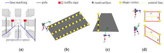
Figure 6. SSC of HD Map Objects. (a) Map objects in parallel perspective space; (b) Lane markings; (c) Poles; (d) Traffic signs.

3.4.1. Lane Markings

Lane markings within the local region of interest in the camera coordinate system are positioned in a plane parallel to the x–z plane, as depicted in Figure 6b. The small standard deviation of the camera coordinate along the y-axis $y_c$ values indicates that the lane markings remain parallel to the road surface. This implies that they maintain a consistent height relative to the camera and do not significantly deviate from the parallel x–z plane. These characteristics are represented using the standard deviation, as given by (7):

$${SSC}_{lm}=\begin{array}{c}std\left(y_c\right)\end{array}$$

(7)

3.4.2. Poles

Poles observed in the camera coordinate system exhibit a perpendicular alignment to the x-axis, as depicted in Figure 6a,c. This indicates that the poles are positioned vertically or nearly vertically with respect to the camera’s field of view. The points forming a pole concentrate along the x-axis, showing minimal horizontal variation relative to the camera. Moreover, the points of a pole share an approximate depth, resulting in a narrow distribution along the depth axis. These characteristics can be represented using the standard deviations, using (8):

$${SSC}_{pole}=\left\{\begin{array}{c}std\left(x_c\right)\\ std\left(z_c\right)\end{array}\right.$$

(8)

3.4.3. Traffic Signs

Traffic signs have various shapes, such as rectangles, triangles, circles, or other polygons. To represent their spatial structure, we use bounding boxes, which are rectangles that encompass the entire shape. When observing a traffic sign object facing the picture plane, the points of the traffic sign are located at a relatively consistent depth in the camera coordinate system. The bounding box has parallel upper and lower edges to the x-axis, while parallel left and right edges to the y-axis, as shown in Figure 6d. Then the central horizontal line shows concentration along the y-axis, while the central vertical line shows concentration along the x-axis. These characteristics can be quantified using standard deviations, as given by (9):

$${SSC}_{sign}=\left\{\begin{array}{c}\begin{array}{c}std\left(x_c^v\right)\\ std\left(y_c^h\right)\\ std\left(z_c\right)\end{array}\end{array}\right.$$

(9)

3.5. Enhanced Pose Estimation

The proposed pose estimation belongs to an optimization-based method. It starts with the initial estimation using 3D ICP and subsequently refines the estimated camera pose using the SDF and SSC, as depicted in Figure 2.

3.5.1. ICP Pose Initialization

To obtain a relatively good initialization, we utilized the 3D ICP technique on the 3D reconstruction of image lane markings and HD map lane markings. A simple 3D reconstruction calculation is executed on image lane markings based on the camera model, as shown in Figure 7a. We manually choose two points, p1 $\left(u_1,v_1\right)$ and p2 $\left(u_2,v_2\right)$ on parallel lane markings from the image, measure physical lane width $w$ (${w=x}_{c1}-x_{c2}$) of the corresponding point pair p1 $\left(x_{c1},y_{c1},z_{c1}\right)$ and p2 $\left(x_{c2},y_{c2},z_{c2}\right)$ from the HD map. We use vector $A_{3\times 1}$ to represent the transformation from point $\left(u,v\right)$ to $\left(x_c,y_c,z_c\right)$, as described by (10):

$$\left(\begin{array}{c}{\displaystyle \frac{x_c}{z_c}}\\ {\displaystyle \frac{y_c}{z_c}}\\ 1\end{array}\right)=K^{-1}\left(\begin{array}{c}u\\ v\\ 1\end{array}\right)=A_{3\times 1}$$

(10)

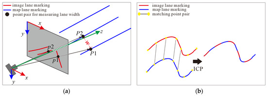
Figure 7. 3D ICP Process on Lane Marking Points. (a) Calculation of Camera Height; (b) 3D ICP.

Use $\alpha$ to record $x_c/y_c$ with (11):

$$\alpha ={\displaystyle \frac{x_c}{y_c}}={\displaystyle \frac{A_0}{A_1}}$$

(11)

Then the camera equipped height $h$ can be obtained according to (12):

$$h=y_c={\displaystyle \frac{w}{{\alpha }_1-{\alpha }_2}}$$

(12)

The image lane markings can be reconstructed to the 3D camera frame using the obtained $\left(x_c,y_c,z_c\right)$ coordinates. A general ICP procedure shown in Figure 7b is executed between the reconstructed lane markings and the local HD map in the 3D ego frame to estimate the pose between the camera frame and the ego frame. The resulting camera pose is then used as an initialization value of EKF for the subsequent precise alignment.

3.5.2. Enhanced Pose Optimization

To maximize the advantages of combining multiple sources of information, we enhance the pose optimization by integrating SDF and SSC with traditional intensity constraints on distance transform images [10]. We assume the object categories $C=\left[lanemarking,pole,sign\right]$. The process begins by extracting the binary image $B_c$ for each object category $c\left(c\in C\right)$ from the segmented image. Using OpenCV [29], we calculate the distance transform image $D_c$ on $B_c$ and normalize it to the range [0, 1]. The pose P ($P\in \mathrm{S}\mathrm{E}\left(3\right)$) represents the 6-DoF transformation from the ego to the camera frame, encompassing both translational and rotational components. The target of this enhanced pose optimization module is to construct the cost function $\xi \left({\rm P}\right)$ using SDF and SSC to solve for P. The point $p,\mathrm{P}p$, and $\pi \mathrm{P}p$ correspond to the HD map objects in the ego, camera, and image coordinate systems, respectively, with the category $c$. $\xi \left({\rm P}\right)$ comprises two parts: the intensity cost function $I$ and the geometric cost function $G$, as expressed in (13):

$$\begin{gathered} \xi \left({\rm P}\right)=\sum _{pϵS,c\in C}I\left(p,c\right)+\alpha ·G\left(p,c\right) \\ =\sum _{pϵS,c\in C}I\left(\pi Pp,c\right)+\alpha ·G\left(Pp,c\right) \end{gathered}$$

(13)

where $\alpha$ is a weight parameter for the balance between the intensity constraint and the geometric constraint. $I\left(p,c\right)(I\in \left[\mathrm{0,1}\right])$ is the intensity difference at each pixel $p_i\left(u,v\right)$ between the distance segmented image $D_c$ and the projected HD map image, as described by (14):

$$I\left(p,c\right)=1.0-D_c\left(f_{SDF}\left(p,c\right)\right)$$

(14)

When $I\left(p,c\right)=0$, it indicates that the map point $p$ perfectly aligns with a segmented feature in $D_c$. On the other hand, when $I\left(p,c\right)=1$, it means $p$ is projected onto a blank area of $D_c$. The function $f_{SDF}\left(p,c\right)$ maps the inputs to the corresponding object weights and optimized dimensions, as given in (15):

$$f_{SDF}\left(p,c\right)=\left(w_{lm},w_{pole},w_{sign},d\right)$$

(15)

Here, $w_{lm}$, $w_{pole}$, and $w_{sign}$ denote the weights assigned to each object category. $d$ represents the optimized dimensions within the 6-DoF using a specific index:$\left(\mathrm{0,1},\mathrm{2,3},\mathrm{4,5}\right)$ corresponds to $\left(x,y,z,pitch,yaw,roll\right)$, respectively.

As shown in Table 3, the initial weights for lane markings and poles are set to 1.0, indicating their importance as reference objects. The weight for traffic signs is set to 0.5, considering the potential limitations of bounding box post-processing and manual labeling procedures from LiDAR point clouds, which may not capture the complete shape of the signs. The initial dimensions contain 6-DOF.

Table 3. Cost Function Composition and Constraints.

Scenario	SDF Values	Weights and Dimensions
Initialization	/	$\left\{\begin{array}{c}{\left(w_{lm},w_{pole},w_{sign}\right)}_0=\left(\mathrm{1.0,1.0,0.5}\right)\\ d_0=\left(\mathrm{0,1},\mathrm{2,3},\mathrm{4,5}\right)\end{array}\right.$
Condition (1)	${\mathrm{O}\mathrm{c}\mathrm{c}}_{3d}^c=0$ or ${\mathrm{O}\mathrm{c}\mathrm{c}}_{2d}^c=0$	$\begin{array}{c}{w}_c=0\end{array}$
Condition (2)	$L_{lm}<l$	$\left\{\begin{array}{c}\left(w_{pole},w_{sign}\right)={2\left(w_{pole},w_{sign}\right)}_0\\ d=\left(\mathrm{3,4},5\right)\end{array}\right.$
Condition (3)	$L_{lm}\ge l$ and ${\mathrm{O}\mathrm{c}\mathrm{c}}_{3d}^c>{\mathrm{O}\mathrm{c}\mathrm{c}}_{3d}^{lm}$	$\left(w_{pole},w_{sign}\right)={2\left(w_{pole},w_{sign}\right)}_0$
Condition (4)	$L_c<l$	$d=\left(\mathrm{0,1},\mathrm{3,4},5\right)$
Condition (5)	$G{DOP}_{2d}^c>g or$ $G{DOP}_{3d}^c>g$	$w_c=0.5 w_{c0}$

The adjustment of object weights and optimized dimensions based on different scenario conditions 1~5 can be summarized as follows:

• If the object category occupancy ratio ${\mathrm{O}\mathrm{c}\mathrm{c}}_{3d}^c=0$ or ${\mathrm{O}\mathrm{c}\mathrm{c}}_{2d}^c=0$: Set the weight assigned to that category to 0. This adjustment is due to the absence of occupancy in the respective modality, which restricts the ability to establish meaningful relationships or constraints between modalities.
• If the longitudinal difference of lane markings $L_{lm}<l(l=0.1)$: Increase the weights for poles and traffic signs and prevent the optimization of translation. $L_{lm}<l$ ($l=0.1$) indicates the vehicle’s location entering a road intersection. This accounts for unreliable lane markings in intersections, prioritizing independent objects and preserving spatial relationships.
• If the longitudinal difference of lane markings $L_{lm}\ge l(l=0.1)$ and ${\mathrm{O}\mathrm{c}\mathrm{c}}_{3d}^c>{\mathrm{O}\mathrm{c}\mathrm{c}}_{3d}^{lm}$: Increase the weights for poles and traffic signs. This compensates for unreliable lane markings in normal road sections, enhancing the influence of poles and traffic signs in the analysis.
• If the longitudinal difference of object $L_c<l(l=0.1)$: Prevent longitudinal translation. This accounts for objects with a high degree of similarity in their longitudinal distribution, maintaining their relative positions during the optimization process.
• If the spatial distribution $G{DOP}_{2d}^c>g orG{DOP}_{3d}^c>g (g=0.4)$: Decrease weights of all categories. This accounts for unbalanced object distributions, helping to mitigate potential registration errors in the pose estimation process.

The geometric cost function $G\left(p,c\right)$ is composed of several standard deviations with the details in Section 3.4, as given by (16). The residual block of $G\left(p,c\right)$ is typically around 0.001. The geometric properties of map objects remain unaffected by the translation dimensions of the 6-DOF pose.

$$G\left(p,c\right)=f_{SSC}\left(p,c\right)=\left\{\begin{array}{l}{SSC}_{lm}\left(c=lanemarking\right)\\ {SSC}_{pole}\left(c=pole\right)\\ {SSC}_{sign}\left(c=sign\right)\\ d=\left(\mathrm{3,4},5\right)\end{array}\right.$$

(16)

The mentioned values $\alpha =100$, $l=0.1\left(lϵ\left(\mathrm{0,1}\right)\right)$, and $g=0.4$ $\left(gϵ\left(\mathrm{0,1}\right)\right)$ are determined based on the theoretical range and experimental observations. Ceres Solver [30] is employed to facilitate the optimization process. Bi-cubic interpolation is used on the distance transform image to get a smooth gradient. The SoftOneLoss function is used to decrease the impact of outliers. The distance parameters are constrained within the range of [−1.5, 1.5] meters, while the altitude angle parameters are bounded within [−0.2, 0.2] radians.

3.5.3. EKF Pose Fusion

In the proposed EOR method, the EKF integrates pose estimations across frames, enhancing system robustness and accuracy. For the first frame, a 3D ICP algorithm determines the initial pose. This pose undergoes refinement and is used to initialize the EKF for state prediction and error estimation. For subsequent frames, the EKF predicts an initial pose, which is refined to adapt to the current scene. The EKF then updates the pose by integrating the refined result with previous estimates, reducing uncertainty and ensuring a stable trajectory. This EKF-based pose fusion maintains smooth localization, especially in challenging environments requiring rapid adjustments. The process, including initialization, prediction, refinement, and updates, is outlined in the flowchart in Figure 8.

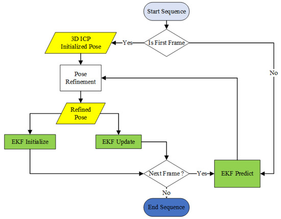
Figure 8. Flowchart of EKF Pose Fusion.

4. Experiments

In order to validate the effectiveness of the proposed registration method, we conducted experiments using the Argoverse 2 dataset [4]. The dataset provides sequential visual images, frame-by-frame LiDAR point clouds, 3D HD vector maps, and accurate pose information for both images and LiDAR point clouds with respect to the HD maps. The utilized two sequences were collected in Miami (Figure 9a) and DTW (Figure 9b), covering a distance of 200 and 600 m, respectively. In the first sequence, the environment is situated under an overpass bridge. The presence of pillars and nearby buildings can potentially lead to misrecognition of poles and signs. The second sequence features a wider road with multiple lanes and an increased number of poles. The sequences are depicted overlapping with OpenStreetMap in Figure 7, serving as a geospatial reference for the collected data.

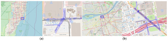
Figure 9. Overview of Experimental Data of Argoverse. (a) Sequence 1 in Miami (b) Sequence 2 in DTW.

The evaluation experiments are divided into five parts. Firstly, we describe the specific data preprocessing steps, including labeling poles and traffic signs from LiDAR point clouds and postprocessing on the image segmentation results. Next, we present the results of the random experiments, followed by the sequential experiments, which compare the performance of the lane marking-only registration method (VisionHD) [27], an existing multi-object registration method (MOR) [10], and the proposed EOR method. Subsequently, we conduct an ablation study evaluating the contributions of SDF, SSC, and key feature types (lane markings, poles, and traffic signs) to localization performance. Finally, we assess the computation time of key modules to evaluate the efficiency of the registration method.

To ensure a fair comparison, all methods in our experiments utilize the ICP process for pose initialization. We implemented the compared methods by ourselves, following the principles described in the literature. To ensure clear presentation and effective comparison of the results, we employ several metrics for robustness and accuracy evaluation. The robustness metric measures the probability of achieving successful registration, indicating the method’s reliability. The accuracy assessment includes classic 6-DoF pose errors, which provide a measure of the registration accuracy in terms of translation (along X, Y, and Z axes), and rotation (in roll, pitch, and yaw). Additionally, we employ Intersection over Union (IoU) values [27] based on the registered HD map and segmented image. A high IoU value indicates a high registration accuracy, while a low value suggests misalignment. These metrics enable effective comparisons with other registration approaches.

4.1. Data Preprocessing

The data preprocessing stage involves two main steps: manual extraction of map objects and postprocessing of segmented objects. The HD vector map in the open-source Argoverse2 dataset provides detailed 3D information about lane markings. However, information about poles, traffic signs, and other roadside infrastructures is unavailable. To address this limitation, we performed manual annotation of poles and traffic signs within the experimental regions using the open-source CloudCompare software (version 2.11.3) [31]. This annotation was carried out on the LiDAR point clouds, which were transformed from the LiDAR coordinate system to the global coordinate system with the provided corresponding sensor poses. The annotation followed specific principles:

• Only features within 20 m of the road surface were collected;
• Only visible points were considered for collection;
• The bottom of poles reached the lowest visible point, and the top of poles ended before any curvature, if present;
• Traffic signs were collected at the four corners.

The human-annotated process of map objects is depicted in Figure 10. Figure 10a provides an overview of the transformed LiDAR point clouds. Figure 10b provides partial enlarged details of these annotated poles and traffic signs, allowing for a closer examination. Additionally, Figure 10c presents a 2D orthophoto perspective view of the HD map objects in a specific area, providing a visual representation of the registered objects within the map context.

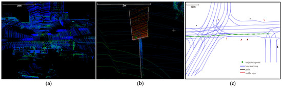
Figure 10. Manual Annotated Process of Poles and Traffic Signs. (a) Accumulated Point Clouds; (b) Annotation; (c) Ortho View.

4.2. Random Experiment

The Random Experiment evaluated the performance of our method by generating abundant variations in camera pose for a single captured image frame. It aims to quantify the probability of retrieving a good pose by randomly sampling different camera poses.

Table 4 summarizes the mean translation errors, rotation errors, and IoU results for EOR, MOR, and VisionHD, while Figure 11 provides visual insights into the error distributions and alignment performance across all dimensions (x, y, z, pitch, yaw, roll) and IoU. From Table 4, VisionHD achieves the lowest x-axis translation error (0.14 m), indicating superior lateral precision due to its reliance on lane markings. However, this comes at the cost of larger z-axis errors (2.47 m), highlighting its limitation in controlling longitudinal accuracy. The proposed EOR method achieves balanced performance across all dimensions. It reduces the mean z translation error to 1.48m and achieves comparable IoU (0.28) to MOR. Notably, EOR improves robustness with a 90% probability of IoU > 0.2, outperforming MOR (87%) and VisionHD (65%). The red shade in Figure 11c highlights the IoU > 0.2 range.

Table 4. Random Experiment Errors and IoU.

Method	Mean Translation Errors			Mean Rotation Errors			IoU	P (IoU > 0.2)
	x (m)	y (m)	z (m)	Pitch (rad)	Yaw (rad)	Roll (rad)
SampleInit	0.48	0.44	0.46	0.05	0.05	0.05	0.04	1%
EOR	0.18	0.21	1.48	0.01	0.01	0.02	0.28	90%
MOR	0.20	0.24	1.29	0.01	0.01	0.03	0.28	87%
VisionHD	0.14	0.24	2.47	0.01	0.01	0.03	0.24	65%

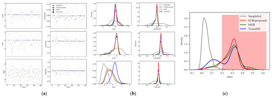
Figure 11. Random Experiment Result. (a) Scatter Distribution of 6-DoF Errors; (b) KDE Distribution of 6-DoF Errors; (c) KDE Distribution of IoU.

Figure 11a,b visualize the error distributions and show that registered errors in all dimensions, except z, regress towards zero, demonstrating improved alignment. Figure 11c further highlights the overall alignment trends, reinforcing the quantitative results presented in Table 4.

4.3. Sequential Experiment

The Seqential Experiment aimed to assess the method’s performance along a predefined trajectory, encompassing various environmental conditions, viewpoints, and image recognition scenarios. It provided insights into the consistency, accuracy, and robustness of the methods in real-world scenarios. Two sequential trajectories from the Argoverse dataset were used for the experiments.

Figure 12 shows the qualitative results using the proposed EOR method, employing the projection of HD map objects onto images for quantitative analysis. The displayed frames represent different stages: approaching an intersection, inside the intersection, and leaving the intersection. In the frames approaching an intersection, where lane markings and poles are abundant, we observed relatively good and steady registration results. However, frames captured inside the intersections, where only poles and some signs were available for registration, introduced challenges.

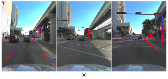
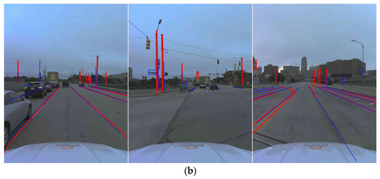
Figure 12. Qualitative Results of EOR method. The columns are approaching, inside and leaving intersection respectively. (a) Sequence 1; (b) Sequence 2.

Figure 13 illustrates the sequential SDF values alongside the IoU values. The upper blue part of the figure represents the SDF values, including occupancy 3D, occupancy 2D, GDOP 3D, GDOP 2D, and the longitudinal difference of respective object categories. While the lower white part shows the registered IoU values. The red shaded regions indicate intersection areas. From Figure 13, we observe that the occupancy of lane markings decreases inside the intersections, while the occupancy of poles increases. Traffic signs tend to appear at a distance along the road. However, lane markings’ occupancy does not always decrease to zero within the intersection area, as different crossroads and T-junctions may have various patterns of painted lane markings. The occupancy 3D and occupancy 2D, as well as GDOP 3D and GDOP 2D, exhibit similar trends but not always identical.

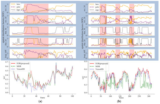
Figure 13. SDF Values and Quantitative IoU Results. (a) Sequence 1; (b) Sequence 2.

Table 5 provides a quantitative comparison of the mean translation errors, rotation errors, and IoU values across two sequences. For Sequence 1, the EOR and MOR methods have similar and higher mean IoU (0.32 and 0.33, respectively), compared to VisionHD (0.29). This suggests that both EOR and MOR methods produce similar overall registration results in Sequence 1. However, EOR exhibits significantly lower errors in the y and z directions (0.19 m and 0.94 m) compared to MOR (0.49 m, 1.46 m) and VisionHD (0.19 m, 1.45 m). This highlights the robustness of EOR, particularly in longitudinal (z) control.

Table 5. Sequence Experiment Errors and IoU.

Scenario	Method	Mean Translation Errors			Mean Rotation Errors			IoU
		x (m)	y (m)	z (m)	Pitch (rad)	Yaw (rad)	Roll (rad)
Sequence 1	EOR	0.21	0.19	0.94	0.02	0.01	0.03	0.32
	MOR	0.29	0.49	1.46	0.02	0.01	0.04	0.33
	VisionHD	0.22	0.19	1.45	0.02	0.01	0.02	0.29
Sequence 2	EOR	0.10	0.07	0.37	0.00	0.01	0.01	0.37
	MOR	0.50	0.65	2.10	0.02	0.02	0.04	0.27
	VisionHD	0.15	0.08	2.16	0.01	0.01	0.01	0.33

For Sequence 2 in Table 5, EOR achieves the highest mean IoU (0.37), surpassing MOR (0.27) and VisionHD (0.33), indicating superior overall registration performance. Notably, EOR achieves the lowest errors across all six dimensions, with mean errors of 0.10 m (x), 0.07 m (y), and 0.37 m (z) in translation, as well as 0.01 radians in rotation.

Figure 14 visualizes the 6-DoF errors for both sequences. Figure 14a confirms EOR’s superior accuracy, particularly in the y and z directions for Sequence 1. For Sequence 2, Figure 14b corroborates the results from Table 5, showing that EOR consistently outperforms the other methods across all dimensions, despite occasionally exhibiting high yaw error values.

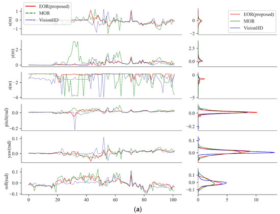
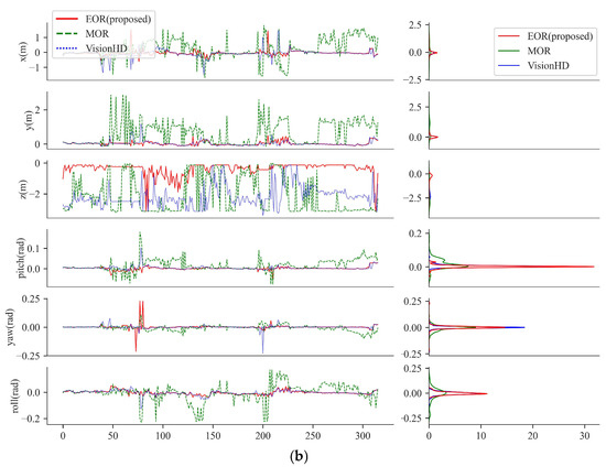
Figure 14. Quantitative Result: 6-DoF errors. (a) Sequence 1; (b) Sequence 2.

4.4. Ablation Study

To evaluate the effectiveness of key components and feature types in the proposed method, we conducted two ablation studies. The first study isolates the contributions of SDF and SSC by systematically excluding them or using each component individually. The second study investigates the impact of feature types, including lane markings, poles, and traffic signs, by testing combinations of these features.

Table 6 shows the results of the component ablation study. The “base” method, which combines SDF and SSC, achieves the lowest translation and rotation errors, demonstrating the importance of integrating both components. Excluding all components (“exclude-all”) leads to the worst performance, particularly in elevation (z) and yaw, confirming the necessity of these spatial factors. SDF alone performs slightly better in z compared to SSC alone, while SSC shows better performance in rotation accuracy.

Table 6. Ablation Results for Components.

Method	Mean Translation Errors			Mean Rotation Errors			IoU
	x (m)	y (m)	z (m)	Pitch (rad)	Yaw (rad)	Roll (rad)
base	0.21	0.19	0.94	0.02	0.01	0.03	0.32
exclude-all	0.33	0.49	1.38	0.02	0.02	0.05	0.31
SDF-only	0.3	0.33	1.1	0.02	0.02	0.05	0.31
SSC-only	0.29	0.42	1.34	0.02	0.01	0.02	0.33

Table 7 presents the results for feature type combinations. Lane markings alone deliver reasonable accuracy but are less robust in elevation (z). Adding poles improves accuracy across all dimensions due to their spatial consistency in urban scenes. Combining lane markings with traffic signs yields lower IoU and higher z error, highlighting that traffic signs alone are less effective than poles for precise registration. These findings emphasize the critical role of feature combinations in robust localization.

Table 7. Ablation Results for Feature Types.

Method	Mean Translation Errors			Mean Rotation Errors			IoU
	x (m)	y (m)	z (m)	Pitch (rad)	Yaw (rad)	Roll (rad)
base	0.21	0.19	0.94	0.02	0.01	0.03	0.32
lane	0.22	0.18	1.47	0.01	0.01	0.02	0.28
lane+pole	0.24	0.24	0.93	0.02	0.01	0.03	0.32
lane+trafficsign	0.23	0.2	1.47	0.02	0.02	0.02	0.28

4.5. Computation Time

The system is running on Windows 10 with an Intel Core i7-8700 CPU. The segmentation module, however, is independent from the main thread and runs on an NVIDIA Quadro P4000 GPU. The input image size is 1550 × 2048. Table 8 provides a breakdown of the time consumption for different modules within the system.

Table 8. Running Time Statistics.

Module	Average Time (s)
Lane markings segmentation by LaneNet	0.013
Objects segmentation by DeepLabv3	1.5
ICP pose initialization	0.01
SDF calculation	0.01
SSC calculation	0.001
Intensity constraint on distance transform	0.002
Pose optimization	0.08
EKF	0.001

5. Discussion

5.1. Robustness and Accuracy from Random and Sequential Experiments

The EOR method demonstrates strong robustness through both random and sequential experiments, combining information from multiple object types. Lane markings provide strong cues for lateral alignment, while poles enhance longitudinal alignment. The EOR method particularly enhances longitudinal precision and IoU success rates through its integration of multiple feature types.

From a sequential perspective, EOR effectively handles challenging scenarios like intersections where lane markings may be absent. Frames leaving intersections showed well-aligned registration, suggesting effective use of features, even when lane markings were distant. Additionally, the EKF plays a vital role in minimizing uncertainties, ensuring smoothed trajectories, and reducing the impact of recognition errors across frames. These contributions collectively enhance robustness in complex environments. Additionally, EOR consistently outperformed baselines, demonstrating superior accuracy in all six dimensions.

Occasional peaks in yaw error, observed in Sequence 2 when approaching intersections, highlight scenarios where the absence of lane markings forces reliance on poles and traffic signs. However, poles and traffic signs are relatively small and prone to imperfect recognition, which can introduce potential errors in the registration process. Despite these peaks, the sequence-average yaw error remained low, with the EOR method achieving an average error of 0.01 radians—comparable to VisionHD and better than MOR at 0.02 radians. This consistency in average error reinforces EOR’s robustness and adaptability to diverse scenarios.

5.2. Scene Understanding from Sequential Experiments

The sequential experiments reveal additional scene-understanding capabilities provided by the spatial factors. HD map-derived 3D factors exhibit smoother and more consistent trends compared to segmented image-derived 2D factors, primarily due to the inherent noise in visual recognition. The GDOP factor, which generally indicates low uncertainty when objects are evenly distributed, becomes larger when there is clustering or a lack of objects, indicating possible registration challenges. The longitudinal difference factor aligns well with intersection regions, serving as a reliable indicator of intersection boundaries. These findings demonstrate the role of spatial factors in enhancing scene understanding and providing insights into the distribution and quality of environmental features.

5.3. Insights from Ablation Studies

The ablation study provides valuable insights into the contributions of different components and feature types to the EOR performance. The component ablation study results demonstrate that combining SDF and SSC achieves the highest accuracy across translation, rotation, and IoU dimensions. Removing both components severely impacts performance, particularly in the z-axis and yaw angle, emphasizing their importance. SDF is more effective for z-axis accuracy due to its analysis of spatial object distribution, while SSC significantly enhances rotation accuracy by enforcing geometric consistency.

The feature type ablation study results indicate that lane markings alone provide reasonable localization accuracy but are insufficient for longitudinal alignment. Adding poles significantly enhances overall accuracy, especially at intersections, due to their spatial stability. Combining lane markings with traffic signs leads to higher z errors and a lower IoU, indicating that traffic signs are less effective for robust registration compared to poles. These findings emphasize the importance of a well-balanced combination of feature types, such as lane markings, poles, and traffic signs, for optimal localization performance.

6. Conclusions

This research presents an EOR method that leverages SDF and SSC to improve the accuracy and robustness of object registration in autonomous driving systems. Extensive experimentation was conducted to assess the impact of feature occupancy, feature GDOP, and longitudinal difference on the registration process. The results validate the effectiveness of the proposed EOR in maintaining lateral and elevation accuracy, enhancing longitudinal accuracy, and increasing the probability of successful registration. Future work could focus on further refining the EOR, exploring additional factors that influence object registration, and expanding the experimentation to diverse real-world scenarios to validate the method’s effectiveness and applicability.

References

- Merzic, H.; Stumm, E.; Dymczyk, M.; Siegwart, R.; Gilitschenski, I. Map quality evaluation for visual localization. In Proceedings of the 2017 IEEE International Conference on Robotics and Automation, Singapore, 29 May–3 June 2017; pp. 3200–3206. [Google Scholar]
- Ying, S.; Jiang, Y.; Gu, J.; Liu, Z.; Liang, Y.; Guo, C.; Liu, J. High Definition Map Model for Autonomous Driving and Key Technologies. Geomat. Inf. Sci. Wuhan Univ. 2024, 49, 506–515. [Google Scholar] [CrossRef]
- Poggenhans, F.; Salscheider, N.O.; Stiller, C. Precise Localization in High-Definition Road Maps for Urban Regions. In Proceedings of the 2018 IEEE/RSJ International Conference on Intelligent Robots and Systems, Madrid, Spain, 1–5 October 2018; pp. 2167–2174. [Google Scholar]
- Wilson, B.; Qi, W.; Agarwal, T.; Lambert, J.; Singh, J.; Khandelwal, S.; Pan, B.; Kumar, R.; Hartnett, A.; Pontes, J.K.; et al. Argoverse 2: Next Generation Datasets for Self-Driving Perception and Forecasting. arXiv 2023, arXiv:2301.00493. [Google Scholar]
- He, M.; Rajkumar, R.R. LaneMatch: A Practical Real-Time Localization Method Via Lane-Matching. IEEE Robot. Autom. Lett. 2022, 7, 4408–4415. [Google Scholar] [CrossRef]
- Gruyer, D.; Belaroussi, R.; Revilloud, M. Map-aided localization with lateral perception. In Proceedings of the IEEE Intelligent Vehicles Symposium Proceedings, Dearborn, MI, USA, 8–11 June 2014; pp. 674–680. [Google Scholar]
- Jiang, Z.; Cai, Z.; Hui, N.; Li, B. Multi-Level Optimization for Data-Driven Camera–LiDAR Calibration in Data Collection Vehicles. Sensors 2023, 23, 8889. [Google Scholar] [CrossRef] [PubMed]
- Tao, Z.; Bonnifait, P.; Frémont, V.; Ibanez-Guzman, J.; Bonnet, S. Road-Centered Map-Aided Localization for Driverless Cars Using Single-Frequency GNSS Receivers. J. F. Robot. 2017, 34, 1010–1033. [Google Scholar] [CrossRef]
- Xiao, Z.; Yang, D.; Wen, T.; Jiang, K.; Yan, R. Monocular localization with vector HD map (MLVHM): A low-cost method for commercial IVs. Sensors 2020, 20, 1870. [Google Scholar] [CrossRef] [PubMed]
- Pauls, J.-H.; Petek, K.; Poggenhans, F.; Stiller, C. Monocular Localization in HD Maps by Combining Semantic Segmentation and Distance Transform. In Proceedings of the 2020 IEEE/RSJ International Conference on Intelligent Robots and Systems, Las Vegas, NV, USA, 25–29 October 2020; pp. 4595–4601. [Google Scholar]
- Mattern, N.; Wanielik, G. Camera-based vehicle localization at intersections using detailed digital maps. In Proceedings of the IEEE PLANS, Position Location and Navigation Symposium, Indian Wells, CA, USA, 3–6 May 2010; pp. 1100–1107. [Google Scholar]
- Nedevschi, S.; Popescu, V.; Danescu, R.; Marita, T.; Oniga, F. Accurate ego-vehicle global localization at intersections through alignment of visual data with digital map. IEEE Trans. Intell. Transp. Syst. 2013, 14, 673–687. [Google Scholar] [CrossRef]
- Jo, K.; Jo, Y.; Suhr, J.K.; Jung, H.G.; Sunwoo, M. Precise Localization of an Autonomous Car Based on Probabilistic Noise Models of Road Surface Marker Features Using Multiple Cameras. IEEE Trans. Intell. Transp. Syst. 2015, 16, 3377–3392. [Google Scholar] [CrossRef]
- Wang, C.; Huang, H.; Ji, Y.; Wang, B.; Yang, M. Vehicle Localization at an Intersection Using a Traffic Light Map. IEEE Trans. Intell. Transp. Syst. 2019, 20, 1432–1441. [Google Scholar] [CrossRef]
- Lógó, J.M.; Krausz, N.; Potó, V.; Barsi, A. Quality Aspects Of High-Definition Maps. Int. Arch. Photogramm. Remote Sens. Spat. Inf. Sci. 2021, 43, 389–394. [Google Scholar] [CrossRef]
- Barrios, P.; Adams, M.; Leung, K.; Inostroza, F.; Naqvi, G.; Orchard, M.E. Metrics for Evaluating Feature-Based Mapping Performance. IEEE Trans. Robot. 2017, 33, 198–213. [Google Scholar] [CrossRef]
- Akai, N.; Morales, L.Y.; Takeuchi, E.; Yoshihara, Y.; Ninomiya, Y. Robust localization using 3D NDT scan matching with experimentally determined uncertainty and road marker matching. In Proceedings of the 2017 IEEE Intelligent Vehicles Symposium, Los Angeles, CA, USA, 11–14 June 2017; pp. 1356–1363. [Google Scholar]
- Javanmardi, E.; Javanmardi, M.; Gu, Y.; Kamijo, S. Factors to evaluate capability of map for vehicle localization. IEEE Access 2018, 6, 49850–49867. [Google Scholar] [CrossRef]
- Javanmardi, E.; Javanmardi, M.; Gu, Y.; Kamijo, S. Pre-Estimating Self-Localization Error of NDT-Based Map-Matching from Map only. IEEE Trans. Intell. Transp. Syst. 2021, 22, 7652–7666. [Google Scholar] [CrossRef]
- Rusinkiewicz, S.; Levoy, M. Efficient variants of the ICP algorithm. In Proceedings of the Third International Conference on 3-D Digital Imaging and Modeling, Quebec City, QC, Canada, 28 May–1 June 2001; pp. 145–152. [Google Scholar]
- Ribeiro, M.I. Kalman, Extended Kalman Filters: Concept, Derivation and Properties. Inst. Syst. Robot. 2004, 42, 3736–3741. [Google Scholar]
- Chen, L.C.; Papandreou, G.; Kokkinos, I.; Murphy, K.; Yuille, A.L. DeepLab: Semantic Image Segmentation with Deep Convolutional Nets, Atrous Convolution, Fully Connected CRFs. IEEE Trans. Pattern Anal. Mach. Intell. 2018, 40, 834–848. [Google Scholar] [CrossRef]
- Neven, D.; De Brabandere, B.; Georgoulis, S.; Proesmans, M.; Van Gool, L. Towards End-to-End Lane Detection: An Instance Segmentation Approach. In Proceedings of the IEEE Intelligent Vehicles Symposium, Changshu, China, 26–30 June 2018; pp. 286–291. [Google Scholar]
- Cordts, M.; Omran, M.; Ramos, S.; Rehfeld, T.; Enzweiler, M.; Benenson, R.; Franke, U.; Roth, S.; Schiele, B. The Cityscapes Dataset for Semantic Urban Scene Understanding. In Proceedings of the 2016 IEEE Conference on Computer Vision and Pattern Recognition, Las Vegas, NV, USA, 27–30 June 2016; pp. 3213–3223. [Google Scholar]
- Pan, X.; Shi, J.; Luo, P.; Wang, X.; Tang, X. Spatial as Deep: Spatial CNN for Traffic Scene Understanding. In Proceedings of the AAAI Conference on Artificial Intelligence, New Orleans, LA, USA, 2–7 February 2018; pp. 7276–7283. [Google Scholar]
- Kihara, M.; Okada A, T. Satellite Selection Method and Accuracy for the Global Positioning System. Navigation 1984, 31, 8–20. [Google Scholar] [CrossRef]
- Hui, N.; Jiang, Z.; Cai, Z.; Ying, S. Vision-HD: Road change detection and registration using images and high-definition maps. Int. J. Geogr. Inf. Sci. 2024, 38, 454–477. [Google Scholar] [CrossRef]
- Meyer, W. Transformation Geometry III: Similarity, Inversion, Projection. In Geometry and Its Applications; CRC Press: Boca Raton, FL, USA, 2006; pp. 311–377. [Google Scholar]
- Bradski, G. OpenCV. Available online: https://opencv.org/ (accessed on 5 May 2024).
- Agarwal, S.; Mierle, K. Ceres Solver. Available online: http://ceres-solver.org (accessed on 5 May 2024).
- Girardeau-Montaut, D. CloudCompare. Available online: http://www.cloudcompare.org/ (accessed on 5 May 2024).
Disclaimer/Publisher’s Note: The statements, opinions and data contained in all publications are solely those of the individual author(s) and contributor(s) and not of MDPI and/or the editor(s). MDPI and/or the editor(s) disclaim responsibility for any injury to people or property resulting from any ideas, methods, instructions or products referred to in the content. |
© 2024 by the authors. Licensee MDPI, Basel, Switzerland. This article is an open access article distributed under the terms and conditions of the Creative Commons Attribution (CC BY) license (https://creativecommons.org/licenses/by/4.0/).