CCE-OMBOC: A Simple and Efficient Constant-Envelope Technology for Multicarrier Navigation Modulation by Clipping

Abstract

Multicarrier navigation modulation is a trend within next-generation global navigation satellite systems (GNSS) aiming to enhance navigation performance, but it forces amplifiers to work in nonsaturation zones, resulting in low power efficiency. This paper presents constant-envelope multiplexing (CEM) based on clipping to overcome the low transmission efficiency of orthogonal multi-binary offset carriers (OMBOCs). The clip constant-envelope OMBOC (CCE-OMBOC) features a hard limit for the original OMBOC signal, and its cross-correlation function (CCF) has a fixed ratio with the CCF of the original OMBOC. Thus, the clipping process has no adverse effect on navigation performance. Additionally, the expression of transmission and multiplexing efficiency is presented according to OMBOC’s amplitude distribution. A low sampling rate is suggested for the CCE-OMBOC, which reduces the cost of signal generation. For OMBOC, the CCE-OMBOC provides multiplexing efficiency comparable to that of constant-envelope multiplexing via intermodulation construction (CEMIC). CCE-OMBOC has a straightforward generation process; in contrast, the complexity of CEMIC rises significantly with increasing subcarriers. Moreover, the CCE-OMBOC is a multicarrier CEM modulation tool that has good tracking performance and excellent compatibility. The greater the number of subcarriers, the more navigation services and the higher the navigation data rate. The CCE-OMBOC can be used in next-generation GNSS and integrated communication and navigation systems.

1. Introduction

Global navigation satellite systems (GNSS) play a crucial role in position, navigation and timing (PNT) applications and provide precise navigation positions (longitude, latitude, and altitude) [1]. In recent years, there has been increasing demand for higher navigation accuracy and diverse navigation services, such as vehicle accident avoidance [2], path planning [3], and precise unmanned aerial vehicle navigation [4]. Multicarrier navigation modulation has become a feasible technology for meeting new navigation requirements because it enhances navigation accuracy and provides diverse navigation services. For example, orthogonal frequency division multiplexing (OFDM) [5,6], chirp [7,8] and frequency hopping [9,10] are employed as multicarrier navigation signal. Additionally, orthogonal multicarrier BOC (OMBOC) contains a series of orthogonal BOC signals and has good compatibility with BOC-like signals [11]. The bandwidth of OMBOC can be flexibly configured according to the applicable scenario, suggesting its potential utility in integrated communication and navigation systems.

New navigation services require more navigation signals, and the envelope of the multicarrier navigation signal varies over time. This variation prevents the spaceborne high-power amplifier (HPA) from reaching its maximum efficiency [1,12]. Due to the limited transmission power of satellites, an HPA is required to operate in the nonlinear saturation regions to yield a high efficiency. Clipping is a simple and efficient technology for improving transmission efficiency in communication systems [12,13], but it has not been applied to navigation systems yet.

To minimize distortions introduced by the HPA while operating it in its saturation region, the navigation signal must have a constant envelope. There were only two navigation signals (C/A and P(Y)) in the original GPS, and quadrature phase shift keying (QPSK) can be used for constant-envelope multiplexing (CEM) [14]. Moreover, when the number of navigation signals is more than two, more complicated multiplexing methods are needed, such as majority vote (MV) [15], coherent adaptive subcarrier modulation [16], interplexing [17], and phase-optimized constant-envelope transmission (POCET) [18]. However, these methods only incorporate multiple bipolar direct sequence spreads (DSSs) into CEM, and the signal components are designed using the same central frequency.

Various innovative dual-frequency CEM techniques are being adopted for next-generation GNSS. These techniques are used for additional navigation services and offer diverse reception strategies [19]. For instance, the alternate binary offset carrier (AltBOC) is a CEM approach with four equal-power signals and is used as a Galileo E5 signal [20]. In contrast, the asymmetric constant-envelope BOC (ACE-BOC) can flexibly adjust a subcarrier’s power [21]. Both the AltBOC and ACE-BOC solve the CEM problem via analytical approaches and can multiplex up to four navigation signals. Moreover, there are many AltBOC and ACE-BOC derivatives, such as the time division AltBOC [22], generalized AltBOC [23], unbalanced AltBOC [24], generalized constant-envelope BOC [25], interlacing general AltBOC [26], bipolar subcarrier ACE-BOC (BS-ACEBOC) [27], and asymmetric constant-envelope FH-BOC (ACE-FHBOC) [28]. However, the listed dual-frequency CEM approaches are limited in providing a maximum of four navigation services, which fall short of the requirements for new navigation services and subcarriers.

With the further growth of subcarriers, many universal CEM optimizations have been proposed. These CEM technologies can multiplex multicarrier navigation signals (more than 4) into a CEM signal. For multicarrier navigation signals, CEM via intermodulation construction (CEMIC) provides a generalized CEM solution [29]. CEMIC adds intermodulation components to the original signal to keep the envelope of the integrated signal constant, and a coefficient optimization method for intermodulation components has been proposed. Based on CEMIC, a series of innovative works have been conducted to improve navigation performance and reduce generation complexity [30,31,32,33,34,35,36]. For example, Ma et al. proposed a multicarrier CEM technique involving subcarrier vectorization [31], and Bhadouria et al. modified the cost function to improve multiplexing efficiency [35].

However, existing multicarrier CEM optimization methods have several limitations. First, a quantitative analysis of transmission and multiplexing efficiency for multicarrier navigation OMBOC signals is lacking. The relationship between efficiency and subcarrier numbers is rarely mentioned. Second, the CEMIC optimization process is complicated when the number of subcarriers is large. CEMIC depends on intermodulation optimization, and the number of intermodulations increases with the number of subcarriers, increasing the optimization difficulty. Finally, the sampling rate is crucial for the cost of signal generation, and previous studies have rarely considered reducing the sampling rate. There are at least eight sampling points for every subcarrier period in previous works [29,30,31]. With the increase in subcarriers, the sampling rate increases quickly, thus increasing the cost of CEM generation.

This paper proposes a new multicarrier constant-envelope modulation method called the clipped constant envelope for the OMBOC (CCE-OMBOC). OMBOC has a series of BOC signals located at different frequencies, and its expressions of transmission and multiplexing efficiency are presented. With the increased number of subcarriers, the transmission and multiplexing efficiency drop off (to lower than 50%). To improve this low efficiency, the CCE-OMBOC is introduced; it is a specialized clipped OMBOC whose clipping level is the minimum non-negative amplitude of the OMBOC. Furthermore, experimental results demonstrate that the CCE-OMBOC offers better transmission and multiplexing efficiency than other clipped OMBOCs. The derived cross-correlation function (CCF) of the CCE-OMBOC has a fixed ratio with that of the OMBOC, which indicates that clipping has no negative effect on navigation performance. Compared to the original OMBOC, the CCE-OMBOC significantly enhances the transmission and multiplexing efficiency. We compare the CCE-OMBOC with several representative CEM modulations and find that the CCE-OMBOC offers optimal multiplexing efficiency, good tracking accuracy, and excellent compatibility.

The main contributions of this paper can be summarized as follows:

• A CEM method based on clipping, called the CCE-OMBOC, is proposed to enhance the transmission efficiency of a multicarrier navigation signal OMBOC. The generation of the CCE-OMBOC only adds a hard limit to the original OMBOC and is simple. We confirm that the CCE-OMBOC is more efficient than other clipped OMBOCs. Compared with the original navigation signal, the CCE-OMBOC significantly improves the transmission and multiplexing efficiency.
• The expressions of the transmission and multiplexing efficiency are proposed based on the amplitude distribution, which is significant within theoretical analysis. The derived CCF of CCE-OMBOC has a fixed ratio with that of the OMBOC, and we prove that the CCE-OMBOC has a navigation performance equivalent to that of OMBOC, except for enhancing signal power.
• A low sampling rate is suggested for the CCE-OMBOC and OMBOC, which reduces the cost of signal generation.
• The CCE-OMBOC is compared with several typical modulations: CEMIC, MV and ACE-FHBOC. The CCE-OMBOC has the following characteristics: (1) optimal multiplexing efficiency (approximately $80\%$ for any number of subcarriers); (2) excellent tracking performance with a simple generation process; and (3) an efficient frequency spectrum and excellent compatibility. The CCE-OMBOC is a potential method for next-generation GNSS and integrated communication and navigation.

The remainder of this paper is organized as follows. Section 2 introduces the signal model and efficient expressions based on the signal vector. Section 3 describes the CCE-OMBOC and discusses the effect of the clipping process. Section 4 analyzes the navigation performance of the CCE-OMBOC. Section 5 compares the CCE-OMBOC signal with existing CEM modulations in terms of multiplexing efficiency and navigation performance, and the paper concludes in Section 6.

2. A Multicarrier Navigation Signal: OMBOC

Based on the multicarrier OMBOC signal model, this section presents the vector expression of the OMBOC, as well as its transmission efficiency and multiplexing efficiency. These results lay a foundation for the theoretical analysis in this paper.

2.1. Signal Model

OMBOC is a type of multicarrier navigation modulation that offers excellent compatibility and navigation performance, making it suitable for integrated communication and navigation systems, as well as new-generation GNSS [11]. Its bandwidth can be flexibly configured using different subcarriers to adapt to various navigation scenarios. The baseband signal of OMBOC, $s\left(t\right)$, is expressed as follows:

$$s\left(t\right)=\sum _{i=1}^K{s}_i\left(t\right)$$

(1)

where K indicates the number of subcarriers, and $s_i\left(t\right)$ is the i-th subcarrier signal with a binary offset carrier (BOC). Both BOC and sinusoid can be used to accomplish spectrum split to avoid interference between subcarriers. BOC has a simpler generation and constant envelope, which is conducive to navigation performance. Hence, the BOC is adopted in the signal model. For traditional GNSS signals, the term subcarrier usually refers to square waves in BOC signals [37]. However, this paper defines the subcarrier as a navigation signal $s_i\left(t\right)$ at a specified frequency in multicarrier navigation signal OMBOC, which is similar to the communication system.

In the context of an OMBOC, each subcarrier i includes two DSSS signal components, denoted by $c_{I,i}\left(t\right)$ and $c_{Q,i}\left(t\right)$, which are in the in-phase (I) and quadrature (Q) branches, respectively. They can be obtained by modulating navigation data, spreading code, and square wave subcarriers. Therefore, $s_i\left(t\right)$ can be expressed as follows:

$$\begin{array}{cc}\hfill s_i\left(t\right)=& \left[c_{I,i}\left(t\right)+j{c}_{Q,i}\left(t\right)\right]\hfill \\ \hfill =& \sum _{k=-\infty }^{+\infty }\left[a_i\left(k\right){\chi }_{Ii}\left(t-k{T}_C\right)\right.\hfill \\ \hfill & \left.+j{b}_i\left(k\right){\chi }_{Qi}\left(t-k{T}_C\right)\right]\hfill \end{array}$$

(2)

where $T_C=1/\left(\beta f_0\right)$ is the spreading code chip duration, and $\beta$ is a positive integer. $f_0=1.023$ MHz is a commonplace reference frequency widely adopted in GNSS [37]. $a_i\left(k\right)$ (resp. $b_i\left(k\right)$) is the navigation data modulated by the pseudorandom noise (PRN) spreading code in the in-phase (resp. quadrature) branch. ${\chi }_{Ii}\left(t\right)$ and ${\chi }_{Qi}\left(t\right)$ are the square wave symbols in the cosine and sine phases, respectively, which are defined as follows:

$$\begin{array}{c}\hfill {\chi }_{Ii}\left(t\right)=\left\{\begin{array}{cc}\mathrm{sign}\left(cos\left(2\pi f_{S,i}t\right)\right),\hfill & 0\le t\le T_C\hfill \\ 0,\hfill & \mathrm{otherwise}\hfill \end{array}\right.\\ \hfill {\chi }_{Qi}\left(t\right)=\left\{\begin{array}{cc}\mathrm{sign}\left(sin\left(2\pi f_{S,i}t\right)\right),\hfill & 0\le t\le T_C\hfill \\ 0,\hfill & \mathrm{otherwise}\hfill \end{array}\right.\end{array}$$

(3)

where $f_{S,i}={\alpha }_i{f}_0$ is the frequency corresponding to subcarrier i, and ${\alpha }_i$ denotes the subcarrier frequency coefficient. Although this paper utilizes sine and cosine forms of BOC signals in the I and Q branches, any form of BOC signal can be applied to either branch. The CEM method proposed in this paper applies to all such combinations.

Thus, the OMBOC with K subcarriers has $2K$ signal components that are independent of each other and located in the in-phase and quadrature branches, respectively. The OMBOC can be expressed as follows:

$$\begin{array}{cc}\hfill s\left(t\right)=& \sum _{i=1}^K\left[c_{I,i}\left(t\right)+j{c}_{Q,i}\left(t\right)\right]\hfill \end{array}$$

(4)

The coefficients ${\alpha }_i$ and $\beta$ determine the configuration of OMBOC and directly influence the navigation performance of OMBOC. OMBOC can be flexibly configured according to different navigation scenarios. For brevity, this paper configures OMBOC with an equally spaced subcarrier whose frequency coefficient is ${\alpha }_K,{\alpha }_{K-1},\cdots ,1$. This equally spaced subcarrier improves spectral efficiency but reduces subcarrier interference. Thus, we represent the OMBOC modulation as OMBOC $({\alpha }_K:{\alpha }_d:{\alpha }_1,\beta )$. It is worth noting that the technology described later can be applied to any OMBOC configuration.

The autocorrelation function (ACF) in the receiver’s correlator is commonly utilized in evaluating navigation signals [1]. However, for CEM, the composite signal after multiplexing differs from the local replica signal, and the use of ACF is pointless for evaluating the multiplexing methods. Hence, this paper uses the cross-correlation function (CCF) instead of the ACF for assessing the navigation modulation performance.

According to (4), the OMBOC has $2K$ signal components, which are mutually orthogonal because they use different pseudorandom noise (PRN) sequences. Hence, the CCF $R\left(\tau \right)$ of the OMBOC is the sum of its signal component CCFs:

$$R\left(\tau \right)=\sum _{i=1}^K\left[R_{I,i}\left(\tau \right)+R_{Q,i}\left(\tau \right)\right]$$

(5)

where $\tau$ denotes the time delay. $R_{I,i}\left(\tau \right)$ (resp. $R_{Q,i}\left(\tau \right)$) is the CCF of subcarrier i in the in-phase (resp. quadrature) branch. The detailed expressions of $R_{I,i}$ and $R_{Q,i}$ are listed in Appendix A.1.

2.2. Vector Expression and Amplitude Distribution

The OMBOC can be easily represented in vector form, simplifying the subsequent analysis. According to the signal model (4), OMBOC $s\left(t\right)$ includes K subcarriers, with each subcarrier containing two signal components located in the in-phase and quadrature branches. In other words, the OMBOC has $2K$ orthogonal signal components $c_i\left(t\right)$:

$$c_i\left(t\right)=\left\{\begin{array}{cc}\hfill & c_{I,i}\left(t\right),i\in \{1,2,\cdots ,K\}\hfill \\ \hfill & c_{Q,i-K}\left(t\right),i\in \{K+1,K+2,\cdots ,2K\}\hfill \end{array}\right.$$

(6)

Note that the above component $c_i\left(t\right)$ is a bipolar signal because the navigation data, PRN code, and square wave subcarriers are all bipolar signals.

A truth table is used to describe the value combinations of OMBOC $(K:1:1,1)$ with $2K$ signal components, where $F=2^{2K}$ is the number of component combinations (Table 1). Specifically, for component value combination $n\in \{1,2,\cdots ,F\}$ in Table 1, ${\tilde{c}}_i\left[n\right]$ denotes the component value of $c_i\left(t\right)$, whose occurrence probability is $P{r}_n$ with ${\sum }_{n=1}^{F}P{r}_n=1$. $\tilde{s}\left[n\right]$ is the value of the OMBOC signal as a vector. In contrast, $\tilde{V}\left[n\right]$ is the amplitude of the OMBOC signal, and it is a scalar. $\tilde{V}\left[n\right]$ is used to refer to the amplitude value, which differs from the vector form of the OMBOC signal $\tilde{s}\left[n\right]$. With a sufficiently long signal duration, it is reasonable to assume that every possible value combination of the $2K$ signal components has occurred.

Table 1. Truth Table for $2K$ Signal Component Combinations.

${\mathit{c}}_1$	${\mathit{c}}_2$	⋯	${\mathit{c}}_{2\mathit{K}}$	Probability	Signal	Amplitude
${\tilde{c}}_1\left[1\right]$	${\tilde{c}}_2\left[1\right]$	⋯	${\tilde{c}}_{2K}\left[1\right]$	$P{r}_1$	$\tilde{s}\left[1\right]$	$\tilde{V}\left[1\right]$
${\tilde{c}}_1\left[2\right]$	${\tilde{c}}_2\left[2\right]$	⋯	${\tilde{c}}_{2K}\left[2\right]$	$P{r}_2$	$\tilde{s}\left[2\right]$	$\tilde{V}\left[2\right]$
⋮	⋮	⋮	⋮	⋮	⋮	⋮
${\tilde{c}}_1\left[n\right]$	${\tilde{c}}_2\left[n\right]$	⋯	${\tilde{c}}_{2K}\left[n\right]$	$P{r}_n$	$\tilde{s}\left[n\right]$	$\tilde{V}\left[n\right]$
⋮	⋮	⋮	⋮	⋮	⋮	⋮
${\tilde{c}}_1\left[F\right]$	${\tilde{c}}_2\left[F\right]$	⋯	${\tilde{c}}_{2K}\left[F\right]$	$P{r}_F$	$\tilde{s}\left[F\right]$	$\tilde{V}\left[F\right]$

Importantly, the probability of a combination in Table 1 is the product of the probabilities of all signal components; these components are independent of each other because they use different PRN sequences. In the case of ideal PRN codes, the probability of a signal component being 1 or $-1$ is $1/2$. Thus, each combination of component values has an equal probability $P{r}_n={\left({\displaystyle \frac{1}{2}}\right)}^{2K}={\displaystyle \frac{1}{F}},n\in \{1,2,\dots ,F\}$.

The vector expression of the OMBOC can be defined according to Table 1. First, we denote the component value matrix

$${\mathit{C}}_0=\left[{\mathit{c}}_1,{\mathit{c}}_2,\dots ,{\mathit{c}}_{2K}\right]$$

(7)

where ${\mathit{c}}_i={\left({\tilde{c}}_i\left[1\right],{\tilde{c}}_i\left[2\right],\dots ,{\tilde{c}}_i\left[F\right]\right)}^T$ is referred to as the component value vector of the i-th signal component, whose elements correspond to column ${\mathit{c}}_i$ in Table 1. ${\mathit{c}}_i$ (resp. ${\mathit{c}}_{K+i}$) represent the real (resp. imaginary) part of subcarrier i ($i=\{1,2,\cdots ,K\}$).

Then, the component coefficient vector ${\mathit{w}}_s$ is determined by the power and phase of the signal components. Given that the signal components in OMBOC have equal power and are uniformly distributed across the I and Q branches, the default ${\mathit{w}}_s$ is as follows:

$${\mathit{w}}_s={\left[\underset{K}{\underbrace{1,1,\dots 1,}}\underset{K}{\underbrace{1\mathrm{j},1\mathrm{j},\dots 1\mathrm{j}}}\right]}^{\mathrm{T}}$$

(8)

Finally, the OMBOC signal value vector $\mathit{s}$ can be expressed by ${\mathit{C}}_0$ and ${\mathit{w}}_s$:

$$\mathit{s}={\mathit{C}}_0{\mathit{w}}_s={\left(\tilde{s}\left[1\right],\tilde{s}\left[2\right],\dots ,\tilde{s}\left[F\right]\right)}^{\mathrm{T}}$$

(9)

where $\tilde{s}\left[i\right]$ corresponds to the OMBOC signal of the i-th component combination in Table 1.

Furthermore, the amplitude distribution of the OMBOC can be derived from Table 1. The amplitude of the OMBOC signal $s\left(t\right)$ is a random variable, which can take possible values $V_i$ with corresponding probabilities $P_i$. Hence, the amplitude vector of the OMBOC is defined as $\mathit{V}=\left[V_1,V_2,\cdots ,V_M\right]$, and its corresponding probability matrix is $\mathit{P}=\mathrm{diag}\left({\mathrm{P}}_1,{\mathrm{P}}_2,\cdots ,{\mathrm{P}}_{\mathrm{M}}\right)$, where M, the number of OMBOC signal amplitudes, is determined by its parameter $({\alpha }_K:{\alpha }_d:{\alpha }_1,\beta )$. The elements in $\mathit{V}$ are arranged in ascending order, i.e., $V_1<V_2<\cdots <V_M$. The probabilities $P_i$ can be calculated by Table 1:

$$P_i=\sum _{\tilde{V}\left[j\right]=V_i}P{r}_j$$

(10)

This indicates that $P_i$ is the summed probability for all cases where $\tilde{V}\left[j\right]$ equals $V_i$.

According to the signal component vectors, the vector and amplitude distribution of the OMBOC signal are derived, which lay the foundation for subsequent theoretical analysis.

2.3. Transmission and Multiplexing Efficiency

For the GNSS, the transmission and multiplexing efficiency should be as high as possible [1]. To maximize the transmission efficiency in a spaceborne HPA, the transmitted signal is usually designed to have a constant envelope, so the HPA operates in full saturation. The purpose of CEM technology is to improve the multiplexing efficiency when the transmitted signal has a constant envelope. Transmission efficiency, denoted as ${\eta }_T$, represents the ratio of average power to peak power, and it can be defined by the amplitude distribution of the transmitted signal, as follows:

$${\eta }_T={\displaystyle \frac{{\mathit{V}}_T^{\mathrm{T}}{\mathit{PV}}_T}{A^2}}$$

(11)

where ${\mathit{V}}_T$ is the amplitude vector for the transmitted signal, and A indicates the maximum signal amplitude of the transmitter. The numerator is the average of the transmitted power, while the denominator is the peak of the transmitted power. To maximize the transmission efficiency, the average of the transmitted power should be as close to the peak of the transmitted power as possible.

Additionally, the multiplexing efficiency is the output power of the receiver correlator for the amplitude-normalized transmitted signal, and the multiplexing efficiency ${\eta }_{\mathrm{mul}}$ can be calculated as follows:

$${\eta }_{\mathrm{mul}}={\left({\displaystyle \frac{{\mathit{V}}_T^{\mathrm{T}}\mathit{P}{\mathit{V}}_L}{A}}\right)}^2$$

(12)

where ${\mathit{V}}_L$ is the amplitude vector of the power-normalized replica signal in the receiver. Due to the multiplexing, the average output amplitude ${\mathit{V}}_T^{\mathrm{H}}\mathit{P}{\mathit{V}}_L$ of the correlator is usually smaller than the peak amplitude of the transmitter, and multiplexing efficiency ${\eta }_{\mathrm{mul}}$ can be used to evaluate the multiplexing loss. Unlike transmission efficiency, where the numerator ${\mathit{V}}_T^{\mathrm{H}}{\mathit{PV}}_T$ represents average transmitted power, the numerator ${\mathit{V}}_T^{\mathrm{H}}\mathit{P}{\mathit{V}}_L$ is an average output amplitude of the correlator, and the numerator should be squared for calculating the average power.

The transmitted signals are usually required to have constant envelopes, so their transmission efficiency is equal to 1. However, the multicarrier modulation OMBOC does not have a constant envelope. With the increase in OMBOC subcarriers, the fluctuation in the signal amplitude leads to a substantial waste of HPA power, and the transmission efficiency significantly decreases. The low transmission efficiency of the multicarrier OMBOC also results in low multiplexing efficiency and is a major problem that needs to be addressed. This paper addresses the challenge of low transmission and multiplexing efficiency in multicarrier OMBOC signals by introducing clipping technology. This approach aims to mitigate amplitude fluctuations, thereby enhancing both transmission and multiplexing efficiency and ultimately improving the overall performance of the GNSS system.

3. CCE-OMBOC: CEM Based on Clipping

The CCE-OMBOC for an OMBOC is proposed here, which is a specialized clipped OMBOC. Next, the CCF of the CCE-OMBOC is derived, revealing a fixed ratio with the CCF of the original OMBOC. Compared with other clipped OMBOCs, the CCE-OMBOC has the highest transmission and multiplexing efficiency (approximately 80%).

3.1. Generation of CCE-OMBOC via the Clipping Process

Clipping technology provides a hard limit for the OMBOC signal, thus offering a straightforward approach. The expression of the clipped signal $s_{\mathrm{clip}}\left(t\right)$ is as follows:

$$s_{\mathrm{clip}}\left(t\right)=\left\{\begin{array}{c}s\left(t\right),\left|s\left(t\right)\right|\le T\hfill \\ T{e}^{j\theta \left(t\right)},\left|s\left(t\right)\right|>T\hfill \end{array}\right.$$

(13)

where T is the preset clipping level, which can be chosen from the amplitude vector of the OMBOC. $\theta \left(t\right)$ represents the phase of the OMBOC signal $s\left(t\right)$. The clipping process compresses only the signal’s amplitude, leaving the phase unaffected.

Additionally, when the clipping level is set to the minimum non-negative element $T_{\min }$ in the amplitude vector $\mathit{V}$, the resulting clipped OMBOC can become a CEM signal and is called the CCE-OMBOC. The definition of the CCE-OMBOC $s_{CCE}\left(t\right)$ is as follows:

$$s_{CCE}\left(t\right)=\left\{\begin{array}{c}s\left(t\right),\left|s\left(t\right)\right|\le T_{\min }\hfill \\ T_{\min }{e}^{j\theta \left(t\right)},\left|s\left(t\right)\right|>T_{\min }\hfill \end{array}\right.$$

(14)

Thus, CCE-OMBOC is a specialized form of clipped OMBOC, with its clipping level set to the minimum non-negative amplitude of the original OMBOC. Furthermore, the CCE-OMBOC can also be described as a composite of original OMBOC and IM components, as detailed further in Section 3.2.

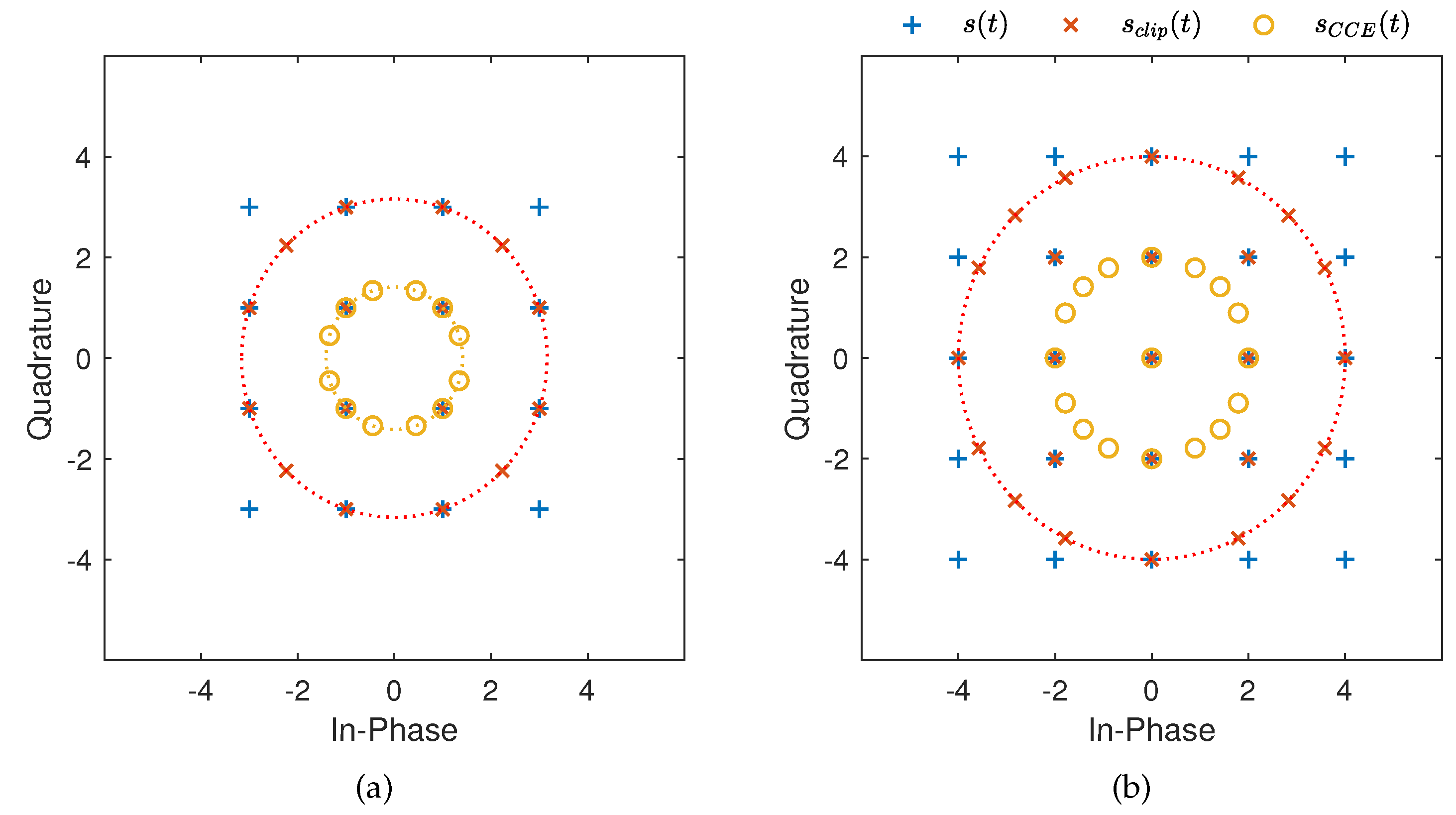
OMBOC(3: 1: 1, 1) and OMBOC(4: 1: 1, 1) are used as examples to demonstrate the performance improvement achieved through clipping. OMBOC(K: 1: 1, 1) consists of K subcarriers, each containing two signal components. The signal components of OMBOC(K: 1: 1, 1) are BOC signals with different subcarrier frequencies, which are evenly distributed across the in-phase and quadrature branches. Figure 1 illustrates the constellations of OMBOC(K: 1: 1, 1) before and after clipping, with the corresponding efficiency improvements presented in Table 2. We observe the following: (1) When the amplitude of the OMBOC signal exceeds the clipping level T, the signal amplitude is compressed by the clipping process without altering the original phase. In contrast, when the amplitude is less than or equal to T, clipping has no effect on the signal. (2) When the clipping level is set to the minimum non-negative amplitude $T_{\min }$, the clipped OMBOC equals the CCE-OMBOC, with all multiplexing signals, except the zero value, located on a circle. To avoid a zero value in OMBOC, it is recommended to set the number of subcarriers to an odd number. (3) The transmission and multiplexing efficiency of OMBOC is significantly enhanced through the clipping process. CCE-OMBOC(3: 1: 1, 1) is a CEM with a transmission efficiency of 1 and a multiplexing efficiency of 84.11%. (4) When the number of subcarriers is even, CCE-OMBOC includes a zero value, resulting in a transmission efficiency less than 1. Except for the zero value, all values of CCE-OMBOC lie in a circle, making it an approximate CEM. For example, CCE-OMBOC(4: 1: 1, 1) contains a zero value, with all other values lying in a circle, resulting in a transmission efficiency of 85.94%.

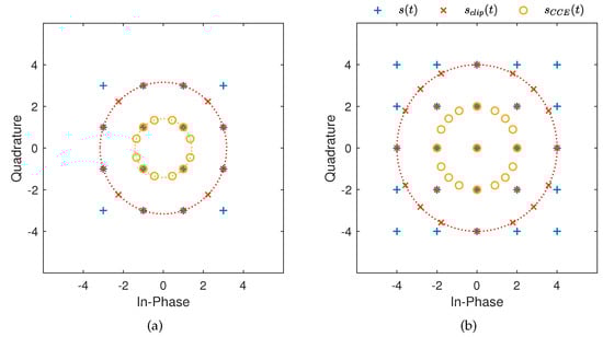
Figure 1. The constellation for original, clipped OMBOC and CCE-OMBOC. (a) OMBOC(3: 1: 1, 1); (b) OMBOC(4: 1: 1, 1).

Table 2. The transmission and multiplexing efficiency before and after clipping.

		Transmission Efficiency ${\mathit{\eta }}_{\mathit{T}}$	Multiplexing Efficiency ηmul	Clipping Level T
OMBOC(3: 1: 1, 1)	Original OMBOC	33.33%	33.33%	/
	Clipped OMBOC	55%	54.41%	$\sqrt{10}$
	CCE-OMBOC	100%	84.11%	$\sqrt{2}$
OMBOC(4: 1: 1, 1)	Original OMBOC	25%	25%	/
	Clipped OMBOC	45.30%	45.00%	4
	CCE-OMBOC	85.94%	76.85%	2

Overall, CCE-OMBOC is a specific form of clipped OMBOC, where the clipping level corresponds to the minimum non-negative amplitude of the original OMBOC. The clipping process significantly enhances the transmission and multiplexing efficiency of OMBOC. The impact of the clipping level on transmission and multiplexing efficiency will be further discussed in the subsequent subsection.

3.2. CCF of CCE-OMBOC

The CCF can be used to describe navigation performance and may be distorted by CEM, indicating that CEM hurts navigation performance. CEM technology is necessary to minimize the potential negative impact, and we find that the CCF of CCE-OMBOC has a fixed ratio which is comparable to that of the original OMBOC. Hence, CCE-OMBOC has a navigation performance that is identical to that of the original OMBOC signal.

The CCF is closely related to the component coefficient vector and can be derived according to the vectorized expression of the clipped OMBOC. The clipped signal value vector ${\mathit{s}}_{\mathrm{clip}}$ can be obtained based on the original OMBOC signal value vector $\mathit{s}$ and clipping level T:

$$s_{\mathrm{clip}}\left[i\right]=\left\{\begin{array}{ccc}\hfill & \tilde{s}\left[i\right]\hfill & \hfill ,|\tilde{s}\left[i\right]|\le T\\ \hfill & T{e}^{j\theta \left(\tilde{s}\left[i\right]\right)}\hfill & \hfill ,|\tilde{s}\left[i\right]|>T\end{array}\right.$$

(15)

where $\tilde{s}\left[i\right]$ (resp. $s_{\mathrm{clip}}\left[i\right]$) is the i-th element of the signal value vector $\mathit{s}$ (resp. clipped signal value vector ${\mathit{s}}_{\mathrm{clip}}$). In addition, ${\mathit{s}}_{\mathrm{clip}}$ can be obtained by adding the original signal value vector $\mathit{s}$ with an intermodulation (IM) value vector $\mathit{\lambda }$ [29], as follows:

$${\mathit{s}}_{\mathrm{clip}}=\mathit{s}+\mathit{\lambda }={\mathit{C}}_0{\mathit{w}}_s^{\prime }+\mathit{\lambda }$$

(16)

where ${\mathit{w}}_s^{\prime }$ denotes the component coefficient vector for the original OMBOC signal in the clipped signal, and the dimension of $\mathit{\lambda }$ is the same as $\mathit{s}$. For the GNSS, the intermodulation (IM) term should not influence the correlation characteristic in the receiver, i.e.,

$${\mathit{c}}_i^{\mathrm{H}}\mathit{\lambda }=0,\forall {\mathit{c}}_i\in {\mathit{C}}_0$$

(17)

Hence, the value subspace of $\mathit{\lambda }$ must be the orthogonal complement of the space expanded by the component value vector ${\mathit{c}}_1,{\mathit{c}}_2,\dots ,{\mathit{c}}_{2K}$, i.e., $\mathit{\lambda }\in {\mathcal{W}}^{\perp }$, where $\mathcal{W}=$ span $\{{\mathit{c}}_1,{\mathit{c}}_2,\dots ,{\mathit{c}}_{2K}\}$. Furthermore, it is easy to verify that ${\mathit{c}}_i$ are orthogonal to each other and can be a basis set for $\mathcal{W}$. It can be proven that dim$\left(\mathcal{W}\right)=2K$ and dim$\left({\mathcal{W}}^{\perp }\right)=F-2K$. A basis set $\mathring{\mathit{C}}$ of ${\mathcal{W}}^{\perp }$ can be constructed from the basis set ${\mathit{c}}_1,{\mathit{c}}_2,\dots ,{\mathit{c}}_{2K}$ [29]:

$$\begin{array}{cc}\hfill \mathring{\mathit{C}}=& \left({\mathring{\mathit{c}}}_1,{\mathring{\mathit{c}}}_2,\dots ,{\mathring{\mathit{c}}}_{F-2K}\right)\hfill \\ \hfill =& (\underset{2\mathrm{nd}\mathrm{IMV}}{\underbrace{{\mathit{v}}^{(1,2)},\cdots ,{\mathit{v}}^{(2K-1,2K)}}},\cdots ,\underset{k\text{-th}\mathrm{IMV}}{\underbrace{{\mathit{v}}^{\left(i_1{i}_2\cdots i_k\right)}}},\hfill \\ \hfill & \cdots ,\underset{2K-\mathrm{th}\mathrm{IMV}}{\underbrace{{\mathit{v}}^{(1,2,\cdots ,2K)}}},\underset{0\mathrm{th}\mathrm{IMV}}{\underbrace{\mathbf{1}}})\hfill \end{array}$$

(18)

where ${\mathring{\mathit{c}}}_i$ is an IM vector (IMV), and ${\mathit{v}}^{(i_1{i}_2\dots i_k)}$ is the Hadamard product (element-wise product) of k specific component value vectors: ${\mathit{c}}_{i_1},{\mathit{c}}_{i_2},\cdots {\mathit{c}}_{i_k}$.

Thus, $\mathit{\lambda }$ can be expressed as a linear combination of elements in its basis set $\left({\mathring{\mathit{c}}}_1,{\mathring{\mathit{c}}}_2,\dots ,{\mathring{\mathit{c}}}_{F-2K}\right)$:

$$\mathit{\lambda }=\left({\mathring{\mathit{c}}}_1,{\mathring{\mathit{c}}}_2,\dots ,{\mathring{\mathit{c}}}_{F-2K}\right){\mathit{w}}_{m,clip}\stackrel{\Delta }{=}\mathring{\mathit{C}}{\mathit{w}}_{m,clip}$$

(19)

where ${\mathit{w}}_{m,clip}={(w_{m,clip}\left(1\right),w_{m,clip}\left(2\right),\dots ,w_{m,clip}(F-2K))}^{\mathrm{T}}\in {\mathbb{C}}^{F-2K}$ is denoted as the IM coefficient vector, and entry $w_{m,clip}\left(i\right)$ corresponds to the weight of ${\mathring{c}}_i$ in $\mathit{\lambda }$.

We define the augmented component value matrix $\mathit{C}=({\mathit{C}}_0,\mathring{\mathit{C}})$ and the augmented coefficient vector $\mathit{w}={({{\mathit{w}}_s^{\prime }}^{\mathrm{T}},{\mathit{w}}_{m,clip}^{\mathrm{T}})}^{\mathrm{T}}$. Substituting (19) into (16), we can obtain a concise form of ${\mathit{s}}_{\mathrm{clip}}$:

$${\mathit{s}}_{\mathrm{clip}}=\mathit{C}\mathit{w}$$

(20)

It can be easily proven that $\mathit{C}{\mathit{C}}^{\mathrm{H}}=F·\mathit{I}$, indicating orthogonality and normalization.

Consequently, the augmented coefficient vector $\mathit{w}$ contains a signal component and IM coefficient vector, and it can be derived by the known clipped signal value vector ${\mathit{s}}_{\mathrm{clip}}$ and augmented component value matrix $\mathit{C}$:

$$\mathit{w}={({{{\mathit{w}}_s}^{\prime }}^{\mathrm{T}},{\mathit{w}}_{m,clip}^{\mathrm{T}})}^{\mathrm{T}}={\displaystyle \frac{1}{F}}{\mathit{C}}^{\mathrm{H}}{\mathit{s}}_{\mathrm{clip}}$$

(21)

OMBOC(3: 1: 1, 1) and OMBOC(4: 1: 1, 1) are used as examples to derive the CCF of the CCE-OMBOC. The component coefficient vector ${\mathit{w}}_s^{\prime }$ plays a crucial role in influencing the CCF of the CCE-OMBOC. The parameters and clipping results are presented in Table 3. ${\mathit{w}}_s^{\prime }$ has the same elements, indicating that each signal component of CCE-OMBOC has equal power. The component coefficient vector ${\mathit{w}}_s^{\prime }$ maintains a fixed ratio $\kappa$ with ${\mathit{w}}_s$:

$${\mathit{w}}_s^{\prime }=\kappa {\mathit{w}}_s$$

(22)

where $\kappa$ is a positive scalar.

Table 3. The parameters and clipping results for the OMBOC.

$({\mathit{\alpha }}_{\mathit{K}}:{\mathit{\alpha }}_{\mathit{d}}:{\mathit{\alpha }}_1,\mathit{\beta })$	$(3:1:1,1)$	$(4:1:1,1)$
Subcarrier number	3	4
Signal component number	6	8
Clipping level	$\sqrt{2}$	2
${\mathit{A}}^{\prime }$	$\sqrt{2}$	2
${\mathit{w}}_s$	${[1,1,1,1j,1j,1j]}^{\mathrm{T}}$	${[1,1,1,1,1j,1j,1j,1j]}^{\mathrm{T}}$
${\mathit{w}}_s^{\prime }$	$0.52951\times {[1,1,1,1j,1j,1j]}^{\mathrm{T}}$	$0.61987\times {[1,1,1,1,1j,1j,1j,1j]}^{\mathrm{T}}$

Then, the CCF of the clipped OMBOC can be derived based on the component coefficient vector. By comparing (9) with (16), the clipped OMBOC can be considered the sum of the original OMBOC signal and IM signal. The IM signal is orthogonal to each signal component in the correlator. There, the correlation between the IM term and the original navigation signal is 0. The correlation $R_{orig,clip}\left(\tau \right)$ between the clipped and original signals depends solely on the component coefficient vector of the clipped signal:

$$R_{orig,clip}\left(\tau \right)=\sum _{i=1}^K\left[\left|w_{s,i}^{\prime }\right|R_{I,i}\left(\tau \right)+\left|w_{s,K+i}^{\prime }\right|R_{Q,i}\left(\tau \right)\right]=\sum _{i=1}^K\kappa \left[R_{I,i}\left(\tau \right)+R_{Q,i}\left(\tau \right)\right]$$

(23)

where $w_{s,i}^{\prime }$ is the i-th element of the clipped component coefficient vector ${\mathit{w}}_s^{\prime }$ and its absolute value $w_{s,i}^{\prime }$ equal to $\kappa$.

Substituting (5) into (23), the CCF of CCE-OMBOC can be derived from the original OMBOC as follows:

$$R_{orig,clip}\left(\tau \right)=\kappa R\left(\tau \right)$$

(24)

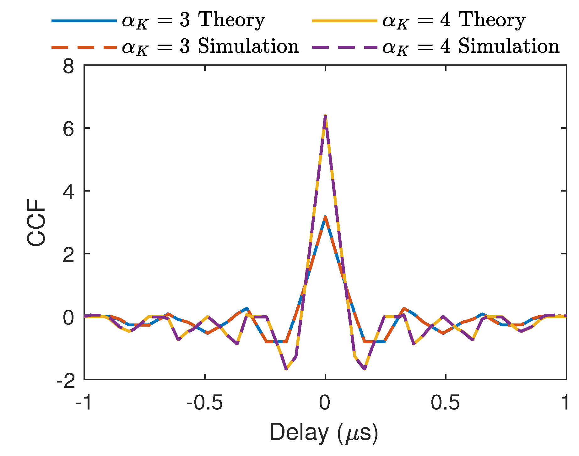
This shows that the CCF of CCE-OMBOC has a fixed ratio $\kappa$, compared to that of the original OMBOC. Therefore, except for the difference in signal power, CCE-OMBOC exhibits navigation performance that is identical to the original OMBOC. To verify the accuracy of (23), we compared the theoretical CCF with the simulated CCF by using CCE-OMBOC(3: 1: 1, 1) and (4: 1: 1, 1). Figure 2 illustrates that the simulated and theoretical correlations are identical.

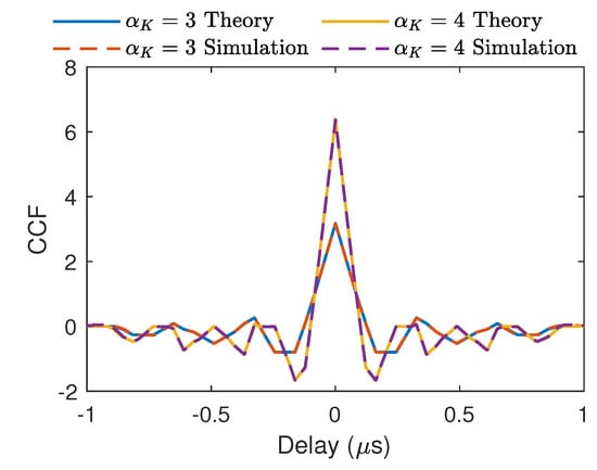
Figure 2. Comparison of the theoretical and simulation correlations $R_{orig,clip}\left(\tau \right)$ of the CCE-OMBOC and original OMBOC$({\alpha }_K:1:1,1)$. The theoretical and simulation results are consistent.

Additionally, the fixed ratio $\kappa$ represents the correlation loss caused by multiplexing in CCE-OMBOC(K: 1: 1, 1), with its value falling within the range (0,1). The correlation loss can be translated into multiplexing efficiency as follows:

$${\eta }_{\mathrm{mul}}={\displaystyle \frac{{\kappa }^2\times 2K}{{\left({\mathit{A}}^{\prime }\right)}^2}}$$

(25)

where $A^{\prime }$ is the maximum amplitude of CCE-OMBOC and equals $T_{\min }$. Even though $\kappa$ is less than 1, CCE-OMBOC significantly enhances multiplexing efficiency compared to OMBOC because the maximum amplitude ${\mathit{A}}^{\prime }$ of CCE-OMBOC also decreases. Moreover, it has been confirmed that the calculation results of ${\eta }_{\mathrm{mul}}$ in (12) and (25) are consistent.

In summary, we first derive the CCF expression of CCE-OMBOC, which maintains a fixed ratio relative to the CCF of OMBOC. Apart from enhancing multiplexing efficiency, CCE-OMBOC retains an identical normalized CCF compared to the original OMBOC, resulting in equivalent navigation performance. Thus, the clipping process of CCE-OMBOC has no unfavorable effect on navigation performance.

3.3. Effect of Clipping Level

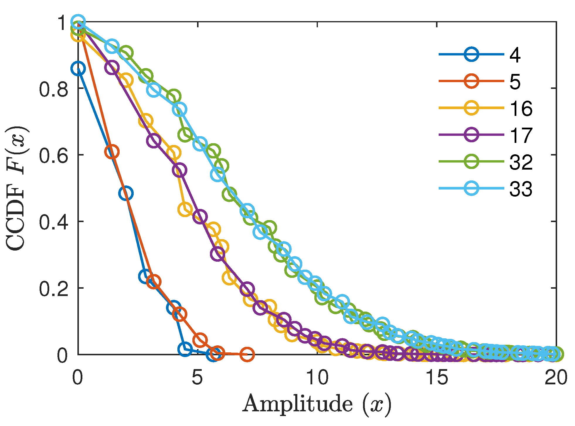
The clipping level significantly impacts the transmission and multiplexing efficiency of the clipped OMBOC, and it can be chosen according to the amplitude distribution of the OMBOC. Indeed, the complementary cumulative distribution function (CCDF) $F\left(x\right)$ is often used to describe the amplitude distribution, and its definition is as follows:

$$F\left(x\right)=Pr(\left|s\left(t\right)\right|>x)=\sum _{V_i>x}{P}_i$$

(26)

where $|·|$ denotes the absolute operator.

The amplitude distribution of OMBOCs with different numbers of subcarriers is shown in Figure 3, and we can draw the following conclusions: (1) For different numbers of subcarriers, the OMBOC has different amplitude distributions. (2) Most of the OMBOC amplitude is less than its maximum amplitude; hence, an enormous amount of power for the transmitter’s HPA is wasted. (3) When the number of subcarriers is odd (resp. even), the minimum non-negative amplitude of the OMBOC is $\sqrt{2}$ (resp. 2).

Figure 3. The amplitude CCDFs of OMBOCs with different numbers of subcarriers.

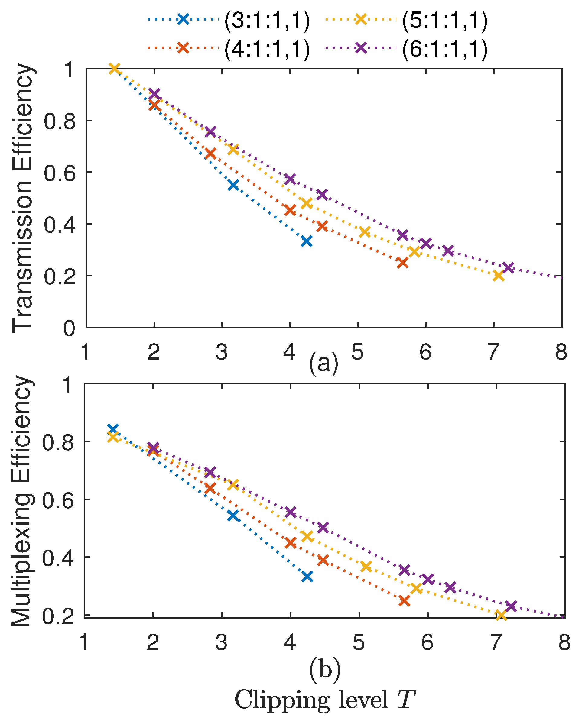
Therefore, the clipping level can be chosen according to the OMBOC amplitude distribution. For different OMBOC signals, the relationship between the transmission efficiency ${\eta }_T$ and multiplexing efficiency ${\eta }_{\mathrm{mul}}$ with different clipping levels T is shown in Figure 4. We make the following observations:

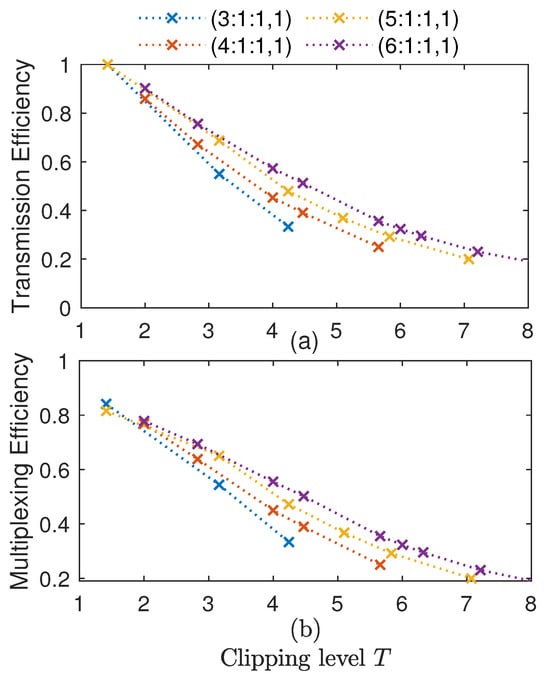
Figure 4. The effect of the clipping level T on the efficiency: (a) transmission efficiency; (b) multiplexing efficiency.

(1) When the number of subcarriers is odd and the clipping level is $T=\sqrt{2}$, ${\eta }_T$ reaches 1. The clipped OMBOC equals CCE-OMBOC and has a constant envelope. (2) On the other hand, when the number of subcarriers is even, the transmission efficiency ${\eta }_T$ of the CCE-OMBOC is greater than $85\%$ but less than 1. The reason is that the original OMBOC’s amplitude vector $\mathit{V}$ has zero elements and the largest ${\eta }_T$ cannot be 1. Thus, the CCE-OMBOC is not a strictly constant envelope due to the zero value. (3) The smaller the clipping level T is, the less power waste there is in the transmitter, leading to higher ${\eta }_T$ and ${\eta }_{\mathrm{mul}}$. Hence, the CCE-OMBOC has the maximum transmission and multiplexing efficiency, relative to other clipped OMBOCs. Moreover, the multiplexing efficiency of CCE-OMBOC is approximately $80\%$.

Hence, the CCE-OMBOC with an odd number of subcarriers has a strictly constant envelope, i.e., ${\eta }_T=1$; in contrast, the CCE-OMBOC with an even number of subcarriers has a zero point, which slightly reduces the transmission efficiency. CCE-OMBOC has a maximum transmission and multiplexing efficiency, relative to other clipped OMBOCs. The multiplexing efficiency of CCE-OMBOC is approximately $80\%$.

4. CCE-OMBOC Performance

Compared with the OMBOC, CCE-OMBOC significantly improves transmission and multiplexing efficiency without sacrificing navigation performance. Additionally, a recommended sampling rate for the CCE-OMBOC is introduced here.

4.1. Transmission and Multiplexing Efficiency Promotion

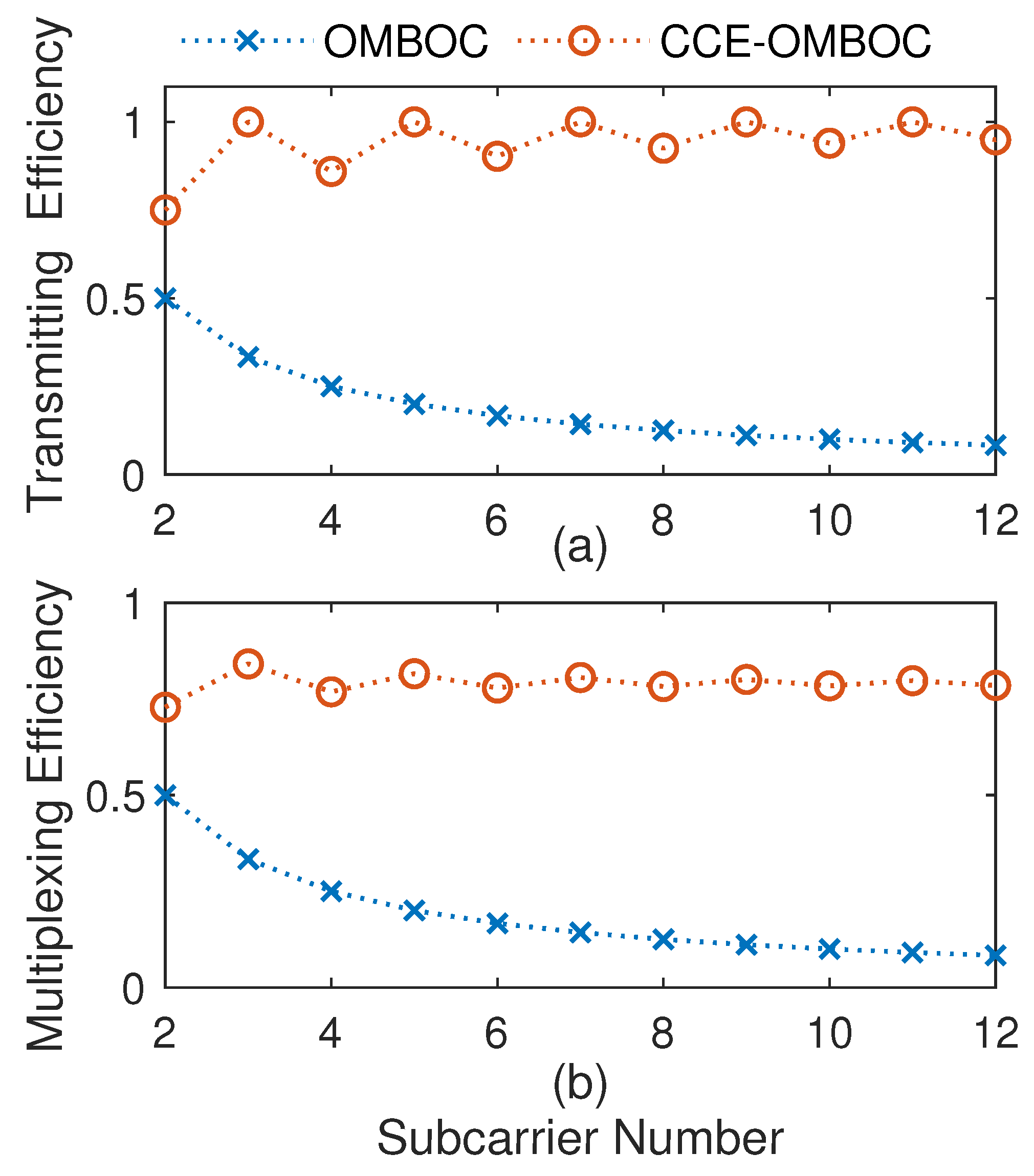
The CCE-OMBOC is proposed to overcome the low transmission and multiplexing efficiency of the OMBOC. An efficiency comparison of the CCE-OMBOC and the original OMBOC for different subcarrier numbers K is shown in Figure 5, and we find that (1) the greater the number of subcarriers is, the lower the transmission and multiplexing efficiency of the OMBOC signal. Compared with the OMBOC, the CCE-OMBOC remarkably enhances the transmission and multiplexing efficiency. (2) The multiplexing efficiency of the CCE-OMBOC fluctuates around $80\%$ for different numbers of subcarriers, indicating that the CCE-OMBOC is an efficient CEM method. For example, when the subcarrier number K equals 3, the multiplexing efficiency of the CCE-OMBOC reaches $84.11\%$, and this modulation contains six navigation signal components. (3) When the number of subcarriers K is even, the transmission efficiency of the CCE-OMBOC is slightly lower than 1 due to the zero value in the signal. However, with the increase in subcarriers, the transmission and multiplexing efficiency tends to stabilize. This is because the probability of zero value decreases with the increasing subcarriers, resulting in minimal impact on the efficiency. The stable multiplexing efficiency of CCE-OMBOC is approximately 80%.

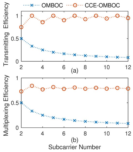
Figure 5. CCE-OMBOC enhances the efficiency for any number of subcarriers: (a) Transmission efficiency; (b) Multiplexing efficiency.

In general, the CCE-OMBOC notably enhances the transmission and multiplexing efficiency of the OMBOC (from below $50\%$ to approximately $80\%$).

4.2. Suggested Sampling Rate

The sampling rate $f_s$ is closely related to the CCE-OMBOC parameter $({\alpha }_K:{\alpha }_d:{\alpha }_1,\beta )$ and is the key parameter in the navigation system. The navigation modulation is expected to reduce the sampling rate as much as possible while guaranteeing navigation performance. As a square wave is used in the subcarrier, generating the CCE-OMBOC and OMBOC becomes straightforward, making the sampling rate requirement relatively low.

When the subcarriers are sinusoidal signals, the sampling rate increases significantly with increasing subcarriers for multicarrier CEM. For example, a multicarrier signal has K subcarriers that are located at $\{1,2,\cdots ,K\}{f}_0$. Each subcarrier has four sampling points in a period, and the sampling hold time is $\Delta t_i=1/\left(4i{f}_0\right)$ for subcarrier i [38]. To ensure integrity in the CEM optimization, the sampling interval ($t_s=1/f_s$) should be the least common divisor of all subcarrier waveform hold times $\Delta t_i$. The sampling rate with 5 (resp. 10) subcarriers is $240f_0$ (resp. 10,080$f_0$). The high sampling rate results in the high cost of receivers.

The sampling rate of the CCE-OMBOC is suggested to be $4{\alpha }_K{f}_0$. According to the signal model, it is clear that the subcarrier of the CCE-OMBOC is a square wave. In a subcarrier period, each subcarrier has four phase-shifting time points and requires at least four sampling points. Although the CCE-OMBOC has K subcarriers, the Kth subcarrier of the CCE-OMBOC plays a noteworthy role in tracking accuracy [11]. Moreover, $4{\alpha }_K{f}_0$ is higher than the required sampling rates of the other subcarriers. Hence, the minimum sampling rate ($4{\alpha }_K{f}_0$) of subcarrier K is suggested as the CCE-OMBOC sampling rate.

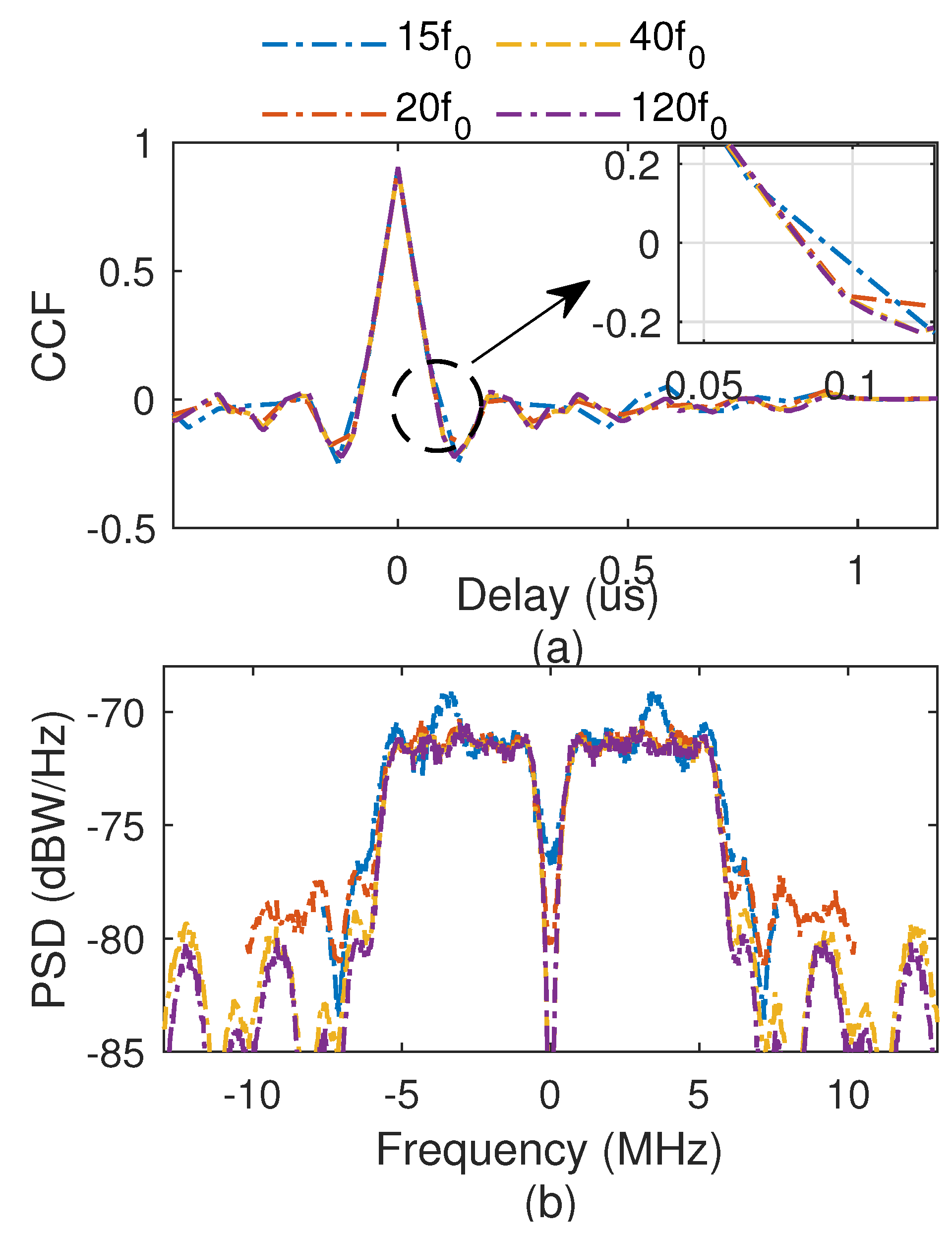
To analyze the effect of the sampling rate on the CCF and power spectral density (PSD), four different sampling rates are used for CCE-OMBOC(5: 1: 1, 1), and the comparison results are shown in Figure 6. We find that (1) when the sampling rate is equal to or greater than $4{\alpha }_K{f}_0=20f_0$, the main peaks of the CCF and main lobes of PSD are similar, indicating they have similar navigation performance. Hence, $4{\alpha }_K{f}_0$ is a sufficient sampling rate for the expected tracking accuracy. (2) When the sampling rate is less than $4{\alpha }_K{f}_0$, the main bandwidth of the CCF is larger than the expected main bandwidth, and the main lobe of PSD differs from others, indicating tracking performance decreases. In conclusion, $4{\alpha }_K{f}_0$ is the proper sampling rate for CCE-OMBOC modulation.

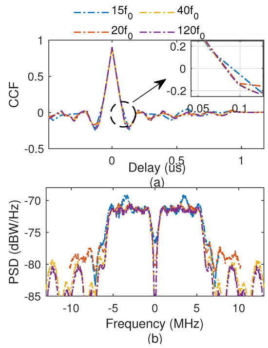
Figure 6. Effect of the sampling rate: (a) CCF; (b) PSD.

5. Advantages of CCE-OMBOC over Traditional CEM Methods

The CCE-OMBOC was compared with several representative CEM methods: CEMIC [29], ACE-FHBOC [28] and MV [15]. The results show that the proposed CCE-OMBOC is an efficient CEM multiplexing method. Additionally, because the CCE-OMBOC subcarriers have different frequencies, the CCE-OMBOC has high tracking accuracy and excellent compatibility.

5.1. Comparing the CCE-OMBOC with CEMIC

The comparison between CCE-OMBOC and CEMIC reveals that they share the same multiplexing efficiency, indicating that CCE-OMBOC serves as an equivalent solution to CEMIC for OMBOC. However, the process of generating CCE-OMBOC is significantly simpler than that of CEMIC. CEMIC is an optimal solution for a constrained multiplexing problem that provides minimum energy of the IM term [29,39].

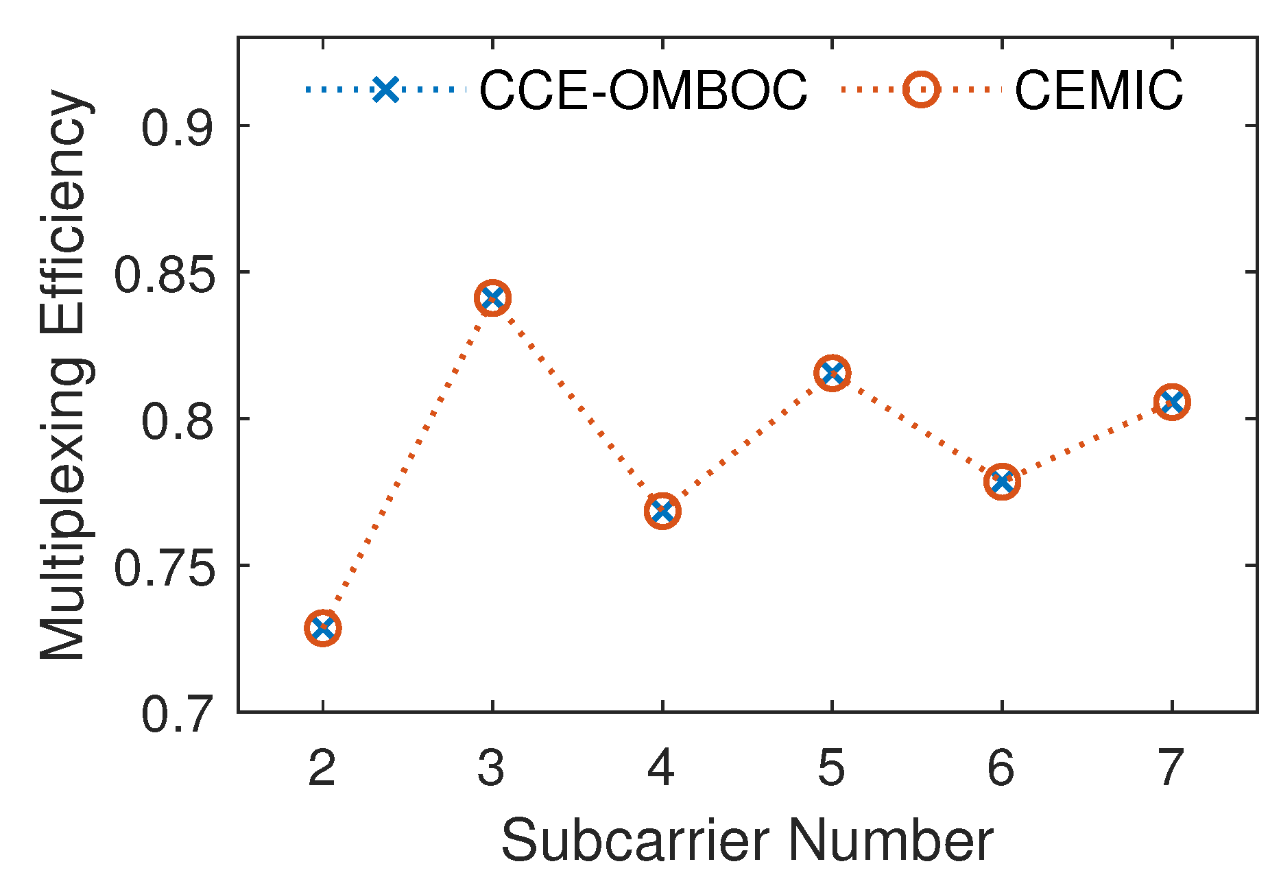
We first compare the multiplexing efficiency of CCE-OMBOC and CEMIC for different subcarrier numbers of OMBOC. As the number of subcarriers increases, the transmission and multiplexing efficiencies of OMBOC gradually decrease. CCE-OMBOC and CEMIC can be used to overcome the low efficiency of the OMBOC. The number of OMBOC subcarriers (resp. signal components) in the comparison is $\{2,3,\cdots ,7\}$ (resp. $\{4,6,\cdots ,14\}$). The comparison results of the multiplexing efficiency are shown in Figure 7. The CCE-OMBOC has a multiplexing efficiency identical to that of CEMIC, indicating that the CCE-OMBOC can achieve optimal multiplexing efficiency.

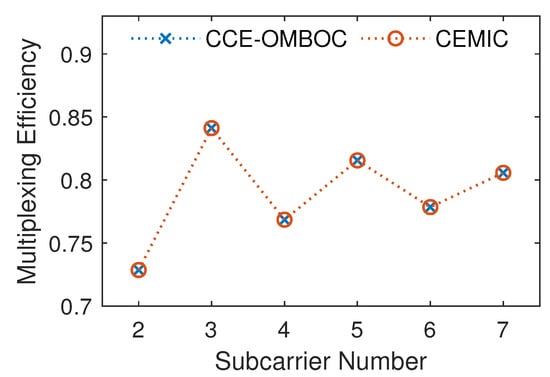
Figure 7. Comparison of multiplexing efficiency for different numbers of subcarriers.

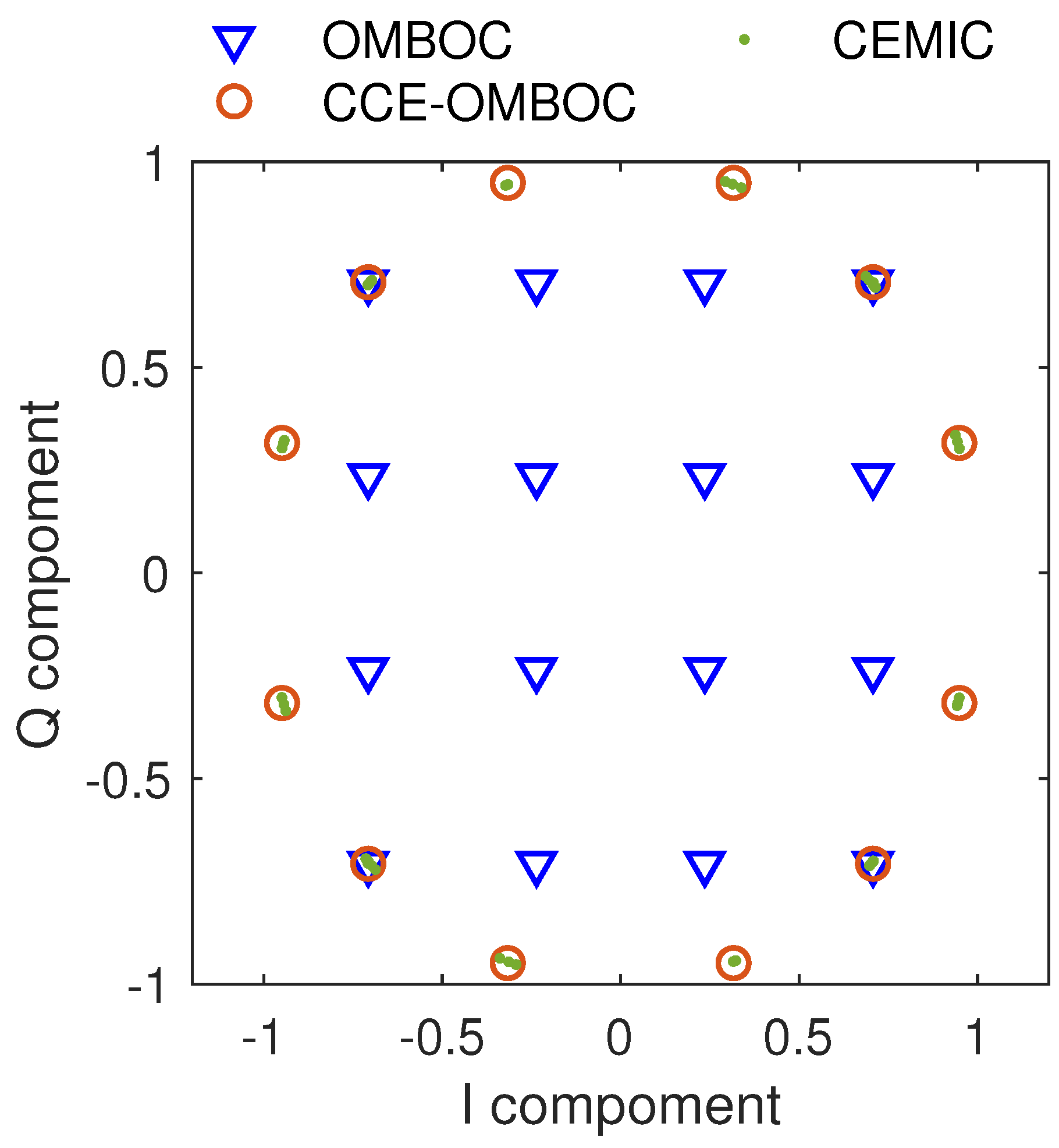
Next, the constellation is used to analyze the difference between the CCE-OMBOC and CEMIC, as shown in Figure 8 and Table 4. The OMBOC(3: 1: 1, 1) is used in the comparison, and it is easy to generate the CCE-OMBOC based on the original signal by clipping. CEMIC is an optimization algorithm, and the initial value of the optimization coefficient is set as a zero vector. For OMBOC(3: 1: 1, 1), there are six signal components, and the optimization coefficient vector ${\mathit{w}}_{m,opt}$ in CEMIC has 58 elements. We found that the CCE-OMBOC has a similar constellation and multiplexing efficiency to CEMIC, indicating that CCE-OMBOC is equivalent to CEMIC for the OMBOC. Moreover, the slightly lower ${\eta }_{\mathrm{mul}}$ of CEMIC (83.50%) compared to CCE-OMBOC(84.10%) may be due to the stopping conditions of the CEMIC iterations, which prevent the algorithm from reaching its absolute optimal ${\eta }_{\mathrm{mul}}$. This result also highlights the trade-off between optimization complexity and performance in CEMIC.

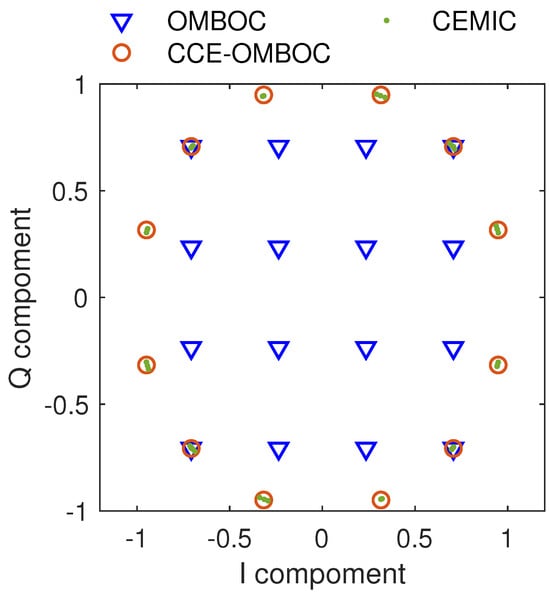
Figure 8. Comparison of amplitude-normalized constellations for different modulations: original OMBOC, CCE-OMBOC, and CEMIC.

Table 4. Comparison of the CCE-OMBOC with CEMIC for OMBOC(3: 1: 1, 1).

	OMBOC	CCE-OMBOC	CEMIC
${\mathit{w}}_s$	${[1,1,1,1j,1j,1j]}^{\mathrm{T}}$	${[1,1,1,1j,1j,1j]}^{\mathrm{T}}$	${[1,1,1,1j,1j,1j]}^{\mathrm{T}}$
Initial ${\mathit{w}}_m$	\	\	$\overrightarrow{0}$
${\eta }_T$	33.33%	100%	100%
${\eta }_{\mathrm{mul}}$	33.33%	84.10%	83.50%

According to the comparison of constellation and multiplexing, CCE-OMBOC has identical multiplexing efficiency and constellation to CEMIC for OMBOC signals. Hence, CCE-OMBOC is equivalent to the optimization method of CEMIC for the OMBOC signal. Due to CEMIC providing maximum multiplexing efficiency, CCE-OMBOC can be considered to provide optimal multiplexing efficiency.

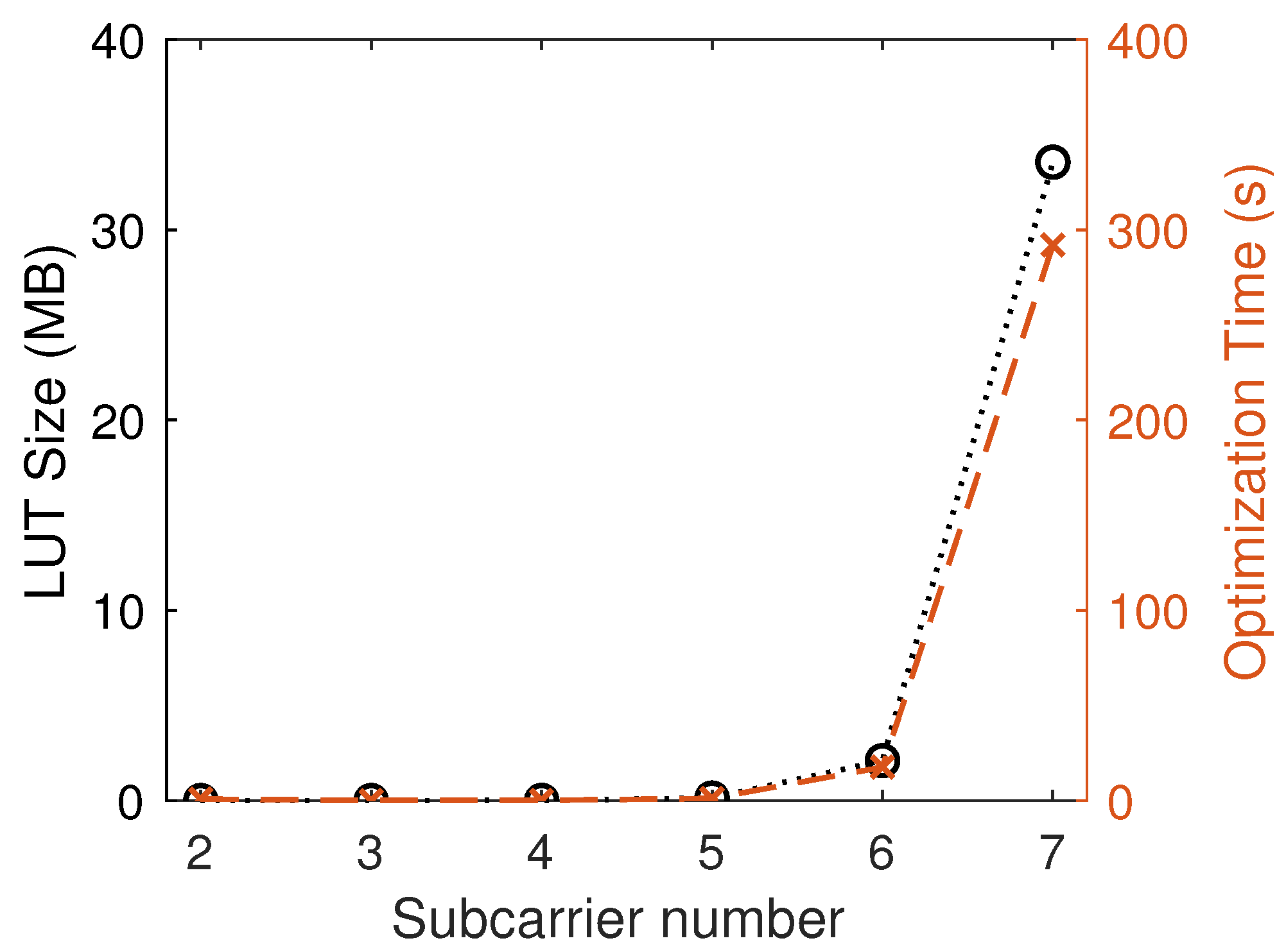
Furthermore, upon comparing the generation complexity, the generation process of CCE-OMBOC is significantly simpler than that of CEMIC. For CCE-OMBOC, the procedure merely adds a clipping step to the original OMBOC generation, making it relatively straightforward. In contrast, the CEMIC approach becomes increasingly complex as the number of subcarriers grows. (1) Lookup Table Size: As the number of subcarriers increases, the size of the lookup table (LUT) for CEMIC expands exponentially (as shown in Figure 9), leading to inefficiencies and higher costs. (2) Optimization Time: Figure 9 also illustrates a sharp rise in optimization time with the growing number of subcarriers. This increase is due to the fact that CEMIC’s optimization focuses on the coefficients of IM components, and more subcarriers mean more IM components, resulting in more optimization time and complexity. (3) Initial Vector and Iteration Direction: The selection of an initial vector and the direction of iteration are critical factors that significantly impact the optimization results [39]. For example, OMBOC(10: 1: 1, 1) has $2^{20}-20$ optimization coefficients, and choosing an initial vector becomes increasingly complex. In summary, while the complexity of CEMIC may not be a major concern for fixed systems with a one-time setup, it becomes a critical factor in dynamic reconfigurable systems, such as integrated communication and navigation.

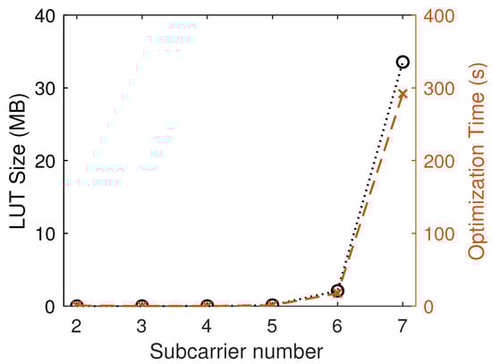
Figure 9. The LUT size and optimization time with different numbers of subcarriers.

5.2. Comparison of CCE-OMBOC with MV and ACE-FHBOC

This subsection compares CCE-OMBOC with MV and ACE-FHBOC to demonstrate that CCE-OMBOC has an advantage because the subcarrier is located at different frequencies. CCE-OMBOC can be viewed as an extension of MV and ACE-FHBOC. The comparison results show its superior tracking performance, compatibility, and efficient generation process, driven by its multicarrier signal model. MV is a CEM multiplexing method designed for single-carrier signals [15]. Compared to MV, the subcarriers of CCE-FHBOC are spectrum-split by the BOC signal and placed in the Q branch. ACE-FHBOC is a frequency-hopping CEM multiplexing method for multicarrier systems [28]. Compared to ACE-FHBOC, the subcarriers of CCE-FHBOC hold all the time slots.

For a fair comparison, signal components of the listed signals have the same code rate $f_0$ and equal power allocation. CCE-OMBOC(3: 1: 1, 1), which has three subcarriers, is used in comparison. ACE-FHBOC has the same main lobe bandwidth as CCE-OMBOC, and its subcarrier hops with time. Since the Q branch in the MV scheme is typically used for unequal power multiplexing [15], only the I branch is considered in the comparison for equal-power CEM. Similar to CCE-OMBOC, the I branch in MV contains three signal components. The detailed parameters of the listed CEM signals are provided in Table 5.

Table 5. The parameters of the CCE-OMBOC, ACE-FHBOC and MV.

Modulation Type	CCE-OMBOC	ACE-FHBOC	MV
Number of Subcarriers	3	3	1
Original ${\eta }_T$	33.3%	50%	33.3%
${\eta }_T$	100%	100%	100%
${\eta }_{\mathrm{mul}}$	84.11%	85.36%	75%
ZCNM (ns)	127	127	980
MLB (MHz)	8.18	8.18	2.05
MVP (dBW/Hz)	−68.67	−68.67	−60.09

MV has an odd number of signal components and makes up the majority of the input signals.

$$s_{MV}=\mathrm{sign}\left(s_1+s_2+s_3\right)$$

(27)

These three components $s_i$ are independent of each other.

Additionally, compared with the original composite signals, all the listed CEM methods construct a constant-envelope signal and significantly enhance the transmission efficiency (shown in Table 5). Because the MV does not contain a quadrature branch, the multiplexing efficiency of the MV is lower than that of the CCE-OMBOC.

5.2.1. Tracking Performance

The tracking performance is the most important indicator for navigation modulation and can be evaluated by its time-frequency characteristics, CCF and PSD. Moreover, some time-frequency parameters can be calculated from the CCF and PSD for quantitative analysis of the tracking performance [37]:

• Zero-crossing point nearest to the main peak of the CCF (ZCNM). The smaller the ZCNM, the more accurate the code track loop for the navigation signal.

  $${\tau }_{ZCNM}=\underset{\tau >0}{argmin}\left|R\right(\tau \left)\right|$$

  (28)
• Main lobe bandwidth of the PSD (MLB). This affects the power distribution of the main lobe, and the bandwidth of the receiver must be greater than the MLB.
• Maximum value of the PSD (MVP) [10]. This reflects the anti-inference ability, which is detrimental to the tracking accuracy. The smaller the MVP, the stronger the anti-inference ability.

  $$MVP=maxS\left(f\right)$$

  (29)

  where $S\left(f\right)$ is the normalized PSD of the navigation signal.

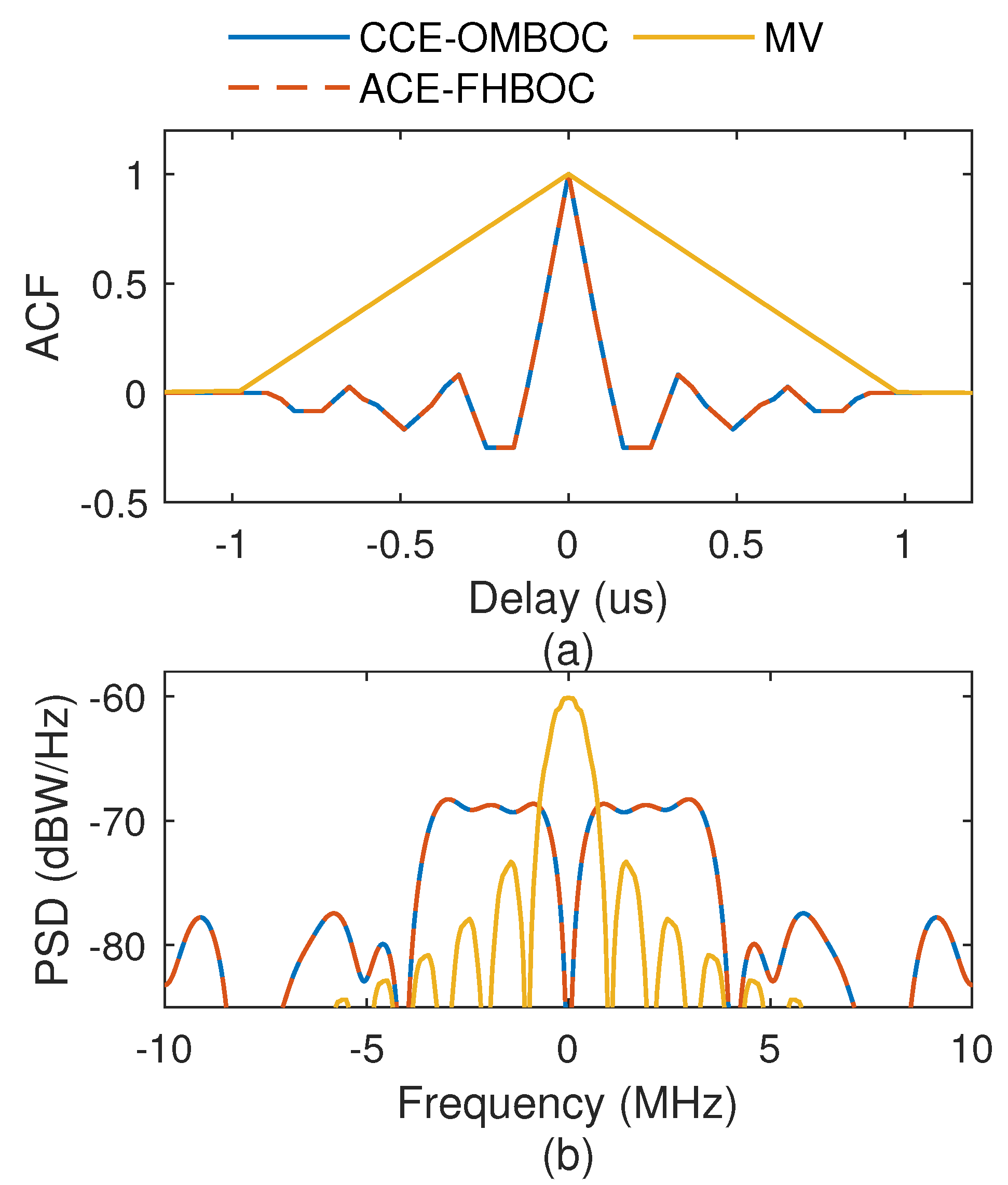
We compare the time-frequency properties of the CCE-OMBOC with those of the MV and ACE-FHBOC, and the results are shown in Figure 10 and Table 5. (1) The CCF of the CCE-OMBOC exhibits an impressive ZCNM at 83 ns, which is much smaller than the ZCNM of the MV (980 ns). This indicates that the CCE-OMBOC has a higher tracking accuracy than the MV because the subcarriers of the CCE-OMBOC are at different frequencies and can enhance the tracking performance. (2) The CCE-OMBOC has a CCF and PSD identical to those of the ACE-FHBOC, which means that they have the same tracking performance. For the ACE-FHBOC, the subcarrier frequency hops with time; in contrast, the subcarriers of the CCE-OMBOC are constant. (3) The CCE-OMBOC has a flat main lobe with PSD and low MVP (−68.67). This indicates that the CCE-OMBOC has a strong anti-inference ability and is efficient for the frequency spectrum.

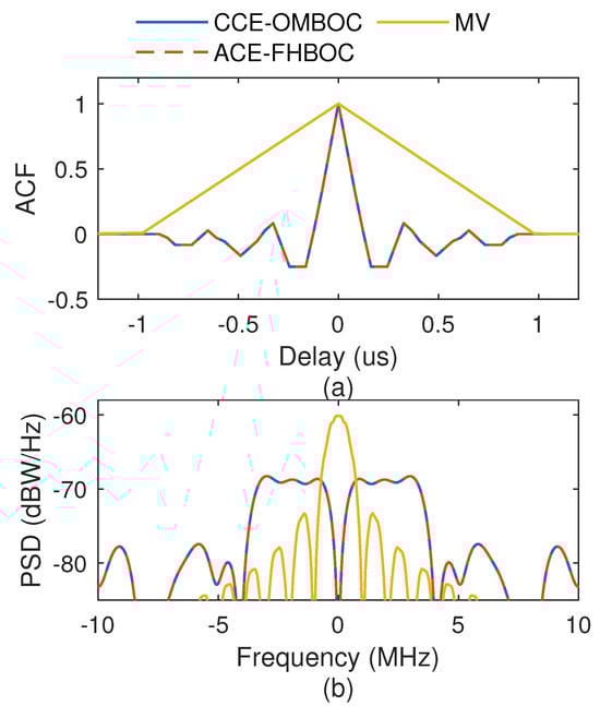
Figure 10. Comparison of different modulations. (a) Normalized CCFs. (b) Normalized PSDs.

In general, because the subcarriers are located at different frequencies, the CCE-OMBOC has better tracking performance than the single-carrier CEM MV.

5.2.2. Compatibility

To accommodate different navigation scenarios and requirements, navigation modulation should have good compatibility. Two key factors, the unmatched reception and spectral separation coefficient (SSC), are used to evaluate the compatibility of the navigation signal. The receiver operates in unmatched reception when the receiver replica signal only contains part of the navigation signal waveform. With an increase in CCE-OMBOC subcarriers, the previous receiver works in unmatched reception, hence the CCE-OMBOC has good compatibility with navigation system upgrades. The receiver operates in unmatched reception when the receiver replica signal only contains part of the navigation signal waveform, which is important for GNSS upgrades. The SSC reflects interference, and a low SSC means less interference between different signals. Its definition is as follows:

$$SSC={\int }_{-\infty }^{+\infty }{S}_1\left(f\right)S_2\left(f\right)df$$

(30)

where $S_i\left(f\right)$ is the normalized PSD for navigation signal i.

First, the compatibility of the ACE-FHBOC is poor due to its strict requirements for matching modulation parameters between the receivers and transmitter, which limits its operation in unmatched reception scenarios. For example, when the ACE-FHBOC adds a new subcarrier, the frequency-hopping pattern changes, and the original receivers cannot work. Additionally, the four signal components of the ACE-FHBOC, which are distributed in the dual-frequency and I/Q branches, exhibit minimal interference with each other, leading to a negligible SSC.

Next, the SSC comparison of the CCE-OMBOC and MV is discussed, and the SSC is calculated according to the subcarrier of the CEM signal. For CCE-OMBOC, the SSC is calculated by the adjacent subcarriers; due to the signal components of MV located in a single carrier, its SSC is calculated by two signal components. The SSC of the MV is −67.77 dB, which is greater than that of the CCE-OMBOC(−78.87 dB), as shown in Table 6, indicating that the MV has greater interference than CCE-OMBOC. This is because all the signal components of the MV are located on a single carrier. In contrast, the subcarriers of the CCE-OMBOC are distributed at adjacent frequency points, which achieves a good balance between the spectral efficiency and the SSC of the subcarriers. Hence, the CCE-OMBOC has an outstanding SSC value, which enhances its compatibility.

Table 6. Comparison of multicarrier constant-envelope modulations regarding compatibility and generation complexity.

Modulation Type	CCE-OMBOC	ACE-FHBOC	MV
SSC	−78.87	/	−67.77
Interference	Little	No	Strong
Unmatched Reception	Excellent	/	General
Compatibility	Excellent	Poor	Middle
Sampling Rate	12$f_0$	24$f_0$	2$f_0$
Generation Complexity	Simple	Complex	Simple

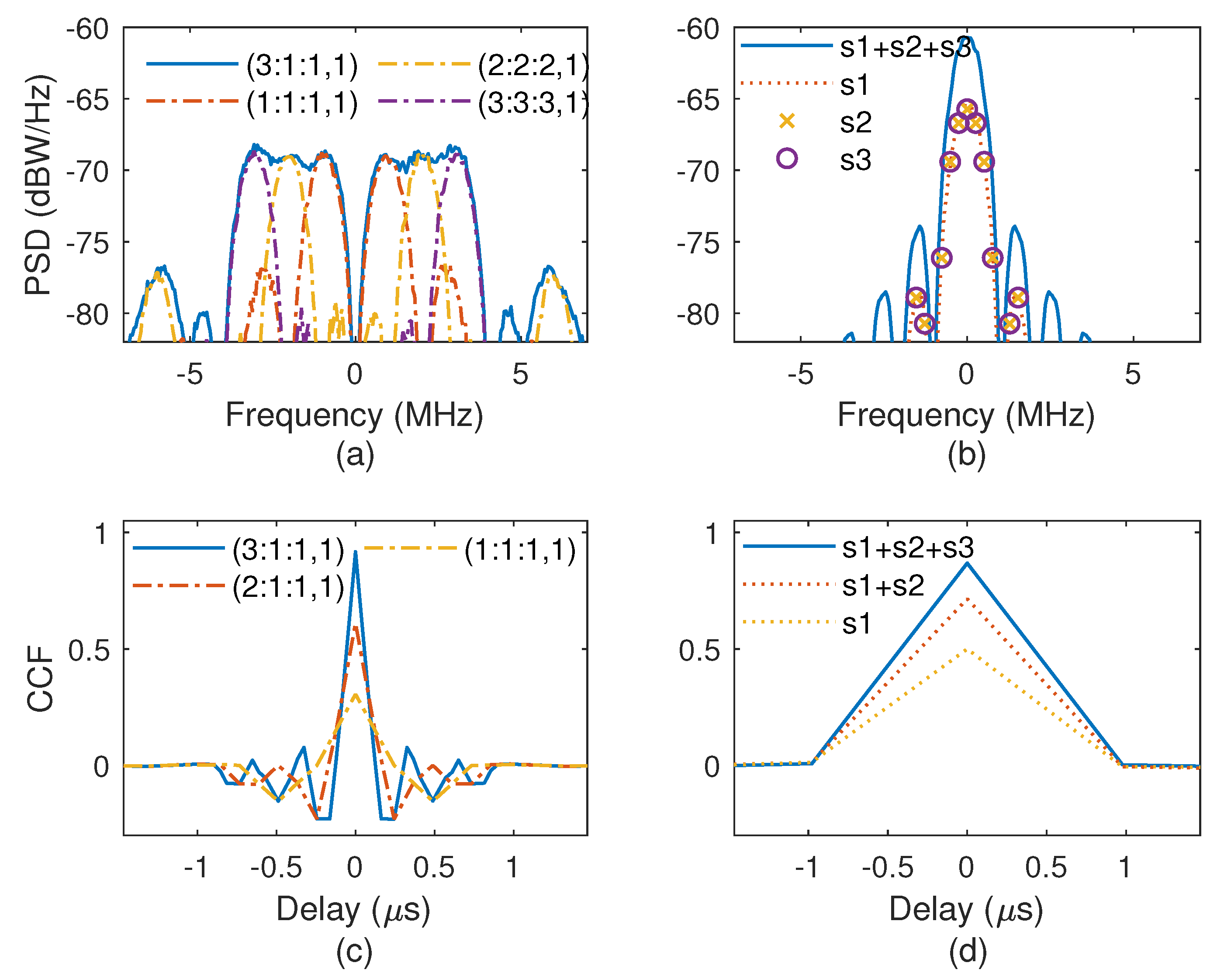
The PSD and CCF comparisons of unmatched reception for the CCE-OMBOC and MV are shown in Figure 11. The subcarrier PSDs of the CCE-OMBOC are located at different frequencies, and these subcarriers exhibit excellent spectrum isolation, which results in a low SSC for the CCE-OMBOC. Moreover, the CCE-OMBOC subcarriers have adjacent frequencies, which enhances the frequency efficiency. In contrast, the PSDs of the MV subcarriers are located in a single carrier, and the subcarriers strongly interfere with each other.

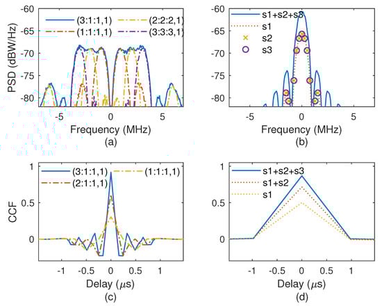
Figure 11. The time-frequency characteristics of the CCE-OMBOC and MV for unmatched reception. (a) PSD of the CCE-OMBOC and its subcarrier. (b) PSD of the MV and its subcarrier. (c) The CCF of the CCE-OMBOC and its subcarrier. (d) The CCF of MV and its subcarrier.

Moreover, the tracking performance of unmatched reception can be analyzed according to the CCF of the CEM signal with its subcarrier. For the CCE-OMBOC, the ZCNMs have different values with different replica subcarriers, indicating that CCE-OMBOC receivers can operate with different tracking accuracies for various navigation requirements. Therefore, the CCE-OMBOC has diverse reception strategies and can obtain flexibly upgraded navigation signals without changing the receiver, which is meaningful for next-generation GNSS and integrated communication and navigation. For different subcarrier combinations, the ZCNM of the MV is the same, and the MV has identical tracking accuracy for unmatched reception.

In conclusion, the CCE-OMBOC has excellent compatibility compared to the MV and ACE-FHBOC because the subcarriers are located at different frequencies. It exhibits low subcarrier SSC and flexible unmatched reception.

5.2.3. Generation Complexity and Signal Components

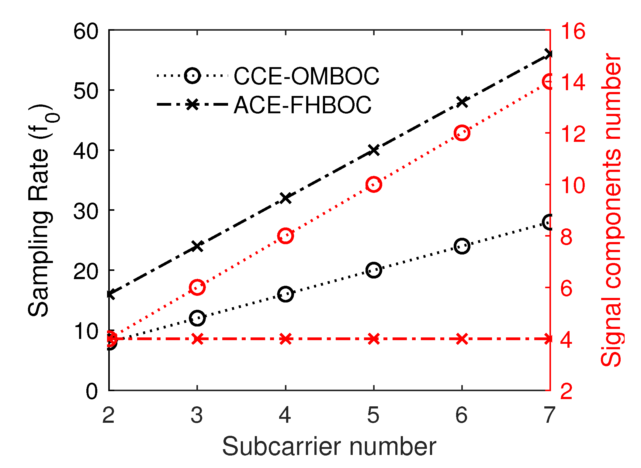
For the GNSS, the generation complexity of the navigation signal is closely related to the cost of the receiver and is significantly impacted by the sampling rate. MV is a CEM technology in single-carrier mode, and the sampling rate is fixed for any signal components. For CCE-OMBOC and ACE-FHBOC, the relationship between the sampling rate and subcarrier number is shown in Figure 12. The CEM construction of the ACE-FHBOC requires at least eight sampling points for every subcarrier period. When the signal has K subcarriers, the required sampling rate of the CCE-OMBOC(resp. ACE-FHBOC) is $4K{f}_0$ (resp. $8K{f}_0$), and the sampling rate of the CCE-OMBOC is less than that of the ACE-FHBOC. Hence, the generation cost of the ACE-FHBOC is greater than that of the CCE-OMBOC, and the generation process of the CCE-OMBOC is simpler than that of the ACF-FHBOC.

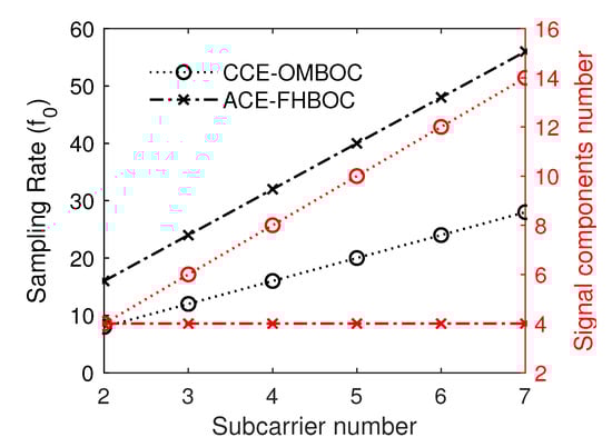
Figure 12. The sampling rate and number of signal components vary with the number of subcarriers.

Additionally, the more signal components, the more navigation services, or the higher the navigation data rate. The signal components of the CCE-OMBOC increase with an increasing number of subcarriers, but ACE-FHBOC has only four signal components for any number of subcarriers.

In conclusion, the comparison results demonstrate that CCE-OMBOC has good tracking performance, compatibility, and simple generation due to its subcarriers located at adjacent frequencies.

6. Conclusions

Based on the clipping method, this paper presents a multicarrier CEM technology called the CCE-OMBOC to address the low efficiency of multicarrier navigation signals. We analyzed the function of the clipping level and found that the CCE-OMBOC has better transmission and multiplexing efficiency than other clipped OMBOCs. According to the derived analytical CCF of the clipped OMBOC, the clipping process does not adversely affect navigation performance. We presented the expression of the transmission and multiplexing efficiency and found that the greater the number of subcarriers, the lower the transmission and multiplexing efficiency. The CCE-OMBOC significantly enhances these efficiencies. A proper sampling rate for the CCE-OMBOC is also suggested for its generation system.

The CCE-OMBOC has been compared with several traditional navigation modulation methods. Compared with CEMIC, the CCE-OMBOC has optimal multiplexing efficiency and a simple generation process. Compared with the MV and ACE-FHBOC, the CCE-OMBOC has high tracking accuracy, excellent compatibility, and a low sampling rate. Hence, the CCE-OMBOC is a promising multicarrier broadband navigation modulation method for next-generation GNSS. Due to its flexible bandwidth, it can also be used to integrate communication and navigation.

Based on the CCE-OMBOC, future works will explore CEM methods with arbitrary power allocations for subcarriers and reception strategies for multicarrier navigation signals.

Appendix A.1. CCF for OMBOC Signal Components

The signal components of the OMBOC are orthogonal, and the complete theoretical derivation is shown in [11]. The CCF $R_{I,i}\left(\tau \right)$ for OMBOC subcarrier i in the in-phase is expressed as follows:

$$\begin{array}{cc}\hfill & R_{I,i}\left(\tau \right)={\displaystyle \frac{T_{S,i}}{2T_C}}\sum _{n=0}^{2n_i-1}{\sum _{m=0}^{2n_i-1}\left(-1\right)}^{m+n+⌊{\displaystyle \frac{m}{2}}⌋+⌊{\displaystyle \frac{n}{2}}⌋}\hfill \\ \hfill & \times {\Lambda }_{T_{S,i}/2}\left(\tau -\left(m+n+1-2n_i\right){\displaystyle \frac{T_{S,i}}{2}}\right)\hfill \end{array}$$

(A1)

where $T_{S,i}=0.5{\left(f_{S,i}\right)}^{-1}$ is the period of subcarrier i, $n_i={\alpha }_i/\beta$, and ${\Lambda }_{T_{S,i}}$ is the triangle function with parameter $T_{S,i}$:

$${\Lambda }_{T_{S,i}}\left(\tau \right)=\left\{\begin{array}{ccc}\hfill & 1-{\displaystyle \frac{\left|\tau \right|}{T_{S,i}}},\hfill & \hfill \left|\tau \right|<T_{S,i}\\ \hfill & 0,\hfill & \hfill \mathrm{otherwise}\end{array}\right.$$

(A2)

Similarly, the CCF $R_{Q,i}\left(\tau \right)$ for OMBOC subcarrier i in quadrature is expressed as follows:

$$\begin{array}{cc}\hfill & R_{Q,i}\left(\tau \right)={\displaystyle \frac{T_{S,i}}{T_C}}\sum _{n=0}^{n_i-1}{\sum _{m=0}^{n_i-1}\left(-1\right)}^{m+n+1}\hfill \\ \hfill & \times {\Lambda }_{T_{S,i}}\left(\tau -\left(m+n+1-n_i\right)T_{S,i}\right)\hfill \end{array}$$

(A3)

References

- Yao, Z.; Lu, M. Next-Generation GNSS Signal Design: Theories, Principles and Technologies; Springer: Berlin/Heidelberg, Germany, 2021. [Google Scholar]
- Zhang, R.; Li, K.; Wu, Y.; Zhao, D.; Lv, Z.; Li, F.; Chen, X.; Qiu, Z.; Yu, F. A Multi-Vehicle Longitudinal Trajectory Collision Avoidance Strategy Using AEBS with Vehicle-Infrastructure Communication. IEEE Trans. Veh. Technol. 2022, 71, 1253–1266. [Google Scholar] [CrossRef]
- Paden, B.; Cap, M.; Yong, S.Z.; Yershov, D.; Frazzoli, E. A Survey of Motion Planning and Control Techniques for Self-driving Urban Vehicles. IEEE Trans. Intell. Veh. 2016, 1, 33–55. [Google Scholar] [CrossRef]
- Khalife, J.; Kassas, Z.M. On the Achievability of Submeter-Accurate UAV Navigation with Cellular Signals Exploiting Loose Network Synchronization. IEEE Trans. Aerosp. Electron. Syst. 2022, 58, 4261–4278. [Google Scholar] [CrossRef]
- Liu, X.; Liang, M.; Morton, Y.; Closas, P.; Zhang, T.; Hong, Z. Performance evaluation of MSK and OFDM modulations for future GNSS signals. GPS Solut. 2014, 18, 163–175. [Google Scholar] [CrossRef]
- Luo, R.; Xu, Y.; Yuan, H. Performance Evaluation of the New Compound-Carrier-Modulated Signal for Future Navigation Signals. Sensors 2016, 16, 142. [Google Scholar] [CrossRef]
- Zhao, X.; Huang, X.; Liu, Z.; Xiao, Z.; Sun, G. Improved MBOC modulations based on periodic offset subcarrier. IET Commun. 2021, 15, 1831–1848. [Google Scholar] [CrossRef]
- Nunes, F.D.; Sousa, F.M.; Leitão, J.M. Characterization and performance analysis of generalized BOC modulations for GNSS. Navigation 2019, 66, 185–197. [Google Scholar] [CrossRef]
- Kong, S.H.; Cho, S.; Kim, T.; Lee, S. Stepped-Frequency Binary Offset Carrier Modulation for Global Navigation Satellite Systems. IEEE Trans. Aerosp. Electron. Syst. 2023, 59, 2733–2751. [Google Scholar] [CrossRef]
- Ma, J.; Yang, Y.; Li, H.; Li, J. FH-BOC: Generalized low-ambiguity anti-interference spread spectrum modulation based on frequency-hopping binary offset carrier. GPS Solut. 2020, 24, 70. [Google Scholar] [CrossRef]
- Deng, L.; Yang, Y.; Ma, J.; Feng, Y.; Ye, L.; Li, H. OFDM-BOC: A Broadband Multicarrier Navigation Modulation-Based BOC for Future GNSS. IEEE Trans. Veh. Technol. 2024, 73, 3964–3979. [Google Scholar] [CrossRef]
- Han, S.H.; Lee, J.H. An overview of peak-to-average power ratio reduction techniques for multicarrier transmission. IEEE Wirel. Commun. 2005, 12, 56–65. [Google Scholar] [CrossRef]
- Li, X.; Cimini, L.J. Effects of clipping and filtering on the performance of OFDM. IEEE Commun. Lett. 1998, 2, 131–133. [Google Scholar]
- Kaplan, E.D.; Hegarty, C. Understanding GPS: Principles and Applications, 2nd ed.; Artech House Publishers: Norwood, MA, USA, 2005. [Google Scholar]
- Spilker, J.J.; Orr, R.S. Code Multiplexing via Majority Logic for GPS Modernization. In Proceedings of the 11th International Technical Meeting of the Satellite Division of The Institute of Navigation (ION GPS 1998), Nashville, TN, USA, 15–18 September 1998; pp. 265–273. [Google Scholar]
- Dafesh, P.A.; Nguyen, T.M.; Lazar, S. Coherent adaptive subcarrier modulation (CASM) for GPS modernization. In Proceedings of the 1999 National Technical Meeting of The Institute of Navigation, San Diego, CA, USA, 25–27 January 1999; pp. 649–660. [Google Scholar]
- Rebeyrol, E.; Macabiau, C.; Ries, L.; Issler, J.L.; Bousquet, M.; Boucheret, M.L. Interplex modulation for navigation systems at the L1 band. In Proceedings of the 2006 National Technical Meeting of The Institute of Navigation, Monterey, CA, USA, 18–20 January 2006; pp. 100–111. [Google Scholar]
- Dafesh, P.A.; Cahn, C.R. Phase-optimized constant-envelope transmission (POCET) modulation method for GNSS signals. In Proceedings of the 22nd International Technical Meeting of the Satellite Division of The Institute of Navigation (ION GNSS 2009), Savannah, GA, USA, 22–25 September 2009; pp. 2860–2866. [Google Scholar]
- Hegarty, C.J.; Chatre, E. Evolution of the Global Navigation SatelliteSystem (GNSS). Proc. IEEE 2008, 96, 1902–1917. [Google Scholar] [CrossRef]
- Lestarquit, L.; Artaud, G.; Issler, J.L. AltBOC for dummies or everything you always wanted to know about AltBOC. In Proceedings of the 21st International Technical Meeting of the Satellite Division of The Institute of Navigation (ION GNSS 2008), Savannah, GA, USA, 16–19 September 2008; pp. 961–970. [Google Scholar]
- Yao, Z.; Zhang, J.; Lu, M. ACE-BOC: Dual-Frequency constant envelope multiplexing for satellite navigation. IEEE Trans. Aerosp. Electron. Syst. 2016, 52, 466–485. [Google Scholar] [CrossRef]
- Tang, Z.; Zhou, H.; Wei, J.; Yan, T.; Liu, Y.; Ran, Y.; Zhou, Y. TD-AltBOC: A new COMPASS B2 modulation. Sci. China Phys. Mech. Astron. 2011, 54, 1014–1021. [Google Scholar] [CrossRef]
- Zhang, K. Generalised constant-envelope DualQPSK and AltBOC modulations for modern GNSS signals. Electron. Lett. 2013, 49, 1335–1337. [Google Scholar] [CrossRef]
- Zhang, K.; Zhou, H.; Wang, F. Unbalanced AltBOC: A Compass B1 candidate with generalized MPOCET technique. GPS Solut. 2013, 17, 153–164. [Google Scholar] [CrossRef]
- Huang, X.; Zhu, X.; Tang, X.; Gong, H.; Ou, G. GCE-BOC modulation: A generalized multiplexing technology for modern GNSS dual-frequency signals. Lect. Notes Electr. Eng. 2015, 341, 47–55. [Google Scholar]
- Yan, T.; Wei, J.; Tang, Z.; Zhou, Z.; Xia, X. General AltBOC Modulation with Adjustable Power Allocation Ratio for GNSS. J. Navig. 2016, 69, 531–560. [Google Scholar] [CrossRef]
- Guo, F.; Yao, Z.; Lu, M. BS-ACEBOC: A generalized low-complexity dual-frequency constant-envelope multiplexing modulation for GNSS. GPS Solut. 2017, 21, 561–575. [Google Scholar] [CrossRef]
- Ma, J.; Yang, Y.; Ye, L.; Deng, L.; Li, H. Dual-Sideband Constant-Envelope Frequency-Hopping Binary Offset Carrier Multiplexing Modulation for Satellite Navigation. Remote. Sens. 2022, 14, 3871. [Google Scholar] [CrossRef]
- Yao, Z.; Guo, F.; Ma, J.; Lu, M. Orthogonality-Based Generalized Multicarrier Constant Envelope Multiplexing for DSSS Signals. IEEE Trans. Aerosp. Electron. Syst. 2017, 53, 1685–1698. [Google Scholar] [CrossRef]
- Zhang, J.; Yao, Z.; Ma, J.; Lu, M.; Zhang, X. An optimized and payload achievable multiplexing design technique for GNSS signals. In Proceedings of the 2018 IEEE/ION Position, Location and Navigation Symposium, (PLANS), Monterey, CA, USA, 23–26 April 2018; pp. 1439–1444. [Google Scholar]
- Ma, J.; Yao, Z.; Lu, M. Multicarrier Constant-Envelope Multiplexing Technique by Subcarrier Vectorization for New Generation GNSSs. IEEE Commun. Lett. 2019, 23, 991–994. [Google Scholar] [CrossRef]
- Ortega, L.; Poulliat, C.; Boucheret, M.L.; Aubault-Roudier, M.; Al-Bitar, H. New multiplexing method to add a new signal in the Galileo E1 band. Iet Radar Sonar Navig. 2020, 14, 1735–1746. [Google Scholar] [CrossRef]
- Ma, J.; Yao, Z.; Lu, M.; Guo, N. Band-limited dual-frequency multiplexing technique for GNSS signals. GPS Solut. 2021, 25, 78. [Google Scholar] [CrossRef]
- Chen, X.; Lu, X.; Wang, X.; Ke, J.; Guo, X. Constant envelope multiplexing of multi-carrier dsss signals considering sub-carrier frequency constraint. Electronics 2021, 10, 211. [Google Scholar] [CrossRef]
- Bhadouria, V.S.; Upadhyay, D.J.; Majithiya, P.J.; Bera, S.C. Modified CEMIC Scheme for Multiplexing Signals Over Single Frequency Band. Navig. J. Inst. Navig. 2022, 69, navi.528. [Google Scholar] [CrossRef]
- Nardin, A.; Dovis, F.; Perugia, S.; Cristodaro, C.; Valle, V. Optimised design of next-generation multiplexing schemes for Global Navigation Satellite Systems. IET Radar Sonar Navig. 2023, 17, 1100–1104. [Google Scholar] [CrossRef]
- Betz, J.W. Binary offset carrier modulations for radionavigation. Navig. J. Inst. Navig. 2001, 48, 227–246. [Google Scholar] [CrossRef]
- Xie, G. Principle of GPS and Receiver Design; Publishing House of Electronic Industry: Beijing, China, 2017; pp. 260–263. [Google Scholar]
- Guo, F. Constant-Envelope Multiplexing Methods for New Generation GNSS Signals. Ph.D Thesis, Tsinghua University, Beijing, China, 2016. [Google Scholar]
Disclaimer/Publisher’s Note: The statements, opinions and data contained in all publications are solely those of the individual author(s) and contributor(s) and not of MDPI and/or the editor(s). MDPI and/or the editor(s) disclaim responsibility for any injury to people or property resulting from any ideas, methods, instructions or products referred to in the content. |
© 2024 by the authors. Licensee MDPI, Basel, Switzerland. This article is an open access article distributed under the terms and conditions of the Creative Commons Attribution (CC BY) license (https://creativecommons.org/licenses/by/4.0/).