Abstract
High-precision lunar scene 3D data are essential for lunar exploration and the construction of scientific research stations. Currently, most existing data from orbital imagery offers resolutions up to 0.5–2 m, which is inadequate for tasks requiring centimeter-level precision. To overcome this, our research focuses on using in situ stereo vision systems for finer 3D reconstructions directly from the lunar surface. However, the scarcity and homogeneity of available lunar surface stereo datasets, combined with the Moon’s unique conditions—such as variable lighting from low albedo, sparse surface textures, and extensive shadow occlusions—pose significant challenges to the effectiveness of traditional stereo matching techniques. To address the dataset gap, we propose a method using Unreal Engine 4 (UE4) for high-fidelity physical simulation of lunar surface scenes, generating high-resolution images under realistic and challenging conditions. Additionally, we propose an optimized cost calculation method based on Census transform and color intensity fusion, along with a multi-level super-pixel disparity optimization, to improve matching accuracy under harsh lunar conditions. Experimental results demonstrate that the proposed method exhibits exceptional robustness and accuracy in our soon-to-be-released multi-scene lunar dataset, effectively addressing issues related to special lighting conditions, weak textures, and shadow occlusion, ultimately enhancing disparity estimation accuracy.
1. Introduction
Humanity’s next step in space exploration involves establishing scientific laboratories and permanent lunar bases on the Moon, supporting deeper space exploration and scientific research efforts [1,2,3]. High-precision 3D lunar surface topography data are essential for the planning and construction of research stations and other exploration activities. Currently, available lunar topographic data from missions like the LRO NAC, Chang’e programs, and recent rover imagery provide valuable high-resolution information. However, these datasets are primarily derived from orbital or rover-based observations, which limit their precision in capturing localized lunar surface features. To achieve centimeter- or millimeter-level precision, in situ stereo vision systems on the lunar surface are necessary. These systems capture high-resolution image pairs and perform disparity estimation through stereo matching, enabling the accurate calculation of disparities between images captured by dual cameras [4]. By integrating stereo disparities with known camera parameters, these systems can generate highly detailed 3D measurements that are critical for navigation, hazard detection, and the construction of lunar research stations.
However, the unique visual environment of the Moon poses significant challenges to traditional stereo matching techniques. The absence of an atmosphere, combined with the low albedo and retroreflective properties of the lunar regolith, results in extreme brightness contrasts between sunlit and shadowed areas. This creates a highly dynamic range in the captured imagery, with sharp transitions between very bright and very dark regions [5]. Additionally, the lunar south pole, a key target for missions like Chang’e 7, Chang’e 8, and future scientific station construction [6], where the sun angle is very low, causes the lunar surface to be frequently obscured by large shadows from rocks and craters. Moreover, the lunar surface is composed of monotonous material types, leading to a scarcity of texture information in lunar imagery. These characteristics substantially increase the difficulty of disparity estimation and 3D reconstruction in lunar scenes.
Another significant challenge is the limited availability and homogeneity of stereo datasets specific to the lunar surface, which restricts the effective validation of stereo matching algorithms. Widely used stereo matching datasets, such as KITTI [7], Middlebury [8], and SceneFlow [9], are primarily based on urban or static everyday scenes, which differ markedly from the lunar environment. Consequently, they are not suitable for validating stereo matching algorithms intended for lunar scenarios. In practice, many studies on stereo matching algorithms for lunar scenes [10,11] still rely on these publicly available datasets, which undermines the validity of the results. While some simulated lunar datasets have been developed [12], they remain largely uniform and lack the diversity necessary to capture the varied conditions of the lunar environment. These datasets generally provide only coarse approximations and do not reflect the specific lighting variations and solar angles characteristic of different lunar regions. This lack of dataset variety and realism restricts the ability to thoroughly validate and benchmark algorithms, limiting their adaptability and effectiveness in real lunar scenarios.
Stereo matching algorithms can be categorized into two main types based on their constraints and search strategies [13]: local algorithms and global algorithms. Local algorithms compute and aggregate costs using information such as image intensity or gradient within a defined search range [14,15,16]. They then generate the disparity map using the winner-takes-all (WTA) strategy. For example, NASA’s Spirit and Opportunity rovers utilized a correlation-based window stereo matching algorithm [17]. However, these methods are highly sensitive to variations in image brightness. To address this issue, stereo matching algorithms based on the Sum of Absolute Differences (SAD) and Sum of Squared Differences (SSD) were later developed and widely adopted. For example, the Jet Propulsion Laboratory (JPL) employed an improved SAD algorithm for detecting planetary slopes and rocks [18]. Meanwhile, reference [19] used SSD to estimate the DEM of the planetary surface. Despite their widespread use, these two algorithms exhibit limited robustness when dealing with the sparse textures and extreme lighting conditions typical of lunar scenes, resulting in low disparity estimation accuracy. Traditional local window matching algorithms determine the match for the central pixel by comparing the grayscale similarity of neighboring pixels within the window. This approach is prone to errors due to projection distortions that cause grayscale values within the window to misalign, and the pixel-by-pixel calculation is time-consuming. To mitigate these issues, Zalih proposed non-parametric rank and Census algorithms [20]. These algorithms rely on pixel information but replace absolute information with relative information, reducing the impact of gain and bias and partially addressing the illumination problem. The Tianwen-1 stereo camera employs a sparse Census transform to alleviate grayscale variations caused by uneven lighting [21]. However, challenges remain in accurately estimating disparities in regions with extensive shadow occlusion and weak textures. Overall, these local methods perform poorly under the specific lighting conditions, weak textures, and shadow occlusions encountered in lunar scenes, making them less effective for stereo matching in complex lunar environments.
Compared with local methods, global methods operate over the entire image domain by constructing an energy function with a data term and a smoothness term and then optimizing this function to obtain a smooth and accurate disparity map. These methods can more effectively address matching ambiguities, particularly in discontinuous and weakly textured areas, with techniques such as graph cuts (GCs) [22] and Dynamic Programming (DP) [23]. For example, a study [24] proposed an adaptive Markov stereo matching model for deep space exploration imagery, which achieved relatively accurate disparity estimation by adaptively determining the disparity range and combining window matching algorithms. However, this method is computationally intensive and inefficient.
Hirschmüller proposed the Semi-Global Matching (SGM) algorithm [25], which combines the advantages of both local and global methods, achieving a well-balanced trade-off between accuracy and computational complexity. The Planetary Robotics 3D Viewer (PRo3D) utilizes the SGM stereo matching algorithm to process a large volume of stereo images captured by the Mars Exploration Rover (MER) mission [26]. Another study [27] built a coarse-to-fine pyramid framework based on the SGM algorithm to improve the accuracy of stereo matching in lunar surface scenes. However, when dealing with textureless regions, SGM is prone to mismatches, leading to inaccurate disparity maps. In SGM, the traditional 2D Markov Random Field (MRF) optimization problem is approximated by a set of 1D linear optimizations along various directions, which enhances efficiency while maintaining a certain level of accuracy. Nevertheless, since each path independently aggregates the matching costs without sharing information, insufficient data can lead to matching voids, resulting in inaccurate final matches. This limitation makes it challenging for SGM to handle the unique lighting conditions and weakly textured regions on the lunar surface. Therefore, it remains crucial to explore high-precision stereo matching methods tailored to the lunar environment.
In this paper, we first utilized the advanced Unreal Engine 4 (UE4) for high-fidelity physical simulation of complex lunar surface scenes. This not only compensates for the lack of lunar surface data but also serves as a new test benchmark for algorithm research and validation. Furthermore, we proposed a stereo matching method for lunar scenes based on an improved Census transform with multi-feature fusion cost calculation and superpixel disparity optimization. In the matching cost calculation part, we designed a new Census transform calculation method and incorporated the image color intensity information into cost. This improvement reduces the effects of extreme lighting and weak textures in lunar images. Additionally, in the superpixel disparity optimization part, we divide the image into superpixels as the basic processing unit for disparity optimization, which improves the accuracy of disparity estimation in the shadow area of the lunar. Finally, we validated our methods using the images of high-fidelity physical simulations of complex lunar scenes. These results show that our approach significantly enhanced the accuracy of disparity estimation and provided more reliable technical support for high-precision 3D reconstruction of the lunar surface. The main contributions of this paper are as follows:
- 1.
- In response to the scarcity of diverse lunar scene datasets, we developed a high-fidelity simulation method using the Unreal Engine 4 (UE4) rendering engine to recreate complex lunar environments. This approach not only provides a new benchmark dataset but also offers a replicable method for generating realistic lunar scene simulations to support stereo matching research.
- 2.
- We develop an improved Census transform, which mitigates noise interference and enhances robustness against lighting variations. By incorporating image color features into the improved Census transform, we also improve the accuracy of disparity estimation in regions with weak or repetitive textures.
- 3.
- We propose a superpixel disparity refinement method, including global disparity optimization and shadow area disparity filling, which effectively improves the disparity estimation accuracy of detail areas and shadow occluded areas.
- 4.
- Extensive experiments show that our method significantly improves the accuracy and robustness of parallax estimation in lunar scenes and achieves state-of-the-art (SOTA) results.
The remainder of this paper is organized as follows: Section 2 introduces the construction of our high-fidelity physical simulation of complex lunar surface scene, Section 3 presents the proposed algorithm, Section 4 validates the effectiveness of the proposed method through experiments, and Section 5 concludes the paper.
2. High-Fidelity Physical Simulation of Complex Lunar Surface Scene
This section describes the use of Unreal Engine4’s physical simulation capabilities to accurately simulate the reflective physical phenomena between light and surface objects in lunar scenes. This results in a realistic rendered scene with global illumination effects for image data acquisition. Our simulation is developed based on the Moon Landscape test scene.
2.1. Lunar Surface Terrain Modeling
Using the default terrain model from Moon Landscape as our foundation, we made precise adjustments and enhancements to simulate various specialized lunar surface scenarios accurately. To achieve higher precision, we meticulously refined the low-resolution terrain meshes in specific areas, creating high-resolution lunar surface simulation regions with centimeter-level detail, the lunar terrain simulation model map is shown in Figure 1. Additionally, we employed manual sculpting and erosion techniques to ensure a lifelike representation of the lunar surface’s undulations and slopes.
Figure 1.
Lunar terrain simulation model map: (a) Lunar surface terrain mesh refinement model map. The size of the red area is 10 km × 10 km, where each square grid size is 25.6 cm. The size of the blue area is 25 km × 25 km, where each square grid size is 2.56 m. The size of the blue area is 40 km × 40 km, where each square grid size is 256 m. (b) Lunar terrain camera rendering map.
2.2. Lunar Texture and Scene Modeling
To ensure scientific accuracy and fidelity, and to simulate lunar surface scenes more precisely, we referenced Apollo lunar exploration data and imagery from China’s Yutu-2 rover during the scene design process. We modeled the geological features of the real lunar surface, which are divided into five types: lunar regolith, rocks, impact craters, mountains, and sky.
Additionally, we added some artificial structures to develop lunar exploration base construction scenarios or deep exploration scenarios, which include buildings and equipment instruments to create more complex lunar scene features. Each of these characteristics is depicted using realistic mesh models, enabling the generation of more precise 3D disparity and depth maps in later phases of the project. The wireframe of the scene objects is shown in Figure 2.
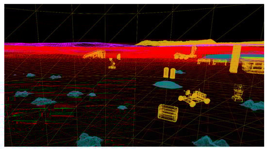
Figure 2.
Wireframe view of scene objects.
2.3. Complex Lunar Illumination Modeling
The lunar surface, covered by low albedo and retroreflective regolith, significantly affects its reflectivity. The illumination conditions are influenced by the absence of atmospheric and the unique properties of the regolith, resulting in strong lighting with extremely long shadows and high dynamic illumination range. To accurately simulate these conditions, we used ray tracing to create reflection lighting effects within craters, rock shadows, and objects like rovers. We optimized the lighting model to better represent the lunar surface’s dynamic range of illumination. The original model relied solely on direct sunlight, resulting in completely black-shadowed areas, unlike real lunar images where light reaches shadowed regions through surface scattering, earthshine, and starlight. Consequently, we introduced an enhanced ray tracing model that provides low-intensity light source compensation for shadowed areas and adjusted the intensity and angle of sunlight. We modeled the color temperature, irradiance, and angular diameter of the sun to more accurately simulate the lighting conditions of the lunar polar regions. The comparison between the original illumination model and the improved illumination model is shown in Figure 3.
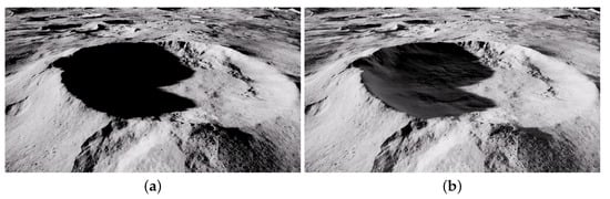
Figure 3.
Lighting model comparison: (a) Original lighting model effect. (b) Our improved lighting model effect.
2.4. Lunar Surface Stereo Vision System Modeling
Unreal Engine 4 (UE4) supports detailed modeling of camera parameters, including focal length, sensor size, and aperture, as well as various types of lens models, such as perspective and orthographic lenses. In our study, we employed two virtual cameras to construct a stereo vision system for image data acquisition. This system utilizes the Z-buffer to render depth images and generates accurate depth maps based on the coordinates of each pixel, serving as the ground truth for depth.
In the created stereo vision system, the camera model follows the pinhole camera model with a focal length of 70 mm, a baseline distance of 300 mm, and a resolution of 1920 × 1080. The cameras are positioned approximately 8 m above the lunar surface, capturing images from a tilted downward view. This setup simulates the scenario of a stereo vision system deployed at a lunar base in the polar regions of the Moon for scene exploration and environmental monitoring. Ultimately, we generated multiple sets of lunar surface images and their corresponding depth and disparity ground truth maps under varying distances and conditions, as illustrated in Figure 4. These images will be used for the design and validation of the proposed algorithms.
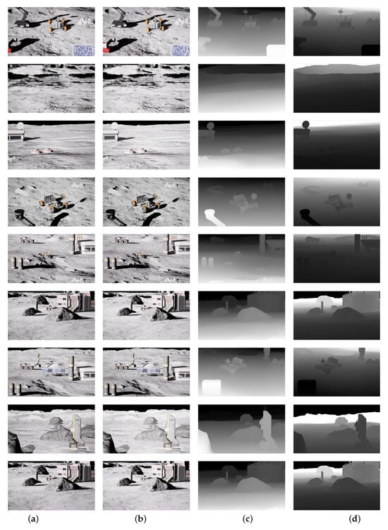
Figure 4.
Example of a lunar scene dataset created: (a) Left-camera image of the lunar scene. (b) Right-camera image of the lunar scene. (c) Disparity truth map of the left camera image. (d) Depth truth map of the left camera image.
To evaluate the performance of traditional methods in lunar surface scenarios, we conducted stereo matching using stereo images captured from a high-fidelity simulation of complex lunar terrain. The results, as shown in Figure 5, indicate that traditional algorithms perform suboptimally when applied to these challenging lunar images, particularly in areas with high-contrast lighting differences and weak textures, where noticeable errors occur. Consequently, it becomes evident that developing a stereo matching algorithm better suited to these environmental characteristics is critically important.
Figure 5.
Examples of the results from traditional stereo matching algorithms BM and SAD in lunar scenes: (a) Image data collected in our high-fidelity lunar scene physics simulation. This is the left image of a pair of stereo images. (b) Disparity map obtained using the BM algorithm, showing noticeable matching errors and disparity gaps, particularly in regions with weak textures and shadow occlusions. (c) Disparity map generated by the SAD algorithm, also exhibiting significant errors and disparity voids in texture-sparse and shadow-affected areas.
3. Proposed Methodology
Our work addresses the limitations of traditional stereo matching in lunar scenes, specifically tackling issues such as high-contrast lighting differences due to the Moon’s unique environment without an atmosphere and low surface reflectivity, the scarcity of lunar surface texture information, and extensive shadow occlusion areas caused by low solar angles. Our method includes two new technologies: First, we proposed an optimized Census transform multi-feature fusion cost calculation. We improved the original Census transform to enhance the sharing of neighborhood information in the cost calculation. We introduced pixel color intensity information to further improve the accuracy of the cost calculation, which not only reduces the impact of lighting on the lunar scene image but also refines the matching cost of weak texture areas in the scene. Second, we introduce a multi-layer superpixel disparity optimization method that combines coarse disparity maps with image data. By applying both global and local optimizations, our method effectively addresses shadow occlusion, significantly improving the accuracy of disparity estimation and resulting in a more detailed disparity map of the lunar surface. The workflow of our method is shown in Figure 6.
Figure 6.
Workflow of the proposed method. On the far left is our input stereoscopic image pair of the moon scene: (a) The process of our proposed optimized Census transform multi-feature fusion cost calculation. (b) The process of the multi-layer superpixel disparity optimization.
3.1. Optimized Census Transform Multi-Feature Fusion Cost Calculation
The Census transform is a non-parametric transform algorithm that encodes the differences between neighboring pixels and central pixels. It uses the Hamming distance to calculate matching costs. In this process, the grayscale values of the surrounding pixels within a window centered on pixel p are compared sequentially with the grayscale value of p. If a pixel’s value is greater than that of p, it is recorded as 0; otherwise, it is recorded as 1. The final matching cost is obtained by sorting these comparison values bitwise and applying Equation (2) to compute the Hamming distance.
In Equation (1), is the comparison function, p is the center pixel of the window, and q represents other pixels within the window centered on p. and are the intensity values of the respective pixels.
Since the calculation of matching costs is based on relative information between pixels rather than absolute values, it exhibits robustness to changes in illumination. However, this method has notable drawbacks. Firstly, it heavily relies on the center pixel p within the matching window, making it very sensitive to noise. Secondly, lunar scene images often contain many weakly textured areas, and this calculation method can result in matching errors in these regions. To address these issues, we propose the following improvements:
where represents the intensity difference threshold and is the weighted neighborhood intensity. The calculation method involves removing the maximum and minimum intensity pixels within the window and averaging the remaining pixel intensities to obtain . In Equation (3), the weighted intensity of pixels within the matching window replaces the central pixel intensity, and an intensity difference threshold is set to reduce dependence on the central pixel and suppress noise effects. Equation (4) represents the calculation of the optimized Census cost, where ⊗ denotes the bitwise concatenation operator. The calculation method is shown in Equation (3). Equation (5) non-linearly maps the calculated matching cost result to the 0–1 range, introducing to control the impact of cost, enhancing the differentiation of matching costs in weakly textured areas. Where represents the cost value of pixel at parallax , represents the calculated Hamming distance. Figure 7 illustrates examples of the original Census transform and our optimized Census transform. From a created lunar scene image, a window was randomly selected. It can be seen that when the central pixel is replaced with a noise pixel 100, the original Census transform fails, whereas our optimized Census transform remains unchanged, demonstrating its robustness against noise.
Figure 7.
Comparison of optimized Census transform and original Census transform in weakly textured areas: (a) The effect of noise on the original Census transform. (b) The effect of noise on the optimized Census variation method.
Additionally, in order to improve the matching ambiguity caused by the single Census feature when describing the cost, we introduce the color and intensity information of the pixel. These features help reduce matching ambiguity, so the pixel color scale was incorporated into the calculation of the matching cost to improve accuracy. This matching cost is calculated using Equation (6):
However, since the two costs have different scales, an exponential form in the [0–1] range was used to control the results, ensuring both cost values remain within this range. This approach prevents significant fluctuations in any single metric from affecting the outcome. The final matching cost is obtained by fusing these two costs and controlling the result within the [0–2] range.
After the completion of the matching cost calculation, we perform cost aggregation to fully leverage the pixel information from the neighborhood. This step aims to reduce noise and errors in the matching cost, ultimately enhancing the accuracy of the final disparity estimation. We have adopted a method similar to that of [28], utilizing cross-based aggregation to accumulate costs along multiple constructed paths. This proven approach is instrumental in achieving precise results.
where represents the cost of aggregation along path r. The matching cost calculation equation on each path is as follows:
where represents the multi-cost fusion matching cost. and are penalty coefficients used to penalize disparity changes between neighboring pixels. penalizes small disparity differences (i.e., a disparity difference of one pixel), while penalizes larger disparity differences (i.e., differences greater than one pixel). Generally, is smaller than . After obtaining the aggregated cost, the winner-takes-all (WTA) strategy is employed to select the optimal disparity, resulting in a coarse disparity map.
3.2. Multi-Level Superpixel Disparity Optimization
To enhance the accuracy of the final disparity estimation, particularly in addressing matching errors caused by extensive shadow occlusion resulting from the extremely low solar angle in the lunar south pole region, which is prevalent in lunar imagery, we further optimize the coarse disparity map obtained from the previous steps. Consequently, we propose a superpixel-based disparity optimization method based on the SDR approach [29]. Our method integrates input images and initial disparity maps for comprehensive disparity optimization and detailed correction of specific regions.
Specifically, the input images are first segmented into superpixels using the graph cut algorithm [30]. These segmented image regions serve as fundamental processing units, enhancing the stability of the image structure and providing a robust foundation for subsequent optimizations. The coarse disparity map is then refined through a combination of global and detail optimization strategies:
- 1.
- Global Optimization Layer: The mean disparity of superpixels is inferred using a Markov Random Field (MRF) framework. An energy function is established where the data term describes the superpixel disparity distribution via histograms, and the smoothness term enforces disparity consistency between neighboring superpixels.
- 2.
- Detail Optimization Layer: The Random Sample Consensus (RANSAC) method is employed to fit a slanted disparity plane for the superpixels. A probability-based disparity plane adjustment method is used to further refine the disparity map within the 3D superpixel neighborhood system, effectively addressing shadow occlusion issues.
In the global optimization layer, based on the principles of the Markov Random Field (MRF), the segmented superpixels are converted into graph nodes. The disparity for each superpixel is determined by minimizing the following energy function:
where s represents a superpixel, is the average disparity of the superpixel, denotes the data term, is the smoothness term, and is the balancing parameter for the smoothness term. Let be the set of all superpixels and on the set of neighboring superpixel pairs. Considering the irregular shapes of superpixels, the disparity distribution within a superpixel s is modeled as a normal distribution:
where d represents the disparity, and and represent the mean and variance of the superpixel’s disparity, respectively.
Next, neighboring superpixels with the same disparity are merged into new superpixels to facilitate subsequent detailed optimization. By evaluating the disparity differences between various superpixels, the three-dimensional spatial relationships among them are calculated. This determines the 3D neighborhood system of superpixels with disparity discontinuities. The calculation equation is as follows:
where represents a pair of superpixels. If their mean disparities are similar, denoted as , they belong to the same 3D neighborhood. Conversely, if their mean disparities are not similar, denoted as , they do not belong to the same 3D neighborhood. L represents the width of the disparity segments in the disparity histogram.
In the detail optimization layer, firstly, based on the initial disparity map, the RANSAC algorithm is employed to establish a slanted plane for each superpixel. Because we assumed earlier that the disparity distribution within each superpixel follows a normal distribution, an effective distribution should thus exhibit a unimodal distribution with a continuous range of disparities. To enhance the robustness of the algorithm, the disparity density distribution is used instead of the disparity distribution. The disparity density of the superpixel’s disparity d is defined as follows:
where L is the width of the disparity segment of the disparity histogram, and is the conditional judgment function, which is defined as follows:
Since the initial plane is generated by independently fitting each superpixel, this can lead to reduced disparity quality in regions with weak textures and occlusions. Therefore, local prior information is utilized probabilistically within the 3D neighborhood system established in the global optimization layer to effectively handle occlusions. Consequently, for a pair of superpixels belonging to a 3D neighborhood, the posterior probability of the disparity plane can be expressed as follows:
where are the observed values of the superpixel. Then, the weighted least squares method is used to estimate the slant plane of each superpixel, and finally, the filtering method is used to further refine it to obtain the final optimized lunar scene disparity map.
4. Experimental Results
4.1. Dataset Description
To evaluate the effectiveness of the proposed method, we conducted comprehensive tests using image data obtained from the high-fidelity complex lunar scene physical simulation described in Section 2. So far, we collected 20 sets of high-resolution lunar stereo image pairs for experimental evaluation, with imaging distances ranging from 10 to 100 m in the central area and image resolutions of 1920 × 1080 pixels.
Subsequently, we selected 5 pairs of representative lunar stereo images and their corresponding ground truth disparity maps to present the results, which are labeled as Scene 1, Scene 2, Scene 3, Scene 4, and Scene 5. These images simulate the presence of structures and equipment that might exist during the construction of lunar research stations, collectively forming complex lunar scene features. They cover typical lunar environment features, including high-contrast illumination changes, weak texture features, and shadow occlusion areas due to special lighting conditions. The primary objective of these experiments is to evaluate the proposed algorithm’s ability to handle texture variations and disparity estimation across scenes with different levels of detail. This is critical for ensuring the algorithm’s effectiveness in real-world applications, such as lunar surface exploration and the construction of scientific research stations on the Moon.
In addition, to avoid the possibility that the artificial structures we added might introduce extra textures into the images, we created a high-fidelity simulated scene without any artificial structures, more closely resembling the natural lunar environment, and conducted tests accordingly. We selected three pairs of representative image pairs, labeled as Scene 6, Scene 7, and Scene 8.
4.2. Parameter Settings
During the matching cost calculation, the size of the matching window M × N was set to 7 × 7, with an intensity threshold of 50. For the energy function, was set to 0.3, and the disparity segment width L in the data term was set to 2. The parameters and k for the superpixel segmentation were defined as in method 1, where is the Gaussian filter parameter for smoothing the influence of the input, and k affects the size of the segmented superpixels. In the lunar environment dataset, was set to 0.1 and k to 150. Additionally, the subsequent disparity optimization step required no parameters, demonstrating the robustness of this optimization.
4.3. Evaluation Metrics
In our experiments, we employed two standard stereo matching evaluation metrics: and L_RMS, as defined by Equations (17) and (18). represents the percentage of pixels where the disparity estimation deviates from the ground truth by more than a specified threshold . We set to 2.0 and 4.0. L_RMS represents the root mean square error between the estimated disparity and the ground truth, providing a comprehensive measure of the overall accuracy of the disparity estimation.
4.4. Comparative Analysis
To thoroughly validate the effectiveness of the proposed method, we compared it with several other approaches, including SGM [25] and StereoBM [13,18] algorithms which are widely used in the field of planetary exploration, AD-Census [28], which [5] has been a prominent stereo matching algorithm, and the deep learning-based method MC-CNN [31].
The visual results of our simulated image of the lunar research stations are presented in Figure 8. Panels (b)–(f) show the disparity map obtained by our proposed method and other stereo matching methods, while panel (g) represents the ground truth disparity map. The figure shows that SGM and BM exhibit significant errors and disparity inaccuracies in occluded regions. Although AD-Census does not show prominent invalid pixels, it has substantial errors at object boundaries and exhibits poor smoothness. In contrast, our method demonstrates superior performance across all three representative scenarios, producing visually smoother, more accurate disparity maps that effectively represent lunar surface scenes.
Figure 8.
Disparity estimation results for test images of the lunar research stations scene dataset. (b–f) represent the disparity estimation images of different methods in scenes 1-5 respectively. (a) Original image. (b) Disparity image obtained by SGM. (c) Disparity image obtained by StereoBM. (d) Disparity image obtained by AD Census. (e) Disparity image obtained by MC-CNN. (f) Disparity image obtained by Our method. (g) Ground truth disparity maps.
In addition to the aforementioned qualitative visual assessments, Table 1, Table 2 and Table 3 presents a quantitative evaluation of the effectiveness of our proposed method. By comparing the estimated disparity maps with the ground truth disparity maps, we utilized and L_RMS to assess the quality specifically. The results in Table 1, Table 2 and Table 3 clearly indicate that our method outperforms the other methods across all evaluated metrics.

Table 1.
Evaluation results of various advanced methods on representative data of lunar research stations scene dataset, on ‘bad 2.0’.
Table 2.
Evaluation results of various advanced methods on representative data of lunar research stations scene dataset, on ‘bad 4.0’.
Table 3.
Evaluation results of various advanced methods on representative data of lunar research stations scene dataset, on ‘L_RMS’.
To further assess the performance of the proposed method, we conducted tests using a high-fidelity simulation scene that closely replicates the natural lunar environment without the inclusion of any artificial structures. The purpose of this test was to evaluate the algorithm in a more realistic setting, where the natural surface features of the Moon—such as sparse textures, high-contrast lighting, and shadowed regions—are predominant, without the influence of additional textures introduced by man-made elements.
The test results are displayed in Figure 9. As shown, the proposed method demonstrates strong performance in these natural lunar conditions, maintaining accurate disparity estimates even in areas with low texture and significant shadow occlusion.
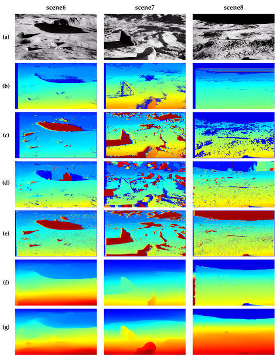
Figure 9.
Disparity estimation results for test images of the lunar research stations scene dataset. (b–f) represent the disparity estimation images of different methods in scenes 1–5 respectively. (a) Original image. (b) Disparity image obtained by SGM. (c) Disparity image obtained by StereoBM. (d) Disparity image obtained by AD Census. (e) Disparity image obtained by MC-CNN. (f) Disparity image obtained by Our method. (g) Ground truth disparity maps.
Table 4, Table 5 and Table 6 present the results of our quantitative analysis, which include the , , and L_RMS metrics. The quantitative analysis further corroborates the visual observations from Figure 9. Additionally, the L_RMS value of our method was significantly lower, indicating that our algorithm provides more consistent and accurate disparity estimation compared with the other methods. In conclusion, these tables provide a detailed comparison of our proposed method against traditional stereo matching algorithms, demonstrating its superior performance in handling weak textures, shadow occlusion, and large disparity discontinuities typically encountered in lunar surface environments.
Table 4.
Evaluation results of various advanced methods on representative data of lunar scene dataset, on ‘bad 2.0’.
Table 5.
Evaluation results of various advanced methods on representative data of lunar scene dataset, on ‘bad 4.0’.
Table 6.
Evaluation results of various advanced methods on representative data of lunar research stations scene dataset, on ‘L_RMS’.
4.5. Ablation Study
To evaluate the effectiveness of our proposed method, we conducted three sets of comparative experiments using images collected from simulated complex lunar scenes. Our process consists of the optimized Census transform multi-feature fusion cost calculation (Opt_Census) and superpixel disparity optimization (SDO), denoted as Opt_Census + SDO. We used the original Census method without any disparity optimization as the baseline for these experiments.
In the first set of comparative experiments, we compared the Opt_Census method with the original Census method while keeping all other components unchanged. The subsequent processing of the matching cost and the primary matching parameters, such as the size of the matching window (7 × 7) and the cost aggregation process, remained consistent with the Census method. This allowed us to specifically assess the improvements introduced by the Opt_Census method. In the second set of experiments, we introduced SDO into the Census method to evaluate the effectiveness of SDO. In the third set of comparative experiments, we combined SDO with the Opt_Census method based on the first set of experiments to evaluate the overall performance of the improved Census method with SDO. The visualization results of these three sets of experiments are shown in Figure 10.
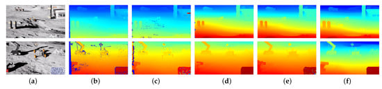
Figure 10.
Visual comparison of different methods on example images. The first and second rows are the results of two pairs of datasets in different combination experiments. They are denoted as Scene 1 and Scene 2, respectively: (a) Left image of the original image pair. (b–e) Disparity map of the Census, Opt_Census, Census + SDO, Opt_Census + SDO, respectively. (f) Ground truth disparity maps.
The results of the experiments are displayed in Table 7. It is clear that the Opt_Census method performs better than the original Census method, especially in accurately estimating discrepancies within shadow occlusion and weak texture regions. In the second and third sets of experiments, the inclusion of SDO significantly enhances both the Census and Opt_Census methods. Notably, Opt_Census + SDO produces the best results across all metrics, showcasing the superiority of our proposed method for estimating disparities in lunar surface scenarios.
Table 7.
Comparison results on the lunar scene dataset. The original Census, Opt_Census, Census + SDO, and Opt_Census + SDO are listed here. The evaluation indicators are “bad2.0”,”bad 4.0”, and “L_RMS”.
4.6. Test on Real Lunar Dataset
To further evaluate the performance of the proposed method, we conducted tests using real stereo images captured by the panoramic camera (PCAM) onboard China’s Yutu-2 lunar rover. This allows us to validate the algorithm’s robustness on actual lunar surface data. However, it is important to note that these images needed to undergo epipolar rectification before the stereo matching process, as accurate alignment is necessary to ensure high-quality disparity estimation. For the experiment, we randomly selected three representative lunar surface scenes from the Yutu-2 dataset. These scenes closely resemble the environments in our synthetic dataset and include typical lunar surface features such as low-texture regions, areas with high dynamic contrast, and shadowed occlusions. These characteristics are known to be particularly challenging for stereo matching algorithms, which makes this dataset a suitable candidate for assessing the robustness of our method.
Figure 11 presents the left-camera image from the selected Yutu-2 panoramic camera stereo image pair, along with the disparity maps estimated by our proposed method and other stereo matching methods for comparison. Each image pair has a resolution of 1176 × 864 pixels. We used the same parameter settings as described in the previous section to ensure consistency across experiments.
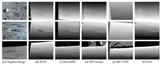
Figure 11.
Disparity estimation results for Yutu-2 real lunar scene dataset images: (a) The left-camera image from the stereo image pair captured by the Yutu-2 panoramic camera. (b–e) Disparity maps estimated by the stereo matching algorithm SGM, StereoBM, AD Census, and MCCNN. (f) Disparity map estimated by our proposed method.
The experimental results indicate the high dynamic contrast of the lunar surface, particularly in regions with both extreme brightness and deep shadows, was well managed, demonstrating the algorithm’s robustness in handling such harsh lighting conditions. The three selected stereo pairs encompass typical lunar surface characteristics, including rocks, occlusions, repeated patterns, and low-texture or even textureless areas. As evident from the experimental results, accurately estimating the disparity in shadow-occluded regions remains challenging. For instance, algorithms such as SGM and StereoBM struggle to provide accurate disparity estimates in these regions, while our method achieves better results. Additionally, in the third stereo pair, which includes large discontinuous disparity regions like the black sky background, methods such as AD Census and MC-CNN produce non-existent values. In contrast, our method effectively addresses these difficult areas, demonstrating superior performance in handling extreme disparity discontinuities. The disparity maps generated from the Yutu-2 images, though lacking ground truth for direct comparison, exhibit visually plausible depth estimates that align with known topographical features of the lunar surface.
5. Conclusions
In this paper, we propose a method using the Unreal Engine 4 (UE4) rendering engine for high-fidelity simulations to recreate complex lunar environments, addressing the scarcity of diverse lunar scene datasets. We focused on overcoming the challenges posed to traditional stereo matching by the high-contrast illumination variations resulting from the absence of atmosphere and low albedo of the lunar surface, as well as the sparse texture information due to the unstructured nature of the lunar terrain. To address these issues, we improved the Census transform cost computation method by optimizing the Census transform and incorporating a multi-cost fusion approach. This enhancement mitigated the impact of the Moon’s unique lighting conditions and improved disparity estimation in areas with weak textures. Additionally, we introduced a multi-layer superpixel disparity optimization method, which combines the initial disparity map obtained from the cost computation with superpixels segmented from the input images. This approach significantly improves the accuracy of disparity estimation in regions with extensive shadow occlusion, which are prevalent due to the low solar angles at the lunar poles.
In the experimental section, we conducted a comprehensive evaluation using image data generated from our high-fidelity physical simulation of complex lunar scenes. The results demonstrate that, compared with several representative classical stereo matching methods, our proposed approach effectively addresses the challenges posed by the unique lighting conditions, weak textures, and shadow occlusion present on the lunar surface. Consequently, our method not only enhances the accuracy of disparity estimation in lunar environments but also paves the way for new directions in stereo vision research for deep space exploration. We hope this work will inspire future research aimed at further optimizing stereo matching technology and expanding its applications in space exploration.
Author Contributions
Conceptualization, Z.L.; methodology, Z.L.; software, Z.L.; validation, Z.L., H.L., Z.Z. and Z.C.; investigation, Z.L. and H.L.; resources, R.Z. and E.L.; writing—original draft, Z.L.; writing-review and editing, H.L., Z.Z. and Z.C.; visualization, Z.L., Z.Z., J.Y. and Y.M.; supervision, E.L. and R.Z.; project administration, R.Z.; funding acquisition, R.Z. All authors have read and agreed to the published version of the manuscript.
Funding
This research was funded by Outstanding Youth Science and Technology Talents Program of Sichuan (2022JDJQ0027); the West Light of Chinese Academy of Sciences (No. YA21K001); Sichuan Province Science and Technology Support Program (No. 24NSFSC2625).
Data Availability Statement
The data presented in this paper will be released soon.
Acknowledgments
Thanks to the accompaniers working with us in department of the Institute of Optics and Electronics, Chinese Academy of Sciences.
Conflicts of Interest
The authors declare no conflicts of interest.
References
- Wei, R.; Yue, F.; Song, P.; Hong, Z.; Liyan, S.; Jinan, M. Landing Site Selection Method of Lunar South Pole Region. J. Deep Space Explor. 2022, 9, 571–578. [Google Scholar]
- Li, C.; Wang, C.; Wei, Y.; Lin, Y. China’s present and future lunar exploration program. Science 2019, 365, 238–239. [Google Scholar] [CrossRef] [PubMed]
- Israel, D.J.; Mauldin, K.D.; Roberts, C.J.; Mitchell, J.W.; P ulkkinen, A.A.; La Vida, D.C.; Johnson, M.A.; Christe, S.D.; Gramling, C.J. Lunanet: A flexible and extensible lunar exploration communications and navigation infrastructure. In Proceedings of the 2020 IEEE Aerospace Conference, Big Sky, MT, Canada, 7–14 March 2020; pp. 1–14. [Google Scholar]
- Andolfo, S.; Petricca, F.; Genova, A. Visual Odometry analysis of the NASA Mars 2020 Perseverance rover’s images. In Proceedings of the 2022 IEEE 9th International Workshop on Metrology for AeroSpace (MetroAeroSpace), Pisa, Italy, 27–29 June 2022; pp. 287–292. [Google Scholar]
- Zhang, H.; Sheng, L.; Ma, J. Comparison of the landing environments in lunar poles and some suggestions for probing. Spacecr. Environ. Eng. 2019, 36, 615–621. [Google Scholar]
- Zhang, H.; Du, Y.; Li, F.; Zhang, H.; Ma, J.; Sheng, L.; Wu, K. Proposals for lunar south polar region soft landing sites selection. J. Deep Space Explor. 2020, 7, 232–240. [Google Scholar]
- Menze, M.; Geiger, A. Object scene flow for autonomous vehicles. In Proceedings of the IEEE Conference on Computer Vision and Pattern Recognition, Boston, MA, USA, 7–12 June 2015; pp. 3061–3070. [Google Scholar]
- Scharstein, D.; Hirschmüller, H.; Kitajima, Y.; Krathwohl, G.; Nešić, N.; Wang, X.; Westling, P. High-resolution stereo datasets with subpixel-accurate ground truth. In Proceedings of the Pattern Recognition: 36th German Conference, GCPR 2014, Münster, Germany, 2–5 September 2014; pp. 31–42. [Google Scholar]
- Mayer, N.; Ilg, E.; Hausser, P.; Fischer, P.; Cremers, D.; Dosovitskiy, A.; Brox, T. A large dataset to train convolutional networks for disparity, optical flow, and scene flow estimation. In Proceedings of the IEEE Conference on Computer Vision and Pattern Recognition, Las Vegas, NV, USA, 27–30 June 2016; pp. 4040–4048. [Google Scholar]
- Guo, Y.Q.; Gu, M.; Xu, Z.D. Research on the Improvement of Semi-Global Matching Algorithm for Binocular Vision Based on Lunar Surface Environment. Sensors 2023, 23, 6901. [Google Scholar] [CrossRef] [PubMed]
- Wang, Y.; Gu, M.; Zhu, Y.; Chen, G.; Xu, Z.; Guo, Y. Improvement of AD-Census algorithm based on stereo vision. Sensors 2022, 22, 6933. [Google Scholar] [CrossRef] [PubMed]
- Pieczyński, D.; Ptak, B.; Kraft, M.; Drapikowski, P. LunarSim: Lunar Rover Simulator Focused on High Visual Fidelity and ROS 2 Integration for Advanced Computer Vision Algorithm Development. Appl. Sci. 2023, 13, 12401. [Google Scholar] [CrossRef]
- Scharstein, D.; Szeliski, R. A taxonomy and evaluation of dense two-frame stereo correspondence algorithms. Int. J. Comput. Vis. 2002, 47, 7–42. [Google Scholar] [CrossRef]
- Zhang, K.; Lu, J.; Lafruit, G. Cross-based local stereo matching using orthogonal integral images. IEEE Trans. Circuits Syst. Video Technol. 2009, 19, 1073–1079. [Google Scholar] [CrossRef]
- Pham, C.C.; Jeon, J.W. Domain transformation-based efficient cost aggregation for local stereo matching. IEEE Trans. Circuits Syst. Video Technol. 2012, 23, 1119–1130. [Google Scholar] [CrossRef]
- Stentoumis, C.; Grammatikopoulos, L.; Kalisperakis, I.; Karras, G. On accurate dense stereo-matching using a local adaptive multi-cost approach. ISPRS J. Photogramm. Remote Sens. 2014, 91, 29–49. [Google Scholar] [CrossRef]
- Maurette, M. Mars rover autonomous navigation. Auton. Robots 2003, 14, 199–208. [Google Scholar] [CrossRef]
- Matthies, L.; Huertas, A.; Cheng, Y.; Johnson, A. Stereo vision and shadow analysis for landing hazard detection. In Proceedings of the 2008 IEEE International Conference on Robotics and Automation, Pasadena, CA, USA, 19–23 May 2008; pp. 2735–2742. [Google Scholar]
- Woicke, S.; Mooij, E. Stereo vision algorithm for hazard detection during planetary landings. In Proceedings of the AIAA Guidance, Navigation, and Control Conference, National Harbour, MD, USA, 13–17 January 2014; p. 0272. [Google Scholar]
- Zabih, R.; Woodfill, J. Non-parametric local transforms for computing visual correspondence. In Proceedings of the Computer Vision—ECCV’94: Third European Conference on Computer Vision, Stockholm, Sweden, 2–6 May 1994; pp. 151–158. [Google Scholar]
- Li, T.; Liu, Y.; Wang, L. Evaluation for Stereo-vision Hazard Avoidance Technology of Tianwen-1 Lander. J. Astronaut. 2022, 43, 56–63. [Google Scholar]
- Boykov, Y.; Veksler, O.; Zabih, R. Fast approximate energy minimization via graph cuts. IEEE Trans. Pattern Anal. Mach. Intell. 2001, 23, 1222–1239. [Google Scholar] [CrossRef]
- Bobick, A.F.; Intille, S.S. Large Occlusion Stereo. Int. J. Comput. Vis. 1999, 33, 181–200. [Google Scholar] [CrossRef]
- Peng, M.; Liu, Y.; Liu, Z.; Di, K. Global image matching based on feature point constrained Markov Random Field model for planetary mapping. In Proceedings of the 32nd Asian Conference on Remote Sensing 2011, ACRS 2011, Tapei, Taiwan, 3–7 October 2011; pp. 373–378. [Google Scholar]
- Hirschmuller, H. Stereo processing by semiglobal matching and mutual information. IEEE Trans. Pattern Anal. Mach. Intell. 2007, 30, 328–341. [Google Scholar] [CrossRef] [PubMed]
- Barnes, R.; Gupta, S.; Traxler, C.; Ortner, T.; Bauer, A.; Hesina, G.; Paar, G.; Huber, B.; Juhart, K.; Fritz, L. Geological analysis of Martian rover-derived digital outcrop models using the 3-D visualization tool, Planetary Robotics 3-D Viewer—Pro3D. Earth Space Sci. 2018, 5, 285–307. [Google Scholar] [CrossRef]
- Li, H.; Chen, L.; Li, F. An efficient dense stereo matching method for planetary rover. IEEE Access 2019, 7, 48551–48564. [Google Scholar] [CrossRef]
- Mei, X.; Sun, X.; Zhou, M.; Jiao, S.; Wang, H. On building an accurate stereo matching system on graphics hardware. In Proceedings of the IEEE International Conference on Computer Vision Workshops, Barcelona, Spain, 6–13 November 2011; pp. 467–474. [Google Scholar]
- Yan, T.; Gan, Y.; Xia, Z.; Zhao, Q. Segment-based disparity refinement with occlusion handling for stereo matching. IEEE Trans. Image Process. 2019, 28, 3885–3897. [Google Scholar] [CrossRef] [PubMed]
- Felzenszwalb, P.F.; Huttenlocher, D.P. Efficient graph-based image segmentation. Int. J. Comput. Vis. 2004, 59, 167–181. [Google Scholar] [CrossRef]
- Bontar, J.; Lecun, Y. Computing the stereo matching cost with a convolutional neural network. In Proceedings of the IEEE Conference on Computer Vision and Pattern Recognition, Boston, MA, USA, 7–12 June 2015; pp. 1592–1599. [Google Scholar]
Disclaimer/Publisher’s Note: The statements, opinions and data contained in all publications are solely those of the individual author(s) and contributor(s) and not of MDPI and/or the editor(s). MDPI and/or the editor(s) disclaim responsibility for any injury to people or property resulting from any ideas, methods, instructions or products referred to in the content. |
© 2024 by the authors. Licensee MDPI, Basel, Switzerland. This article is an open access article distributed under the terms and conditions of the Creative Commons Attribution (CC BY) license (https://creativecommons.org/licenses/by/4.0/).