A Validation of OLCI Sentinel-3 Water Products in the Baltic Sea and an Evaluation of the Effect of System Vicarious Calibration (SVC) on the Level-2 Water Products

Abstract

The monitoring of coastal waters using satellite data, from sensors such as Sentinel-3 OLCI, has become a vital tool in the management of these water environments, especially when it comes to improving our understanding of the effects of climate change on these regions. In this study, the latest Level-2 water products derived from different OLCI Sentinel-3 processors were validated against a comprehensive in situ dataset from the NW Baltic Sea proper region through a matchup analysis. The products validated were those of the regionally adapted Case-2 Regional Coast Colour (C2RCC) OLCI processor (v1.0 and v2.1), as well as the latest standard Level-2 OLCI Case-2 (neural network) products from Sentinel-3’s processing baseline, listed as follows: Baseline Collection 003 (BC003), including “CHL_NN”, “TSM_NN”, and “ADG443_NN”. These products have not yet been validated to such an extent in the region. Furthermore, the effect of the current EUMETSAT system vicarious calibration (SVC) on the Level-2 water products was also validated. The results showed that the system vicarious calibration (SVC) reduces the reliability of the Level-2 OLCI products. For example, the application of these SVC gains to the OLCI data for the regionally adapted v2.1 C2RCC products resulted in RMSD increases of 36% for “conc_tsm”; 118% for “conc_chl”; 33% for “iop_agelb”; 50% for “iop_adg”; and 10% for “kd_z90max” using a ±3 h validation window. This is the first time the effects of these SVC gains on the Level-2 OLCI water products has been isolated and quantified in the study region. The findings indicate that the current EUMETSAT SVC gains should be applied and interpreted with caution in the region of study at present. A key outcome of the paper recommends the development of a regionally specific SVC against AERONET-OC data in order to improve the Level-2 water product retrieval in the region. The results of this study are important for end users and the water authorities making use of the satellite water products in the Baltic Sea region.

1. Introduction

In recent decades, remote sensing data have become one of the most important data sources to assess the effect and impacts of climate change [1,2,3,4]. The Global Climate Observing System (GCOS) provides comprehensive observations that are required by the scientific community for monitoring climate change. Furthermore, water-leaving radiance (Lw) derived from satellite data has been designated an Essential Climate Variable (ECV) by GCOS.

Perhaps the most significant development in the field of coastal water remote sensing was the launch of ENVISAT’s Medium-Resolution Imaging Spectrometer (MERIS), which operated between 2002 and 2012. MERIS had a spatial resolution of 300 m, which allowed for coastal waters to be studied at an unprecedented spatial resolution [5,6,7]. However, the launch of the European Space Agency’s (ESA) Sentinel-3A in February 2016 and Sentinel-3B in April 2018 marked a new era of research and development in ocean-colour measurement and monitoring using spaceborne platforms, due to their high spatial resolution and revisit times (1–2 days). Originally developed from MERIS, the two Sentinel-3 satellites house a newly developed ocean-colour sensor, the Ocean and Land Colour Instrument (OLCI-A and OLCI-B). The sensor has 21 spectral bands, ranging from 400 nm to 1020 nm, including dedicated ocean-colour bands; these new state-of-the-art optical sensors possess unprecedented spatial, temporal, spectral, and radiometric resolutions for ocean-colour satellite monitoring.

In order to make water-leaving radiance (Lw) from different ocean-colour missions comparable, it must first be calibrated against high-quality in situ data [8]. This process is termed system vicarious calibration (SVC), and it is undertaken by applying SVC gains to the Lw. As noted by Mazeran and Ruescas [9], SVC for ocean-colour applications was first introduced by Gordon et al. [10], who recognised the requirement for such optical sensors to be precisely calibrated to accurately measure the often-minute Lw signal. These gains are defined as the ratio between the expected (measured in situ) and actual top of the atmosphere (TOA) radiances, at each wavelength band, received at the satellite sensor [9]. A correction, which represents the difference between the radiances observed in situ and those observed from the satellite sensor, termed the SVC gains, is applied to the satellite radiances such that they precisely match the in situ optical measurements [9]. In theory, this correction should improve the satellite radiance product; however, SVC gains differ between water regions and processing schemes, and therefore, the SVC gains EUMETSAT currently provide for Sentinel-3 OLCI-A and OLCI-B [11] effectively represent an average of SVC gains from their respective in situ measurement sites. These average gains are recalculated on an ongoing basis as new matchups (correspondence between in situ and TOA reflectance) are obtained over the lifetime of the mission. The SVC of OLCI data is based on the gains from the Marine Optical BuoY (MOBY) off the coast of Hawaii, which has also been used for SVC of various ocean-colour satellites operated by NASA (such as SeaWiFS and MODIS; [12]). Usually, SVC gains are applied during pre-launch, as well as post-launch (on-orbit) radiometric calibration [13], with the aim of retrieving a satellite-derived Lw within a spectrally independent uncertainty of 5% [8]. While SVC has always been applied to MODIS data, it has been implemented on OLCI-A data since June 2017, which means data from both missions are now comparable [14]. While the SVC is widely considered a requirement for adequate merging of multi-mission ocean-colour data, it is not clear if the derived gains applied to OLCI Sentinel-3 data are applicable for all types of optically complex waters, for example in the Baltic Sea. The analysis by Kyryliuk and Kratzer [15] and Kratzer and Plowey [16] showed that the results of the locally adapted processor (which did not include SVC gains) returned better results than the processor which used SVC. This was to be expected for the total suspended matter (TSM) product, as a regional parameterisation of the specific scatter had been applied according to Kratzer and Moore [17]. However, it is unlikely that the positive effect on the other water products was due solely to the local adaptation of the salinity and temperature parameters in the processor. The effect of the SVC gains on OLCI-derived Level-2 water quality products for the Baltic Sea region has yet to be isolated and quantified. While Kratzer and Plowey [16] found that the current SVC applied to OLCI Sentinel-3 data is not beneficial for the retrieval of Baltic Sea water products, the effect of SVC was not quantified in their study.

Due to the extensive body of research and in situ ground truth data available for the region, the Baltic Sea serves as the ideal case study for evaluating the use of remote sensing for coastal water quality monitoring. Additionally, this region represents one of the most optically complex sea waters globally, with a predominant Coloured Dissolved Organic Matter (CDOM) influence on the spectral absorption and reflectance signature [6,17,18,19,20] which is accompanied with relatively low particle scatter. Kirk [21] noted the Baltic Sea’s relatively high CDOM concentration for a brackish waterbody and the decreasing CDOM concentrations from the Bothnian Gulf southwards in relation to the proportion of river water in the marine water.

Here, we undertake a validation of the latest satellite-based water products for Chlorophyll-a (Chl-a), TSM, CDOM, and Secchi depth. A matchup analysis was undertaken between the latest Sentinel-3 OLCI-A and OLCI-B water quality products and newly aggregated in situ water quality data for the Baltic Sea region. Several products and processing schemes were assessed, and a comparison was undertaken to evaluate which performed favourably in the region. By combining in situ datasets from previous Sentinel-3 OLCI validation studies, such as Kyryliuk and Kratzer [15] and Kratzer and Plowey [16], as well as newly available in situ data from the Swedish national pelagic monitoring program (funded by the Swedish Agency for Marine and Water Management, SwAM), one of the most comprehensive validation datasets for Sentinel-3 OLCI water products in the north-western (NW) Baltic proper region to date was created. This validation of the latest OLCI Level-2 water products provides the ocean-colour community with valuable information on these product’s performance in the Baltic Sea region. The objectives of the research were to (1) validate the latest OLCI Level-2 water products in the region; (2) to assess the current EUMETSAT OLCI SVC gains on the Level-2 water products for the region; and (3) to assess the effects of changes in the Case-2 Regional Coast Colour (C2RCC) processor between v1.0 and v2.1, especially the revised TSM equation in v2.1, on the Level-2 water products for the region.

2. Materials and Methods

After the application of data quality flags and the respective matchup time windows, matchup datasets ranging between n = 29 and n = 171 were obtained for the different OLCI-based water products. These satellite/in situ matchup data pairs were used to validate (1) the latest products of the neural network-based C2RCC processor; (2) the latest EUMETSAT SVC gains; and (3) the latest EUMETSAT Level-2 OLCI standard NN products.

The C2RCC OLCI outputs “conc_chl”, “conc_tsm”, “iop_agelb” and “iop_adg”, as well as “kd_z90max” (from both C2RCC v1.0 and v2.1) were validated against their respective in situ measurements. The “iop_agelb” and “iop_adg” products were both taken as proxies for CDOM [15], while “kd_z90max” was taken as a proxy for Secchi depth [15]. The C2RCC OLCI-based water quality products were processed in the following three ways: (1) Sentinel-3 OLCI C2RCC v1.0 without SVC; (2) Sentinel-3 OLCI C2RCC v2.1 without SVC; and (3) Sentinel-3 OLCI C2RCC v2.1 with SVC applied.

Additionally, some of the EUMETSAT Level-2 standard water products from the Baseline Collection 003 (BC003) were also validated for the region; “CHL_NN”, “TSM_NN”, and “ADG443_NN”.

2.1. Region of Interest (ROI)

The Region of Interest (ROI), which includes the coastal waters of Svealand, is illustrated in Figure 1. This ROI represents a coastal optical Case-2 water environment, with in situ validation sampling stations spanning approximately 300 km along the east coast of Sweden, in the NW Baltic proper region.

2.2. Matchup Data

Two types of data are required to perform a satellite-based matchup analysis; (1) extensive in situ validation data are required to ensure that enough in situ samples can be temporally and spatially matched to the satellite data; and (2) satellite data which are spatially and temporally coincident with at least some of the in situ data points. The following sections discuss the acquisition, matchup, and processing of both the in situ validation data and satellite data used in this study.

2.2.1. Validation Data

As part of this study, we aggregated in situ water quality datasets from three sources to create an extensive validation dataset of water quality products for the Baltic Sea proper region. These three in situ datasets, collected between May 2016 and August 2022, were comprised of ship-based discrete water samples for the four optically active constituents, which were: TSM (g m⁻³), Chl-a (µg L⁻¹), CDOM absorption (m⁻¹), and Secchi depth (m). The three datasets from which the new aggregated dataset was created were:

• Kyryliuk and Kratzer [15] dataset (referred to as: KYKR).
• Kratzer and Plowey [16] dataset (referred to as: PLKR).
• Swedish National Marine Monitoring Program (SwAM) dataset (referred to as: monitoring group (MG)).

Chl-a was measured spectrophotometrically using the trichromatic method [26,27]. The samples from MG were extracted in ethanol, while those from Kyryliuk and Kratzer [15] and Kratzer and Plowey [16], provided by the Marine Remote Sensing Group (MRSG) at Stockholm University, were extracted in acetone. The samples from the two laboratories have been shown to lie within a 5% difference in several intercomparisons of methods [28]. TSM was measured gravimetrically, following the method detailed in Strickland and Parsons [29] and the MERIS protocols [30], while turbidity was measured as outlined by Kari [31]. Finally, CDOM was measured spectrophotometrically using the method described by Kratzer and Vinterhav [6].

The validation samples for Chl-a concentration ranged from 1.02 to 28.58 µg L⁻¹; TSM concentration ranged from 0.28 to 6.57 g m⁻³; the absorption of CDOM at 440 nm (a_CDOM) ranged from 0.28 to 1.4 m⁻¹; and Secchi depth measurements ranged from 3 to 11 m. All Secchi depth measurements were captured with the use of a water telescope, which improved the validation results in tests. Additionally, all water samples were surface samples, captured within an approximately <1 m depth from the water’s surface and at stations which have a depth greater than that which would be subject to the bottom effect. In the absence of TSM data, and where turbidity data were available, turbidity (FNU) was converted to TSM (g m⁻³) according to the algorithm derived by Kari [31] for the region, shown in Equation (1); this increased the number of TSM validation samples available for use in this study.

$$In\left(TSM\right)=0.97\times In\left(t\right)-0.081$$

(1)

where TSM = TSM concentration (g m⁻³) and t = turbidity (FNU).

The three in situ datasets were combined and cleaned, with duplicate, incomplete, or missing samples removed. This cleaned dataset was then used to identify spatio-temporal coincident matchup Sentinel-3 OLCI-A and OLCI-B products for the matchup analysis/validation. In keeping with the validation time windows used in previous studies in the region [7,15], the matchup analysis was undertaken using samples collected within both a ±2 h and ±3 h time window of the Sentinel-3 overpasses. These matchup time windows consider the coastal dynamics and thus the rate of change in the optical in-water conditions over time in the region [15,32]. Due to the 300 m spatial resolution of OLCI-A and OLCI-B, there was a possibility of near-land pixels to be mixed pixels of both land and water signals. Therefore, samples within a <424 m distance from land were identified and removed from the validation dataset, as this distance represents the diagonal length of a Sentinel-3 OLCI pixel (300 m × 300 m square pixel), to ensure that the respective pixel does not overlap with land. Additionally, this 424 m threshold also sought to reduce adjacency effects from land.

From the initial 2940 in situ samples, the resultant aggregated and cleaned matchup datasets contained 407 and 558 in situ samples coincident with the Level-1 satellite data, as well as 256 and 357 samples coincident with the Level-2 standard products, for the ±2 h and ±3 h time windows, respectively. However, this number was reduced in the final validation due to the application of the OLCI data quality flags, as shown in the N values in Section 3 and

Table 1. Number (N) of matchup products and samples for each OLCI product before and after the application of OLCI data quality flags.

	OLCI Product	Time Window	No. OLCI Matchup Products	No. Matchup Samples
Before Data Quality Flags
	OLCI Level-1	±2 h	180	407
		±3 h	190	558
	OLCI Level-2	±2 h	102	256
		±3 h	109	357
After Data Quality Flags
	C2RCC v1.0 (OLCI Level-1)	±2 h	70	135
		±3 h	82	180
	C2RCC v2.1 (OLCI Level-1)	±2 h	70	127
		±3 h	86	170
	C2RCC v2.1 (OLCI Level-1) SVC	±2 h	72	131
		±3 h	86	172
	EUMETSAT Level-2 (OLCI Level-2)	±2 h	80	133
		±3 h	96	181

. This was largely due to the high percentage of cloud cover observed for the Baltic Sea region [15,17,33,34], which meant that only a fraction of the in situ validation data was suitable for the validation of satellite products.

2.2.2. Satellite Data

Due to the coastal nature of the ROI, a 1 × 1 pixel validation window was used. Normally, it is recommended that a 3 × 3 aggregated macropixel window is used for the validation of Sentinel-3 OLCI satellite products; however, this is not always possible for near-coast regions where a limited number of pixels are available, and therefore a 1 × 1 pixel window can be used for match-up analysis in such environments [15,16,35].

Level-1 S3 EFR OLCI Data

Sentinel-3 Level-1 EFR OLCI products, from Baseline Collection 002 (BC002), were identified using SentinelSat API (v1.2.1) [36] which queried the Copernicus Open Access Hub [37] API using the in situ sample dates, times, and coordinates for each sample in the in situ dataset to find matchup Sentinel-3 OLCI-A and OLCI-B products. However, the Copernicus Open Access Hub has since been closed, and all products are currently available from the Copernicus Data Space Ecosystem [38]. Cloud masks were not used, which ensured all possible matchup products were identified. After the initial matchup, the validation time window was then narrowed to ±2 h and ±3 h, respectively, data quality flags were applied (see Section 2.2.2 (OLCI data quality flags)), and the resultant OLCI products were utilized to validate the processing chains.

Table 1 summarizes the number of Level-1 OLCI products and corresponding validation samples for each of the processing chains and validation time windows evaluated, before and after the application of the OLCI data quality flags. By default, no SVC gains were applied to this Level-1 OLCI-A and OLCI-B data at source. Supplementary Tables S1–S6 (see Supplementary Materials) show the final Level-1 EFR OLCI matchup products used for each of the three individual C2RCC processing chains, identified in Table 1, for both the ±2 h and ±3 h validation windows. Figure 2 below shows an overview of the full C2RCC processing and validation workflow for both the SVC and non-SVC Level-1 OLCI products.

Level-2 S3 WFR OLCI Data

The Level-2 Sentinel-3 OLCI-A and OLCI-B WFR products, from Baseline Collection 003 (BC003), were downloaded directly from the EUMETSAT Data Store [39]. As the matchup OLCI products were already identified by the Python (v3.4.5) script for the Level-1 OLCI products; another matchup was not necessary. These Level-2 OLCI products include the three EUMETSAT standard water quality products, namely (1) “CHL_NN”, (2) “TSM_NN”, and (3) “ADG443_NN”, which were validated. Table 1 shows the number of OLCI Level-2 products and corresponding validation samples for the EUMETSAT standard product processing chain for both the ±2 h and ±3 h validation time windows, before and after the application of the OLCI data quality flags. By default, SVC gains are applied to these Level-2 water products at source. Supplementary Tables S7 and S8 (see Supplementary Materials) show the final EUMETSAT Level-2 OLCI products used for the validation. As these are already Level-2 products, the validation processing chain was straightforward, as illustrated in the validation workflow diagram Figure 3.

OLCI Data Quality Flags

Sentinel-3 OLCI data quality flags were used to exclude problematic OLCI pixels from the validation, including cloud, land, and sun glint pixels, for example. The data quality flags used were informed by those used in the works of Kyryliuk and Kratzer, Kratzer and Plowey, and Cazzaniga et al. [15,16,40]. These data quality flags were applied in the “Pix Ext and Data Quality Flags” step illustrated in the workflow diagrams in Figure 2 and Figure 3.

Two types of data quality flags are used in this study, namely (1) the standard OLCI product data quality flags; and (2) the C2RCC data quality flags. For the Level-1 OLCI data, the data quality flags used by Kyryliuk and Kratzer [15], highlighted in grey in

Table 2. OLCI data quality flags evaluated from [15,16,40], alongside the final flags used for the C2RCC validation. Those highlighted in grey are the baseline quality flags used by [15].

OLCI Quality Flags Tested	Final Quality Flags
&& !quality_flags.land	c2rcc_flags.Valid_PE
&& !quality_flags.bright	&& !c2rcc_flags.Cloud_risk
&& !quality_flags.straylight_risk	&& !c2rcc_flags.Rhow_OOS
&& !quality_flags.invalid	&& !c2rcc_flags.Rtosa_OSS
&& !quality_flags.cosmetic	&& !quality_flags.sun_glint_risk
&& !quality_flags.sun_glint_risk
&& !quality_flags.dubious

, were used as the baseline data quality flags. Additional data quality flags identified by Kratzer and Plowey [16] and Cazzaniga et al. [40], also listed in Table 2, were evaluated individually using a Python script to find which data quality flags improved the validation results Pearson’s r value. It was found that of the flags evaluated, only the addition of one extra data quality flag (to the baseline quality flag expression), the “quality_flags.sun_glint_risk” flag, improved the validation results, with the remainder having almost no effect on the Pearson’s r value. Therefore, this data quality flag was added to the baseline quality flag expression, as illustrated in Table 2. The results of the data quality flag tests can be found in Supplementary Tables S11 and S12 (see Supplementary Materials). As noted, the application of data quality flags substantially reduced the number of suitable matchup products and in situ validation samples, as can be seen in Table 1. For the EUMETSAT Level-2 OLCI products, the EUMETSAT recommended data quality flags were applied [11], as shown in

Table 3. EUMETSAT Baseline Collection 003 Sentinel-3 OLCI Level-2 standard product’s recommended data quality flags [11].

EUMETSAT Standard Products Quality Flags
WQSF_lsb.WATER
AND NOT WQSF_lsb.INVALID
AND NOT WQSF_lsb.LAND
AND NOT WQSF_lsb.COSMETIC
AND NOT WQSF_lsb.SUSPECT
AND NOT WQSF_lsb.CLOUD
AND NOT WQSF_lsb.CLOUD_AMBIGUOUS
AND NOT WQSF_lsb.CLOUD_MARGIN
AND NOT WQSF_lsb.SNOW_ICE
AND NOT WQSF_lsb.HISOLZEN
AND NOT WQSF_lsb.SATURATED
AND NOT WQSF_lsb.HIGHGLINT
AND NOT WQSF_lsb.OCNN_FAIL

.

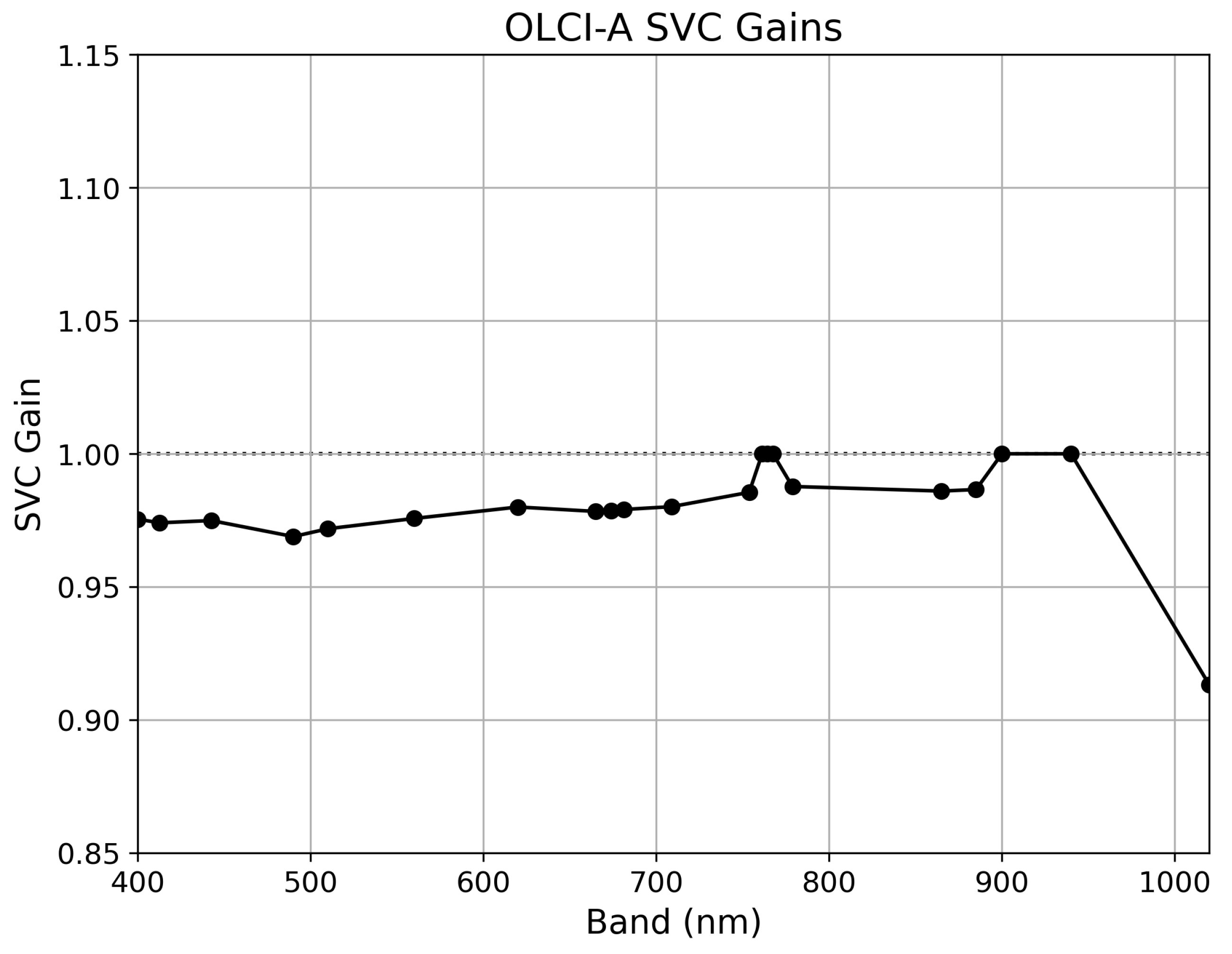
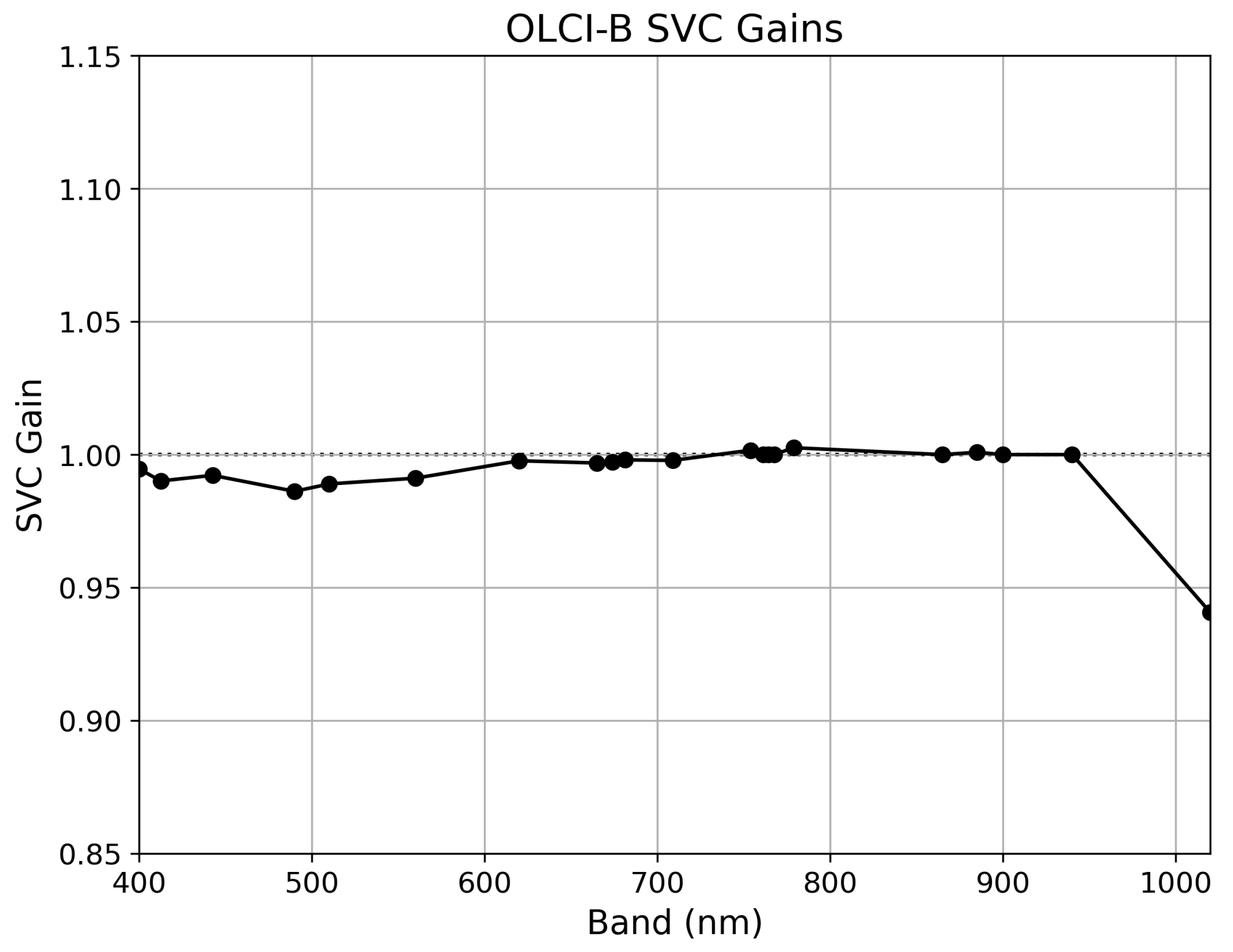
2.3. System Vicarious Calibration (SVC)

In this study, the effects of the current EUMETSAT SVC gains on these OLCI water products is validated for the region by applying these gains to the Level-1 OLCI radiance data prior to processing in C2RCC, and comparing the validation results to those where no SVC gains were applied. The latest EUMETSAT SVC gains [11] are graphed in Figure 4 and Figure 5, and can also be found in Supplementary Tables S9 and S10 (see Supplementary Materials). These SVC gains were applied to each Level-1 OLCI-A and OLCI-B radiance band by multiplying the band values of each pixel by the appropriate SVC gain value.

2.4. Case-2 Regional CoastColour (C2RCC)

The C2RCC processor is based on a machine learning (ML) neural network (NN) approach. The processor includes an atmospheric correction (AC) model which is coupled with a bio-optical model based on Hydrolight (Numerical Optics Ltd., Devon, UK), including several semi-analytical inherent optical properties (IOP) algorithms. Originating from Schiller and Doerffer [41] and Doerffer and Schiller [42], the Case-2 Regional processor (C2R) draws on a vast library of global IOP data to simulate an extensive range of optical water conditions sensed remotely over Case-2 waters (forward model). A vast library of IOPs with coinciding reflectance spectra is used to train the C2RCC NN. Subsequently, the water products (IOPs) are derived from the remote sensing reflectance via inverse modelling in an iterative way until the measured and simulated spectra match. The intermediate results are the scatter (b), as well as the absorption (a) at 442 nm. Using semi-analytical relationships, TSM is derived from b₄₄₂, while both the Chl-a concentration and the CDOM absorption are derived from a₄₄₂. The products can be regionally adapted by, for example, applying a mathematical relationship between the regionally specific IOP and the related water product, such as the TSM-specific scatter, and the TSM concentration. Initially, the C2R processor was trained on data from the North Sea [41] and has been tested successfully in the Baltic Sea [6,43].

Over time, the processor was further developed—using training data from other coastal waters—and renamed the Case-2 Regional CoastColour (C2RCC) [44]. The C2RCC processor is designed for use with Landsat-8 OLI, Sentinel-2 MSI, Sentinel-3 OLCI, MERIS, MODIS, VIIRS, and Sea WiFS. It is currently available as a Graphical User Interface (GUI) through SNAP, as a CLI, and through Python using the SNAP Python tool SNAPPY. In this work, the current version of C2RCC (v2.1), as well as the older C2RCC v1.0, was used through SNAP Version 9 and Version 6, respectively, through Python scripts using SNAPPY and the CLI to automate the processing. SNAP 10 has since been released, however the current version of C2RCC is still v2.1. The C2RCC OLCI processor outputs numerous Level-2 products, all of which are listed in

Table 4. C2RCC OLCI output products (adapted from [44]). Products in bold are those products validated in this study.

Output Level-2 C2RCC OLCI Products
Product	Description	Unit
	Reflectances
Rtoa 400–1020 nm	Top-of-atmosphere reflectance
Rrs 400–1020 nm	Atmospherically corrected angular dependent remote sensing reflectances	sr−1
Rhow 400–1020 nm	Normalized water-leaving reflectances
	Diffuse attenuation coefficient
kd489	Irradiance attenuation coefficient at 489 nm	m−1
kdmin	Mean irradiance attenuation coefficient at the three bands with minimum kd	m−1
kd_z90max	Depth of the water column from which 90% of the water-leaving irradiance comes from (1/kdmin)	m
	Inherent optical properties
iop_apig	Absorption coefficient of phytoplankton pigments at 443 nm	m−1
iop_adet	Absorption coefficient of detritus at 443 nm	m−1
iop_agelb	Absorption coefficient of Gelbstoff at 443 nm	m−1
iop_bpart	Scattering coefficient of marine particles at 443 nm	m−1
iop_bwit	Scattering coefficient of white particles at 443 nm	m−1
iop_adg	Detritus + Gelbstoff absorption at 443 nm (iop_adet + iop_agelb)	m−1
iop_atot	Phytoplankton + detritus + Gelbstoff absorption at 443 nm (iop_apig + iop_adet + iop_agelb)	m−1
iop_btot	Total particle scattering at 443 nm (iop_bpart + iop_bwit)	m−1
	Concentrations
conc_tsm	Total suspended matter dry weight concentration (v1.0: TSM = iop_bpart × 0.986 + iop_bwit × 1.72; v2.1: TSM = TSMfac × iop_btotTSMexp)	gm−3
conc_chl	Chlorophyll concentration (pow (iop_apig, 1.04) × 21.0)	mg m−3

along with a description of each.

2.4.1. C2RCC Parameterisation

This section describes the parameterisation of the regionally adapted C2RCC OLCI processor, largely based on the work of Kyryliuk and Kratzer [15]. However, some of these parameters were modified and updated for the latest version of the C2RCC processor (v2.1). Depending on the season, two different water temperature parameters were used [15]. For the months of April, May, and October 5 °C was used, and for June, July, August, and September 15 °C was used (C2RCC Default). Salinity was approximated at 6.5 PSU for the region; however, temperature and salinity values only have a minor influence on the results of the C2RCC processor [16]. The C2RCC v1.0 processing chain, termed “v1.0 Reg Adap”, used the same parameters as Kyryliuk and Kratzer [15], apart from the salinity, which was set to 6.5 instead of 7 used in the preceding study, as shown in

Table 5. C2RCC OLCI Processing Parameters. The “v1.0 Reg Adap” parameters are the same as those used by Kyryliuk and Kratzer [15], except for the salinity parameter, which was changed from a value of 7 PSU to a value of 6.5 PSU. “v1.0 Reg Adap”: C2RCC v1.0 with regionally adapted TSM parameters; “v2.1 Reg Adap”: C2RCC v2.1 with regionally adapted TSM parameters (same parameters used for “v2.1 Reg Adap SVC”); “v2.1 Def”: C2RCC v2.1 with default TSM parameters (same parameters used for “v2.1 Default SVC”). * 5 °C for April, May, October, 15 °C for June, July, August, September; ** New default value in C2RCC v2.1.

C2RCC OLCI Processing Parameters
	v1.0 Reg Adap	v2.1 Def	v2.1 Reg Adap
Valid-pixel expression	default	default	default
Salinity	6.5	6.5	6.5
Temperature	5, 15 *	5, 15 *	5, 15 *
Ozone	330	330	330
Air pressure	1000	1000	1000
TSM factor bpart (v1.0)	0.986
TSM factor bwit (v1.0)	1.72
TSM factor (v2.1)		1.06	1.212
TSM exponent (v2.1)		0.942	0.686
CHL exponent	1.04	1.04	1.04
CHL Factor	21	21	21
Threshold rtosa OOS	0.05	0.01 **	0.01 **
Threshold AC reflectances OOS	0.1	0.15 **	0.15 **
Threshold for cloud flag on transmittance down @865	0.955	0.955	0.955
Atmospheric aux data path	default	default	default
Alternative NN path	default	default	default
Output AC reflectances as Rrs instead of rhow	On	On	On
Derive water reflectance from path radiance and transmittance	Off	Off	Off
Use ECMWF aux data of source product	On	On	On
Output TOA reflectance	On	On	On
Output gas-corrected TOSA reflectance	Off	Off	Off
Output gas-corrected TOSA reflectances of auto NN	Off	Off	Off
Output path radiance reflectance	Off	Off	Off
Output downward transmittance	Off	Off	Off
Output upward transmittance	Off	Off	Off
Output atmospherically corrected angular dependent reflectances	On	On	On
Output normalized water-leaving reflectance	On	On	On
Output of out-of-scope values	Off	Off	Off
Output of irradiance attenuation coefficients	On	On	On
Output uncertainties	On	On	On

.

Due to the changes made between v1.0 and v2.1 of C2RCC, relating to how “conc_tsm” was calculated, a different TSM parameterisation was applied between the two versions. The equation used to relate the in situ concentration of TSM to both the marine and white particle scatter at 443 nm (“iop_bpart” and “iop_bwit”) was changed from a linear equation in v1.0 (Equation (2)) to an exponential equation in v2.1 (Equation (3)). It was also observed that the “iop_bpart” and “iop_bwit” outputs between v1.0 and v2.1 were notably different, meaning that the TSM equations were only compatible with their own version of the processor and not interchangeable between v1.0 and v2.1.

$$TSM=b_{part}·TSMfakBpart+b_{wit}·TSMfakBwit$$

(2)

where b_part is the C2RCC “iop_bpart” product and TSMfakBpart is its corresponding factor; b_wit is the C2RCC “iop_bwit” product and TSMfakBwit is its corresponding factor.

$$TSM=TSMfac·iop\_bto{t}^{TSMexp}$$

(3)

where TSMfac is the TSM factor, iop_btot is the C2RCC “iop_btot” product, and TSMexp is the TSM exponent.

Additionally, the default values changed for “Threshold rtosa OOS” and “Threshold AC reflectances OOS” between v1.0 and v2.1 of the processor, as shown in Table 5.

For C2RCC v1.0, the “TSM factor bpart” represents the inverse of the SPM-specific scatter in the Baltic Sea region [45], represented in Equation (4). Kratzer and Moore [17] calculated a mean SPM-specific scatter for the Baltic Sea ROI, which was 1.016 (±0.326 m² g⁻¹) (n = 56), resulting in a multiplicative inverse value of ~0.986 for “TSM factor bpart”; this is the value Kyryliuk and Kratzer [15] used, and as such, is the value used in C2RCC v1.0 in this study. As also informed by Kyryliuk and Kratzer [15], a “TSM factor bwit” value of 1.72 was used.

$$TSMfakBpart={\displaystyle \frac{1}{{b^{*}}_{p\left[SPM\right]}}}$$

(4)

where ${b^{*}}_{p\left[SPM\right]}$ = SPM-specific scatter.

For the first C2RCC v2.1 processing chain, termed “v2.1 Def”, the default TSM parameter values for the “TSM factor” and “TSM exponent” were used, as listed in Table 5. Following this, the regionally adapted “TSM factor” and “TSM exponent” values were used in the “v2.1 Reg Adap” processing chain, also shown in Table 5. These regionally adapted parameters were calculated using in situ particle backscatter (b_part) and corresponding TSM concentration (g m⁻³) data for the Baltic Sea region collected by Kratzer and Moore [17]. These b_part data were plotted against a_CDOM (m⁻¹) in Figure 6 (see Section 3). As shown in Equations (2) and (3), the variables “iop_bpart” and “iop_bwit” in the C2RCC v1.0 equation have been replaced in the v2.1 equation with a single variable representing the total scatter, “iop_btot”. This represents the total particle scatter of both marine particles and white particles (whitecaps) at 443 nm (iop_btot = iop_bpart + iop_bwit), as shown in Table 4. Using the in situ marine particle backscatter data (b_part), and assuming a white particle backscatter (b_wit) of 0 for the region, total particle backscatter (b_tot) was calculated as shown in Equation (5).

$$in\_situ\_b_{tot}=in\_situ\_b_{part}+in\_situ\_b_{wit}$$

(5)

where it was assumed that in_situ_b_wit = 0, as white caps are rarely observed in the Baltic Sea (unless during a storm).

The resultant in_situ_b_tot data were used with the corresponding in situ TSM concentration (g m⁻³) data to calculate the optimal values for both the “TSM factor” and “TSM exponent” parameters for “v2.1 Reg Adap”. The Generalized Reduced Gradient (GRG) solver method was used to vary the parameter values in Equation (3) to find the optimal values for the two parameters. This was carried out by minimizing the sum of the squared residuals (SSR) between the output “conc_tsm” and the in situ TSM concentration. The final TSM parameter values derived were a “TSM factor” of 1.212 and a “TSM exponent” of 0.686, with a final SSR value of 86. This showed an improvement over the default “TSM factor” and “TSM exponent” values, which returned an SSR of 238 when evaluated on the same data for the region. It was also observed that varying the C2RCC TSM parameter values does not affect the other outputs validated (“conc_chl”, “iop_agelb”, “iop_adg”, and “kd_z90max”). The final parameters used in each of the C2RCC v1.0 and v2.1 processing chains can be seen in Table 5.

2.4.2. Validation Difference Metrics

Equations (6)–(9) show the difference metrics used to assess the performance of each processor/processing chain [6,47]. These include Pearson’s correlation coefficient (r), Mean Normalised Bias % (MNB), Root Mean Square Difference % (RMSD), and Mean Absolute Percentage Difference % (MAPD).

$$\mathrm{Pearson}’\mathrm{s}r={\displaystyle \frac{{\sum }_{i=1}^N\left(OLC{I}_i-OLC{I}_i\right)\left(insit{u}_i-insit{u}_i\right)}{\sqrt{{\sum }_{i=1}^N{\left(OLC{I}_i-OLC{I}_i\right)}^2}\sqrt{{\sum }_{i=1}^N{\left(insit{u}_i-insit{u}_i\right)}^2}}}$$

(6)

$$\mathrm{Mean}\mathrm{Normalised}\mathrm{Bias}(\mathrm{MNB}\%)={\displaystyle \frac{1}{N}}\sum _{i=1}^N\left({\displaystyle \frac{OLC{I}_i-insit{u}_i}{insit{u}_i}}\right)\times 100$$

(7)

$$\mathrm{Root}\mathrm{mean}\mathrm{square}\mathrm{difference}(\mathrm{RMSD}\%)=\sqrt{{\displaystyle \frac{1}{N}}\sum _{i=1}^N{\left({\displaystyle \frac{OLC{I}_i-insit{u}_i}{insit{u}_i}}\right)}^2}\times 100$$

(8)

$$\mathrm{Mean}\mathrm{absolute}\mathrm{percentage}\mathrm{difference}(\mathrm{APD}\%)={\displaystyle \frac{1}{N}}\sum _{i=1}^N\left|ln\left({\displaystyle \frac{OLC{I}_i}{insit{u}_i}}\right)\right|\times 100$$

(9)

3. Results

Figure 6 shows the relationship between CDOM absorption (a_CDOM) and particle scatter (b_part) at 440 nm for the Baltic Sea, North Sea, English Channel, and the Adriatic Sea. As can be seen, this relationship is very different in the Baltic Sea compared to the other European Seas. For the same b_part at 440 nm values, the Baltic Sea’s a_CDOM (m⁻¹) values were found to be much higher than those of the North Sea, English Channel, and Adriatic Sea.

Table 6. Validation results for C2RCC (v1.0 and v2.1) “conc_tsm” for the Baltic Sea ROI, for both the ±2 h and ±3 h validation time windows. “Reg Adap”: regionally adapted TSM parameters. “Default”: default C2RCC TSM parameters. “Val Range”: validation data range. SVC results are highlighted in grey, while the best results are outlined in bold.

	v1.0 Reg Adap	v2.1 Default	v2.1 Default SVC	v2.1 Reg Adap	v2.1 Reg Adap SVC
TSM/conc_tsm (±2 h)
Pearson’s r	0.64	0.87	0.74	0.84	0.72
MNB	85%	144%	182%	135%	158%
RMSD	152%	202%	251%	179%	209%
MAPD/APD	105%	151%	186%	140%	161%
N=	47	39	41	39	41
Val Range (g m3)	0.28–6.17	0.28–6.17	0.28–6.17	0.28–6.17	0.28–6.17
TSM/conc_tsm (±3 h)
Pearson’s r	0.65	0.87	0.68	0.85	0.66
MNB	92%	146%	188%	133%	162%
RMSD	164%	202%	258%	176%	212%
MAPD/APD	111%	151%	192%	137%	165%
N=	66	59	59	59	59
Val Range (g m3)	0.28–6.17	0.28–6.57	0.28–6.17	0.28–6.57	0.28–6.17

shows the C2RCC “conc_tsm” validation results for each of the processing chains tested (both the ±2 h and ±3 h time windows); the SVC results are highlighted in the grey columns. The first column shows the regionally adapted v1.0 product’s validation results, which performed best for MNB, RMSD, and MAPD by a large margin. Although the v2.1 C2RCC products did perform best for Pearson’s r, this was accompanied by poor % MNB, RMSD, and MAPD values. Additionally, both SVC processing chains performed poorly when compared to the other processing chains validated. These key findings are discussed in greater detail in Section 4.

Table 7. C2RCC “v1.0” (no SVC), “v2.1” (no SVC), and “v2.1 SVC” (including SVC) validation results for: “conc_chl”, “iop_agelb”, “iop_adg” and “kd_z90max”. “Val Range”: validation data range. SVC results are highlighted in grey, while the best validation results are outlined in bold.

	v1.0 (±2 h)	v1.0 (±3 h)	v2.1 (±2 h)	v2.1 SVC (±2 h)	v2.1 (±3 h)	v2.1 SVC (±3 h)
Chl-a/conc_chl
Pearson’s r	0.49	0.47	0.68	0.4	0.64	0.4
MNB	−15%	−20%	17%	77%	15%	67%
RMSD	67%	66%	57%	194%	56%	174%
MAPD/APD	56%	56%	45%	95%	43%	84%
N	128	171	120	125	161	164
Val Range (μg L−1)	1.09–28.58	1.07–28.58	1.09–28.58	1.02–28.58	1.07–28.58	1.02–28.58
CDOM/iop_agelb
Pearson’s r	0.53	0.57	0.57	0.23	0.16	0.24
MNB	−69%	−70%	−80%	−57%	−74%	−65%
RMSD	72%	74%	81%	136%	85%	118%
MAPD/APD	69%	70%	80%	97%	83%	90%
N	36	55	29	30	48	48
Val Range (m−1)	0.33–1.4	0.28–1.4	0.33–1.4	0.33–1.4	0.28–1.4	0.28–1.4
CDOM/iop_adg
Pearson’s r	0.7	0.72	0.74	0.42	0.55	0.44
MNB	−26%	−32%	−39%	−1%	−35%	−13%
RMSD	60%	61%	51%	138%	62%	112%
MAPD/APD	55%	55%	47%	61%	51%	51%
N	36	55	29	30	48	48
Val Range (m−1)	0.33–1.4	0.28–1.4	0.33–1.4	0.33–1.4	0.28–1.4	0.28–1.4
Secchi depth/kd_z90max
Pearson’s r	0.12	0.14	0.59	0.15	0.5	0.13
MNB	26%	26%	−34%	−48%	−33%	−45%
RMSD	124%	120%	41%	54%	42%	52%
MAPD/APD	65%	63%	37%	50%	38%	48%
N	39	53	40	38	53	52
Val Range (m)	3.0–10.6	3.0–11.0	3.0–10.6	3.0–10.6	3.0–11.0	3.0–11.0

summarises the “conc_chl”, “iop_agelb”, “iop_adg” and “kd_z90max” C2RCC validation results for each of the processing chains, for both the ±2 h and ±3 h time windows. Like the “conc_tsm” results, the application of SVC did not improve the products’ overall validation performance, as shown in the grey columns. Both the “conc_chl” and “kd_z90max” products performed best in C2RCC v1.0, while the CDOM products (“iop_agelb”, “iop_adg”) performance was more closely matched between the two versions. As noted, the key findings are discussed in full in Section 4 below.

Table 8. EUMETSAT Sentinel-3 OLCI-A and OLCI-B Level-2 NN standard products validation results. Both ±2 h and ±3 h matchup time windows were validated. “Val Range”: validation data range. The best validation results are highlighted in bold.

TSM/TSM_NN
	TSM_NN (±2 h)	TSM_NN (±3 h)
Pearson’s r	0.77	0.66
MNB	209%	201%
RMSD	265%	263%
MAPD/APD	211%	204%
N	37	56
Val Range (g m3)	0.28–4.49	0.28–4.49
Chl-a/CHL_NN
	CHL_NN (±2 h)	CHL_NN (±3 h)
Pearson’s r	0.48	0.43
MNB	75%	63%
RMSD	135%	121%
MAPD/APD	89%	78%
N	127	173
Val Range (μg L−1)	1.09–28.58	1.07–28.58
CDOM/ADG443_NN
	ADG443_NN (±2 h)	ADG443_NN (±3 h)
Pearson’s r	0.36	0.39
MNB	−12%	−14%
RMSD	66%	69%
MAPD/APD	44%	46%
N	29	47
Val Range (m−1)	0.3–0.7	0.29–0.7

below summarises the validation results for the EUMETSAT Sentinel-3 OLCI Level-2 NN standard (non-regionally adapted) products; “TSM_NN”, “CHL_NN”, and “ADG443_NN”. These three standard products were outperformed by the regionally adapted C2RCC products, showing lower Pearson’s r values, and higher % MNB, RMSD, and MAPD values; this comparison will be discussed detail in Section 4 below.

4. Discussion

This section reviews the results presented in the previous section; beginning with the non-SVC C2RCC results, followed by the C2RCC SVC results, and finally the EUMETSAT Level-2 standard NN products’ results. The ±2 h and ±3 h validation results for each of the five C2RCC v1.0 and v2.1 (non-SVC and SVC) products have also been plotted in Supplementary Figures S1–S14 (see Supplementary Materials), allowing for a visual comparison between the results of each of the products validated. Additionally, the EUMETSAT Level-2 standard products’ validation results have been plotted in Supplementary Figures S15 and S16 (see Supplementary Materials).

4.1. C2RCC v1.0 vs. v2.1 Non-SVC

A comparison of the performance of C2RCC v1.0 and v2.1 (non-SVC) for each of the five water products (“conc_tsm”, “conc_chl”, “iop_agelb”, “iop_adg”, and “kd_z90max”) was undertaken using the newly aggregated in situ validation dataset, the results of which can be found in Table 6 and Table 7. It was found that the latest version of C2RCC (v2.1) outperformed the older version (v1.0) for both the Chl-a concentration (“conc_chl”) and Secchi depth product (“kd_z90max”), while the TSM product (“conc_tsm”) was retrieved more reliably using v1.0. The CDOM products (“iop_agelb” and “iop_adg”), showed less of a difference in performance between both versions of C2RCC than the other water products validated.

Despite the v2.1 “conc_tsm” returning higher Pearson’s r values for the validation, the % differences were much higher than those from v1.0 for MNB, RMSD, and MAPD. This overestimation of TSM was previously observed by Kyryliuk and Kratzer [15] in the region, and unfortunately, it has worsened in the latest version of the processor. Additionally, the processing chains with regionally adapted TSM parameters returned superior validation results than those which used the default TSM parameters. The CDOM products saw a significant decrease in Pearson’s r performance when the ±3 h matchup window was used instead of a ±2 h time window with C2RCC v2.1, with a substantial decrease in Pearson’s correlation coefficient, r, from 0.57 to 0.16 for “iop_agelb” and from 0.74 to 0.55 for “iop_adg”, a phenomenon not observed in the C2RCC v1.0 results. Furthermore, no significant gains in validation performance, for MNB, RMSD, and MAPD, were observed for the CDOM products when using the ±2 h instead of the ±3 h validation window, for both C2RCC v1.0 and v2.1, as was observed with the other three products validated. Higher % differences for MNB, RMSD, and MAPD were also observed for the “iop_agelb” CDOM product when using v2.1, while v1.0 and v2.1 “iop_adg” products performed more comparably. Overall, the older C2RCC v1.0 has proven to be more robust for the retrieval of TSM and CDOM products for the Baltic Sea ROI. Also of note, “iop_adg” outperformed “iop_agelb” when validated against the in situ CDOM data. The better performance of the “iop_adg” product is counter intuitive as this product is the sum of the absorption of organic particulate matter (detritus) + CDOM absorption, i.e., gelbstoff (iop_adet + iop_agelb) (see Table 4); however, similar results were already obtained before [15]. Also of note is the substantial improvement of the Secchi depth product (“kd_z90max”) in v2.1 over v1.0, with an increase in Pearson’s r from 0.12 to 0.59, a reduction in RMSD from 124% to 41%, and a reduction in MAPD from 65% to 37% observed in the validation of the newer version for the ±2 h validation window.

4.2. C2RCC v2.1 SVC

We found that the current EUMETSAT SVC gains [11] are not effective when applied to Sentinel-3 OLCI-A and OLCI-B data in the Baltic Sea region. This is likely due to relatively high CDOM absorption in these waters, as noted by Kratzer and Moore, Kowalczuk et al., and Kutser et al. [17,18,19]; and also observed here (Figure 6). For example, the CDOM product, “iop_adg”, returned a Pearson’s r value of 0.74 when SVC was not applied and 0.42 when SVC was applied. Additionally, an 87% difference in RMSD was observed between the two. Both CDOM C2RCC product’s (“iop_agelb” and “iop_adg”) MNB actually improved with the application of SVC gains, for example, by 23% and 38% respectively for the ±2 h validation window. However, this was accompanied by substantial increases in RMSD. Applying SVC gains worsened the MNB for TSM retrieval by 23%, Chlorophyll-a retrieval by 60%, and Secchi depth retrieval by 14% for the ±2 h C2RCC OLCI products. Due to the Baltic Sea being CDOM dominated, and the fact that SVC has been found to be detrimental to the retrieval of CDOM products, it is evident that the current EUMETSAT SVC gains are not suitable for application in the Baltic Sea region at this time. As mentioned in the introduction, the gains were derived from the MOBY station in Hawaii, which is situated in clear ocean waters, i.e., optical Case-1 waters [48] with high blue reflectance. The Baltic Sea, however, shows very low reflectance in the blue and highest reflectance in the green, around 560 nm [6,34,49].

It is worth noting that although the current EUMETSAT SVC gains had a negative effect on the C2RCC OLCI Level-2 water products, this effect may be different if other AC models and processors are used. Additionally, this poor performance is possibly due to the optical complexity of the Baltic Sea, which may make this ROI an outlier. Strictly speaking, these SVC gains were specifically derived for the standard processor over optical Case-1 waters using data from MOBY [9]. Nevertheless, they were later also applied to the C2RCC by EUMETSAT, even though the gains are not only sensor-specific, but may also vary with the processor applied (personal communication with Constant Mazeran, Solvo, France) [50]. Thus, the authors recommend that proceeding studies perform their own tests with and without SVC gains applied to the OLCI data, in order to determine the effect SVC has on their particular processing chains and ROI.

Kratzer and Plowey [16] previously identified that the SVC are a problem in the Baltic Sea, as the current SVC gains were not calculated using training data from the Baltic Sea region. The authors noted that more work needs to be done to improve SVC for the Baltic Sea waters. SVC gains for high CDOM waters could, for example, be derived from the AERONET-OC [51,52] site Gustaf Dahlen Light House in the north-western Baltic proper region, as well as the Palgrunden site in Lake Vänern [53]. Zibordi et al. [52] demonstrated the SVC of SeaWiFS and MODIS at two coastal AERONET-OC sites, the Acqua Alta Oceanographic Tower (AAOT) an oceanographic platform located 15 km from the Venice lagoon in the northern Adriatic as well as Gustaf Dalén Lighthouse Tower (GDLT), located 18km off the Swedish coast in the NW Baltic proper. They found that the gains from both sites were surprisingly quite similar, which was not expected for GDLT because of the optically complex waters of the Baltic Sea. The spectral signatures derived from GDLT also showed a relatively low variability due to the high CDOM influence, which may make this site (and other high CDOM sites) especially suited to derive system vicarious gains.

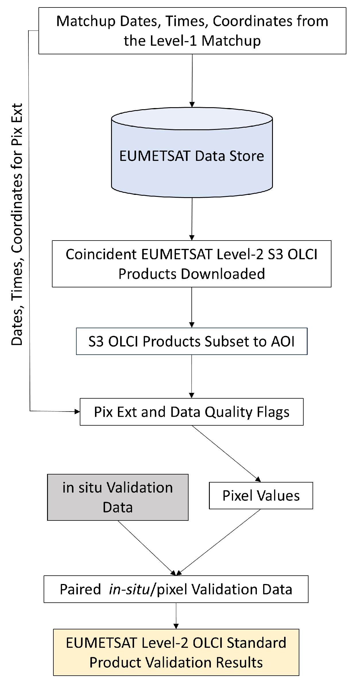
4.3. EUMETSAT Level-2 Products

The EUMETSAT Level-2 standard products “TSM_NN”, “CHL_NN”, and “ADG443_NN”, performed reasonably well in this validation, as shown in Table 8. However, these products were greatly outperformed by the regionally adapted C2RCC v2.1, with a Pearson’s r value of 0.66 vs. 0.85 for TSM, 0.43 vs. 0.64 for Chl-a, and 0.39 vs. 0.55 for CDOM (“ADG443_NN” vs. “iop_adg”) for the ±3 h validation time window. More importantly, these products exhibited much higher percentage differences than the regionally adapted C2RCC products, particularly for the TSM and Chl-a products. This is not surprising, considering these standard products are non-regionally adapted and developed for Europe-wide applications. As mentioned, C2RCC derives the IOPs from particle scatter and absorption at 440 nm which, in turn, are derived from the remote sensing reflectance and optimized in an iterative way. The relationship between CDOM absorption and particle scatter for the Baltic Sea, however, differs substantially when compared to other European Seas (Figure 6). Thus, it is unlikely that a general parametrization assumed for European waters would also hold for Baltic Sea waters. As these standard products are not regionally adapted, it was expected that they would underperform when compared to the regionally adapted C2RCC products [16].

Although no in situ radiometric data have been used in this study, the findings of previous studies, such as Cazzaniga et al. [40] and Kyryliuk and Kratzer [15], can be used to shed some light on the results of this study. Cazzaniga et al. [40], who utilized Aerosol Robotic Network (AERONET-OC) data [53] from Gustaf Dalen Lighthouse Tower, found that normalized water-leaving radiance (Lw) was largely overestimated in this ROI by both OLCI-A and OLCI-B. This overestimation was especially evident in the blue spectral region, where an overestimation of up to +81.7% for OLCI-A and +92.0% for OLCI-B for normalized Lw was observed. Cazzaniga et al. [40] attributed this overestimation in the blue spectral region to the high CDOM-dominated nature of the Baltic Sea’s waters, also illustrated in Figure 6. This phenomenon is likely a contributing factor to the accuracy of the OLCI-A and OLCI-B Level-2 water constituent products validated in this study; however, further research and in situ radiometric data would be required to confirm this. Similarly, Kyryliuk and Kratzer [15] observed an overestimation of remote sensing reflectance (Rrs) at the OLCI-A and OLCI-B 490nm band, which they attribute to a possible overcompensation of the Atmospheric Correction (AC) model for the blue bands in near-coast regions.

Additionally, the sample distance from land was plotted against APD from the C2RCC validation results, using the EEA coastline polygon [23]. This was undertaken to find if the adjacency effect was evident in the results. However, no correlation was found. This is probably because most in situ stations are found within rather close proximity to land, where the adjacency effects are highest. The validation sample distance from land ranged between ~424 m and 19.5 km (for one station), with the vast majority of samples being within <2 km of the coastline. Adjacency effects are known to decrease exponentially to a distance of about 36 km [54], and therefore have much less influence further offshore. Several corrections for the adjacency effect from land were developed for MERIS, such as the Improved Contrast between Ocean and Land processor, ICOL [55], and the SIMilarity Environment Correction, SIMEC [56]. ICOL showed a clear improvement in the remote sensing reflectance in the NW Baltic Sea for several MERIS processors [6], and SIMEC showed neutral, or positive effects when applied to MERIS data over lake Vänern [57]. Given that some of the adjacency corrections had already been developed for MERIS to provide improved reflectance retrieval in high CDOM waters, it is recommended that these corrections should also be made available for OLCI data.

5. Conclusions

This study evaluated the performance of the latest state-of-the-art Sentinel-3 OLCI-A- and OLCI-B-based Level-2 water constituent products for the Baltic Sea region. A comprehensive in situ validation dataset was used to evaluate each of the individual Level-2 water products and to compare their results. A number of conclusions can be drawn from the work, especially regarding the application of SVC gains, the comparison of C2RCC v1.0 and v2.1, and the performance of the EUMETSAT Level-2 OLCI standard products in the ROI. Here, recommendations on which processors/processing chains were found to perform best in the ROI will be made, based on the findings in this study.

Perhaps the most notable of these findings are those on the performance of the current Sentinel-3 OLCI SVC gains, provided by EUMETSAT [11]. This study found these SVC gains to be detrimental to the Level-2 water products when applied in the Baltic Sea region, and thus, a further development of suitable gains for this water region is highly recommended. The application of the current SVC gains resulted in poorer validation results for the ROI, which is in keeping with the current literature for the region [15,16].

We discovered that the regionally adapted C2RCC processor, without the application of SVC, performed best for constituent retrieval, across all constituents. Of the processing chains evaluated, C2RCC v2.1 without SVC performed best for Chl-a, and Secchi depth; while C2RCC v1.0 without SVC performed best for TSM and CDOM retrieval in the Baltic Sea ROI. C2RCC is known to overestimate TSM in the Baltic Sea, especially for extreme constituent concentrations [15]; as was observed in this study, with the current C2RCC v2.1 overestimating TSM even more so than v1.0 in the ROI. It is for this reason that the authors recommend the utilization of the older C2RCC v1.0 for TSM and CDOM retrieval in the region; or at the very least one should undertake a comparative validation study between the latest version and the older version for their respective ROI, as was undertaken here. Additionally, a natural degradation of Pearson’s r and % difference values of the validation results between the ±2 h and ±3 h validation time windows was also observed; this is of course expected and was most evident with the C2RCC v2.1 CDOM products, although it was quite minimal in most cases.

The current EUMETSAT Level-2 standard products performed respectably in the ROI when validated against the in situ validation data; however, these products were outperformed across all three products (“TSM_NN”, “CHL_NN”, and “ADG443_NN”) by the regionally adapted C2RCC products. These standard products were derived using the current EUMETSAT OLCI SVC gains, which have been proven to be ineffective for the Baltic Sea region; this is likely a contributing factor to the standard NN product’s inferior performance.

We recommend a more in-depth and robust validation of the current Sentinel-3 OLCI-A and OLCI-B reflectance products against spectral in situ radiometric measurements for the ROI. This would allow for the validation of various state-of-the-art AC procedures for water quality remote sensing in the region, and possibly the further development of these AC algorithms for the Baltic Sea. Additionally, other AC algorithms could be tested in the place of the C2RCC algorithm here, such as POLYMER [58]. However, Kratzer and Plowey [16] found POLYMER to perform less well than the regionally adapted C2RCC processor in the same ROI, likely because POLYMER was trained on North Sea data. Evidently, there is a need for Baltic-Sea-specific AC algorithms, given the findings of studies such as Cazzaniga et al. [40] and Kyryliuk and Kratzer [15] discussed in the previous section. The development of region-specific Sentinel-3 OLCI-A and OLCI-B SVC gains for the Baltic Sea would be extremely beneficial, as the current standard EUMETSAT SVC gains, from BC003, have proven inadequate when applied to C2RCC and the standard processor in the region; however, such undertakings are beyond the scope of this current study. This study represents the first time the effects of the current EUMETSAT OLCI SVC gains on the Level-2 water products have been isolated and quantified in the study region. This is an important contribution, as it informs the ocean-colour community of the performance of these current SVC gains in the region.

References

1. Aiken, J.; Moore, G.F.; Hotligan, P.M. Remote Sensing of Oceanic Biology in Relation to Global Climate Change. J. Phycol. 1992, 28, 579–590. [Google Scholar] [CrossRef]
2. Behrenfeld, M.J.; O’Malley, R.T.; Siegel, D.A.; McClain, C.R.; Sarmiento, J.L.; Feldman, G.C.; Milligan, A.J.; Falkowski, P.G.; Letelier, R.M.; Boss, E.S. Climate-driven trends in contemporary ocean productivity. Nature 2006, 444, 752–755. [Google Scholar] [CrossRef]
3. Yang, J.; Gong, P.; Fu, R.; Zhang, M.; Chen, J.; Liang, S.; Xu, B.; Shi, J.; Dickinson, R. The role of satellite remote sensing in climate change studies. Nat. Clim. Chang. 2013, 3, 875–883. [Google Scholar] [CrossRef]
4. Thomalla, S.J.; Nicholson, S.A.; Ryan-Keogh, T.J.; Smith, M.E. Widespread changes in Southern Ocean phytoplankton blooms linked to climate drivers. Nat. Clim. Chang. 2023, 13, 975–984. [Google Scholar] [CrossRef]
5. Doerffer, R.; Sorensen, K.; Aiken, J. MERIS potential for coastal zone applications. Int. J. Remote Sens. 1999, 20, 1809–1818. [Google Scholar] [CrossRef]
6. Kratzer, S.; Vinterhav, C. Improvement of MERIS level 2 products in Baltic Sea coastal areas by applying the Improved Contrast between Ocean and Land processor (ICOL)—Data analysis and validation. Oceanologia 2010, 52, 211–236. [Google Scholar] [CrossRef]
7. Beltrán-Abaunza, J.; Kratzer, S.; Höglander, H. Using MERIS data to assess the spatial and temporal variability of phytoplankton in coastal areas. Int. J. Remote Sens. 2017, 38, 2004–2028. [Google Scholar] [CrossRef]
8. Zibordi, G.; Mélin, F.; Voss, K.J.; Johnson, B.C.; Franz, B.A.; Kwiatkowska, E.; Huot, J.P.; Wang, M.; Antoine, D. System vicarious calibration for ocean color climate change applications: Requirements for in situ data. Remote Sens. Environ. 2015, 159, 361–369. [Google Scholar] [CrossRef]
9. Mazeran, C.; Ruescas, A. Ocean Colour System Vicarious Calibration Tool: Tool Documentation (DOC-TOOL). In Technical Report EUM/19/SVCT/D2; Issue: 1.0; EUMETSAT: Darmstadt, Germany, 2020; Available online: https://www.eumetsat.int/media/47502 (accessed on 26 September 2024).
10. Gordon, H.R. Calibration requirements and methodology for remote sensors viewing the ocean in the visible. Remote Sens. Environ. 1987, 22, 103–126. [Google Scholar] [CrossRef]
11. Sentinel-3 OLCI L2 report for baseline collection OL_L2M_003. In Technical Report EUM/RSP/REP/21/1211386; Issue: V2B; EUMETSAT: Darmstadt, Germany, 2021.
12. Clark, D.K.; Yarbrough, M.A.; Feinholz, M.; Flora, S.; Broenkow, W.; Kim, Y.S.; Johnson, B.C.; Brown, S.W.; Yuen, M.; Mueller, J.L. MOBY, a radiometric buoy for performance monitoring and vicarious calibration of satellite ocean color sensors: Measurement and data analysis protocols. In Ocean Optics Protocols for Satellite Ocean Color Sensor Validation—Volume 6: Special Topics in Ocean Optics Protocols and Appendices; National Aeronautics and Space Administration, Goddard Space Flight Center: Greenbelt, MD, USA, 2003. [Google Scholar]
13. Giannini, F.; Hunt, B.P.; Jacoby, D.; Costa, M. Performance of OLCI Sentinel-3A satellite in the Northeast Pacific coastal waters. Remote Sens. Environ. 2021, 256, 112317. [Google Scholar] [CrossRef]
14. Kwiatkowska, E.; Mazeran, C.; Brockmann, C.; Ruddick, K.; Voss, K.; Zagolski, F.; Antoine, D.; Bialek, A.; Brando, V.; Donlon, C.; et al. Requirements for Copernicus Ocean Colour Vicarious Calibration Infrastructure. In Technical Report SOLVO/EUM/16/VCA/D8; Issue: 1.3; EUMETSAT: Darmstadt, Germany, 2017; Available online: https://www.eumetsat.int/media/42725 (accessed on 26 September 2024).
15. Kyryliuk, D.; Kratzer, S. Evaluation of Sentinel-3A OLCI products derived using the Case-2 Regional CoastColour processor over the Baltic Sea. Sensors 2019, 19, 3609. [Google Scholar] [CrossRef] [PubMed]
16. Kratzer, S.; Plowey, M. Integrating mooring and ship-based data for improved validation of OLCI chlorophyll-a products in the Baltic Sea. Int. J. Appl. Earth Obs. Geoinf. 2021, 94, 102212. [Google Scholar] [CrossRef]
17. Kratzer, S.; Moore, G. Inherent Optical Properties of the Baltic Sea in Comparison to Other Seas and Oceans. Remote Sens. 2018, 10, 418. [Google Scholar] [CrossRef]
18. Kowalczuk, P.; Stedmon, C.A.; Markager, S. Modeling absorption by CDOM in the Baltic Sea from season, salinity and chlorophyll. Mar. Chem. 2006, 101, 1–11. [Google Scholar] [CrossRef]
19. Kutser, T.; Paavel, B.; Metsamaa, L.; Vahtmäe, E. Mapping coloured dissolved organic matter concentration in coastal waters. Int. J. Remote Sens. 2009, 30, 5843–5849. [Google Scholar] [CrossRef]
20. Soja-Woźniak, M.; Craig, S.E.; Kratzer, S.; Wojtasiewicz, B.; Darecki, M.; Jones, C.T. A novel statistical approach for ocean colour estimation of inherent optical properties and cyanobacteria abundance in optically complex waters. Remote Sens. 2017, 9, 343. [Google Scholar] [CrossRef]
21. Kirk, J.T.O. Light and Photosynthesis in Aquatic Ecosystems, 3rd ed.; Cambridge University Press: Cambridge, UK, 2010. [Google Scholar]
22. EMODnet Mean Depth Bathymetry. Available online: https://emodnet.ec.europa.eu/en/bathymetry (accessed on 2 August 2024).
23. EEA Europe Coastline Shapefile. Available online: https://www.eea.europa.eu/data-and-maps/data/eea-coastline-for-analysis-1/gis-data/europe-coastline-shapefile (accessed on 2 August 2024).
24. Natural Earth. Admin 0-Countries. Available online: https://aeronet.gsfc.nasa.gov/new_web/ocean_color.html (accessed on 2 August 2024).
25. Stockholm, Sweden Polygon. Available online: https://cartographyvectors.com/map/1331-stockholm-sweden (accessed on 2 August 2024).
26. Parsons, T.R.; Maita, Y.; Lalli, C. A Manual of Chemical and Biological Methods for Seawater Analysis; Elsevier: Amsterdam, The Netherlands, 1984; p. 173. [Google Scholar]
27. Jeffrey, S.W.; Mantoura, R.F.C.; Wright, S. Phytoplankton Pigments in Oceanography: Guidelines to Modem Methods, Appendix F; UNESCO Publishing: Paris, France, 1997; p. 661. [Google Scholar]
28. Kratzer, S.; Harvey, E.T.; Canuti, E. International Intercomparison of In Situ Chlorophyll-a Measurements for Data Quality Assurance of the Swedish Monitoring Program. Front. Remote Sens. 2022, 3, 866712. [Google Scholar] [CrossRef]
29. Strickland, J.; Parsons, T. A Practical Handbook of Seawater Analysis, 2nd ed.; Fisheries Research Board of Canada: Ottawa, ON, Canada, 1972; p. 310. [Google Scholar] [CrossRef]
30. Doerffer, R. Protocols for the Validation of MERIS Water Products; PO-TN-MEL-GS-0043; GKSS: Geesthacht, Germany, 2002. [Google Scholar]
31. Kari, E. Light Conditions in Seasonally Ice-Covered Waters. Ph.D. Thesis, Stockholm University, Stockholm, Sweden, 2017. [Google Scholar]
32. Beltrán-Abaunza, J.M.; Kratzer, S.; Brockmann, C. Evaluation of MERIS products from Baltic Sea coastal waters rich in CDOM. Ocean Sci. 2014, 10, 377–396. [Google Scholar] [CrossRef]
33. Karlsson, K. A 10 year cloud climatology over Scandinavia derived from NOAA Advanced very High Resolution Radiometer imagery. Int. J. Climatol. 2003, 23, 1023–1044. [Google Scholar] [CrossRef]
34. Reinart, A.; Kutser, T. Comparison of different satellite sensors in detecting cyanobacterial bloom events in the Baltic Sea. Remote Sens. Environ. 2006, 102, 74–85. [Google Scholar] [CrossRef]
35. Recommendations for Sentinel-3 OLCI Ocean Colour Product Validations in Comparison with In-Situ Measurements—Matchup Protocols; EUM/SEN3/DOC/19/1092968; Issue: V8B; EUMETSAT: Darmstadt, Germany, 2022.
36. SentinelSat API. Available online: https://sentinelsat.readthedocs.io/en/stable/ (accessed on 2 August 2024).
37. Copernicus Open Access Hub. Available online: https://scihub.copernicus.eu/ (accessed on 2 August 2024).
38. Copernicus Data Space Ecosystem. Available online: https://dataspace.copernicus.eu/ (accessed on 2 August 2024).
39. EUMETSAT Data Store. Available online: https://user.eumetsat.int/data-access/data-store (accessed on 2 August 2024).
40. Cazzaniga, I.; Zibordi, G.; Melin, F.; Kwiatkowska, E.; Talone, M.; Dessailly, D.; Gossn, J.I.; Muller, D. Evaluation of OLCI Neural Network Radiometric Water Products. IEEE Geosci. Remote Sens. Lett. 2022, 19, 1503405. [Google Scholar] [CrossRef]
41. Schiller, H.; Doerffer, R. Neural network for emulation of an inverse model operational derivation of Case II water properties from MERIS data. Int. J. Remote Sens. 1999, 20, 1735–1746. [Google Scholar] [CrossRef]
42. Doerffer, R.; Schiller, H. The MERIS Case 2 water algorithm. Int. J. Remote Sens. 2007, 28, 517–535. [Google Scholar] [CrossRef]
43. Attila, J.; Koponen, S.; Kallio, K.; Lindfors, A.; Kaitala, S.; Ylöstalo, P. MERIS Case II water processor comparison on coastal sites of the northern Baltic Sea. Remote Sens. Environ. 2013, 128, 138–149. [Google Scholar] [CrossRef]
44. Brockmann, C.; Doerffer, R.; Peters, M.; Kerstin, S.; Embacher, S.; Ruescas, A. Evolution of the C2RCC Neural Network for Sentinel 2 and 3 for the Retrieval of Ocean Colour Products in Normal and Extreme Optically Complex Waters. In Living Planet Symposium; Ouwehand, L., Ed.; ESA Special Publication: Paris, France, 2016; Volume 740, p. 54. [Google Scholar]
45. Kratzer, S.; Kyryliuk, D.; Brockmann, C. Inorganic suspended matter as an indicator of terrestrial influence in Baltic Sea coastal areas—Algorithm development and validation, and ecological relevance. Remote Sens. Environ. 2020, 237, 111609. [Google Scholar] [CrossRef]
46. Data Base of the EU MAST Project (MAS3-CT97-0087) COLORS: Coastal Region Long-Term Measurements for Colour Remote Sensing Development and Validation. Available online: http://databases.eucc-d.de/plugins/background/index.php (accessed on 2 August 2024).
47. Cristina, S.; Goela, P.; Icely, J.; Newton, A.; Fragoso, B. Assessment of water-leaving reflectances of oceanic and coastal waters using MERIS satellite products off the southwest coast of Portugal. J. Coast. Res. 2009, 1479–1483. [Google Scholar]
48. Morel, A.; Prieur, L. Analysis of variations in ocean color1. Limnol. Oceanogr. 1977, 22, 709–722. [Google Scholar] [CrossRef]
49. Ligi, M.; Kutser, T.; Kallio, K.; Attila, J.; Koponen, S.; Paavel, B.; Soomets, T.; Reinart, A. Testing the performance of empirical remote sensing algorithms in the Baltic Sea waters with modelled and in situ reflectance data. Oceanologia 2017, 59, 57–68. [Google Scholar] [CrossRef]
50. Mazeran, C.; SOLVO, Antibes, France. Personal communication, 2024.
51. D’Alimonte, D.; Zibordi, G.; Melin, F. A Statistical Method for Generating Cross-Mission Consistent Normalized Water-Leaving Radiances. IEEE Trans. Geosci. Remote Sens. 2008, 46, 4075–4093. [Google Scholar] [CrossRef]
52. Mélin, F.; Zibordi, G. Vicarious calibration of satellite ocean color sensors at two coastal sites. Appl. Opt. 2010, 49, 798. [Google Scholar] [CrossRef]
53. AErosol RObotic NETwork—Ocean Color (AERONET-OC) Program. Available online: https://www.naturalearthdata.com/downloads/10m-cultural-vectors/ (accessed on 2 August 2024).
54. Bulgarelli, B.; Zibordi, G. On the detectability of adjacency effects in ocean color remote sensing of mid-latitude coastal environments by SeaWiFS, MODIS-A, MERIS, OLCI, OLI and MSI. Remote Sens. Environ. 2018, 209, 423–438. [Google Scholar] [CrossRef] [PubMed]
55. Santer, R.; Zagolski, F. ICOL: Improve Contrast Between Ocean and Land; ATBD–MERIS level-1C; Rev. 1, Rep. D6 (1); University Littoral: Dunkerque, France, 2009. [Google Scholar]
56. Sterckx, S.; Knaeps, E.; Ruddick, K. Detection and correction of adjacency effects in hyperspectral airborne data of coastal and inland waters: The use of the near infrared similarity spectrum. Int. J. Remote Sens. 2011, 32, 6479–6505. [Google Scholar] [CrossRef]
57. Sterckx, S.; Knaeps, S.; Kratzer, S.; Ruddick, K. SIMilarity Environment Correction (SIMEC) applied to MERIS data over inland and coastal waters. Remote Sens. Environ. 2015, 157, 96–110. [Google Scholar] [CrossRef]
58. Steinmetz, F.; Ramon, D. Sentinel-2 MSI and Sentinel-3 OLCI consistent ocean colour products using POLYMER. In Remote Sensing of the Open and Coastal Ocean and Inland Waters; Frouin, R.J., Murakami, H., Eds.; SPIE: Bellingham, WA, USA, 2018; pp. 46–55. [Google Scholar] [CrossRef]
Figure 1. Map of the NW Baltic Sea ROI showing the matchup validation sample stations for the Sentinel-3 OLCI water products (within ±3 h) after the application of OLCI data quality flags. The red bounding box represents the ROI. All samples are >434 m from land, as noted in Section 2.2.1. Bathymetry data: [22]; Coastline Polyline: [23]; Countries Polygon: [24]; Stockholm Polygon: [25].
Remotesensing 16 03932 g001
Figure 2. C2RCC v2.1 validation workflow diagram for both the SVC and non-SVC regionally adapted C2RCC processing chains. The C2RCC v1.0 processing workflow was identical, apart from the processor version. The default, non-regionally adapted, C2RCC parameters were also validated. “KYKR” refers to the in situ dataset from Kyryliuk and Kratzer [15], “PLKR” refers to the Kratzer and Plowey [16] dataset, and “MG” is the Swedish National Marine Monitoring Program (SwAM) dataset. “Pix Ext” refers to “Pixel Extraction”.
Remotesensing 16 03932 g002
Figure 3. EUMETSAT Level-2 Sentinel-3 OLCI-A and OLCI-B Level-2 standard products validation workflow diagram. “Pix Ext” refers to “Pixel Extraction”.
Remotesensing 16 03932 g003
Figure 4. SVC gains for OLCI-A, Collection OL_L2M.003. Adapted from [11].
Remotesensing 16 03932 g004
Figure 5. SVC gains for OLCI-B in Collection OL_L2M.003. Adapted from [11].
Remotesensing 16 03932 g005
Figure 6. CDOM absorption (m−1) vs. bpart(440), showing the relatively high CDOM absorption observed in comparison to particle backscatter at 440 nm (bpart(440)) in the Baltic Sea region when compared to other European Seas. Baltic Sea data were obtained from Kratzer and Moore [17]. North Sea, English Channel, and Adriatic Sea data were obtained from the COLORS project [46].
Remotesensing 16 03932 g006