From Data to Decision: Interpretable Machine Learning for Predicting Flood Susceptibility in Gdańsk, Poland

Abstract

Flood susceptibility prediction is complex due to the multifaceted interactions among hydrological, meteorological, and urbanisation factors, further exacerbated by climate change. This study addresses these complexities by investigating flood susceptibility in rapidly urbanising regions prone to extreme weather events, focusing on Gdańsk, Poland. Three popular ML techniques, Support Vector Machine (SVM), Random Forest (RF), and Artificial Neural Networks (ANN), were evaluated for handling complex, nonlinear data using a dataset of 265 urban flood episodes. An ensemble filter feature selection (EFFS) approach was introduced to overcome the single-method feature selection limitations, optimising the selection of factors contributing to flood susceptibility. Additionally, the study incorporates explainable artificial intelligence (XAI), namely, the Shapley Additive exPlanations (SHAP) model, to enhance the transparency and interpretability of the modelling results. The models’ performance was evaluated using various statistical measures on a testing dataset. The ANN model demonstrated a superior performance, outperforming the RF and the SVM. SHAP analysis identified rainwater collectors, land surface temperature (LST), digital elevation model (DEM), soil, river buffers, and normalized difference vegetation index (NDVI) as contributors to flood susceptibility, making them more understandable and actionable for stakeholders. The findings highlight the need for tailored flood management strategies, offering a novel approach to urban flood forecasting that emphasises predictive power and model explainability.

1. Introduction

In the last 20 years, Europe has witnessed more than 400 major floods, affecting more than 8.7 million people, causing more than 2000 deaths, and resulting in losses of EUR 72 billion [1]. Projections for Central and Western Europe, including Poland, indicate a rise in pluvial and river floods [2]. Poland has faced severe urban floods in recent years, notably in Elblag (2017) [3], in Poznań and Swarzedz (2021) [2], and in Gdańsk (2001, 2016) [4,5]. These events often follow prolonged dry spells and are characterised by heavy and concentrated rainfall [6]. Identifying flood-prone areas and understanding the contributing factors are crucial to mitigating potential losses.

Flood susceptibility refers to the likelihood of an area experiencing flooding based on intrinsic characteristics, such as topographical, hydrological, and meteorological factors [7,8,9]. The goal of a flood susceptibility assessment is to develop models that determine the most relevant factors contributing to flood occurrence [10,11,12].

For flood susceptibility modelling, approaches vary from quantitative methods such as artificial intelligence, statistical techniques, and machine learning (ML) [11,13] to semi-quantitative methods like multi-criteria decision analysis (MCDA) [14]. Computational approaches include hydrologic–hydraulic [15] and hydrodynamic modelling [16] integrated with a geographical information system (GIS). Traditional hydrological and hydrodynamic models are time-consuming and prone to calibration issues, impacting their accuracy in identifying flood-prone regions [17]. MCDA models, although widely used, lack evaluation criteria [18].

In recent decades, ML techniques have gained momentum for effectively predicting flood-prone areas [18,19]. Among these, support vector machine (SVM), random forest (RF), and artificial neural network (ANN) have been widely applied to predict flood susceptibility. ANN is widely used for flood modelling because it can process non-linear and multivariate data, demonstrating universal modelling potential [10,20]. SVM and RF are also popular among hydrologists due to their prediction accuracy [10,11,13,21].

Despite the progress made in flood susceptibility modeling studies [10,11,13,17,20,21,22], significant challenges remain. A major issue is the lack of a universally accepted model for flood susceptibility due to their varying performances under different conditions and in different regions [22]. Furthermore, machine learning models are often criticised for being “black-box” models. The complexity and opacity of machine learning models often hinder their practical application, as stakeholders may need help understanding the factors driving the predictions. That is why there is high demand for models demonstrating how specific outcomes are achieved [17,23,24]. Many studies also fail to consider the interactions between different conditioning factors and classifiers, which are critical components for practical use.

This study addresses these gaps by introducing a novel combination of ensemble-based feature selection (EFFS) and explainable artificial intelligence (XAI) techniques for flood susceptibility modelling. Ensemble feature selection has demonstrated effectiveness across various domains, like human activity recognition [25], medical data analysis [26], and fish species data [27]. Despite its proven utility, its application in flood data analysis remains unexplored. This study aims to fill this gap by evaluating EFFS in the context of flood susceptibility modelling, focusing on Gdańsk, Poland.

The ensemble-based filter feature selection (EFFS) proposed in this study leverages the strengths of heterogeneous methods to create a more stable and optimal feature subset. Unlike other methods that rely solely on a single ranking mechanism or a small number of similar techniques, EFFS incorporates a diverse set of feature selection methods. This reduces the risk of bias or errors inherent in individual methods [25,27]. This approach enhances the performance of ML models by selecting the most relevant factors, resulting in improved flood susceptibility maps [28].

In addition to EFFS, this study incorporates a local XAI model, specifically the Shapley Additive exPlanations (SHAP) model [29,30] to provide transparency and acceptability regarding flood susceptibility in decision-making [24]. The use of SHAP allows for us to quantify the contribution of each feature to flood susceptibility predictions, making the results more interpretable and actionable for urban planners and stakeholders [17,31]. This is particularly important in the context of flood risk management, where understanding the influence of various environmental and infrastructural factors is crucial for decision making.

The main objectives of this study are as follows:

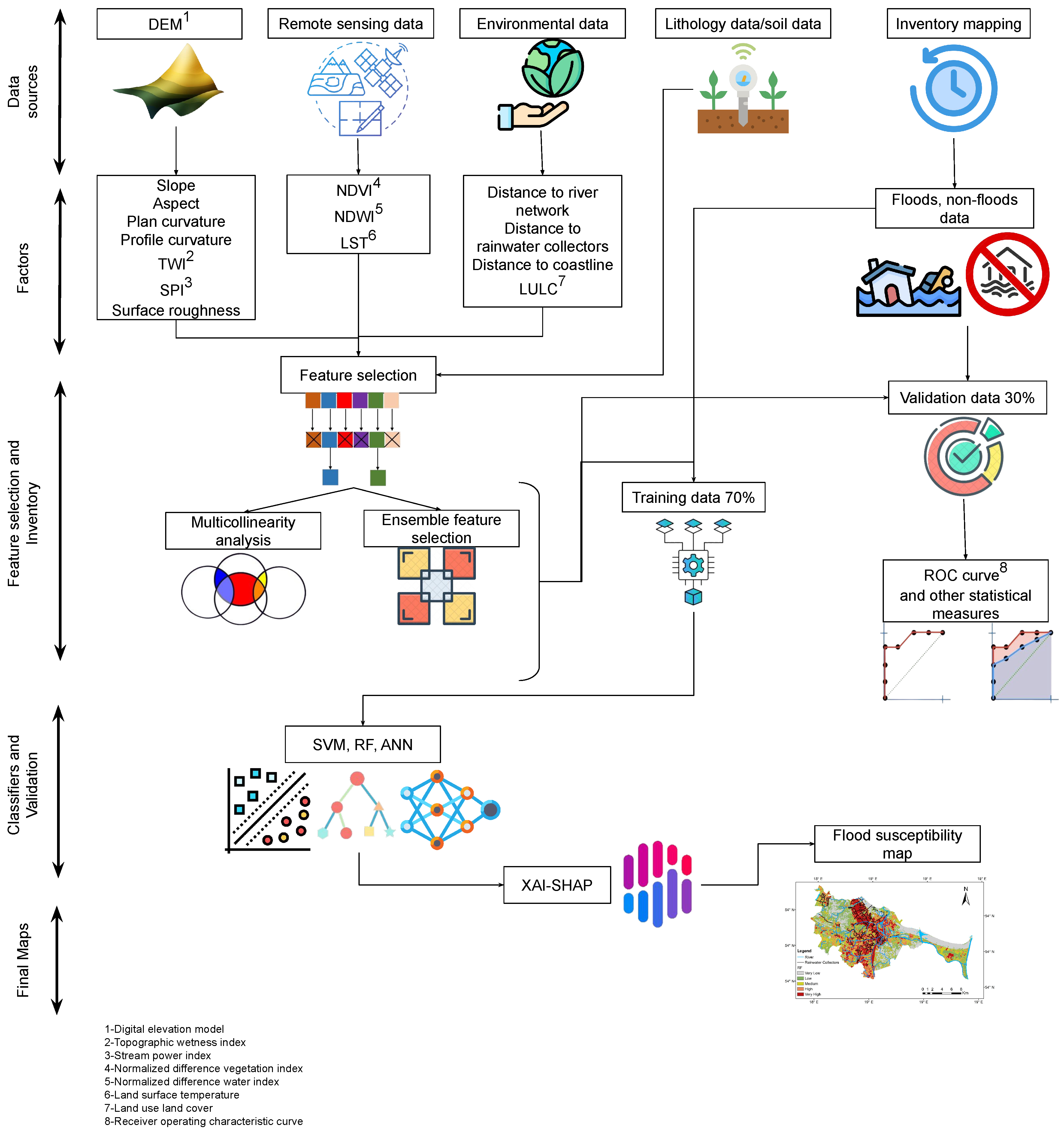
• To use machine learning models (SVM, RF, ANN) to effectively capture complex nonlinear interactions among hydrological, topographic, and built environment features.
• To introduce and assess the effectiveness of an EFFS method in optimising the selection of relevant flood conditioning factors.
• To incorporate explainable artificial intelligence to enhance the transparency and interpretability of the flood susceptibility models.

2. Datasets and Methodology

The methodology framework adopted in this study is shown in Figure 1 and encompasses several key steps: (i) flood inventory preparation; (ii) data collection on flood causative factors; (iii) data pre-processing in Python; (iv) multicollinearity analysis; (v) feature selection; (vi) model training and prediction; (vii) model validation and explanation; (viii) flood susceptibility map generation.

Figure 1. Workflow of flood susceptibility mapping using topographical and environmental data, feature selection, machine learning classifiers, and SHAP analysis.

2.1. Local Conditions and Fire Brigade Interventions Dataset

Gdańsk, the largest city in northern Poland, is located on the southern coast of the Baltic Sea in the Gulf of Gdańsk, covering an area of 262 km² (Figure 2). The coastal zone includes the Vistula Split, Vistula Delta Plain, and Kashubian Coast. Together with Sopot and Gdynia, Gdańsk forms the Tricity metropolitan area. The western side features the post-glacial hills of the Kashubian Lakeland, rising to 200 m above sea level. The southern part is a densely residential area, while the western part has elevated moraine hills and a plateau forming the Tri-City Landscape Park. In contrast, the eastern part has flat, low-lying polder areas called Żuławy Gdańskie, which are often below sea level [32,33].

Figure 2. The geographical location of the study area: map of Gdańsk, Poland (bottom left), Gdańsk in Pomeranian Voivodeship (bottom right), and a map of Gdańsk (top) showing flood event locations.

Gdańsk receives a mean annual precipitation of 659 mm [32]. Gdańsk faces three main flood hazards [34], as follows:

• Intensive precipitation and runoff from the Moraine Hills, causing urban flash floods, as seen in July 2001 and 2016 [35].
• High discharge or ice jams in the main Vistula channel.
• Sea level rises in the Bay of Gdańsk, and severe storm surges.

Although Gdańsk is not in an area with a high density of rainfall floods, its terrain makes it susceptible. Recorded rainfall episodes confirm this [35]. From 2010 to 2017, the State Fire Service Headquarters recorded 635 interventions related to sudden rainfall, peaking in 2016 (301), with the fewest occurringn in 2015 (10). On 15 July, 2016, the fire brigade intervened 189 times due to extreme rainfall on 14 July, 2016 (139.5 mm) [36].

Data for the analyses came from digital records of fire brigade interventions and flood event reports by Gdańskie Wody (Gdańsk Water Company; responsible for rainwater management in Gdańsk) [37]. Based on these data (Figure 2), a flood inventory map was prepared, depicting flooded and non-flooded locations, to train the ML models. The premise of the training was that future floods will follow past patterns. A total of 265 flood sites and an equal number of non-flood sites were selected, coded as 1 and 0. Following previous studies [11,22,38], the dataset was randomly split into training (70%) and test (30%) sets.

2.2. Collection of Factors Dataset

Flood intensity and severity depend on topographic, hydrologic, environmental, and geological factors [39,40]. This study selected flood susceptibility factors based on previous studies [13,21,26,38,41] and coastal city characteristics. The factors considered are presented in Table 1.

Table 1. Topographic, hydrologic, and environmental flood susceptibility factors selected for analysis.

Flood Susceptibility Factors	Equations	Sources
Elevation		1-m ALS DEM from Poland’s geoportal [42], ArcGIS 10.7
Slope		Derived from DEM
Aspect		Derived from DEM
Plan Curvature		Derived from DEM
Profile Curvature		Derived from DEM
Stream Power Index (SPI)	$\mathrm{SPI}=\alpha \times tan\beta$ 1	Derived from DEM [43]
Topographic Wetness Index (TWI)	$\mathrm{TWI}=log\left({\displaystyle \frac{\alpha }{tan\beta }}\right)$ 1	Derived from DEM [43]
Surface Roughness	$\mathrm{Roughness}={\displaystyle \frac{{\mathrm{FS}}_{\mathrm{mean}}-{\mathrm{FS}}_{\min }}{{\mathrm{FS}}_{\max }-{\mathrm{FS}}_{\min }}}$ 2	Derived from DEM, ArcGIS 10.7 [44]
Distance to Rainwater Collectors		Gdańskie Wody [45], scale 1:25,000
Distance to River Network		Open Street Map [46], updated using Gdańskie Wody
Distance from Coastline		System Informacji Przestrzennej Administracji Morskiej (SIPM) [47]
Soil		Polish Geological Institute—National Research Institute, spatial resolutions of 1:300,000 (2019–2021) and 1:50,000 [48]
Land Use		Urban Atlas 2018 from Copernicus land monitoring service (CLMS) [49]
Land Surface Temperature (LST)	$\mathrm{LST}={\displaystyle \frac{T_c}{1+(\lambda \times T_c/p)logϵ}}$ 3	Landsat 9 OLI/TIRS
NDVI (Normalized Difference Vegetation Index)	$\mathrm{NDVI}={\displaystyle \frac{\mathrm{NIR}-\mathrm{Red}}{\mathrm{NIR}+\mathrm{Red}}}$ 4	Landsat 9 OLI/TIRS
NDWI (Normalized Difference Water Index)	$\mathrm{NDWI}={\displaystyle \frac{\mathrm{NIR}-\mathrm{SWIR}}{\mathrm{NIR}+\mathrm{SWIR}}}$ 5	Landsat 9 OLI/TIRS

¹ $\alpha$ denotes cumulative upstream discharge or flow accumulation $\left({\mathrm{m}}^2{\mathrm{m}}^{-1}\right)$, and $\beta$ is the slope (in radians). ² $F{S}_{\mathrm{mean}}$, $F{S}_{\min }$, and $F{S}_{\max }$ represent the mean, minimum, and maximum focal statistical layer. ³ $T_c$ is the brightness temperature in Celsius; $\lambda$ is the emitted radiance wavelength; p is the result of ${\displaystyle \frac{h\times c}{b}}$ with h as the Planck’s constant, c as the velocity of light, and b as the Boltzmann constant; and $ϵ$ is the land surface emissivity (LSE). ⁴ NIR is infrared wavelengths, and R is red band. ⁵ NIR is infrared wavelengths, and SWIR is short-wave infrared band.

2.3. Data Preprocessing

All factors were standardised to 10 m resolution. The spatial database in raster format was created in ArcGIS-10.7, resulting in a matrix of 3380 columns by 1923 rows. Factor values across the study area and flood and non-flood sites were extracted in ArcGIS and exported as .csv files. Subsequently, the data were pre-processed using Python within the Google Collab. All factor values were normalised before model training using the MinMaxScaler from the sklearn module in Python. This technique scales the independent data to a range between 0 and 1, ensuring that all factors are on a consistent scale.

2.4. Multicollinearity Analysis of Flood Factors

Before training and validating the models, evaluating flood factors is crucial to identify noise and assess their predictive power to improve model accuracy [10,50].

Multicollinearity, assessed using variance inflation factors (VIF), is important in flood susceptibility studies. VIF quantifies how much the variance in a regression coefficient increases due to correlations among predictors [51]. A VIF value exceeding 5 suggests significant multicollinearity, which should be evaluated, and the removal of correlated factors from the model should be considered [52,53]. VIF is calculated using Equation (1):

$$VIF\left(x\right)={\displaystyle \frac{1}{1-R^2\left(x\right)}}$$

(1)

where $R^2\left(x\right)$ is the coefficient of determination when regressing an independent variable x against all other variables. A high $R^2\left(x\right)$ indicates a strong correlation between a flood and other factors.

2.5. The Ensemble-Based Filter Feature Selection (EFFS) Method

The EFFS technique, proposed to optimise feature sets [54], is applied in many research fields, such as control engineering [25] and cloud computing [28]. In this study, EFFS is adopted for the first time in flood susceptibility mapping, demonstrating its potential to enhance feature selection by leveraging the strengths of individual filter-based methods.

Initial feature importance rankings were obtained from the Mutual Information [11], Gain Ratio [25], Correlation [22], and ANOVA F-value [55] methods. These rankings form the basis for the subsequent ensemble analysis [25]. The outcome of the feature ranking using each method is expressed as follows:

$$\begin{array}{cc}\hfill AMI& =\left[XI\right(1),XI(2),...,XI(k),...,XI(m\left)\right];\hfill \end{array}$$

(2)

$$\begin{array}{cc}\hfill AGR& =\left[XG\right(1),XG(2),...,XG(k),...,XG(m\left)\right];\hfill \end{array}$$

(3)

$$\begin{array}{cc}\hfill ACO& =\left[XC\right(1),XC(2),...,XC(k),...,XC(m\left)\right];\hfill \end{array}$$

(4)

$$\begin{array}{cc}\hfill AAO& =\left[XO\right(1),XO(2),...,XO(k),...,XO(m\left)\right].\hfill \end{array}$$

(5)

Here, $XI\left(k\right),XG\left(k\right),XC\left(k\right)$, and $XO\left(k\right)$ represent the rank assigned to the kth feature by each respective filter-based method. The EFFS method integrates these individual rankings using a ’linear summation’ approach, where the ensemble score for each feature is calculated as the weighted sum of its ranks across the filter methods. The combined ranking is expressed as follows:

$$A=\left[X\right(1),X(2),...,X(k),...,X(m\left)\right],$$

(6)

where $X\left(k\right)$ denotes the ensemble score for the $kth$ feature, calculated as follows:

$$X\left(k\right)=\alpha XI\left(k\right)+\beta XG\left(k\right)+\gamma XC\left(k\right)+ϵXO\left(k\right)$$

(7)

The weights $\alpha$, $\beta$, $\gamma$, and $ϵ$ are empirically determined to balance the contributions from different filter methods. For this study, a weight combination of $(2,1,2,1)$ was chosen based on the preliminary results, although several other combinations were tested. Features were then sorted based on their ensemble scores in ascending order to finalise the ranking, ensuring optimal feature selection for flood susceptibility.

2.6. Models and Algorithms Used

Three ML models, i.e., (1) RF, (2) SVM, and (3) ANN, are used for predicting flood susceptibility. RF, an ensemble learning method, constructs numerous decision trees during training. Each tree is trained on a random data subset through “bagging”. The final RF output model, which handles classification and regression tasks, averages the predictions of individual trees:

$${\widehat{y}}_i={\displaystyle \frac{1}{M}}\sum _{j=1}^M{f}_j\left(x_i\right)$$

(8)

where M represents the total number of decision trees, $x_i$ refers to the input feature vector for the $x_i\mathrm{th}$ instance, ${\widehat{y}}_i$ is the final output from averaging the classification from individual decision tree prediction $f_j\left(x_i\right)$, $f_j$ is the classification model fitted on random dataset samples.

SVM, a supervised machine learning model, creates a hyperplane to maximise class separation using a kernel function. It employs a high-dimensional feature space and minimises structural risk through cross-validation, often using the Radial Basis Function (RBF) kernel for effective non-linear classification (Table 2). Support vectors, the training data points nearest to the hyperplane, help construct this hyperplane, which classifies new data based on the maximised margin between classes. The decision function (Equation (9)) is expressed as follows:

$$g\left(x\right)=\mathrm{sign}\left(\sum _{i=1}^n{y}_i{\alpha }_{j}K(x_i,x_j)+b\right)$$

(9)

where $g\left(x\right)$ represents the decision function for the SVM, $y_i$ is the label for the ith training instance, $K(x_i,x_j)$ denotes the kernel function, and b is the bias.

Table 2. Algorithm parameters selected for SVM, RF, ANN.

Algorithm	Parameters
SVM	Complexity parameter = 0.1; kernel = radial basis function; gamma = ‘auto’; probability = True
RF	n = 100, max_depth = 20; min_samples_split = 5
ANN	model = Keras sequential model; hidden layers = 4; nodes for each layer = 100, 40, 30, 1; activation = ‘relu’, ‘sigmoid’; optimiser = Adam; loss = ‘binary_crossentropy’; learning rate = 0.0013, epochs = 50
SHAP	Explainer = SVM: ‘KernelExplainer’; RF: ‘TreeExplainer’; ANN: ‘DeepExplainer’

Equation (10) represents the mathematical expression of RBF:

$$K(x_i,x_j)=exp(-\gamma \parallel x_i-x_j{\parallel }^2)$$

(10)

where $K(x_i,x_j)$ is the RBF kernel, $\gamma$ is the kernel coefficient that controls the influence of the distance between input vectors, and $\parallel x_i-x_j{\parallel }^2$ is the squared euclidean distance between input vectors $X_i$ and $X_j$.

Artificial Neural Networks (ANN) are computational models inspired by the human brain, comprising an input layer, one or more hidden layers, and an output layer. ANN uses a back-propagation algorithm for learning, adjusting its internal parameters (weights) based on the error between the predicted outputs and actual data. It minimises this error across training cycles [20,50]. The sigmoid function activates and handles non-linear relationships in the data. ANNs approximate complex functions in high-dimensional spaces, making them suitable for various applications, including classification and regression tasks in fields like hydrological modeling [41]. The net input to the neuron in the j layer is as follows:

$$ne{t}_j=\sum _i{w}_{ij}·o_i$$

(11)

where $w_{ij}$ is the weight connecting the node i to node j, and $o_i$ is the output from node i.

$$O_j=f\left(ne{t}_j\right)$$

(12)

where $O_j$ is the output from node j, and f is the activation function applied to the net input.

$$f^{\prime }\left(ne{t}_j\right)=f\left(ne{t}_j\right)·(1-f\left(ne{t}_j\right))$$

(13)

where $f^{\prime }\left(ne{t}_j\right)$ is the derivative of the activation function.

$$E={\displaystyle \frac{1}{2}}\sum _k{(d_k-o_k)}^2$$

(14)

where E is the total error, $d_k$ is the target output, and $o_k$ is the actual output from the output layer.

$$\Delta w_{ij}=-\eta {\displaystyle \frac{\partial E}{\partial w_{ij}}}$$

(15)

where $\Delta w_{ij}$ is the weight update, $\eta$ is the learning rate, and ${\displaystyle \frac{\partial E}{\partial w_{ij}}}$ is the partial derivative of the error with respect to the weight.

$$w_{ij}(n+1)=w_{ij}\left(n\right)+\Delta w_{ij}$$

(16)

where $w_{ij}(n+1)$ is the updated weight for the next iteration.

2.7. Model Explainability

Explainable artificial intelligence enhances transparency in machine learning models, enabling analysts to understand how factors influence model predictions. XAI techniques are categorised into global (permutation feature importance and mean decrease impurity) and local approaches (SHAP and Local Interpretable Model-Agnostic Explanations (LIME)). Global methods show overall significance for average predictions, while local methods make specific contributions to individual predictions [31,56]. This study employs the SHAP method [30] to determine how flood conditioning factors impact flood prediction outcomes.

SHAP values, calculated using the Python-based SHAP library, help to identify key drivers of the model’s outputs, enhancing interpretability in flood susceptibility modeling. The SHAP value ${\varphi }_i(f,x)$ quantifies the influence of factor i on the model prediction f for the input x, as shown in Equation (17). F represents all features while S is a subset of F excluding i [31]. The overall influence is measured by mean $\left|\mathrm{SHAP}\right|$ value value per feature.

$${\varphi }_i(f,x)=\sum _{S\subseteq F\backslash \left\{i\right\}}{\displaystyle \frac{\left|S\right|!\left(\right|F|-|S|-1)!}{\left|F\right|!}}\left(f_{S\cup \left\{i\right\}}\left(x_{S\cup \left\{i\right\}}\right)-f_S\left(x_S\right)\right)$$

(17)

$$I_j=-{\displaystyle \frac{1}{n}}\sum _{k=1}^n\left|{\varphi }_j^{\left(k\right)}\right|$$

(18)

where $I_j$ represents the average importance of feature j across all instances. n is the total number of instances in the dataset, and ${\varphi }_j^{\left(k\right)}$ denotes the SHAP value for feature j for the kth instance, which quantifies the contribution of feature j to the prediction for that particular instance.

Table 2 shows the explainers used for each model under SHAP.

Previously, research on ML models for flood susceptibility employed variable importance plots to highlight the most and least essential predictors [17,31]. However, these plots fail to elucidate crucial aspects, such as variable interactions leading to specific model outputs. Individual force plots and collective summary plots are utilised to address this limitation. These force plots provide a deeper understanding of how the variables interact and influence the outcomes.

2.8. Performance Evaluation

Flood susceptibility results are evaluated using several statistical metrics for training and test data: root mean squared error (RMSE), mean absolute error (MAE), accuracy (ACC), sensitivity, specificity, and area under the receiver operating characteristic ROC curve (AUC). The ROC is a standard criterion for evaluating model predictive power, plotting sensitivity on the y-axis and specificity on the x-axis. Sensitivity indicates the proportion of correctly classified flood cells, while specificity suggests the proportion of non-flood cells correctly classified as non-flood sites [10]. The area under the ROC curve, the AUC value, ranges between 0 and 1 and measures model performance, with values closer to 1 representing better performance and values closer to 0 indicating a non-informative model [19]. AUC, sensitivity, and specificity are given as follows:

$$\mathrm{AUC}={\displaystyle \frac{\sum TP+\sum TN}{P+N}}$$

(19)

$$\mathrm{Sensitivity}={\displaystyle \frac{TP}{TP+FN}}$$

(20)

$$\mathrm{Specificity}={\displaystyle \frac{TN}{FP+TN}}$$

(21)

P is the total number of flood pixels, and N is the total non-flood pixels. $TP$ (true positives) and $TN$ (true negatives) are correctly classified as flood and non-flood cells. $FP$ (false positives) and $FN$ (false negatives) are incorrectly classified as flood and non-flood cells. The ROC curve validated the final prediction maps for both training and test datasets.

3. Results

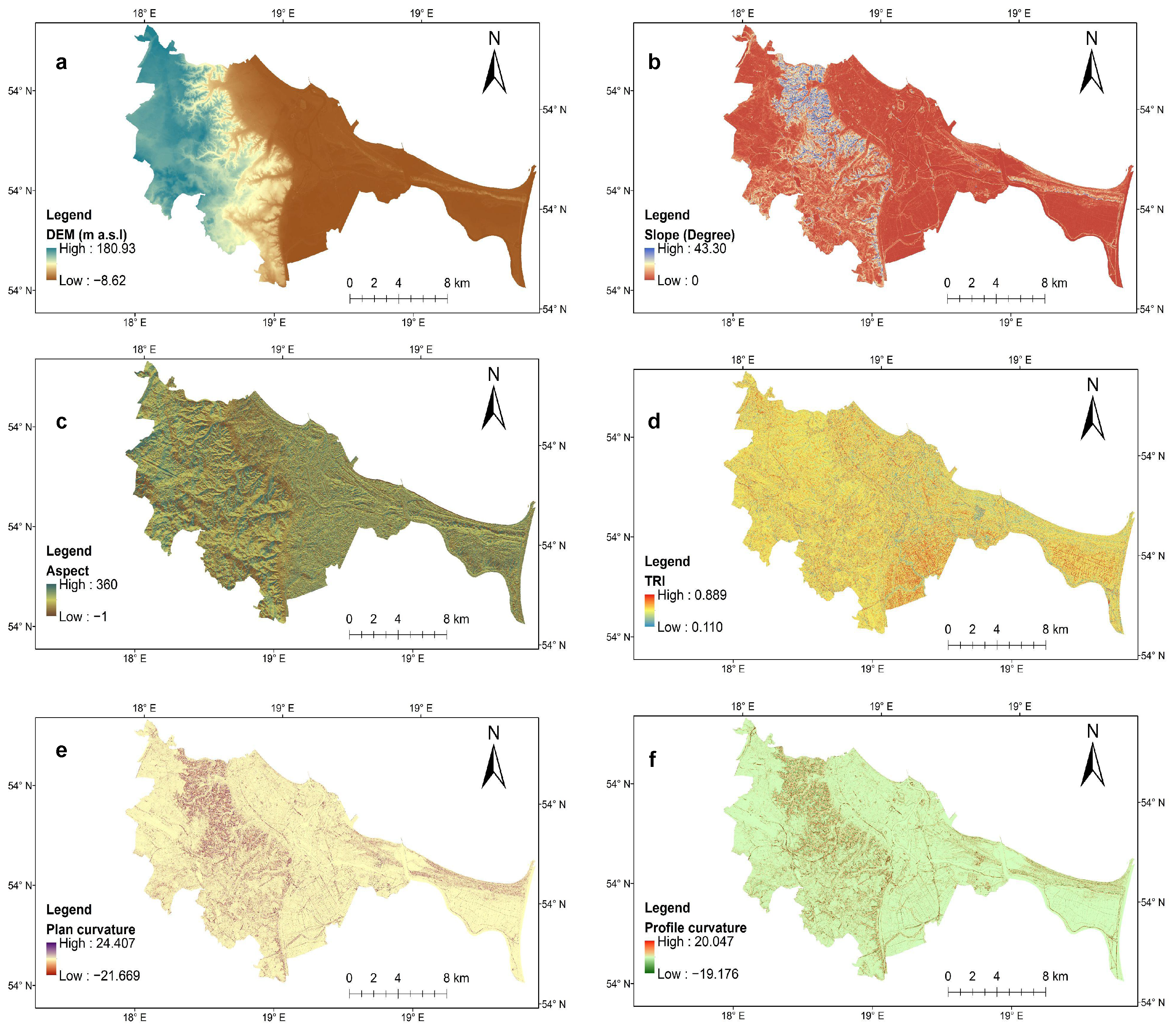
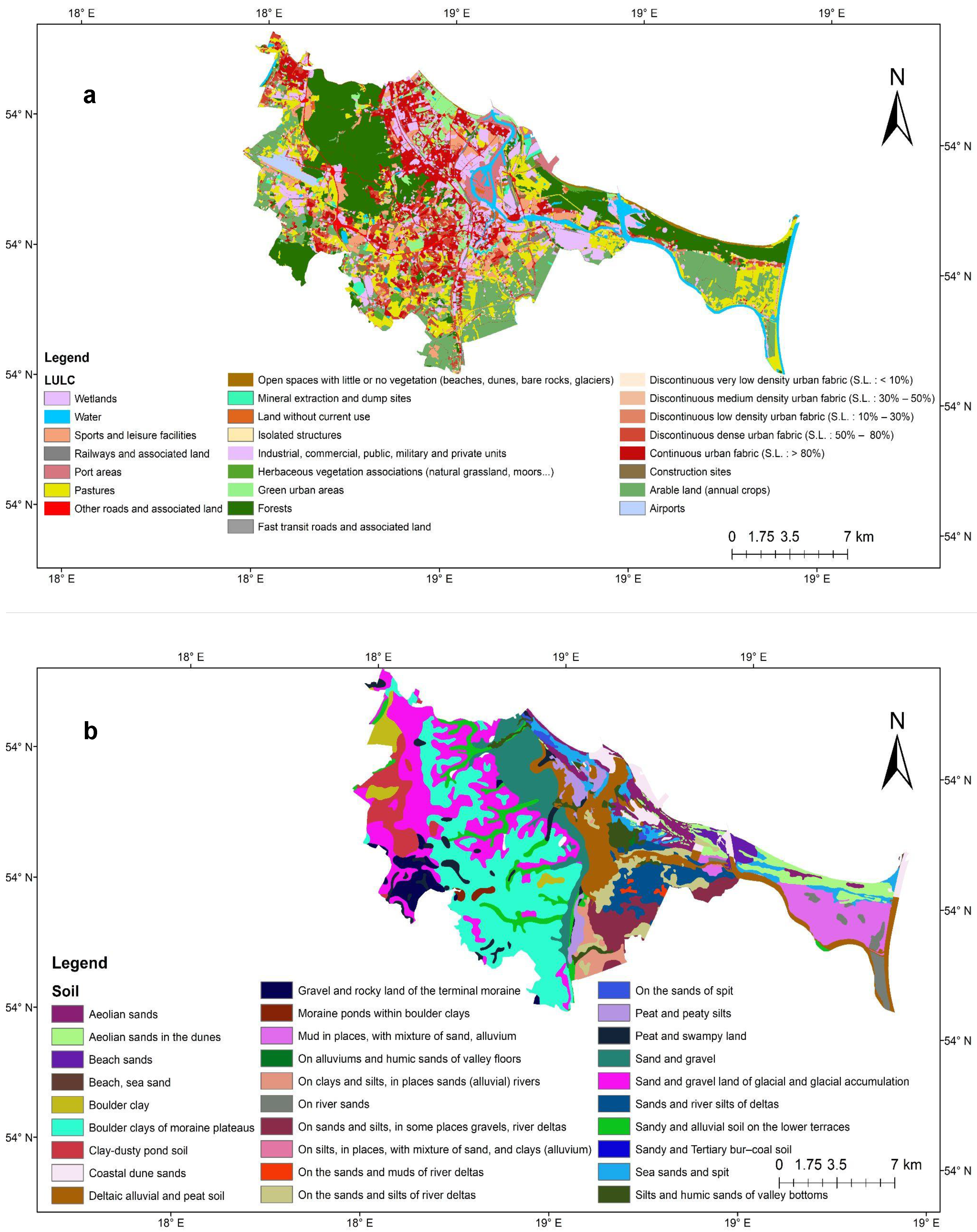
3.1. Flood Factor Maps

Factor values for flood and non-flood sites were extracted to train, test, and predict flood susceptibility. The histograms (Figure 3) represent the factors’ frequency distributions with Kernel Density Estimate (KDE) curves, representing historical flood locations in the study area. The x-axis shows the values of each variable for historical flood locations, while the y-axis shows their frequency in the dataset.

Figure 3. Histograms and overlaid kernel density estimates illustrating the distribution of key features that are critical for flood susceptibility analyses at historical flood sites.

Slope: The slope distribution is skewed towards lower values with a long tail extending towards higher values (Figure 3). Most historical flooded areas have a gentler slope, with fewer steep slopes (Figure A1b in Appendix A). Steep slopes hinder infiltration and increase runoff, causing flooding [22].

DEM: DEM is skewed towards lower elevations. The DEM map of Gdańsk shows elevation from below sea level (−8 m) to higher terrain (up to 180 m) in the southern and southwestern parts (Figure A1a). This topographic variation divides Gdańsk into three areas: the upper terrace, the lower terrace, and the edge zone. Lower terraces, including the coastal belt, are vulnerable to sea level rises and flooding [57].

LST: Gdańsk’s temperature ranged from $8.3$ °C and $36.7$ °C, with higher temperatures in urban areas, industrial clusters and agricultural land on the eastern and southwestern sides (Figure A2e). The LST distribution shows a central tendency, indicating an optimal temperature range where flood-related processes or human activity influencing flood susceptibility are more prevalent. In contrast, lower temperatures are associated with the rural areas, green spaces, and forests of Gdańsk. LST is critical in flood susceptibility studies, as high temperatures and increased impervious surfaces contribute to runoff and flood hazards [41].

River buffer: Distance from the river histogram shows a bimodal distribution (Figure 3), with peaks at both the low and high ends. This shows that historical flood locations are either very close to rivers or far from rivers (Figure A2g). Areas near rivers are more susceptible to flooding, especially during heavy rainfall.

Rainwater collectors: In Gdańsk, the role of rainwater collectors depends on the weather conditions and infrastructure capacity. Collectors quickly channel water downhill on steep slopes, reducing accumulation and pressure points. However, in low-lying areas, collectors must handle runoff from upstream basins. If the rainwater surpasses the collectors’ capacity during heavy rainfall, the overflow can cause nearby flooding. Additionally, rising sea levels can cause backflow into collectors, reducing their capacity to manage runoff and increasing floods. Higher sea levels also reduce the hydraulic gradient within the collectors, decreasing their capacity to handle runoff. Proximity to rainwater collectors, as shown on the map (Figure A2h), is a crucial indicator of flood susceptibility, particularly during periods of intense precipitation or when sea levels rise.

Soil: Soil distribution shows multiple peaks, indicating varied soil types at flood locations, ranging from sandy, sandy gravel, and alluvial soil on lower terraces (Figure A3b). The descriptive soil types in the map (Figure A3b) are tied to specific ranges of numerical values (Figure 3), which allows for the mapping of spatial variation in soil characteristics.

NDVI: NDVI has a bell-shaped distribution centred at around 0.2, indicating moderate vegetation cover in most areas. Vegetation and soil can influence infiltration, soil erosion, and water retention, all affecting flooding [11].

LULC: The LULC map of Gdańsk (Figure A3a) is divided into urban fabric, agricultural land, forests, water bodies, and more. The LULC histogram (Figure 3) shows numerical values with multiple peaks, reflecting diverse land use types (e.g., urban, forest, agriculture). Each range of values represents a specific LULC class, connecting the numerical data to the land use and land cover types displayed on the map (Figure A3a). Significant peaks representing historical flood points are found in continuous urban fabric, road networks, and industrial and commercial land. Specific land use types can significantly impact water runoff and absorption, which are critical factors in flood dynamics [58]. The LULC map shows urban expansion towards the south and southwest of Gdańsk, correlating directly with LST.

In addition, features with broader value ranges provide distinct information for predictive modelling (flood vs. non-flood). For instance, slope and DEM are primarily clustered at lower values, contrasting with LST, NDVI, soil, and LULC, which display a wider distribution. This suggests that slope and DEM values in historical flood zones remain consistent over time in Gdańsk, potentially limiting their effectiveness in predicting flood-susceptible areas compared to other selected features.

The flood factor analysis shows that each factor uniquely impacts flood susceptibility, depending on its distribution patterns. This insight is essential to effectively identifying and mitigating floods in Gdansk.

3.2. Multicollinearity of Factors

Multicollinearity among 16 factors was assessed (Table 3). The minimum VIF value (1.03) was for the aspect, and the maximum (3.36) was for the slope. All features had VIF values of less than 5, indicating negligible collinearity or independence from each other. Hence, all of these factors were suitable for further processing.

Table 3. Multicollinearity analysis showing VIF values of less than five for all the factors of flood susceptibility.

Variables	VIF	Variables	VIF
LST	2.23	Coastal buffer	1.46
Aspect	1.03	Soil	1.98
Slope	3.36	DEM	1.86
Plan curvature	1.57	NDWI	1.92
Profile curvature	1.65	SPI	2.60
NDVI	2.04	LULC	1.20
TRI	1.25	TWI	2.40
River buffer	1.15	Rainwater collectors	1.42

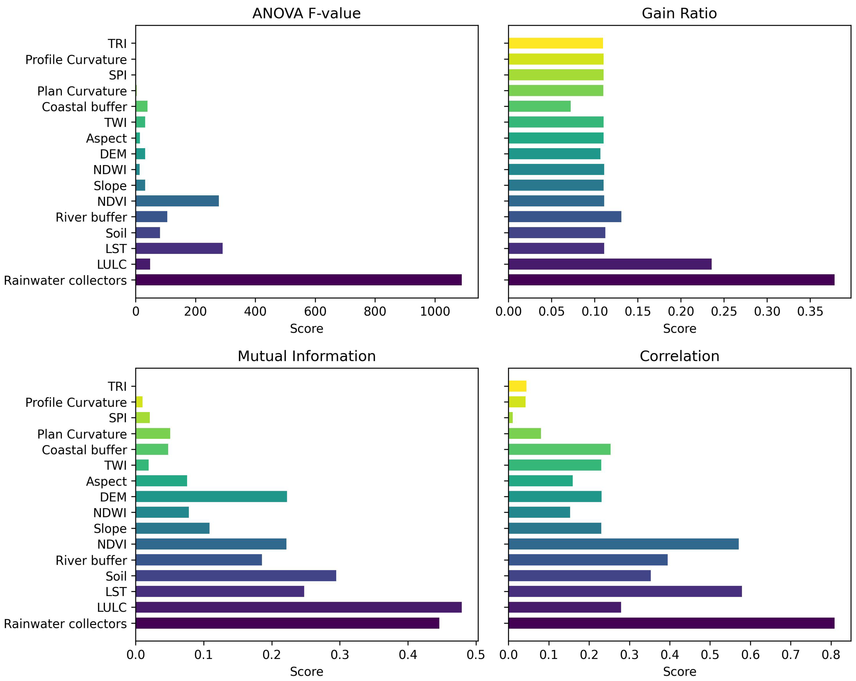
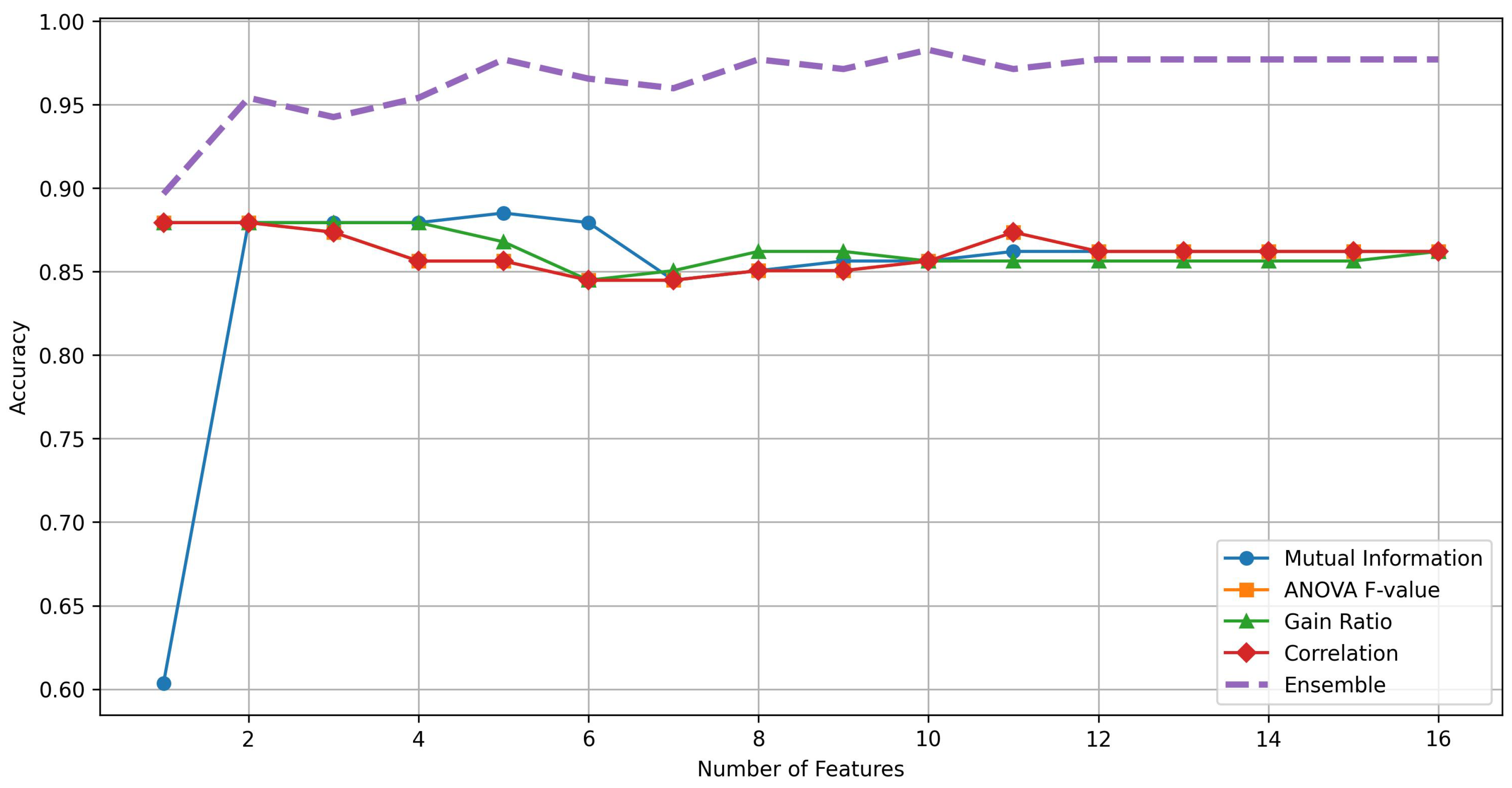
3.3. Ensemble Feature Selection

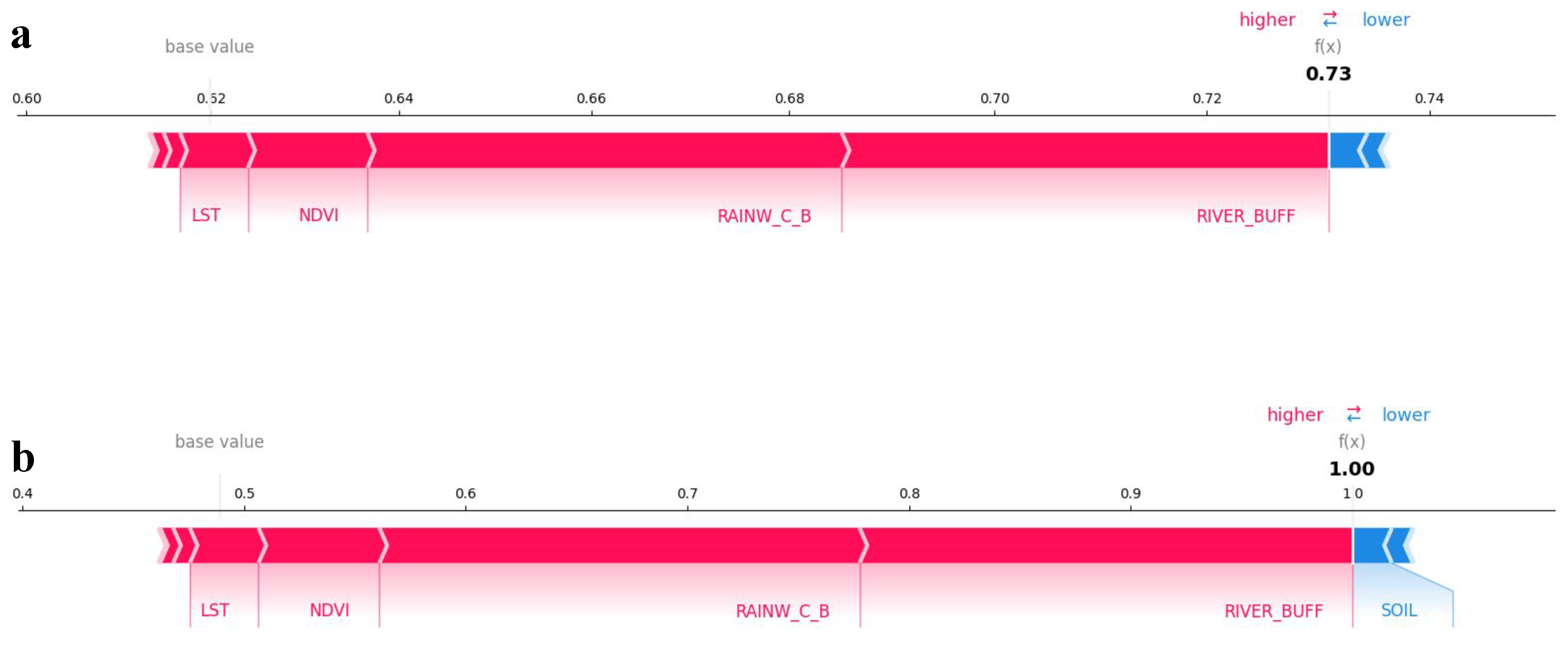
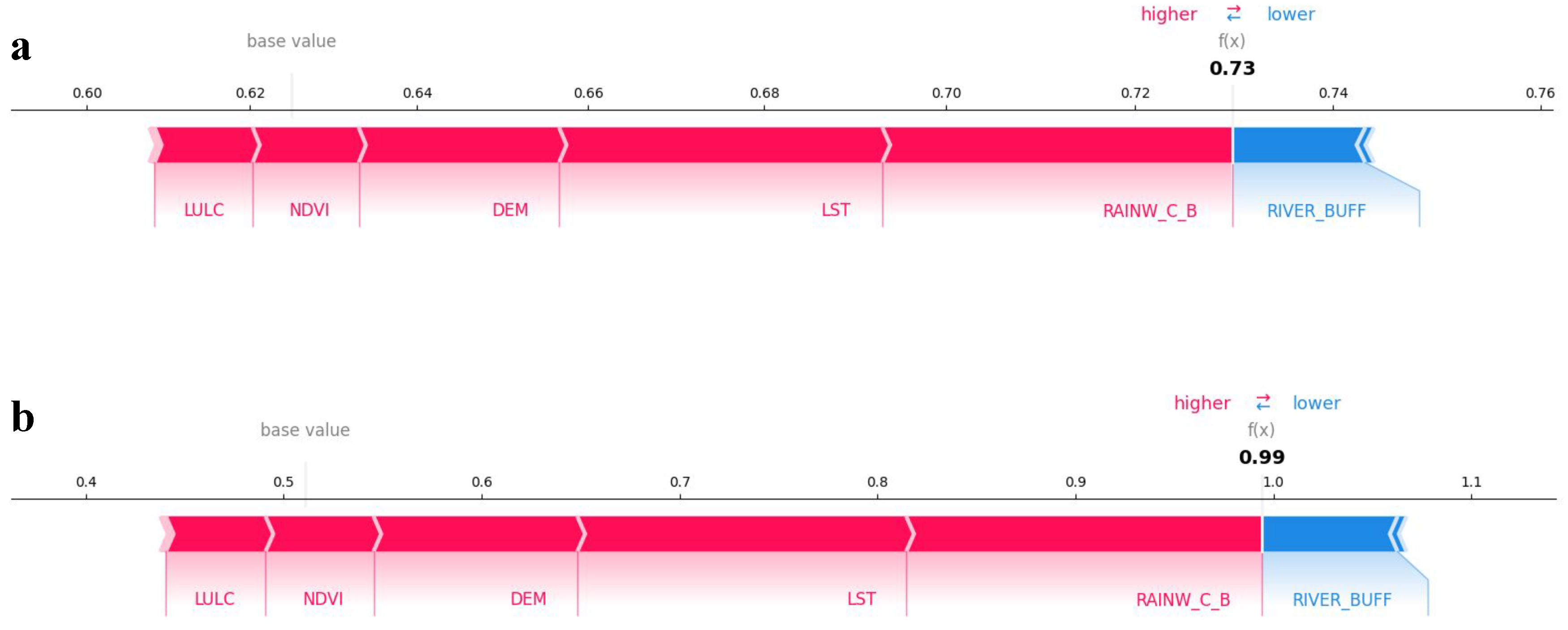
The choice of factors affects machine learning models’ accuracy, either directly or indirectly, but selecting and categorising appropriate factors is challenging without a universal rule. Therefore, ensemble feature selection identified the most significant factors from the dataset. Feature selection began with various filter methods, each using distinct ranking algorithms.

Figure 4 shows the outcome of feature selection, highlighting features’ recurrence patterns in predicting flood susceptibility. Key factors such as LULC, proximity to rainwater collectors, Land Surface Temperature (LST), buffer zones around rivers, soil composition, and NDVI consistently appeared as top features across all filter methods. In contrast, features like TRI, SPI, and profile and plan curvature showed less consistent rankings, suggesting lower significance or a more nuanced relationship with the target variable that is not easily quantifiable or linear.

Figure 4. Comparative analysis of feature rankings using four filter methods: ANOVA-F, gain ratio, mutual information, and correlation.

ANOVA F-value, Mutual Information, Gain Ratio, and Correlation metrics offer varied perspectives while collectively reinforcing specific features’ significance. Therefore, the rankings obtained from these methods served as the basis for the EFFS method, which aims to eliminate irrelevant or redundant features.

Figure 5 illustrates a trend where accuracy initially rises (88%) when features increase from 2 to 6. Hence, a minimal feature set is inadequate for recognising the complexity of the data. Beyond this point, accuracy stabilises at 86% across four selection methods. It also slightly decreases, suggesting an optimal subset of features that balances model complexity and performance. A similar finding in a flood susceptibility study indicated that adding more factors may not necessarily improve model effectiveness [22].

Figure 5. Accuracy of ML classifier using different feature selection methods and EFFS.

Ensemble feature selection outperforms individual methods across all feature sizes. Initially, accuracy increases to 95% and peaks at around ten features. High accuracy (98%) is maintained across all subsequent feature sizes, implying that redundant features in the original dataset contribute minimally or not at all to class identification. This finding aligns with studies in cloud computing and human activity recognition, where ensemble feature selection outperformed individual approaches using fewer features [25,28]. Therefore, EFFS emerges as a compelling approach for the selection of an optimal feature set, maximising classifier accuracy while maintaining computational efficiency. This efficiency is crucial for large-scale flood susceptibility assessments.

Table 4 outlines the top 10 attributes identified by the EFFS method as having a strong influence on flood susceptibility. These features will be the primary input variables when developing predictive models for future flood events, leading to more reliable maps that can better inform flood management strategies. While the factors influencing flood occurrence vary across regions [22], the significance of these factors is context-specific and dependent on the dataset and the characteristics of the study area. Therefore, the findings may not be universally generalisable, and excluding certain factors does not negate their potential impact on flooding.

Table 4. Features selected by the ensemble-based filter feature selection method.

Filter Method	Selected Features
EFFS	Rainwater collectors, LULC, LST, soil, river buffer, NDVI, slope, NDWI, DEM, aspect

3.4. Explainability

SHAP explained the outcomes of the models selected for this study. The individual SHAP force plot shows the interactions between variables when reaching the predicted target variable [24]. Force plots (Figure 6) have three key characteristics: (i) output value, the predicted value for an individual observation; (ii) base value, the average prediction across the test dataset; and (iii) colors, where red variables push the prediction higher and blue variables push it lower.

Figure 6. SHAP force plots for flood instances, showing the contribution of key features: (a) Contribution of key features for flood instance 1. (b) Contribution of key features for flood instance 2.

Figure 6a shows a flood susceptibility instance where the model predicts a high flood probability of 0.73. Features like river buffer, rainwater collectors, LST, DEM, and NDVI significantly push the prediction toward the flood. In another instance (Figure 6b), the model predicts a maximum flood probability of 1.00. Features like river buffers, rainwater collectors, LST, and NDVI strongly influence the model towards predicting floods, indicating their critical role in the model’s decision-making process. Soil contributes negatively but is overshadowed by the positive contributions.

In this instance (Figure 7a), the model predicts a high flood probability of 0.73, implying a lower likelihood of non-flood. Features like LULC, rainwater collectors, LST, DEM, and NDVI contribute positively towards flood prediction (and negatively towards non-flood prediction). The river buffer slightly increases the non-flood probability, but its impact is much less significant than that of the other features. In another instance (Figure 7b), the model predicts a very high flood probability of 0.99, implying a very low likelihood of non-flood. Features such as rainwater collectors, LST, DEM, NDVI, and LULC firmly push the prediction toward flood (away from non-flood). Similar to plot (a), the negative contribution of the river buffer is minimal compared to the positive influences of the other features.

Figure 7. SHAP force plots for non-flood instances, showing the contribution of key features: (a) Contribution of key features for non-flood instance 1. (b) Contribution of key features for non-flood instance 2.

These interpretations underscore the varying influence of features across different instances, highlighting the importance of rainwater collectors, LST, NDVI, and river buffers in flood prediction. Understanding these feature contributions can refine the model’s performance and enhance interpretability in flood prediction systems.

Figure 8 shows SHAP summary plot values for flood factors, ranking their importance in the model’s predictions from most impactful, at the top, to least impactful, at the bottom. Each point on the plot represents the SHAP value, and its position on the x-axis indicates its impact on the model predictions. An SHAP value of zero means it has no impact, while values’ position to the right or left of the graph suggest higher or lower impacts.

Figure 8. Explanation of models’ (a) SVM, (b) RF, and (c) ANN using SHAP. A cluster of data around the SHAP value of zero indicates a small impact on model output.

For a classification task, SHAP value > 0 increases the likelihood of a class, while SHAP value < 0 decreases the probability. The colours on the plot represent feature values, with cooler colours representing lower values and warmer colours representing higher values or binary class indications. The spread of the points represents the variability of the features’ impact; a wide spread suggests varied effects, while a narrow spread indicates a more consistent impact.

Rainwater collectors, LST, DEM, soil, river buffer, and NDVI strongly impact the model predictions, while other factors are mostly centered around zero or have a slightly positive or negative impact. This finding is also supported by the results of EFFS and individual feature selection methods, as shown in Figure 4. Recent studies have demonstrated that explainable models significantly enhance the understanding of model outcomes [17,24,31,56]. Hence, SHAP values help validate the model by confirming that the most influential features align with known flood susceptibility factors, such as elevation [11,21,22], slope [21], river network, and land cover [13,21,22].

In the SHAP value graph of ANN (Figure 8), features like rainwater collectors and LST show high SHAP values, suggesting that these variables strongly influence the model’s predictions. By showing the impact of each feature, stakeholders can better understand the factors driving flood hazards in their regions, facilitating more informed decision-making.

On the map, areas with dense rainwater collector networks or a higher LST (Figure A2e) correspond to regions marked as highly or very highly susceptible areas, indicating that these features potentially escalate the flood hazard in these zones. Furthermore, zones closer to rivers are designated high-hazard areas due to the potential overflow or concentrated runoff during heavy rains. Enhanced explainability makes flood susceptibility maps more understandable and accurate by helping to communicate risks to the public and policymakers.

3.5. Performance of Flood Prediction

After training, the models were evaluated using statistical measures and ROC curves for training and testing data to assess model fit and generalisation. Table 5 presents the results.

Table 5. Performance evaluation of models for training and testing datasets using statistical measures.

Methods	SVM			RF			ANN
	Training	Testing		Training	Testing		Training	Testing
RMSE	0.270	0.330		0.260	0.252		0.073	0.168
MAE	0.133	0.160		0.182	0.151		0.016	0.057
Accuracy	0.905	0.862		0.903	0.913		0.992	0.965
AUC	0.972	0.960		0.965	0.974		0.999	0.994
Sensitivity	0.907	0.892		0.855	0.964		0.989	0.988
Specificity	0.904	0.833		0.947	0.867		0.995	0.944

The RMSE and MAE values for the training datasets are 0.073, 0.016 for ANN, 0.260, 0.182 for RF, and 0.270, 0.133 for SVM, with the fewest errors being obtained using the ANN model. Similar results were observed for the testing data: ANN (RMSE: 0.168, MAE: 0.057), RF (RMSE: 0.252, MAE: 0.151), and SVM (RMSE: 0.330, MAE: 0.160). ANN achieved an accuracy of 0.992 for training and 0.965 for testing, correctly classifying 96% of pixels as flood and non-flood in the test dataset. RF followed, with an accuracy of 0.903 and 0.913, and SVM, with an accuracy of 0.905 and 0.862.

The flood maps produced by the three models were validated using AUROC for training and testing datasets. The success rate curve for the training data (Figure 9) shows the ANN model to have the highest AUC (0.999), followed by SVM (AUC = 0.972) and RF (AUC = 0.965). The prediction rate curve for the validation dataset (Figure 9) showed similar results: ANN (AUC = 0.994), RF (AUC = 0.974), and SVM (AUC = 0.960).

Figure 9. ROC curves for training and test datasets for SVM, RF, and ANN under best parameter configuration.

The performance difference between the training and testing datasets is a common occurrence in machine learning, often attributed to model generalisation [59]. In this case, the models performed slightly poorer using the testing dataset compared to the training dataset, as evidenced by the higher RMSE and lower accuracy in testing for all models.

This discrepancy likely arises because the models are trained on a specific set of data, allowing them to learn intricate patterns within the training set. However, when applied to new, unseen testing data, the models may struggle to generalise as well, especially if the testing data contain variability that is not fully captured in the training set. This slight performance drop reflects the models’ ability to generalise to new scenarios rather than overfitting the training data [10].

Additionally, ANN’s complexity may contribute to its better performance due to its ability to capture more complex patterns. At the same time, simpler models like SVM and RF show greater discrepancies between the training and testing results. However, the overall differences remain small, suggesting that all models were reasonably effective in predicting flood hazard across both datasets.

3.6. Flood Susceptibility Maps

Models were trained using hyperparameter tuning for optimal performance. The RBF kernel with a C value of 0.1 for SVM showed the best performance, with an RMSE of 0.270. Previous research also found the RBF kernel to be superior for determining flood susceptibility [11,13,60]. ANN was tested with various neurons and hidden layers, and the best configuration had four hidden layers, offering the highest accuracy and lowest RMSE (Table 2).

Each pixel in the flood susceptibility map is assigned a value between 0 and 1, indicating flood probability, with 0 meaning no probability and one meaning 100% probability [22]. The probability values must be classified into various classes to create visually effective susceptibility maps. Quantile, natural breaks, equal intervals, and standard deviations can be used [61]. In this study, the final maps were divided into five classes using quantile classification, ensuring each class contained an equal number of pixels.

Classifiers were categorised into five susceptibility levels: very low. (0.01–0.22), low (0.22–0.39), moderate (0.39–0.57), high (0.57–0.75), and very high (0.75–0.98). Table 6 shows the percentage of the area in each class for each classifier. The ANN model indicated that 36.601% of the region falls under very high susceptibility and 24.144% under high susceptibility, totalling 60.745% in the high-susceptibility zone (Figure 10). For RF, 29.810% is very high, and 27.652% is high, while for SVM, 41.803% of the area comes under the very high-susceptibility class, and 10.302% comes under the high susceptibility class. Low- and very low-susceptibility areas together comprise 39.883% (SVM), 24.915% (RF), and 28.368% (ANN).

Table 6. Flood susceptibility classification using the SVM, RF, and ANN models.

Class	SVM (%)	RF (%)	ANN (%)
Very low	17.686	6.151	9.709
Low	22.197	18.764	18.659
Medium	8.013	17.624	10.886
High	10.302	27.652	24.144
Very High	41.803	29.810	36.601

Figure 10. Flood susceptibility maps for SVM, RF, and ANN models.

The analysis showed that high- and very high-flood-susceptibility regions are found in the central and northwestern parts of Gdańsk, correlating with fire brigade interventions after heavy rainfall. Figure 11 shows the flood distribution per district, with colour intensity indicating the number of flood events. Wrzeszcz Górny, Wrzeszcz Dolny, Osowa, Śródmieście, Oliwa, and Orunia had the most interventions [36], as shown in Figure 11. Highly susceptible areas are found near rainwater collectors and watercourses, especially near the edge zone and the lower terrace. Densely built and flat regions receive runoff from the upper terrace during heavy rainfall. The Historic Center of Gdańsk, located in this lower terrace area, is also prone to flooding [37], suggesting that rainwater collectors and watercourses struggle to manage runoff effectively under extreme rainfall events [35]. The main areas that are vulnerable to flash floods in Gdańsk are divided into three regions: (1) the moraine hills (upper terrace), subdivided into plateau and slopes, (2) the polders, and (3) Canal Radunia.

Figure 11. Flash flood-susceptible areas in Gdańsk; the top map shows the LULC with upper and lower terraces; the lower section features satellite images of specific areas (A–D), and a map indicating flood distribution across different districts, with colour gradients representing the number of floods.

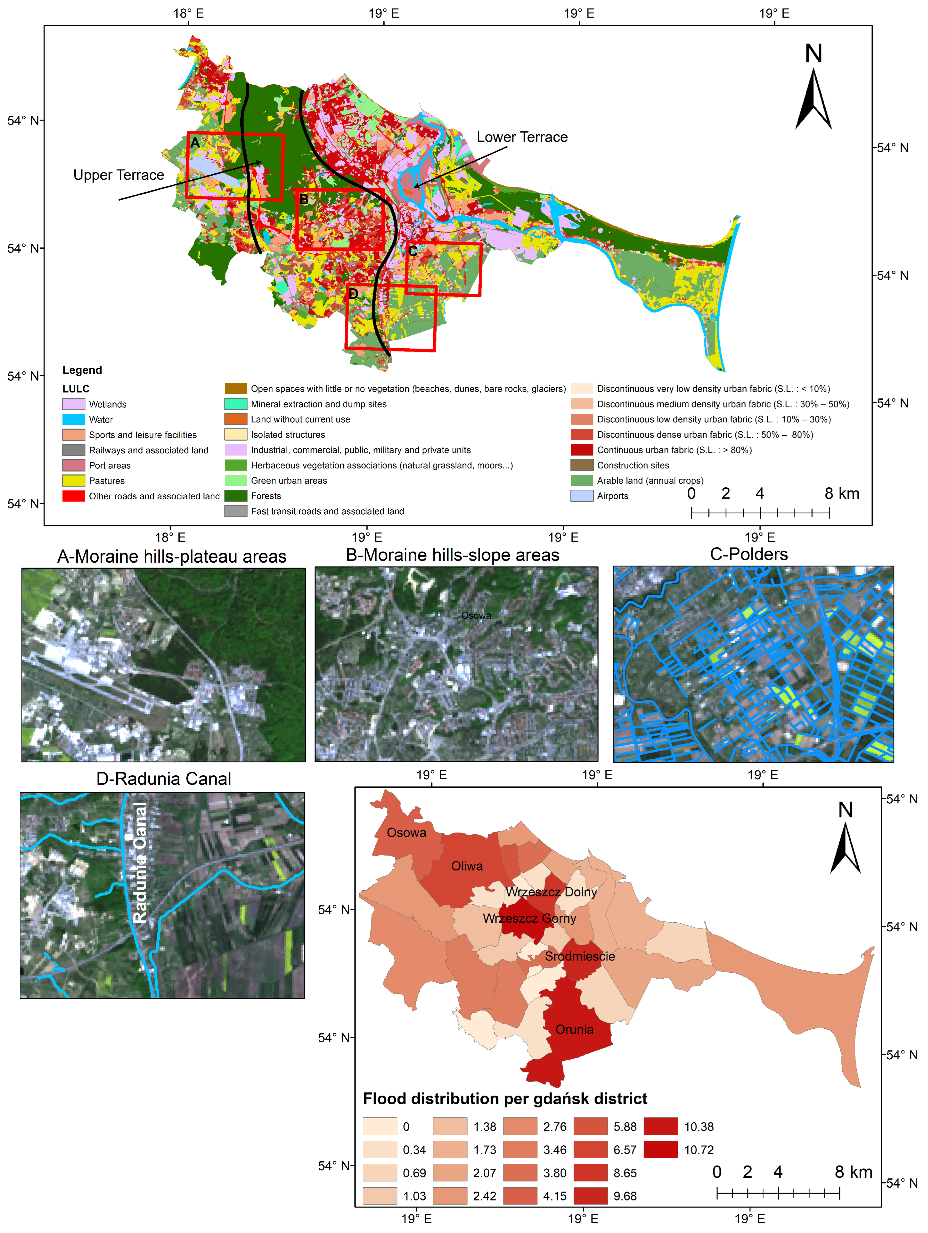
• The plateau (Figure 11A) of Gdańsk moraine hills is less urbanised, with gentler slopes, leading to slower runoff. Increased urbanisation poses a threat by potentially raising peak flow during rainfall, surpassing the existing retention basins’ capacity. To address this, Gdańsk has implemented strict regulations [34], pausing some development plans, although enforcement varies by region. If urban expansion is managed or its impacts are mitigated, the need for urgent intervention on the plateau may be minimal [33].
• The moraine hills with slopes (Figure 11B) in southwest Gdańsk are increasingly urbanised and prone to flash floods due to their steep terrain, heavy rainfall, and urbanisation. Unlike low-lying areas, they are not vulnerable to storm surges because of their higher elevation. Urbanisation has stressed the water system, replacing natural ecosystems with an infrastructure that accelerates runoff and strains old sewage systems. The storm drainage network and impermeable surfaces direct water into waterways like the Radunia Canal, overwhelming their capacity and exacerbating flooding [35]. Retention basins are crucial in reducing peak flows in these hills [34]. Many basins have already been constructed, with more planned, mainly on the plateau. However, the rising land costs in this area diminish the cost-effectiveness of these measures [33]. Another measure is retaining up to 30 mm of rainwater in new developments [5].
• The rural zone, particularly the polder area southeast of the city (Figure 11C), is well-prepared for water-related challenges. Initially designed for agriculture with controlled water-level regulation, it has a sufficient buffering capacity to manage short, intense rainfalls without significant impact. Although flooding occurred in 2001 when Canal Radunia’s capacity was exceeded, overall, the polder’s drainage system effectively handles water flow. Rainfall–runoff in the polders poses no significant issues, making them a viable option for development compared to the moraine hills. However, enhancing the polder’s drainage and pumping systems would be necessary to accommodate the increased runoff from urbanised surfaces [33].
• Canal Radunia, an artificial channel dating back to the Middle Ages designed to drain the polder and supply water to Gdańsk, receives water from small natural streams in the moraine hills and has a maximum discharge capacity of 20 ${\mathrm{m}}^3/\mathrm{s}$. During the 2001 flash flood, the canal was overwhelmed by a combined discharge of around 100 ${\mathrm{m}}^3/\mathrm{s}$ from streams, stormwater, and overland flow, resulting in breaches at five places and subsequent flooding east of the channel [4,33]. Gdańsk implemented a comprehensive three-stage rainwater management strategy involving on-site water management, municipal stormwater systems, retention reservoirs, and crisis response measures. Gdańsk has engaged residents in climate change adaptation measures through social platforms, citizens’ panels, and the Gdańsk Climate Change Forum, fostering knowledge-sharing about pluvial flood mitigation [5].

4. Limitations and Future Research Directions

Gdańsk faces greater challenges from flash floods coinciding with storm surges and sea level rises, threatening local beaches and aquifers. Combined with climate change-induced storm events, these pose substantial risks to the city. Future research should further refine flood models, particularly to address sea level rises and climate change impacts.

A key limitation of this study is that it used a single model across Gdańsk’s varied topography. Flash flood-prone areas differ from those vulnerable to sea level rises, as illustrated by the distinct zones on the study area map (Figure 2). Future research should focus on developing and refining separate predictive models tailored to these hazards. Coastal flooding models must be calibrated for low-lying areas susceptible to sea level rises. This approach will enhance the accuracy and relevance of flood susceptibility assessments in urban planning and climate adaptation strategies for Gdańsk.

The study relies on historical flood data, remote sensing, and other geospatial datasets, which may only sometimes be fully comprehensive or up to date. Future research could benefit from integrating higher-resolution data or real-time monitoring systems for more precise flood prediction. Additionally, while SHAP improves model interpretability, complex models like ANN tend to be less interpretable compared to simpler models. This trade-off between model accuracy and interpretability could be a limitation for decision-makers who prefer clearer, more transparent models.

5. Conclusions

Flood susceptibility mapping in Gdańsk, Poland, employing SVM, RF, and ANN models, ensemble-based filter feature selection, and explainability techniques, provided valuable insights into flood susceptibility. The study draws several conclusions:

• Ensemble feature selection identified critical factors influencing flood susceptibility in Gdańsk, including LULC, proximity to rainwater collectors, LST, river buffer zones, soil composition, and NDVI. These factors were consistently highlighted across multiple feature selection methods as pivotal in predicting flood-prone areas.
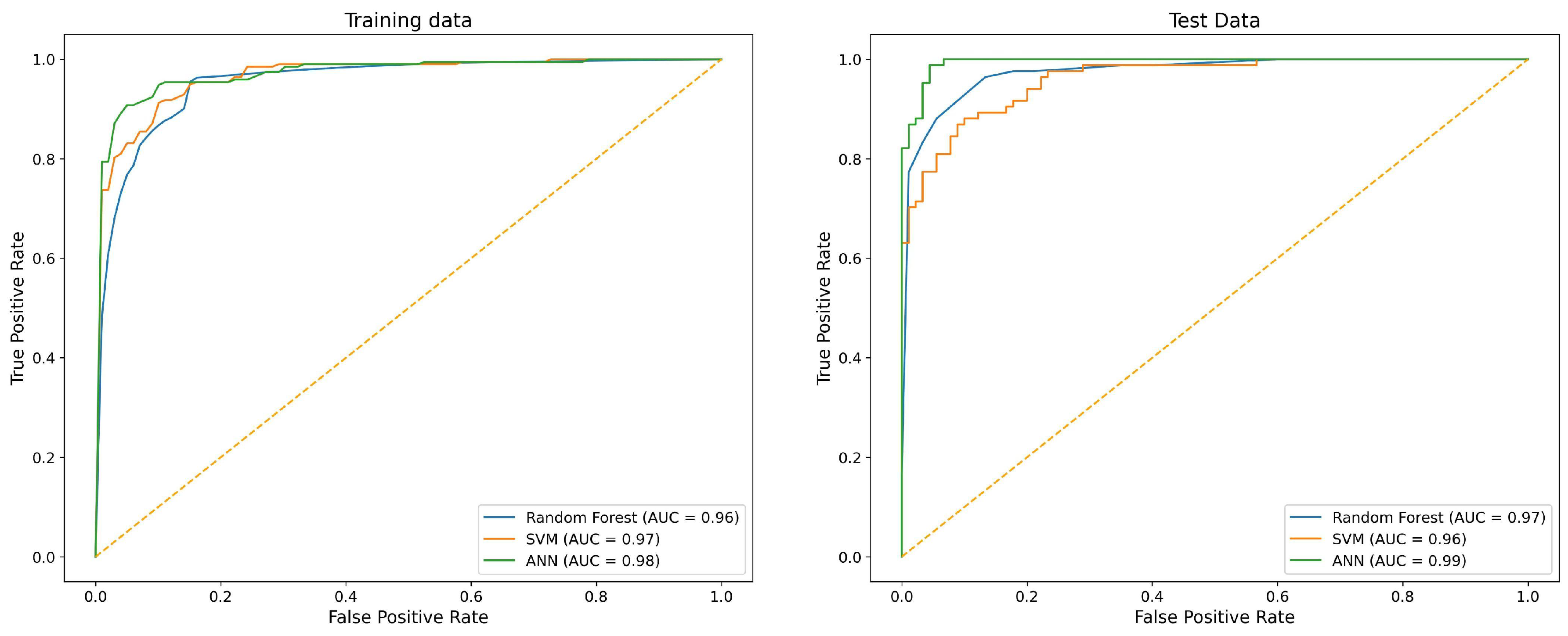
• The predictive performance of the SVM, RF, and ANN models was evaluated using AUC, with the ANN model demonstrating a superior performance (AUC 0.992) compared to RF (AUC 0.965) and SVM (AUC 0.905), underscoring the efficacy of machine learning approaches in accurately delineating flood susceptibility zones in Gdańsk.
• To tackle the issue of model interpretability, SHAP clarified the impact of specific features on model predictions. This approach improves transparency by providing insights into how particular factors (rainwater collectors, LST, NDVI, river buffer) contribute to flood susceptibility assessments and facilitating informed decision-making in flood mitigation strategies.
• Future research should focus on creating separate prediction models considering floods associated with sea level rises and climate change.
• Urban planners, policymakers, and disaster management authorities can prioritise interventions and distribute resources effectively using the practical insights from this study. Using machine learning techniques and geospatial data, stakeholders can anticipate flood hazards and improve community resilience.

References

- Ionita, M.; Nagavciuc, V.; Guan, B. Rivers in the sky, flooding on the ground: The role of atmospheric rivers in inland flooding in central Europe. Hydrol. Earth Syst. Sci. 2020, 24, 5125–5147. [Google Scholar] [CrossRef]
- Mrozik, K.D. Problems of local flooding in functional urban areas in Poland. Water 2022, 14, 2453. [Google Scholar] [CrossRef]
- Konieczny, R.; Pińskwar, I.; Kundzewicz, Z. The September 2017 flood in Elblag (Poland) in perspective. Meteorol. Hydrol. Water Manag. Res. Oper. Appl. 2018, 6, 67–78. [Google Scholar] [CrossRef]
- Majewski, W. Urban flash flood in Gdańsk–2001. Case Study Meteorolology Hydrol. Water Manag. 2016, 4, 41–49. [Google Scholar] [CrossRef]
- Szydłowski, M.; Gulshad, K.; Mustafa, A.M.; Szpakowski, W. The impact of hydrological research, municipal authorities, and residents on rainwater management in Gdańsk (Poland) in the process of adapting the city to climate change. Acta Sci. Pol. Form. Circumiectus 2023, 22, 59–71. [Google Scholar] [CrossRef]
- Pińskwar, I.; Choryński, A.; Graczyk, D. Risk of Flash Floods in Urban and Rural Municipalities Triggered by Intense Precipitation in Wielkopolska of Poland. Int. J. Disaster Risk Sci. 2023, 14, 440–457. [Google Scholar] [CrossRef]
- Ahmadlou, M.; Karimi, M.; Alizadeh, S.; Shirzadi, A.; Parvinnejhad, D.; Shahabi, H.; Panahi, M. Flood susceptibility assessment using integration of adaptive network-based fuzzy inference system (ANFIS) and biogeography-based optimization (BBO) and BAT algorithms (BA). Geocarto Int. 2019, 34, 1252–1272. [Google Scholar] [CrossRef]
- Khosravi, K.; Pham, B.T.; Chapi, K.; Shirzadi, A.; Shahabi, H.; Revhaug, I.; Prakash, I.; Bui, D.T. A comparative assessment of decision trees algorithms for flash flood susceptibility modeling at Haraz watershed, northern Iran. Sci. Total Environ. 2018, 627, 744–755. [Google Scholar] [CrossRef]
- Kaya, C.M.; Derin, L. Parameters and methods used in flood susceptibility mapping: A review. J. Water Clim. Chang. 2023, 14, 1935–1960. [Google Scholar] [CrossRef]
- Islam, A.R.M.T.; Talukdar, S.; Mahato, S.; Kundu, S.; Eibek, K.U.; Pham, Q.B.; Kuriqi, A.; Linh, N.T.T. Flood susceptibility modelling using advanced ensemble machine learning models. Geosci. Front. 2021, 12, 101075. [Google Scholar] [CrossRef]
- Yaseen, A.; Lu, J.; Chen, X. Flood susceptibility mapping in an arid region of Pakistan through ensemble machine learning model. Stoch. Environ. Res. Risk Assess. 2022, 36, 3041–3061. [Google Scholar] [CrossRef]
- Parvin, F.; Ali, S.A.; Calka, B.; Bielecka, E.; Linh, N.T.T.; Pham, Q.B. Urban flood vulnerability assessment in a densely urbanized city using multi-factor analysis and machine learning algorithms. Theor. Appl. Climatol. 2022, 149, 639–659. [Google Scholar] [CrossRef]
- Tehrany, M.S.; Pradhan, B.; Jebur, M.N. Flood susceptibility analysis and its verification using a novel ensemble support vector machine and frequency ratio method. Stoch. Environ. Res. Risk Assess. 2015, 29, 1149–1165. [Google Scholar] [CrossRef]
- Khosravi, K.; Nohani, E.; Maroufinia, E.; Pourghasemi, H.R. A GIS-based flood susceptibility assessment and its mapping in Iran: A comparison between frequency ratio and weights-of-evidence bivariate statistical models with multi-criteria decision-making technique. Nat. Hazards 2016, 83, 947–987. [Google Scholar] [CrossRef]
- Kolerski, T.; Kalinowska, D. Mathematical modeling of flood management system in the city of Gdańsk, Oruński stream case study. Acta Sci. Pol. Form. Circumiectus 2019, 18, 63–74. [Google Scholar] [CrossRef]
- Paprotny, D.; Vousdoukas, M.I.; Morales-Nápoles, O.; Jonkman, S.N.; Feyen, L. Pan-European hydrodynamic models and their ability to identify compound floods. Nat. Hazards 2020, 101, 933–957. [Google Scholar] [CrossRef]
- Pradhan, B.; Lee, S.; Dikshit, A.; Kim, H. Spatial flood susceptibility mapping using an explainable artificial intelligence (XAI) model. Geosci. Front. 2023, 14, 101625. [Google Scholar] [CrossRef]
- Rahman, M.; Ningsheng, C.; Islam, M.M.; Dewan, A.; Iqbal, J.; Washakh, R.M.A.; Shufeng, T. Flood susceptibility assessment in Bangladesh using machine learning and multi-criteria decision analysis. Earth Syst. Environ. 2019, 3, 585–601. [Google Scholar] [CrossRef]
- Shafizadeh-Moghadam, H.; Valavi, R.; Shahabi, H.; Chapi, K.; Shirzadi, A. Novel forecasting approaches using combination of machine learning and statistical models for flood susceptibility mapping. J. Environ. Manag. 2018, 217, 1–11. [Google Scholar] [CrossRef]
- Ngo, P.T.T.; Hoang, N.D.; Pradhan, B.; Nguyen, Q.K.; Tran, X.T.; Nguyen, Q.M.; Nguyen, V.N.; Samui, P.; Tien Bui, D. A novel hybrid swarm optimized multilayer neural network for spatial prediction of flash floods in tropical areas using sentinel-1 SAR imagery and geospatial data. Sensors 2018, 18, 3704. [Google Scholar] [CrossRef]
- Mahdizadeh Gharakhanlou, N.; Perez, L. Spatial prediction of current and future flood susceptibility: Examining the implications of changing climates on flood susceptibility using machine learning models. Entropy 2022, 24, 1630. [Google Scholar] [CrossRef] [PubMed]
- Tehrany, M.S.; Jones, S.; Shabani, F. Identifying the essential flood conditioning factors for flood prone area mapping using machine learning techniques. Catena 2019, 175, 174–192. [Google Scholar] [CrossRef]
- Rudin, C. Stop explaining black box machine learning models for high stakes decisions and use interpretable models instead. Nat. Mach. Intell. 2019, 1, 206–215. [Google Scholar] [CrossRef] [PubMed]
- Dikshit, A.; Pradhan, B. Interpretable and explainable AI (XAI) model for spatial drought prediction. Sci. Total Environ. 2021, 801, 149797. [Google Scholar] [CrossRef] [PubMed]
- Tian, Y.; Zhang, J.; Wang, J.; Geng, Y.; Wang, X. Robust human activity recognition using single accelerometer via wavelet energy spectrum features and ensemble feature selection. Syst. Sci. Control Eng. 2020, 8, 83–96. [Google Scholar] [CrossRef]
- Ab Hamid, T.M.T.; Sallehuddin, R.; Yunos, Z.M.; Ali, A. Ensemble based filter feature selection with harmonize particle swarm optimization and support vector machine for optimal cancer classification. Mach. Learn. Appl. 2021, 5, 100054. [Google Scholar] [CrossRef]
- Effrosynidis, D.; Arampatzis, A. An evaluation of feature selection methods for environmental data. Ecol. Inform. 2021, 61, 101224. [Google Scholar] [CrossRef]
- Osanaiye, O.; Cai, H.; Choo, K.K.R.; Dehghantanha, A.; Xu, Z.; Dlodlo, M. Ensemble-based multi-filter feature selection method for DDoS detection in cloud computing. EURASIP J. Wirel. Commun. Netw. 2016, 2016, 130. [Google Scholar] [CrossRef]
- García, M.V.; Aznarte, J.L. Shapley additive explanations for NO2 forecasting. Ecol. Inform. 2020, 56, 101039. [Google Scholar] [CrossRef]
- Shapley, L.S. Stochastic games. Proc. Natl. Acad. Sci. USA 1953, 39, 1095–1100. [Google Scholar] [CrossRef]
- Aydin, H.E.; Iban, M.C. Predicting and analyzing flood susceptibility using boosting-based ensemble machine learning algorithms with SHapley Additive exPlanations. Nat. Hazards 2023, 116, 2957–2991. [Google Scholar] [CrossRef]
- Szpakowski, W.; Szydłowski, M. Probable rainfall in Gdańsk in view of climate change. Acta Sci. Pol. Form. Circumiectus 2018, 3, 175–183. [Google Scholar] [CrossRef]
- KuiperCompagnons. Urban Water Strategy for Gdańsk; Technical Report; KuiperCompagnons: Rotterdam, The Netherlands, 2015. [Google Scholar]
- Cieśliński, R.; Szydłowski, M.; Chlost, I.; Mikos-Studnicka, P. Hazards of a flooding event in the city of Gdansk and possible forms of preventing the phenomenon–case study. Urban Water J. 2024, 21, 1–17. [Google Scholar] [CrossRef]
- Walczykiewicz, T.; Skonieczna, M. Rainfall flooding in urban areas in the context of geomorphological aspects. Geosciences 2020, 10, 457. [Google Scholar] [CrossRef]
- IMGW-PIB. 2022. Available online: https://www.imgw.pl/ (accessed on 20 February 2024).
- Gdańskie Wody. 2024. Available online: http://www.gdmel.pl/ (accessed on 3 March 2024).
- Zhu, K.; Lai, C.; Wang, Z.; Zeng, Z.; Mao, Z.; Chen, X. A novel framework for feature simplification and selection in flood susceptibility assessment based on machine learning. J. Hydrol. Reg. Stud. 2024, 52, 101739. [Google Scholar] [CrossRef]
- Rahmati, O.; Pourghasemi, H.R. Identification of critical flood prone areas in data-scarce and ungauged regions: A comparison of three data mining models. Water Resour. Manag. 2017, 31, 1473–1487. [Google Scholar] [CrossRef]
- Diakakis, M.; Deligiannakis, G.; Pallikarakis, A.; Skordoulis, M. Factors controlling the spatial distribution of flash flooding in the complex environment of a metropolitan urban area. The case of Athens 2013 flash flood event. Int. J. Disaster Risk Reduct. 2016, 18, 171–180. [Google Scholar] [CrossRef]
- Chakrabortty, R.; Pal, S.C.; Janizadeh, S.; Santosh, M.; Roy, P.; Chowdhuri, I.; Saha, A. Impact of climate change on future flood susceptibility: An evaluation based on deep learning algorithms and GCM model. Water Resour. Manag. 2021, 35, 4251–4274. [Google Scholar] [CrossRef]
- Geoportal.pl. Digital Elevation Model. 2021. Available online: https://geoportal.pl/ (accessed on 11 March 2024).
- Martınez-Casasnovas, J.; Ramos, M.; Poesen, J. Assessment of sidewall erosion in large gullies using multi-temporal DEMs and logistic regression analysis. Geomorphology 2004, 58, 305–321. [Google Scholar] [CrossRef]
- Riley, S.J.; DeGloria, S.D.; Elliot, R. Index that quantifies topographic heterogeneity. Intermt. J. Sci. 1999, 5, 23–27. [Google Scholar]
- Gdańskie Wody. 2024. Available online: https://www.gdansk.pl/zielony-gdansk/mapa-wody-gdanska,a,51862 (accessed on 3 March 2024).
- OpenStreetMap Contributors. Planet Dump. 2017. Available online: https://www.openstreetmap.org (accessed on 20 January 2023).
- SIPM-System Informacji Przestrzennej Administracji Morskiej. Coastline. 2021. Available online: https://sipam.gov.pl (accessed on 12 February 2024).
- Polish Geological Institute-National Research Institute. Soil and Geological Map of Gdańsk. 2021. Available online: https://geolog.pgi.gov.pl/ (accessed on 21 February 2024).
- Copernicus Land Monitoring Service, European Environment Agency. Urban Atlas LCLU 2018. 2021. Available online: https://doi.org/10.2909/fb4dffa1-6ceb-4cc0-8372-1ed354c285e6 (accessed on 3 February 2024).
- Gulshad, K.; Wang, Y.; Li, N.; Wang, J.; Yu, Q. Likelihood of Transformation to Green Infrastructure Using Ensemble Machine Learning Techniques in Jinan, China. Land 2022, 11, 317. [Google Scholar] [CrossRef]
- Habibi, A.; Delavar, M.; Sadeghian, M.; Nazari, B. Flood susceptibility mapping and assessment using regularized random forest and naïve bayes algorithms. ISPRS Ann. Photogramm. Remote Sens. Spat. Inf. Sci. 2023, 10, 241–248. [Google Scholar] [CrossRef]
- Johnston, R.; Jones, K.; Manley, D. Confounding and collinearity in regression analysis: A cautionary tale and an alternative procedure, illustrated by studies of British voting behaviour. Qual. Quant. 2018, 52, 1957–1976. [Google Scholar] [CrossRef] [PubMed]
- Beven, K.J.; Kirkby, M.J. A physically based, variable contributing area model of basin hydrology/Un modèle à base physique de zone d’appel variable de l’hydrologie du bassin versant. Hydrol. Sci. J. 1979, 24, 43–69. [Google Scholar] [CrossRef]
- Solorio-Fernández, S.; Carrasco-Ochoa, J.A.; Martínez-Trinidad, J.F. A new hybrid filter–wrapper feature selection method for clustering based on ranking. Neurocomputing 2016, 214, 866–880. [Google Scholar] [CrossRef]
- Kumar, M.; Rath, N.K.; Swain, A.; Rath, S.K. Feature selection and classification of microarray data using MapReduce based ANOVA and K-nearest neighbor. Procedia Comput. Sci. 2015, 54, 301–310. [Google Scholar] [CrossRef]
- Kim, Y.; Kim, Y. Explainable heat-related mortality with random forest and SHapley Additive exPlanations (SHAP) models. Sustain. Cities Soc. 2022, 79, 103677. [Google Scholar] [CrossRef]
- Staudt, M.; Kordalski, Z.; Zmuda, J. Assessment of modelled sea level rise impacts in the Gdańsk region, Poland. Sea Level Chang. Affect. Spat. Dev. Balt. Sea Region. Geol. Surv. Finl. Spec. Pap. 2006, 41, 121–130. [Google Scholar]
- Habibi, A.; Delavar, M.R.; Nazari, B.; Pirasteh, S.; Sadeghian, M.S. A novel approach for flood hazard assessment using hybridized ensemble models and feature selection algorithms. Int. J. Appl. Earth Obs. Geoinf. 2023, 122, 103443. [Google Scholar] [CrossRef]
- Firoozishahmirzadi, P.; Rahimi, S.; Seraji, Z.E. Application of Machine Learning Models for flood risk assessment and producing map to identify flood prone areas: Literature Review. Int. J. Data Envel. Anal. 2021, 9, 43–90. [Google Scholar]
- Chen, W.; Zhao, X.; Tsangaratos, P.; Shahabi, H.; Ilia, I.; Xue, W.; Wang, X.; Ahmad, B.B. Evaluating the usage of tree-based ensemble methods in groundwater spring potential mapping. J. Hydrol. 2020, 583, 124602. [Google Scholar] [CrossRef]
- Pham, B.T.; Bui, D.T.; Prakash, I.; Dholakia, M. Hybrid integration of Multilayer Perceptron Neural Networks and machine learning ensembles for landslide susceptibility assessment at Himalayan area (India) using GIS. Catena 2017, 149, 52–63. [Google Scholar] [CrossRef]
Disclaimer/Publisher’s Note: The statements, opinions and data contained in all publications are solely those of the individual author(s) and contributor(s) and not of MDPI and/or the editor(s). MDPI and/or the editor(s) disclaim responsibility for any injury to people or property resulting from any ideas, methods, instructions or products referred to in the content. |
© 2024 by the authors. Licensee MDPI, Basel, Switzerland. This article is an open access article distributed under the terms and conditions of the Creative Commons Attribution (CC BY) license (https://creativecommons.org/licenses/by/4.0/).