Abstract
Chattanooga, Tennessee is one of many cities in the Southeastern United States that is experiencing rapid urban growth. As these metropolitan areas continue to grow larger, more and more of Earth’s unique temperate forest, an ecosystem of enormous cultural, ecological, and recreational significance in the Southeastern United States, is destroyed to make way for new urban development. This research takes advantage of the extensive temporal archive of multispectral satellite imagery provided by the Landsat program to conduct a 37-year analysis of urban forest canopy cover across the City of Chattanooga. A time series of seven Landsat 5 scenes and three Landsat 8 scenes were acquired between 1984 and 2021 at an interval of five years or less. Each multispectral image was processed digitally and classified into a four-class thematic raster using a supervised hybrid classification scheme with a support vector machine (SVM) algorithm. The obtained results showed a loss of up to 43% of urban forest canopy and a gain of up to 134% urban land area in the city. Analyzing the multidecade spatiotemporal forest canopy in a rapidly expanding metropolitan center, such as Chattanooga, could help direct sustainable development efforts towards areas urbanizing at an above-average rate.
1. Introduction
Humans have directly impacted the health and integrity of temperate forests more than any other forest type on Earth [1]. The current global extent of temperate forests is now estimated to be 40–50% of its historic expanse [2]. By as early as 1100 BC, temperate forest areas in Europe had been reduced to 30% of its original extent because of increased demand for fuel wood and agricultural land area by early human civilizations [1,3,4]. During the American Industrial Revolution, the rapid clearing of forests for timber harvest and agricultural land conversion cleared 35% of the continent’s temperate forests, leaving a mere 65% intact [4].
Today, temperate forests cover about 10.4 million km2, representing a quarter of the world’s forest cover today. North America contains roughly 60% of total global temperate forests, Europe contains 24%, and Eastern Asia, combined with a handful of other areas in the Southern Hemisphere, contains the remaining 16% [4]. Despite the overexploitation of temperate forests to fuel growing timber markets during the pre- and post-industrialization stages of emergent nations, temperate forest land area is slowly increasing as successional communities begin to reestablish themselves in areas historically used for timber harvest or agricultural production that are no longer in operation [4,5]. However, in the same way the overexploitation of timber in the industrial revolution threatened forest habitat and its respective carbon reservoir in the 19th century, rapid urban development and the associated habitat loss is threatening the global extent of temperate forests and its carbon reservoir once again, now at an unprecedented rate, scale, and intensity.
1.1. Global Forests and Carbon Storage
Today, 30% of Earth’s surface is covered by forest [6]. In addition to the myriad human and animal communities, their structure, and ecological function support, the trees of Earth’s forests represent a staggering 80% of the total biomass on Earth [5,7,8]. In fact, the global forest carbon reservoir alone has incorporated more atmospheric carbon in its biomass and soils than currently exists in the entire atmosphere [5]. Once sequestered [9,10], the carbon making up the woody biomass of trees can remain stored until the end of that tree’s life cycle, which can range anywhere between 50 and 5000 years depending on the species of tree and the geographic region in which it grows. Therefore, the trees of Earth’s forests represent a prodigious reservoir in the global carbon cycle [11,12,13].
1.2. Urban Forests, Their Significance, and Future
As urban centers in the United States, Europe, and Eastern Asia grow ever larger to accommodate swelling populations, temperate forests are cut, bare earth is paved, and buildings are constructed. This generalized process of land cover change is collectively referred to as urbanization [14,15]. Due to their proximity to human infrastructure and population centers, urban forests, or forested areas within or adjacent to a metropolitan center, are often the best option for developers [16,17]. The urban forest of a given city includes forested fragments, greenways, riparian zones, wetlands, urban parks, residential trees, street trees, and working forests [18]. The US Forest Service reports that approximately 127 million acres of forest in the US is in immediate proximity to metropolitan areas and, therefore, can be classified as urban forest [19]. However as stated previously, when forest habitat is closer in proximity to human development, it runs a higher risk of being negatively impacted or destroyed [20,21]. Therefore, due to the collective burden of natural disturbances (forest fires and extreme weather events) and anthropogenic pressures (losses in habitat and habitat connectivity resulting from land cover changes, associated decreases in biodiversity, invasive species proliferation, and any unanticipated indirect and/or synergistic reactions between the aforementioned pressures), the composition, structure, and function of urban forests are at an extreme risk of deterioration.
Urban forests are critically relied upon by wildlife, as following the urbanization of a landscape, the remaining interspersed fragments of urban forest serve as functional islands which provides extant species with some level of shelter from human impacts [22]. Urban forests provide several essential services to humans as well. Urban forests play a significant role in the establishment of one’s sense of place, which can be passed down through generations [23]. Therefore, forests often possess great cultural value. Additionally, urban forests work to mitigate a potential urban heat island effect by cooling surface and air temperatures via evapotranspiration, reduce the volume and rate of flow of a runoff event via stormwater uptake, filter city air, and reduce urban noise [24].
Contrary to what has been observed in tropical forests, recent research is suggesting that the trees of temperate forest fragments adjacent to urban areas are sequestering carbon dioxide in biomass and soils at an accelerated rate [25,26,27]. A previous study conducted by Morreale et al. [26] found that trees along the edges of temperate forest fragments adjacent to urban areas grow up to 36% faster and sequester 24% more carbon than trees within the forest interior. Furthermore, another previous study conducted by Garvey et al. [27] found that in urban areas, respiration rates and associate carbon loss rates of soil along the edges of urban forest fragments are up to 25% lower compared to trees within the forest interior. Because of their enhanced ability to sequester carbon, urban temperate forests represent a critical sink in the global carbon cycle.
As metropolitan areas grow through time, it is increasingly important to know exactly where a city’s urban forest areas are to monitor and mitigate negative impacts to their structure, function, and composition resulting from the regular exposure to the collective disturbance of the surrounding urbanized landscape.
1.3. Assessing Urban Forest Extent
1.3.1. Traditional Assessment of Urban Forest Extent
Traditionally, the identification of the extent of a city’s urban forest has been conducted by extensive and strategic field sampling across a representative sample of the city. However, due to the considerable amount of time needed to visit and document a statistically viable sample of urban forest sites across an entire city and the steep financial cost of hiring a third-party field surveyor, traditional field-based assessments of urban forest extent are less common.
1.3.2. Advantages of Remote Sensing Technology
In recent decades, the utilization of remote sensing technology alongside a geographic information system (GIS) has proven to be a powerful and cost-efficient tool with a wide variety of applications including land use and land cover change studies, meteorological studies, emergency response, water quality monitoring, and the monitoring of urban forest vegetation [28,29,30,31,32,33]. Remote sensing can be defined as the utilization of the electromagnetic radiation of objects on Earth’s surface based off a given object’s interaction with visible, infrared, and microwave portions of the electromagnetic spectrum. Objects selectively absorb and reflect electromagnetic energy due to differences in the molecular composition of their surface [34]. Functionally, remote sensors either detect electromagnetic radiation (EMR) from the sun reflected off objects on Earth’s surface (passive sensors), or they detect their own emitted EMR reflected back from objects on Earth’s surface (active sensors). Many remote sensors typically run continuously, collecting data along specific orbital paths, creating large volumes of reliable data in a short amount of time [34]. Additionally, remote sensors provide a synoptic view of Earth, allowing researchers to obtain data virtually anywhere on the Earth’s surface without the need to physically visit a specific location in the field [35].
1.3.3. Landsat: A Legacy of Earth Systems Monitoring
Of the host of remote sensors used to monitor forest vegetation, no other remote sensor has been as influential as those employed by the Landsat program [31,33,36,37,38,39,40,41,42]. Landsat’s temporal data archive provides continuous data from 1972 to the current day, making it the single earliest and longest continuous archive of global multispectral remote imagery [43,44]. Finally, one of the inherent reasons that Landsat imagery has been routinely used in the monitoring of vegetation is that, since 2008, researchers can freely view and download raw and processed data from Landsat’s extensive temporal archive.
1.4. Problem Statement and Research Objectives
The City of Chattanooga, TN is among many metropolitan centers across the United States that is experiencing rapid urbanization. Research conducted by Hall and Hossain [45] has confirmed that Chattanooga’s urban land areas have increased rapidly since 1986. Previous research has also confirmed that the conversion of forest to developed areas in the City of Chattanooga can be directly associated with impacts to surface water quality, increased surface and air temperatures, and decreased canopy cover resulting from the extraction of a landscape’s vegetation [15,45]. Additionally, temperate forests that are cut down to make way for urban development in the City of Chattanooga are not likely to be reestablished over time, thereby creating a permanent imbalance in the carbon cycle. Once extracted, all the carbon that the forested area sequestered in its biomass during its life cycle is released back to the atmosphere as carbon dioxide (CO2), thereby reducing the total carbon sequestration potential of the urbanized land area and increasing the carbon footprint of the City of Chattanooga [8].
In order to help conserve the extant temperate forest habitat within and surrounding Chattanooga, and to mitigate the levels of CO2 released to the atmosphere associated with the loss of temperate forest land area following urbanization, this research was designed to detect and map the historic extent of Chattanooga’s urban forest canopy along a specific time interval using multispectral imagery to facilitate sustainable development in rapidly urbanizing locations. This research took advantage of the extensive temporal archive of multispectral satellite imagery provided by the Landsat program to conduct a 37-year land cover change analysis across Chattanooga, Tennessee. A time series of seven Landsat 5 Thematic Mapper (TM) scenes and three Landsat 8 Operational land Imager (OLI) scenes acquired over Chattanooga, TN between 1984 and 2021 at an interval of about five years was obtained and analyzed for this study. Image processing and analyses were carried out using a supervised hybrid classification scheme with a support vector machine (SVM) algorithm.
To date, no published research has mapped the current and historic extent of Chattanooga’s urban forest. Therefore, this research bears incredible regional significance for science and development. It also presents a unique application of Landsat satellite imagery to study urban forests in a mid-size city of Southeast Tennessee.
2. Materials and Methods
2.1. Study Site and Data Collection
The study site boundary of this research includes the entire City of Chattanooga, Tennessee as shown in Figure 1. For this study, Landsat 5 Thematic Mapper (TM) and Landsat 8 Operational Land Imager (OLI) data were obtained from USGS’s Earth Explorer data hub, seen in Figure 2. Landsat data can be obtained from Earth Explorer as a Level-1 or a Level-2 product, where Level-1 data are provided as digital numbers without atmospheric corrections conducted, and Level-2 data are provided as calibrated surface reflectance values. For this research, Level-2 data were obtained. Downloaded from Earth Explorer as Level-2 products, Landsat 8 OLI imagery consisted of 9 bands, while Landsat 5 TM imagery consisted of 7 bands, as shown in Table 1.
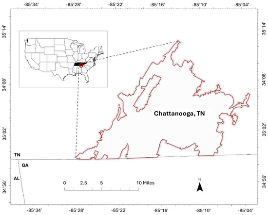
Figure 1.
Map showing the location and extent of the study site. The red circle indicates the location of the study site in the state of Tennessee.
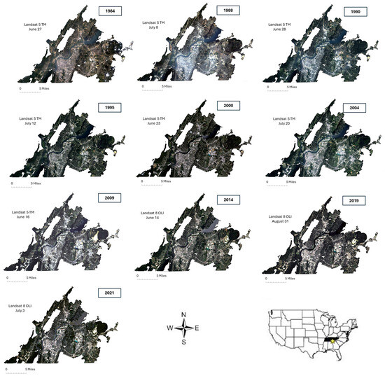
Figure 2.
The time series of Landsat 5 TM and Landsat 8 OLI images used for this study. Images are displayed in true color. The yellow star indicates the location of the study site.

Table 1.
Landsat 5 TM and Landsat 8 OLI sensor specifications.
In order to understand how forest canopy coverage was impacted by urbanization between 1984 and 2021, imagery was obtained along a defined interval, where the years between imagery acquisition (referred to in Table 2 as ‘Acquisition Gap’) was equal to or less than 5 years. A 5-year interval was selected by the researchers to effectively observe urban growth and canopy loss through time without obtaining an excessive number of Landsat scenes. In this research a total of 10 scenes were obtained representing 37 years of urbanization in the City of Chattanooga, TN. All Landsat scenes were obtained during the months of June and July to account for any seasonal variation in canopy coverage except the one acquired in 2019.
Table 2.
List of the acquired Landsat 5 TM and Landsat 8 OLI imagery.
In some cases when cloud coverage was an issue, imagery was acquired before the defined 5-year interval. In one case, however, the acquisition period between scenes was greater than the defined 5-year interval. This was due to excessive cloud coverage above Chattanooga, TN between the months of June and July from 2014 to 2020. For this reason, the acquisition gap between scenes 8 and 9 was 6 years instead of 5 years.
The flowchart in Figure 3 summarizes the workflows adopted in the methodology of this study.
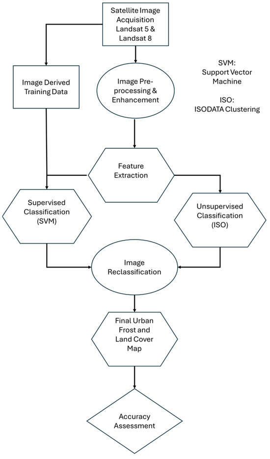
Figure 3.
A flowchart summarizes the workflows adopted in the methodology of this study.
2.2. Data Processing
The acquired image time series was processed using digital image processing (DIP) techniques [46]. The processing was performed using the DIP tools available on ERDAS Imagine 2020 and ArcGIS Pro 3.1 software. The images were acquired and processed as part of a master’s thesis research conducted by William Stuart [47]. The specific image processing steps performed are explained below.
2.2.1. Image Pre-Processing and Enhancement
Using ERDAS Imagine’s layer stack tool, the individual bands for each of the downloaded scenes, as shown in Table 1 and Table 2, were stacked to create 10 composite multispectral images. Next, using ArcGIS Pro’s raster geoprocessing tool, each of the 10 composite images were clipped to the City of Chattanooga’s boundary (Figure 1). From each of the 10 scenes, a true color image was derived using ArcGIS Pro. For Landsat 5 scenes 1–7, the band combination for RGB true color was 321. For Landsat 8 scenes 8–10, the band combination for RGB was 432. The images were then stretched using either percent clip or standard deviation depending on the clarity of the image after applying a stretch. Figure 2 shows the time series of Landsat 5 TM and Landsat 8 OLI images (from 1984 to 2021) used for this study. The images are shown in true color.
2.2.2. Feature Extraction
The next step in digital image processing was classifying each image to obtain a thematic land cover map in the following classes: developed areas, forest canopy, non-forest vegetation, and water. To accomplish this, both pixel-based supervised classification and pixel-based unsupervised classification were utilized. This is commonly referred to as a supervised hybrid classification strategy. For reasons related to Landsat’s 30 m spatial resolution, pixel-based supervised hybrid classification was ultimately selected.
2.2.3. Supervised Classification
The image classification wizard available on ArcGIS Pro was used to conduct supervised classification [46,47,48]. The classification was realized using the pixel-based approach relying on the training samples derived from the image. Figure 4 shows examples of the training sample polygons shown on the Landsat 8 OLI image acquired in 2021. The pixels of the images were classified into three classes: pervious surfaces, impervious surfaces, and water. The support vector machine algorithm was used as the machine learning classifier for supervised classification.
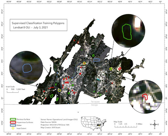
Figure 4.
Distribution of training samples used for supervised classification shown on the true color 2021 Landsat 8 OLI imagery.
Satellite imagery acquired through the Landsat program has been widely used for land use and land cover mapping since 1972 [49,50]. The supervised classification technique using the Maximum Likelihood Classification (MLC) algorithm is the most popular and conventional method to perform a land use and land cover classification task with an acceptable rate of accuracy. The MLC classification is based on a parametric approach which implies the assumption of the selected signature classes within the normal distribution [51], which is not certain about the current study. Recent studies show that some non-parametric based classification techniques have been used for extracting major classification as well as sub-classification with better accuracy [52]. The widely used non-parametric classification techniques are Decision Trees, Fuzzy C-Mean, Artificial Neural Networks (ANN), and Support Vector Machines (SVMs). Among them, SVMs have been reported to classify satellite imagery to generate land use and land cover maps with better accuracy in comparison to MLC classification [53,54]. That is why this research used an SVM as the algorithm for supervised classification.
An SVM is based on statistical theory and is used for classification and regression problems [55,56]. It is defined as a machine learning algorithm that uses supervised learning models to solve complex classification tasks by performing optimal data transformations that determine boundaries between data points based on predefined classes. The primary objective behind SVMs is to transform the input data into a higher-dimensional feature space (hyperplane). This transformation makes it easier to find a linear separation between classes in the imagery. It is considered one of the best supervised classification algorithms because of its capability to handle high-dimensional data. It is very effective in cases with limited training samples.
The output data obtained from supervised classification were 10 raster datasets each consisting of 3 land cover classes: pervious surfaces, impervious surfaces, and water. Figure 5 shows the result of the supervised classification obtained for the 2021 image.
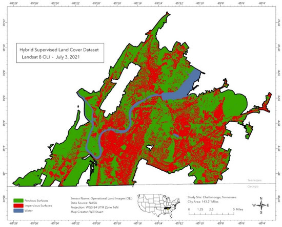
Figure 5.
Three class thematic land cover dataset derived from the supervised classification of the 2021 Landsat 8 OLI imagery.
2.2.4. Unsupervised Classification
Using ArcGIS Pro’s geoprocessing tool (Extract by Mask), pixels from the original multispectral Landsat images coincident with the pervious surface class from the output of the previous step were extracted. In this step, unsupervised pixel-based classification [46,47,48] within ArcGIS Pro’s image classification wizard was employed to classify the extracted multispectral pervious pixels into 10 spectrally unique classes. An ISODATA clustering [46,47,48] algorithm was used as the classifier for unsupervised classification. The maximum number of classes was set to 10. The output data obtained from unsupervised classification were 10 raster datasets, each consisting of 10 spectrally distinct classes of pervious pixels. Figure 6 shows the result of the unsupervised classification for the 2021 image.
2.2.5. Post Processing—Image Reclassification
The unsupervised classification outputs needed to be reclassified into 2-class rasters consisting of forest canopy or non-forest vegetation. This was accomplished using a true color reference to inspect each of the 10 classes of pervious pixels for all unsupervised outputs. After determining whether each class of the unsupervised outputs belonged to the forest canopy class or the non-forest vegetation class, the unsupervised output was reclassified using ArcGIS Pro’s geoprocessing tool (reclassify). The output obtained from the reclassification of unsupervised data was 10 raster datasets, each consisting of forest canopy and non-forest vegetation. Figure 7 shows the result obtained after reclassification for the 2021 image.

Figure 6.
Land cover output consisting of 10 spectrally distinct classes of pervious pixels (following unsupervised classification) for the 2021 Landsat 8 OLI imagery. Each color indicates a distinct feature within the extracted pervious surfaces.
Figure 6.
Land cover output consisting of 10 spectrally distinct classes of pervious pixels (following unsupervised classification) for the 2021 Landsat 8 OLI imagery. Each color indicates a distinct feature within the extracted pervious surfaces.


Figure 7.
Reclassification of 10 spectrally distinct classes of previous pixels to a 2-class thematic raster consisting of non-forest vegetation and forest vegetation derived from 2021 Landsat 8 OLI imagery.
Figure 7.
Reclassification of 10 spectrally distinct classes of previous pixels to a 2-class thematic raster consisting of non-forest vegetation and forest vegetation derived from 2021 Landsat 8 OLI imagery.

2.3. Data Analysis
Finally, to obtain the desired 4 class land cover map, the outputs from the reclassification of pervious pixels and supervised classification needed to be combined. From each of the supervised classification outputs, all pervious pixels were reclassified to ‘no data’ using ArcGIS Pro’s geoprocessing tool (reclassify). Next, using ArcGIS Pro’s raster function (merge), the developed and water classes from supervised classification and the forest and non-forest vegetation classes from unsupervised classification were combined. The final output data obtained were 10 raster datasets, each consisting of 4 classes: impervious surfaces, urban forest canopy, non-forest vegetation, and water (Table 3). Figure 8, Figure 9, Figure 10, Figure 11, Figure 12, Figure 13, Figure 14, Figure 15, Figure 16 and Figure 17 show the final output for all 10 images.
Table 3.
Final thematic land cover dataset class names and descriptions.
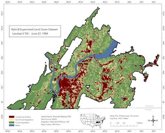
Figure 8.
Final supervised hybrid thematic 4-class land cover raster of 1984.
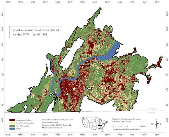
Figure 9.
Final supervised hybrid thematic 4-class land cover raster of 1988.
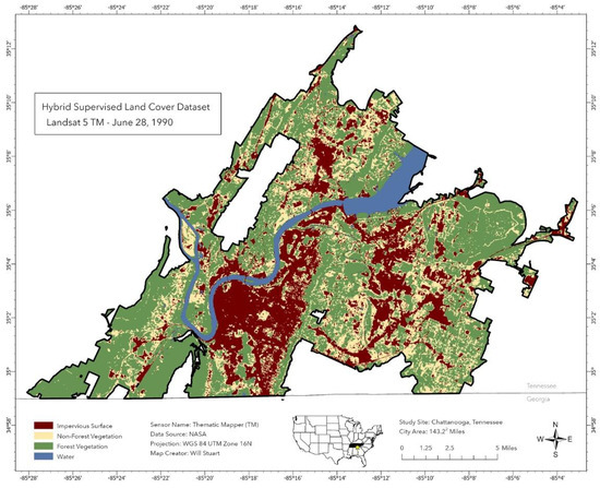
Figure 10.
Final supervised hybrid thematic 4-class land cover raster of 1990.
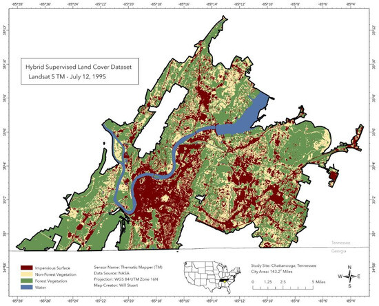
Figure 11.
Final supervised hybrid thematic 4-class land cover raster of 1995.
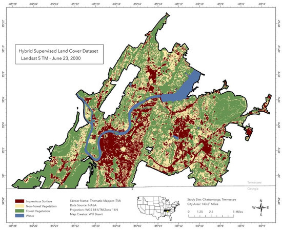
Figure 12.
Final supervised hybrid thematic 4-class land cover raster of 2000.
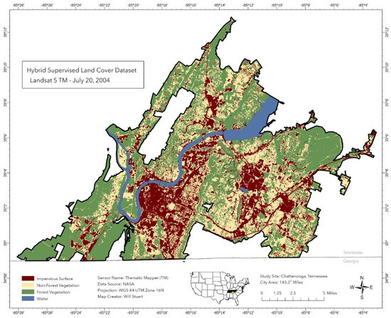
Figure 13.
Final supervised hybrid thematic 4-class land cover raster of 2004.
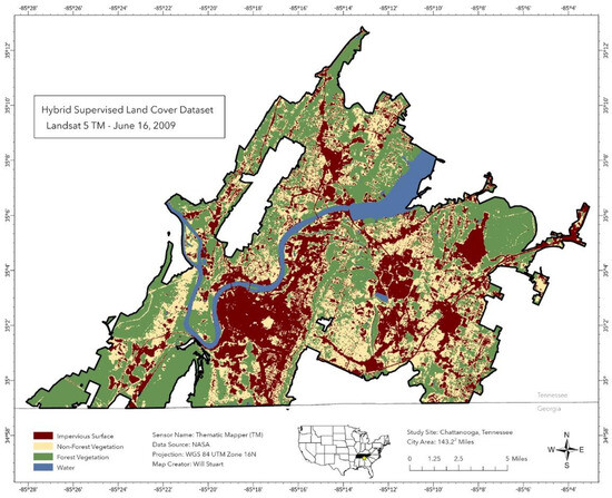
Figure 14.
Final supervised hybrid thematic 4-class land cover raster of 2009.
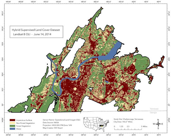
Figure 15.
Final supervised hybrid thematic 4-class land cover raster of 2014.
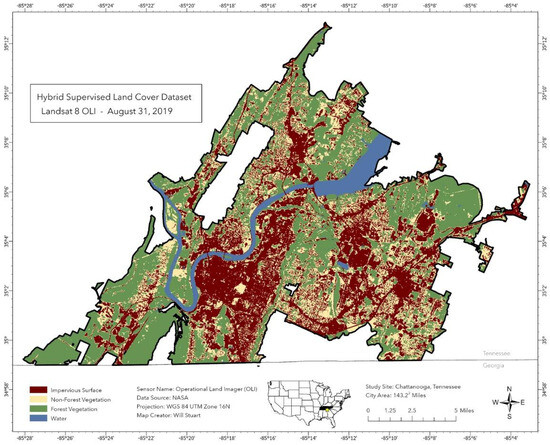
Figure 16.
Final supervised hybrid thematic 4-class land cover raster of 2019.
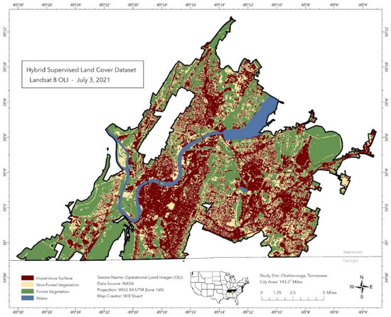
Figure 17.
Final supervised hybrid thematic 4-class land cover raster of 2021.
2.4. Accuracy Assessment
Typically, accuracy assessments of spatial analyses incorporate ground-truth data to reference the derived land cover dataset. However, this is not possible when dealing with temporal datasets. Therefore, Google Earth’s historic imagery archive was utilized as a proxy for ground-truth reference data. For each year of acquisition for the Landsat imagery obtained in this research, polygons representing pure samples of the 4 classes (Table 3) derived in the final output of this analysis were collected using random stratified sampling across Google Earth’s historic imagery and saved as separate KML files (Figure 18). The files were then uploaded to ArcGIS Pro and saved as feature classes. Finally, using ArcGIS Pro’s geoprocessing tool, confusion matrices were prepared, and an analysis of producer accuracy, user accuracy, and overall accuracy [57,58,59] was performed for each year. The user’s accuracy is calculated by dividing the total number of classified pixels that match the reference pixels by the total number of classified pixels for that class. The producer’s accuracy is calculated by dividing the total number of classified pixels that match the reference pixels by the total number of reference pixels for that class. Overall accuracy is the probability that an individual feature will be correctly classified with a classification algorithm. It is calculated by dividing the sum of the match pixels of all classes (with corresponding reference pixels) by the total number of pixels classified [57,58,59].
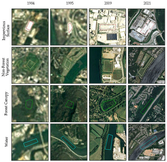
Figure 18.
Examples of the reference polygons that were used to conduct the accuracy assessment of the land cover datasets produced in this study. These polygons were digitized using Google Earth’s historic imagery. Here, polygons that were digitized for 1984, 1995, 2009, and 2021 Landsat imagery are shown. The color frames indicate reference polygons for different features. Images not to scale.
3. Results and Analysis
3.1. Quantification of Land Cover Classes
Areas and relative percentages of land cover classes were quantified for the 10 final land cover datasets. The results are shown in Table 4.
Table 4.
Quantification of land cover classes. Non-Forest Vegetation is symbolized by NF.
3.2. Assessment of Spatiotemporal Trends
Figure 19 displays the area of each land cover class in acres for all ten images in a bar chart. The area in acres and the relative percentage of each land cover class for all images is also provided in Table 4. Finally, the percent change in land cover classes between consecutive imagery dates was calculated and provided in Table 5. As indicated by the final land cover class area estimations, since 1984, Chattanooga has steadily lost forest canopy. In the last 37 years between 1984 and 2021, this study estimates that Chattanooga has lost approximately 36.9 sq mi of its urban forest canopy. These losses in forest canopy are replaced by steady gains in impervious surface areas. Since 1984 Chattanooga’s urban spaces have gained 32.5 sq mi, an increase of approximately 134%.
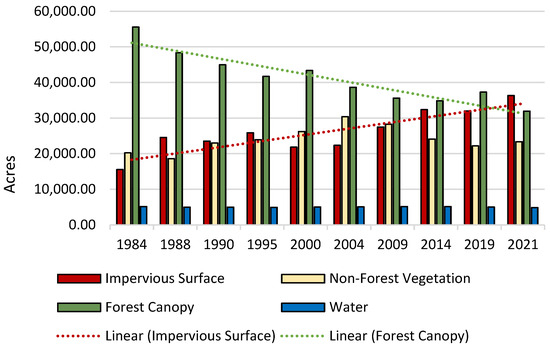
Figure 19.
Land cover class area in acres for the 10 final land cover datasets.
Table 5.
Land cover class area percent change between imagery acquisition dates.
The most significant change in impervious surface areas between consecutive images occurred between 1984 and 1988. During this time, Chattanooga’s urban spaces increased in area by approximately 58%, while urban forest area decreased by 13%. The most significant change in urban forest canopy surface area occurred between 2019 and 2021. During this period, urban forest areas decreased by 14%, while impervious surface area increased by 14%. In two separate instances, the percent change in urban forest canopy is positive rather than negative, suggesting a net growth in urban forest canopy. The first instance, occurring between 1995 and 2000, is complemented by an increase of approximately 10% of non-forest vegetation.
In recent years, the City of Chattanooga has undergone steady population growth, mostly due to rapid economic growth [60], which is heavily favored by its geographic location. The city is home to several large organizations such as Volkswagen, Unum, Tennessee Valley Authority, Blue Cross Blue Shield, Wacker, and Amazon that are driving the area’s economic growth. The economic growth of the city is strongly attributed to the implementation of the fiber optic internet by the City’s Electric Power Board (EPB). With numerous large corporations continuing to expand, a nationally ranked internet infrastructure, and a supported nickname as the “Scenic City”, Chattanooga’s economic and social environment is becoming increasingly attractive to startup businesses. The city has also designated a large part of the downtown area for startups, small businesses, nonprofits, and government offices called the “Innovation District” [61]. These clearly indicate the underlying reasons for the continuous growth of urban areas in Chattanooga, and thereby support the trends of changes in urban forest canopy revealed in this study.
3.3. Accuracy Assessment
For each of the classified land cover datasets, a confusion matrix was generated (Table 6 and Table 7). Based on the results of the accuracy assessments conducted for the ten land cover datasets, overall accuracy ranged from 92.97% to 99.71%. Scene 10 (2021) yielded the highest overall accuracy, while Scene 1 (1984) produced the lowest. Results across all ten accuracy assessments suggest the most common error of commission (Type I error/false-positive) was the erroneous classification of non-forest vegetation pixels into the impervious surface and forest canopy land classes. The most common error of omission (Type II error/false-negative) was the erroneous classification of impervious surface pixels into the non-forest vegetation and forest canopy land classes. Based on the results from the accuracy assessments, the methodology utilized in this research is capable of classifying forest canopy pixels apart from other land cover classes using moderate resolution Landsat 5 TM imagery and Landsat 8 OLI imagery at the city-scale with substantial accuracy.
Table 6.
Confusion matrices derived from the accuracy assessment of 1984–2000 land cover datasets.
Table 7.
Confusion matrices derived from the accuracy assessment of 2004–2021 land cover datasets.
4. Discussion
The main objective of this research was to identify the extent of urban forest across the City of Chattanooga, TN. In conducting this research, Landsat 5 and 8 data were obtained. However, Landsat 5 and 8 are two different systems designed three decades apart. Therefore, image quality between these systems is inherently different. Additionally, variable levels of atmospheric dust, pollen, and water vapor can impact the accuracy of a remote sensor. For this reason, a supervised hybrid classification workflow as described in this research was implemented in lieu of more traditional classification methods to normalize potential variation across classified results. In addition, the use of Level-2 calibrated surface reflectance images should minimize the uncertainty between the two sensor systems. However, it is recommended to apply more advanced machine learning techniques such as Artificial Neural Network (ANN) and/or Deep Learning (DL) models to expand this research further in the future.
To accurately classify the extent of forest canopy in each of the images, it is necessary to delineate tree pixels from pixels representing non-tree types of vegetation. However, because of Landsat’s moderate 30 m spatial resolution, and the spectral similarities between tree pixels and non-tree pixels, it is highly difficult to visually differentiate between forest canopy and non-forest vegetation, even when viewing the imagery in false color. This was especially true in residential areas. Similarly, many developed residential areas in Chattanooga have higher quantities of forest canopy compared to developed non-residential areas in the city. However, the forest canopy in these residential areas is unlike a natural forested area. In residential areas, the forest canopy is highly fragmented and mixed in thoroughly with other non-forest vegetation and impervious surfaces. As a result, it becomes hard to draw the line between forest canopy, non-forest vegetation, and developed land areas within residential areas throughout Chattanooga. In other words, due to Landsat’s limited 30 m spatial resolution and the spectral similarities between tree pixels and non-tree vegetation pixels, it is difficult to visually differentiate between forest and non-forest vegetation, especially in residential areas, where fragments of forest, non-forest vegetation, and developed land classes are packed together in an area smaller than Landsat’s spatial resolution. Therefore, this research opted to utilize unsupervised classification for pervious pixel classification, as there was a greater chance for the computer to spectrally differentiate between forest and non-forest vegetation pixels. The suggested use of ANN and/or DL algorithms potentially should resolve this issue further.
Ultimately, the issues as described here can be tied back to the spatial resolution of Landsat, but also to the scale of the objects being classified. Because many of the non-forest vegetation pixels represent vegetation that has been re-planted by people physically within developed areas, and these re-planted areas of non-forest vegetation are typically smaller than 30 m, such as, for example, a flower garden or a grassy lawn, it is possible for non-forest vegetation pixels to blend with the adjacent developed and forest canopy pixels due to the moderate spatial resolution of Landsat. The pan-sharpening technique can be useful in this regard for Landsat 7 and Landsat 8. However, since Landsat 5 does not have a panchromatic band, this approach cannot be used for the entire time series.
Object-based supervised classification is a relatively new concept that groups spectrally similar and spatially clustered pixels into objects or segments, then conducts classification on the segments. One caveat to object-based classification is that it is typically utilized with fine spatial resolution sensors. Additionally, segmentation is a computationally demanding process that requires a distributed processing environment. However, it is strongly recommended to apply object-based supervised classification to expand this research further to see if this approach could generate better results.
Cloud coverage is always a challenge for any optical sensors. Although this research only used Landsat imagery, future research should consider using imagery from other similar optical sensors at least for the recent dates of the time series to minimize the possibility of large data gaps.
To future researchers conducting spatial analyses, when building temporal datasets for spatiotemporal analyses, it is often common to attempt to acquire as much data as possible within a defined acquisition period. However, when working with many multispectral datasets, generating classified outputs that are similar enough to each other that, when viewed chronologically, the under classification or over classification of a given class is not directly obvious is quite difficult. Therefore, it could be helpful to only acquire data around the beginning and end of the defined temporal scope of a research project, as the net loss/gained, and percent change is commonly the information desired by the researcher and other stakeholders.
The main objective of this research was to detect, map, and quantify the historical coverage of the urban forest in Chattanooga, TN. To reduce confusion, this research did not expand the analysis further. However, it is recommended to add more analysis to expand this research further in the future. In addition, it would also be useful to include analysis of how different types of land use and land cover during the urbanization process specifically affect the forest ecosystem.
5. Conclusions
This research was designed to detect and map the historic extent of Chattanooga’s urban forest canopy from 1984 to 2021 using remote sensing technology. This research took advantage of the extensive temporal archive of multispectral satellite imagery provided by the Landsat program to conduct a 37-year land cover change analysis across Chattanooga, Tennessee.
This study shows that since 1984 the forest canopy in Chattanooga regularly decreased. During the 37-year time span between 1984 and 2021, Chattanooga lost approximately 36.9 sq mi of its urban forest canopy. These losses in the forest canopy were replaced by steady gains in impervious surface areas. Since 1984, Chattanooga’s urban spaces have gained 32.5 sq mi, an increase of approximately 134%.
Based on the obtained results, it can be concluded that, despite the limitations in spatial resolution, Landsat satellite images can be effectively used for mapping and analyzing the multidecade spatiotemporal forest canopy in a rapidly expanding metropolitan center, such as Chattanooga, TN. The data generated in this research and the developed image processing method have great potential to help direct sustainable development efforts towards areas urbanizing at an above-average rate.
Author Contributions
Conceptualization, W.S. and A.H.; methodology, W.S. and A.H.; software, W.S., A.H. and N.H.; validation, W.S. and A.H.; formal analysis, W.S.; investigation, W.S. and A.H.; resources, W.S., A.H., C.M. and N.H.; data curation, W.S. and A.H.; writing—original draft preparation, W.S. and A.H.; writing—review and editing, W.S., A.H., C.M., N.H. and H.Q.; visualization, W.S. and A.H.; supervision, A.H.; project administration, A.H. All authors have read and agreed to the published version of the manuscript.
Funding
This research received no external funding.
Data Availability Statement
The raw data supporting the conclusions of this article will be made available by the authors on request.
Acknowledgments
Thanks are due to NASA/USGS for providing the Landsat satellite images at no cost. Thanks are also due to the University of Tennessee at Chattanooga for providing access to the necessary geospatial software such as ArcGIS Pro and Erdas Imagine conducting the research.
Conflicts of Interest
The authors declare no conflicts of interest.
References
- Reich, P.B.; Bolstad, P. Productivity of Evergreen and Deciduous Temperate Forests. Terrestrial Global Productivity; Academic Press: San Diego, CA, USA, 2001; pp. 245–283. [Google Scholar]
- Malhi, Y.A.; Baldocchi, D.; Jarvis, P. The carbon balance of tropical, temperate, and boreal forests. Plant Cell Environ. 1999, 22, 715–740. [Google Scholar] [CrossRef]
- Bundestag, D. Protecting the Tropical Forests: A High Priority Task; Woods-Schank, G., Translator; Deutscher Bundestag, Referat Öffentlichkeitsarbet: Bonn, Germany, 1990; p. 968. [Google Scholar]
- Heath, L.S.; Kauppi, P.E.; Burschel, P.; Gregor, H.D.; Guderian, R.; Kohlmaier, G.H.; Thomasius, H. Contribution of temperate forests to the world’s carbon budget. Water Air Soil Pollut. 1993, 70, 55–69. [Google Scholar] [CrossRef]
- Pan, Y.; Birdsey, R.A.; Phillips, O.L.; Jackson, R.B. The Structure, Distribution, and Biomass of the World’s Forests. Annu. Rev. Ecol. Evol. Syst. 2013, 44, 593–622. [Google Scholar] [CrossRef]
- FAO. Global Forest Resources Assessment 2020—Key Findings; Food and Agriculture Organization of the United Nations: Rome, Italy, 2020; p. 186. [Google Scholar]
- Kindermann, G.; Obersteiner, M.; Sohngen, B.; Sathaye, J.; Andrasko, K.; Rametsteiner, E.; Beach, R. Global cost estimates of reducing carbon emissions through avoided deforestation. Proc. Natl. Acad. Sci. USA 2008, 105, 10302–10307. [Google Scholar] [CrossRef]
- Lorenz, K.; Lal, R. Carbon Sequestration in Forest Ecosystems; Springer: Dordrecht, The Netherlands; Berlin/Heidelberg, Germany; London, UK; New York, NY, USA, 2009; p. 279. [Google Scholar]
- IPCC. Climate Change and Land: IPCC Special Report on Climate Change, Desertification, Land Degradation, Sustainable Land Management, Food Security, and Greenhouse Gas Fluxes in Terrestrial Ecosystems; Cambridge University Press: Cambridge, UK, 2022; pp. 1–36. [Google Scholar]
- Brandão, M.; Levasseur, A.; Kirschbaum, M.U.; Weidema, B.P.; Cowie, A.L.; Jørgensen, S.V. Key issues and options in accounting for carbon sequestration and temporary storage in life cycle assessment and carbon footprinting. Int. J. Life Cycle Assess. 2013, 18, 230–240. [Google Scholar] [CrossRef]
- Tans, P.P.; Fung, I.Y.; Akahashi, T. Observational constraints on the global atmospheric CO2 budget. Science 1990, 247, 1431–1438. [Google Scholar] [CrossRef]
- Schimel, D.S. Terrestrial ecosystems and the carbon cycle. Glob. Chang. Biol. 1995, 1, 77–91. [Google Scholar] [CrossRef]
- Spicer, M.E.; Mellor, H.; Carson, W.P. Seeing beyond the trees: A comparison of tropical and temperate plant growth forms and their vertical distribution. Ecology 2020, 101, e02974. [Google Scholar] [CrossRef]
- Seto, K.C.; Sánchez-Rodríguez, R.; Fragkias, M. The new geography of contemporary urbanization and the environment. Annu. Rev. Environ. Resour. 2010, 35, 167–194. [Google Scholar] [CrossRef]
- Hossain, A.; Stuart, W.; Mies, J.; Brock-Hon, A. Investigating Urban Heat Island (UHI) Impact for the City of Chattanooga, Tennessee Using GIS and Remote Sensing. In Handbook of Climate Change Mitigation and Adaptation; Lackner, M., Sajjadi, B., Chen, W.Y., Eds.; Springer: New York, NY, USA, 2021; pp. 1–35. [Google Scholar]
- Nowak, D.J.; Noble, M.H.; Sisinni, S.M.; Dwyer, J.F. People and trees: Assessing the US urban forest resource. J. For. 2001, 99, 37–42. [Google Scholar] [CrossRef]
- Nowak, D.J.; Hoehn, R.E.; Bodine, A.R.; Greenfield, E.J.; O’Neil-Dunne, J. Urban forest structure, ecosystem services and change in Syracuse, NY. Urban Ecosyst. 2016, 19, 1455–1477. [Google Scholar] [CrossRef]
- Endreny, T.A. Strategically growing the urban forest will improve our world. Nat. Commun. 2018, 9, 1–3. [Google Scholar] [CrossRef]
- Nowak, D.J.; Greenfield, E.J. US urban forest statistics, values, and projections. J. For. 2018, 116, 164–177. [Google Scholar] [CrossRef]
- Fornal-Pieniak, B.; Ollik, M.; Schwerk, A. Impact of different levels of anthropogenic pressure on the plant species composition in woodland sites. Urban For. Urban Green. 2019, 38, 295–304. [Google Scholar] [CrossRef]
- Aryal, P.C.; Aryal, C.; Bhusal, K.; Chapagain, D.; Dhamala, M.K.; Maharjan, S.R. Forest structure and anthropogenic disturbances regulate plant invasion in urban forests. Urban Ecosyst. 2022, 25, 367–377. [Google Scholar] [CrossRef]
- Nowak, D.J.; Dwyer, J.F. Understanding the Benefits and Costs of Urban Forest Ecosystems. In Urban and Community Forestry in the Northeast; Kuser, J.E., Ed.; Springer: Dordrecht, The Netherlands, 2007; pp. 25–46. [Google Scholar]
- Davis, K.L. The Role of Sense of Place: A Theoretical Framework to Aid Urban Forest Decision-Making. Ph.D. Thesis, The University of Tennessee, Knoxville, TN, USA, 2011. [Google Scholar]
- Livesley, S.; McPherson, E.G.; Calfapietra, C. The urban forest and ecosystem services: Impacts on urban water, heat, and pollution cycles at the tree, street, and city scale. J. Environ. Qual. 2016, 45, 119–124. [Google Scholar] [CrossRef]
- Albiero-Júnior, A.; Venegas-González, A.; Rodríguez-Catón, M.; Oliveira, J.M.; Longhi-Santos, T.; Galvão, F.; Botosso, P.C. Edge effects modify the growth dynamics and climate sensitivity of Araucaria angustifolia trees. Tree-Ring Res. 2020, 76, 11–26. [Google Scholar] [CrossRef]
- Morreale, L.L.; Thompson, J.R.; Tang, X.; Reinmann, A.B.; Hutyra, L.R. Elevated growth and biomass along temperate forest edges. Nat. Commun. 2021, 12, 1–8. [Google Scholar]
- Garvey, S.M.; Templer, P.H.; Pierce, E.A.; Reinmann, A.B.; Hutyra, L.R. Diverging patterns at the forest edge: Soil respiration dynamics of fragmented forests in urban and rural areas. Glob. Chang. Biol. 2022, 28, 3094–3109. [Google Scholar] [CrossRef]
- Muukkonen, P.; Heiskanen, J. Biomass estimation over a large area based on standwise forest inventory data and ASTER and MODIS satellite data: A possibility to verify carbon inventories. Remote Sens. Environ. 2007, 107, 617–624. [Google Scholar] [CrossRef]
- Li, B.; Xu, X.; Zhang, L.; Han, J.; Bian, C.; Li, G.; Jin, L. Above-ground biomass estimation and yield prediction in potato by using UAV-based RGB and hyperspectral imaging. ISPRS J. Photogramm. Remote Sens. 2020, 162, 161–172. [Google Scholar] [CrossRef]
- Alrababah, M.A.; Alhamad, M.N.; Bataineh, A.L.; Bataineh, M.M.; Suwaileh, A.F. Estimating east Mediterranean forest parameters using Landsat ETM. Int. J. Remote Sens. 2011, 32, 1561–1574. [Google Scholar] [CrossRef]
- Castillo, J.A.A.; Apan, A.A.; Maraseni, T.N.; Salmo III, S.G. Estimation and mapping of above-ground biomass of mangrove forests and their replacement land uses in the Philippines using Sentinel imagery. ISPRS J. Photogramm. Remote Sens. 2017, 134, 70–85. [Google Scholar] [CrossRef]
- Duncan, J.M.A.; Boruff, B.; Saunders, A.; Sun, Q.; Hurley, J.; Amati, M. Turning down the heat: An enhanced understanding of the relationship between urban vegetation and surface temperature at the city scale. Sci. Total Environ. 2019, 656, 118–128. [Google Scholar] [CrossRef]
- Zhang, L.; Shao, Z.; Liu, J.; Cheng, Q. Deep learning based retrieval of forest aboveground biomass from combined LiDAR and Landsat 8 data. Remote Sens. 2019, 11, 1459. [Google Scholar] [CrossRef]
- Jensen, J.R. Remote Sensing of the Environment: An Earth Resource Perspective; Pearson Prentice Hall: Hoboken, NJ, USA, 2007; p. 544. [Google Scholar]
- Bourgoin, C.; Blanc, L.; Bailly, J.S.; Cornu, G.; Berenguer, E.; Oszwald, J.; Gond, V. The potential of multisource remote sensing for mapping the biomass of a degraded Amazonian forest. Forests 2018, 9, 303. [Google Scholar] [CrossRef]
- Foody, G.M.; Boyd, D.S.; Cutler, M.E. Predictive relations of tropical forest biomass from Landsat TM data and their transferability between regions. Remote Sens. Environ. 2003, 85, 463–474. [Google Scholar] [CrossRef]
- Cohen, W.B.; Maiersperger, T.K.; Gower, S.T.; Turner, D.P. An improved strategy for regression of biophysical variables and Landsat ETM+ data. Remote Sens. Environ. 2003, 84, 561–571. [Google Scholar] [CrossRef]
- Frazier, R.J.; Coops, N.C.; Wulder, M.A.; Kennedy, R. Characterization of aboveground biomass in an unmanaged boreal forest using Landsat temporal segmentation metrics. ISPRS J. Photogramm. Remote Sens. 2014, 92, 137–146. [Google Scholar] [CrossRef]
- Gómez, C.; White, J.C.; Wulder, M.A.; Alejandro, P. Historical forest biomass dynamics modelled with Landsat spectral trajectories. ISPRS J. Photogramm. Remote Sens. 2014, 93, 14–28. [Google Scholar] [CrossRef]
- Tian, X.; Li, Z.; Su, Z.; Chen, E.; van der Tol, C.; Li, X.; Ling, F. Estimating montane forest above-ground biomass in the upper reaches of the Heihe River Basin using Landsat-TM data. Int. J. Remote Sens. 2014, 35, 7339–7362. [Google Scholar] [CrossRef]
- Gu, C.; Clevers, J.G.; Liu, X.; Tian, X.; Li, Z.; Li, Z. Predicting forest height using the GOST, Landsat 7 ETM+, and airborne LiDAR for sloping terrains in the Greater Khingan Mountains of China. ISPRS J. Photogramm. Remote Sens. 2018, 137, 97–111. [Google Scholar] [CrossRef]
- Izadi, S.; Sohrabi, H.; Khaledi, M.J. Estimation of coppice forest characteristics using spatial and non-spatial models and Landsat data. J. Spat. Sci. 2020, 67, 143–156. [Google Scholar] [CrossRef]
- Jenner, L. Landsat Overview. Available online: https://www.nasa.gov/mission_pages/landsat/overview/index.html (accessed on 27 October 2020).
- Blanton, R.; Hossain, A. Mapping the Recovery Process of Vegetation Growth in the Copper Basin, Tennessee Using Remote Sensing Technology. GeoHazards 2020, 1, 31–43. [Google Scholar] [CrossRef]
- Hall, J.; Hossain, A. Mapping urbanization and evaluating its possible impacts on stream water quality in Chattanooga, Tennessee, using GIS and remote sensing. Sustainability 2020, 12, 1980. [Google Scholar] [CrossRef]
- Jensen, J.R. Introductory Digital Image Processing: A Remote Sensing Perspective; Prentice-Hall: Upper Saddle River, NJ, USA, 2015; pp. 1–544. [Google Scholar]
- Stuart, W. Mapping Urban Forest Extent and Modeling Sequestered Carbon Across Chattanooga, Tennessee’s Urban Forest Canopy Using GIS and Remote Sensing Principles. Unpublished Thesis, The University of Tennessee at Chattanooga, Chattanooga, TN, USA, 2023. [Google Scholar]
- Lillesand, T.M.; Kiefer, R.W. Remote Sensing and Image Interpretation; John Willey and Sons, Inc.: Hoboken, NJ, USA, 2000; pp. 1–724. [Google Scholar]
- Townshend, J.R.G. Land cover. Int. J. Remote Sens. 1992, 13, 1319–1328. [Google Scholar] [CrossRef]
- Lu, D.; Weng, Q. A survey of image classification methods and techniques for improving classification performance. Int. J. Remote Sens. 2007, 28, 823–870. [Google Scholar] [CrossRef]
- Srivastava, P.K.; Kiran, G.; Gupta, M.; Sharma, N.; Prasad, K. A study on distribution of heavy metal contamination in vegetables using GIS and analytical technique. Int. J. Ecol. Dev. 2012, 21, 89–99. [Google Scholar]
- Kavzoglu, T.; Reis, S. Performance analysis of maximum likelihood and artificial neural network classifiers for training sets with mixed pixels. GIScience Remote Sens. 2008, 45, 330–342. [Google Scholar] [CrossRef]
- Szuster, B.W.; Chen, Q.; Borger, M. A comparison of classification techniques to support land cover and landuse analysis in tropical coastal zones. Appl. Geogr. 2011, 31, 525–532. [Google Scholar] [CrossRef]
- Yu, L.; Porwal, A.; Holden, E.J.; Dentith, M.C. Towards automatic lithological classification from remote sensing data using support vector machines. Comput. Geosci. 2021, 45, 229–239. [Google Scholar] [CrossRef]
- Vapnik, V.N. The Nature of Statistical Learning Theory; Springer: New York, NY, USA, 1995; pp. 1–334. [Google Scholar]
- Kavzoglu, T.; Colkesen, I. A kernel functions analysis for support vector machines for land cover classification. Int. J. Appl. Earth Obs. Geoinf. 2009, 11, 352–359. [Google Scholar] [CrossRef]
- Fitzgerald, R.; Lees, B. Assessing the classification accuracy of multisource remote sensing data. Remote Sens. Environ. 1994, 47, 362–368. [Google Scholar] [CrossRef]
- Masson, L.F.; MCNeill, G.; Tomany, J.; Simpson, J.; Peace, H.S.; Wei, L.; Grubb, D.; Bolton-Smith, C. Statistical approaches for assessing the relative validity of a food-frequency questionnaire: Use of correlation coefficients and the kappa statistic. Public Health Nutr. 2003, 6, 313–321. [Google Scholar] [CrossRef]
- Reed, J.A.; Ainsworth, B.E.; Wilson, D.K.; Mixon, G.; Cook, A. Awareness and use of community walking trails. Prev. Med. 2004, 39, 903–908. [Google Scholar] [CrossRef]
- Cofer, B. Gross to Green: City Makes Strides to Becoming Sustainable; The Times Free Press: Chattanooga, TN, USA, 2011. [Google Scholar]
- Sohn, P. Chattanooga Creek Still Threatened; The Times Free Press: Chattanooga, TN, USA, 2010. [Google Scholar]


Disclaimer/Publisher’s Note: The statements, opinions and data contained in all publications are solely those of the individual author(s) and contributor(s) and not of MDPI and/or the editor(s). MDPI and/or the editor(s) disclaim responsibility for any injury to people or property resulting from any ideas, methods, instructions or products referred to in the content. |
© 2024 by the authors. Licensee MDPI, Basel, Switzerland. This article is an open access article distributed under the terms and conditions of the Creative Commons Attribution (CC BY) license (https://creativecommons.org/licenses/by/4.0/).