Abstract
This study aims to establish a deep learning-based classification framework to efficiently and rapidly distinguish between coniferous and broadleaf forests across the Loess Plateau. By integrating the deep residual neural network (ResNet) architecture with transfer learning techniques and multispectral data from unmanned aerial vehicles (UAVs) and Landsat remote sensing data, the effectiveness of the framework was validated through well-designed experiments. The study began by selecting optimal spectral band combinations, using the random forest algorithm. Pre-trained models were then constructed, and model performance was optimized with different training strategies, considering factors such as image size, sample quantity, and model depth. The results indicated substantial improvements in the model’s classification accuracy and efficiency for reasonable image dimensions and sample sizes, especially for an image size of 3 × 3 pixels and 2000 samples. In addition, the application of transfer learning and model fine-tuning strategies greatly enhanced the adaptability and universality of the model in different classification scenarios. The fine-tuned model achieved remarkable performance improvements in forest-type classification tasks, increasing classification accuracy from 85% to 93% in Zhengning, from 89% to 96% in Yongshou, and from 86% to 94% in Baishui, as well as exceeding 90% in all counties. These results not only confirm the effectiveness of the proposed framework, but also emphasize the roles of image size, sample quantity, and model depth in improving the generalization ability and classification accuracy of the model. In conclusion, this research has developed a technological framework for effective forest landscape recognition, using a combination of multispectral data from UAVs and Landsat satellites. This combination proved to be more effective in identifying forest types than was using Landsat data alone, demonstrating the enhanced capability and accuracy gained by integrating UAV technology. This research provides valuable scientific guidance and tools for policymakers and practitioners in forest management and sustainable development.
1. Introduction
Forest ecosystems, as one of the most important ecosystems on Earth, play a critical role in maintaining biodiversity, regulating climate, and conserving soil and water [1,2]. With growing demands for global environmental governance and ecosystem protection, the need for the accurate monitoring and management of forest ecosystems has become increasingly urgent [3,4]. Effective forest monitoring requires advanced methodologies capable of handling large, complex datasets and providing accurate classifications.
The Loess Plateau, one of China’s key ecologically vulnerable zones, has historically been faced with severe environmental challenges, including soil erosion, vegetation degradation, and desertification, due to its long-term irrational land use, water scarcity, and harsh terrain and climatic conditions [5,6]. To address these problems, the Chinese government has undertaken several ecological restoration initiatives since the 1990s, most notably, large-scale tree planting and afforestation efforts which have substantially expanded the artificial forest cover on the Loess Plateau. Among these, coniferous and broadleaf forests, mostly artificial, have become the primary forest types in the region. They play a crucial role in preventing wind and sand fixation effects, improving soil quality, and conserving biodiversity [7,8,9]. In the face of escalating climate change and human activities, rapid and accurate identification and monitoring of these forest types is crucial for ecological restoration and sustainable management on the Loess Plateau.
In recent years, the rapid growth of remote sensing data resources and the swift development of deep learning technologies have unleashed unprecedented potential in the field of environmental monitoring [10,11,12]. In image classification, deep learning improves its capabilities in handling large, complex datasets, feature extraction, and image recognition mainly through data fusion, multiscale feature learning, and transfer learning [13,14]. These methods effectively uncover and integrate the latent value from different remote sensing data sources. Among them, transfer learning stands out as a powerful framework that excels in handling large heterogeneous data and quickly adapting to new environments. It leverages pre-trained models on popular deep learning architectures to accelerate and improve learning efficiency for new tasks, even with limited labeled data [15,16,17].
Residual Neural Networks (ResNet) is one of the most widely used models within deep learning architectures, particularly adept at image classification tasks [18,19,20,21]. It has been extensively applied in areas such as medical image diagnosis, identification of agricultural crops and pests, and soil property estimation [22,23,24].
In forest monitoring and classification, emerging UAV data (hyperspectral cameras, RGB imagery, oblique photography, and LiDAR) have significantly improved classification accuracy and efficiency due to their high flexibility and resolution [25,26,27]. Many studies focus on using transfer learning strategies, training these models on large and diverse datasets (such as ImageNet) as a pre-training source, and then fine-tuning them on specific small sample datasets. However, specific image recognition datasets such as ImageNet contain many object categories that are unrelated to specific applications, such as forest classification. This mismatch in category distribution reduces the ability of the model to transfer from the source domain to the target domain, thereby affecting its performance. The current research has underutilized data directly related to the task for pre-training. Investigating how models can better identify specific forest types is critical. Factors such as model depth, image size, and sample quantity also significantly affect performance [28,29,30,31]. In practical applications, it is essential to consider these factors comprehensively to optimize the performance of the ResNet model. Furthermore, due to the cost limitations of UAV data, these studies are often limited to small-plot applications. In contrast, medium- to low-resolution remote sensing data (Landsat, Sentinel, and GF-1) have improved the accuracy and efficiency of forest classification using deep learning techniques, while enabling large-scale classification [32,33,34,35]. However, they still fall short of the high-precision classification achieved by UAVs. Therefore, effectively identifying and selecting valuable features from integrated multi-source data using deep learning technologies has broad application prospects in expanding the application scope and efficiency of image classification. Some studies have made initial attempts, such as [36], which effectively applied crop classification by integrating UAV and satellite images through data augmentation, transfer learning, and multimodal fusion techniques. Reference [37] proposed an object-oriented convolutional neural network classification method combining Sentinel-2, RapidEye, and LiDAR data, one which significantly improved classification accuracy in complex forest areas. Reference [38] developed a novel mangrove species classification framework using spectral, texture, and polarization information from three spatial image sources. However, there remains room for optimization in utilizing transfer learning techniques to explore the potential of emerging high-resolution multispectral UAV data for landscape-scale forest classification, while achieving data complementarity and cross-domain enhancements to improve classification accuracy and expand application scope.
In response to these challenges, this study selected three counties in the Loess Plateau region with similar forest types—Yongshou, Baishui, and Zhengning—as research sites. Among them, the forests in Yongshou County were selected as the primary research object, while Baishui County and Zhengning County served as supplementary research sites to validate the applicability and generalizability of the developed model. Adopting a transfer learning approach, the study uses the ResNet model in conjunction with multi-resource remote sensing data to establish an effective framework for identifying forest types. The effects of different combination strategies (sample quantity, model depth, and image size) on the model performance will be explored. The main objectives of this study are: (1) to develop an effective technical framework for rapidly distinguishing forest types by using deep learning technology combined with multisource remote sensing data; and (2) to reveal the impacts of image size, sample quantity, and model depth on the time efficiency and accuracy of the training model. Our research aims to provide a more accurate and efficient technical approach for remotely sensed forest classification, thereby offering stronger technical support for forest resource management and ecological monitoring.
2. Materials and Methods
2.1. Study Area
The Loess Plateau (100°54′~114°33′E, 33°43′~41°16′N), located in north-central China and marked as shown in Figure 1a, is the largest loess deposit area in the world, covering 640,000 km2. It features a temperate semi-arid climate and a complex terrain characterized by numerous gullies and ravines. Yongshou County (107°56′~108°21′E, 34°29′~34°85′N), highlighted in Figure 1b, lies in the southern Loess Plateau, within the hilly and gully areas of the region. The county covers an area of 889 km2 and has an average elevation of 572 m. It experiences an average annual temperature of 12 °C and annual precipitation of 725 mm. Its predominant soil type is dark loessial. The county hosts broadleaved forests consisting mainly of Robinia pseudoacacia, Betula platyphylla, Populus davidiana, and Salix × matsudana, and coniferous forests dominated by Pinus tabuliformis and Platycladus orientalis. To verify the broad applicability and effectiveness of the research classification model, Zhengning County and Baishui County, which have similar topography and tree species composition to Yongshou County, were selected for validation; details are provided in the Supplementary Materials.
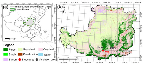
Figure 1.
Location of the study area. (a) The position of the Loess Plateau; (b) The locations of Yongshou (YS), Zhengning (ZN), and Baishui (BS).
2.2. Acquisition and Preprocessing of UAV Multispectral and Landsat Remote Sensing Data
2.2.1. UAV Platform and Multispectral Sensor
The DJI Phantom 4 Multispectral is a survey UAV equipped with an integrated multispectral imaging system designed for high-precision multispectral data collection. Renowned for its user-friendly design, this UAV is depicted in Figure 2. It includes a unique imaging system consisting of an RGB camera and multiple spectral band sensors—blue, green, red, near-infrared (NIR), and red edge. The incorporation of an RTK module together with the DJI TimeSync system allows for precise location data acquisition. This combination ensures centimeter-level positioning accuracy and makes it easy to capture accurate RGB and multispectral images.
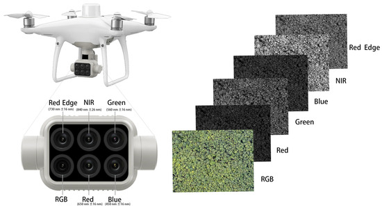
Figure 2.
Unmanned aerial vehicle (UAV) platform and multispectral sensor.
2.2.2. Setting up the UAV Operation Plots
Multispectral data from UAVs were collected in the forested area of Yongshou County under clear, cloudless weather conditions. The survey plots were strategically positioned throughout the study area to ensure uniform distribution and precise localization. These positions were determined by examining both the topographical layout of the county and the spatial distribution data for various tree species; the latter were obtained from the National Forest Resources Inventory (NFRI) Type-II data source. Using these detailed data and employing supervised learning, we predefined the distribution areas of coniferous and broadleaf forests, which are explicitly marked with their specific locations and spatial extents in Figure 3c. Considering the characteristics of the forest areas in the county, where coniferous and broadleaf forests appear in large clusters and small, dispersed patches, this study designed an appropriate flight operation plan. Specifically, smaller plots (shown in Figure 3a) were labeled P1 to P17, while larger plots (depicted in Figure 3b,d) were named P18 and P19. Plots P1 to P8 and P18 were designated as broadleaf forest plots, and P9 to P17 and P19 were designated coniferous forest plots.
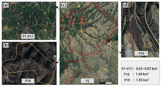
Figure 3.
Distribution of UAV multispectral sample plots: (a) distribution of scattered small plots; (b) distribution of large-block plots; (c) distribution of plots in YS County; and (d) distribution of large-block plot distribution. “P” represents “plot”.
2.2.3. UAV Operation Parameters and Data Preprocessing
Details regarding the UAV flight, including the date, time, and total number of images captured, are documented in Table 1. The UAV was programmed to fly at an altitude of 100 m, achieving a ground resolution of 0.13 m. It maintained forward and side overlap rates of 80% and 75%, respectively, and captured images at 2 s intervals.

Table 1.
Unmanned aerial vehicle (UAV) multispectral data operation parameters.
For radiometric calibration, this study employed a diffuse reflectance board in conjunction with GS Pro software version 2.5.3 (developed by DJI Innovations, based in Shenzhen, China) and Terra v2.3.3 software (also from DJI Innovations). The radiometric calibration is detailed in Figure S1a, with the following reflectance coefficients: blue at 0.65, green at 0.66, red at 0.66, red edge at 0.65, and NIR at 0.59. Using Terra v2.3.3 software, this study generated orthoimages for all plots, which also facilitated atmospheric and reflectance corrections. To perform the geometric calibration, nine targets with unique markers were strategically placed within the UAV operating area, and their locations were accurately recorded using a handheld RTK device (manufactured by South Surveying, Guangzhou, China), as shown in Figure S1b. The coordinates of these targets were entered into the software to calibrate the system, with Figure S1c illustrating the comparison of images before and after target-based correction. The process culminated in the acquisition of the final multispectral composite data shown in Figure 4.
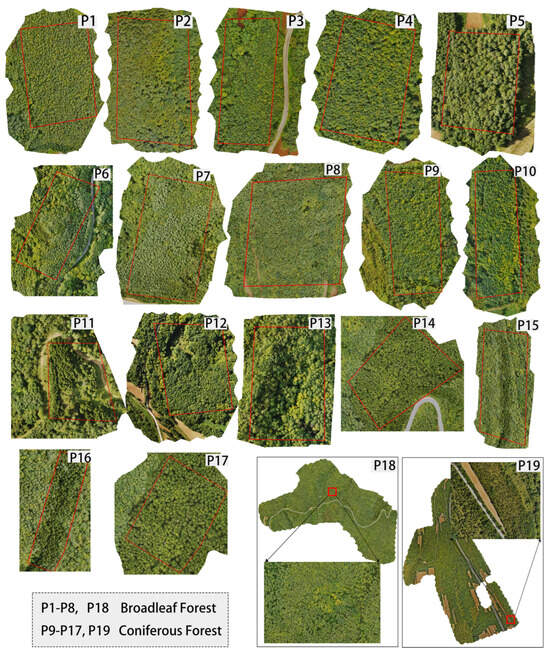
Figure 4.
UAV multispectral data of coniferous and broadleaf forest plots based on multispectral synthesis.
2.2.4. Acquisition and Preprocessing of Landsat Remote Sensing Images
To minimize the variability in data characteristics caused by differences in acquisition months, this study selected Landsat Operational Land Imager (OLI) remote sensing images from the same months as the unmanned aerial vehicle (UAV) multispectral data collection. These images, with less than 5% cloud cover (Figure S2), were sourced from the U.S. Geological Survey website (https://earthexplorer.usgs.gov/, accessed on 4 March 2023). The basic information involved in the research is recorded in Table 2. All images underwent preprocessing steps such as radiometric calibration, atmospheric correction, geometric correction, cropping, and mosaicking. Specifically, geometric correction was performed using high-resolution Gaofen-2 panchromatic images for orthorectification of the Landsat OLI images in ENVI 5.3 software, with a calibration error of 0.12 pixels.

Table 2.
Data related to the Landsat images.
2.3. Rapid Identification of Broadleaf and Coniferous Forests Using Deep Learning-Based Techniques
As illustrated in Figure 5, this study developed a deep learning-based technique to rapidly identify extensive areas of coniferous and broadleaf forests on the Loess Plateau. Additionally, this study conducted a comprehensive sensitivity analysis of the model to reveal how key factors such as image size, sample quantity, and model depth impact model performance. The entire process is based on pre-training the model using a large, pre-acquired dataset. Subsequently, the model is fine-tuned using transfer learning techniques on a smaller dataset of UAV multispectral imagery. This approach allows us to evaluate performance changes before and after fine-tuning the pre-trained model.
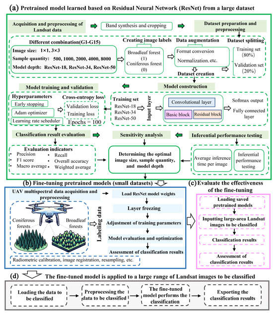
Figure 5.
The framework for identifying broadleaf and coniferous forests using Residual Neural Network (ResNet) architecture and transfer learning techniques: (a) pre-trained model; (b) fine-tuning the pre-trained model; (c) evaluation of the effectiveness of the fine-tuning; and (d) model application.
2.3.1. Dataset Preparation for Labeling
The labeled dataset for the input model in this study comprises two parts: a large dataset for pre-training the model and a smaller dataset for fine-tuning the model. Based on the coniferous and broadleaf forest vector boundaries provided by the NFRI Type-II data, sample labels are extracted from Landsat images using window sizes of 1 × 1 and 3 × 3 pixels. Labels for broadleaf forests are marked as ‘1’, and for coniferous forests as ‘0’. This step aims to accurately capture the spectral texture information of the corresponding samples. The generated images have sizes of 0.0009 km2 and 0.0081 km2, with sample quantities of 500, 1000, 2000, 4000, and 8000, respectively. The smaller dataset consists of multispectral data from UAVs, used for fine-tuning the model. Its spatial resolution is adjusted to match that of the large dataset through the Spectral Angle Mapper technique. Each 0.0009 km2 grid cell is independently labeled. The final dataset contains 288 labels for coniferous forests and 320 for broadleaf forests. These data are processed using ArcMap 10.5 software to ensure consistency and accurate label assignment.
2.3.2. Determining the Number of Input Channels for the Model
To optimize the use of pre-trained weights and to reduce the need to relearn features during the fine-tuning phase, this study ensures that the number of data channels remains consistent throughout the pre-training and fine-tuning phases. This consistency facilitates faster model convergence and improves the overall performance of the final model. In selecting an appropriate combination of channels, this study considered the spectral bands common to both Landsat and UAV multispectral data, specifically the red, green, blue, and NIR bands. Additionally, the choice of three-band combinations was influenced by the architecture of the ResNet model, which is inherently designed to handle three-channel inputs. A random forest algorithm was employed to assess the classification accuracy levels of various band combinations. The results, displayed in Figure S3, indicate that the combination including the NIR band (GBNir: green, blue, and NIR) outperforms other combinations in classification accuracy on both data sources, consistently achieving accuracies above 0.79. This superior performance suggests that the GBNir combination provides a richer and more discriminative set of information, making it the preferred choice for the input channels of the model. As a result, the GBNir band combination was selected as the default input configuration for ongoing model training and transfer learning efforts.
2.3.3. Constructing Pre-Trained Models
- (1)
- Model Selection
ResNets are a prominent architecture in the field of deep learning which have been widely used for image processing and recognition tasks. Introduced by [39], the innovative aspect of ResNet is its use of residual learning to address the vanishing gradient problem which is common in deep networks training. In this study, ResNets of different depths are used: ResNet-18, ResNet-34, and ResNet-50. As shown in Table 3, ResNet-18 and ResNet-34 consist of 18 and 34 layers, respectively, and feature a standard stacked structure of residue blocks. Each block comprises two convolutional layers; specifically, ResNet-18 includes 8 such blocks, while ResNet-34 contains 16.

Table 3.
Residual Neural Network (ResNet) model structure.
ResNet-50, on the other hand, adopts a deeper structure, with 50 layers, and utilizes a ‘bottleneck’ design in its blocks. Each bottleneck block consists of a 1 × 1 convolution for dimension reduction, a 3 × 3 convolution for feature extraction, and another 1 × 1 convolution for dimension recovery. This configuration not only reduces the parameter count but also enhances the depth of feature extraction.
For specific image sizes (1 × 1 and 3 × 3), the kernel size and stride of the initial convolution layer are adjusted, and the pooling layer is removed. These modifications prevent premature shrinkage of feature maps and the loss of essential spatial information, thus ensuring the efficiency and performance of the model when processing images of specific dimensions.
- (2)
- ResNet Model Initialization and Architectural Adjustments
The selected ResNet models are initialized using the PyTorch deep learning framework. All weights are initialized using He normal initialization, and biases are set to zero to ensure training stability. The architecture is further adjusted by modifying the final fully connected layer. Originally designed to output 1000 neurons, this layer is altered to produce only two neurons to meet the specific classification needs of the two of image types: coniferous and broadleaf forests.
- (3)
- Training of ResNet Models
We employed ResNet models of varying depths (ResNet-18, ResNet-34, and ResNet-50) as the foundational architecture, training them using the prepared large dataset (Landsat labeled data). To meet the input requirements of the ResNet models, the images were maintained at uniform sizes (1 × 1 and 3 × 3 pixels) and normalized to minimize the effects of lighting and shadows. Initial training involved preliminary runs on this large dataset. Determining the optimal combination of hyperparameters required iterative adjustments and trials [40]. Various parameters were tested, with the initial learning rate set at 0.01, using the Adam optimizer, and employing the He normal distribution for weight initialization to promote early convergence. Weight decay (L2 regularization) was applied at 0.0001, and the ReLU function was selected as the activation function; dropout techniques were not employed. This study utilized the cosine annealing learning rate scheduler, setting the cycle T_max at 100 iterations and the minimum learning rate at 1e-6. Training was terminated early, using the early-stopping method, if there was no improvement in the performance of the validation set after five consecutive iterations, to prevent overfitting. The entire training process spanned 100 epochs, with an 80:20 split between training and test sets, and 10% of the training set reserved for validation.
The model training and fine-tuning processes were conducted on a computer equipped with an Intel Core i7-9700 CPU @ 3.00 GHz and 16 GB of RAM sourced from Intel Corporation, Santa Clara, CA, USA, and running Windows 10, version 22H2. This setup provided a stable software environment for all training and data processing tasks, which were executed within a Python environment. The specific versions of Python and the libraries were installed and configured according to PyTorch’s requirements. Necessary Python libraries such as GDAL, NumPy, Matplotlib, and PyTorch, along with other relevant libraries for remote sensing data processing and deep learning, were installed using Conda and pip. All datasets were stored in TIFF format.
- (4)
- Performance Evaluation of the Pre-trained Model
The performance evaluation of the model is conducted across three dimensions: stability, classification accuracy, and time efficiency. First, to assess stability of the model, this study utilizes training curves, a tool vital in monitoring the learning process. These curves display the loss values for each training epoch, helping to analyze trends in loss reduction across both the training and validation sets. This analysis indicates whether the model is overfitting or underfitting. An ideal training curve should exhibit a trend of gradually decreasing loss values that stabilize over time, suggesting effective learning without overfitting [41].
Next, this study asses the time efficiency of the ResNet models, focusing on two core metrics: total training time and average inference time per image. Total training time, measured in hours, indicates the duration required for the model to progress from initialization to completion of specified training epochs. This metric reflects the time cost necessary for the model to achieve a certain level of performance. The average inference time per image, measured in seconds, assesses how quickly the model can process a new image input and output a prediction [42].
Finally, regarding the classification accuracy of the model, this study introduces a series of key performance indicators: accuracy, recall, precision, and F1-score. These metrics are calculated based on the confusion matrix of the binary classification problem. In this matrix, as shown in Table 4, rows represent the actual class samples, while columns represent the classes predicted by the model. Table 5 further provides the mathematical expressions for these performance metrics.

Table 4.
Binary classification confusion matrix.

Table 5.
The performance metrics.
2.3.4. Sensitivity Analysis
In this study, experimental analyses are conducted across three critical dimensions: image size, sample quantity, and model depth. Fifteen different training strategy combinations were established to cover a range of possible configurations for analyzing model sensitivity, with detailed parameters as presented in Table 6. By conducting a comprehensive performance evaluation for each model combination, the optimal strategy combination was determined in order to ensure both the accuracy and the efficiency of the classification results.

Table 6.
Different combinations of strategies.
2.3.5. Fine-Tuning the Pre-Trained Model Using Transfer Learning and Performance Evaluation
After the construction and initial training of the pre-trained model, this study then fine-tunes it using a small, specially prepared dataset of labeled multispectral UAV data. The objective of this phase is to adjust and optimize the model’s parameters to enhance its responsiveness and classification accuracy with the new dataset. To ensure consistency, the input format of the UAV-labeled dataset matches that used in the pre-trained model. The weights of the pre-trained ResNet model are loaded using the DataLoader function within the PyTorch framework. For fine-tuning, the learning rate is set to 0.001, while other hyperparameters remain unchanged. Notably, a dropout rate of 0.5 is added to the final fully connected layer to enhance the model’s generalization capability. Early stopping is implemented with a patience of three rounds, and the number of fine-tuning training rounds is limited to 10. The loss function employed is cross-entropy loss, maintaining an 80:20 data ratio for training and testing. Figure 5c,d illustrate the steps for assessing the effectiveness and broad applicability of the model after fine-tuning. The study area’s data awaiting classification is applied to both the fine-tuned model (Figure 5b) and the directly trained ResNet model (Figure 5a), using a wide range of data. The validated and fine-tuned models are then applied to Baishui County and Zhengning County, comparing classification accuracies to observe the model’s suitability.
3. Results
3.1. Impacts of Different Combination Strategies on the Performance of Pre-Trained Models
This study evaluated the performance of pre-trained models using metrics across three dimensions, namely, loss curve, time efficiency, and classification accuracy, aiming to investigate how image size, sample quantity, and model depth—three critical factors—affect model performance. The experimental design was organized into two groups based on image sizes: the first group utilized 1 × 1 images, while the second employed 3 × 3 images. Furthermore, this investigation encompassed a range of sample quantities (from 500 to 8000) and model depths (from ResNet-18 to ResNet-50) to determine the impacts of various combination strategies on model performance.
3.1.1. Loss-Curve Variation Trends
The loss curve is a metric pivotal for gauging the performance of pre-trained models, providing a vivid visual representation of the model’s learning journey and stability during training. This research delves into the effects of varying image sizes on the training efficacy of deep learning models by examining the loss curves based on images of 1 × 1 and 3 × 3 pixels. To evaluate the influences of various factors on model performance, the study employed strategies that incorporated a diverse range of sample quantities (500, 1000, 2000, 4000, and 8000) and model depths (ResNet-18, ResNet-34, and ResNet-50). These strategies were designed to monitor loss changes across both training and validation datasets in order to understand the impacts of these factors on the model’s training outcomes.
The results shown in Figure 6 reveal that within the 1 × 1 image configuration, the majority of combination strategies (G7–G15) exhibit a decline in both training and validation loss curves as the epoch count increases. Notably, the rate of decrease in training loss generally surpasses that of validation loss, indicating the model’s ability to learn effectively from the training data. However, certain combination strategies (G1–G6) display either fluctuating trends or a minor upward trend in their validation loss-curves. Conversely, under the 3 × 3 image configuration depicted in Figure 7, the loss curves display more uniform fluctuations and a more consistent downward trend, particularly with respect to the training loss. This suggests that the model exhibits enhanced generalization capabilities and a reduced likelihood of overfitting when processing information across a broader context. Further examination of the 1 × 1 image configuration shows that the validation loss-curves tend to stabilize with increasing sample size, underscoring the beneficial impacts of appropriate sample sizes on the model’s generalization ability. Additionally, the selection of model depth substantially affects the loss curves’ dynamics and the model’s ability to mitigate overfitting, highlighting effective adaptive strategies for various model depths. In contrast, for the 3 × 3 image configuration, a moderate sample size of 2000 (G7–G9) leads to a markedly consistent decline and minimal volatility in the model’s loss curves, demonstrating improved generalization performance in this specific setup.
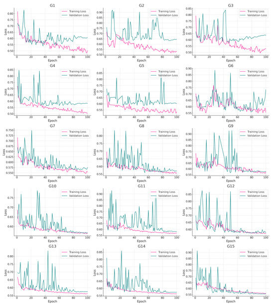
Figure 6.
Trends associated with loss-curve changes under different combination strategies, with a 1 × 1 window size.
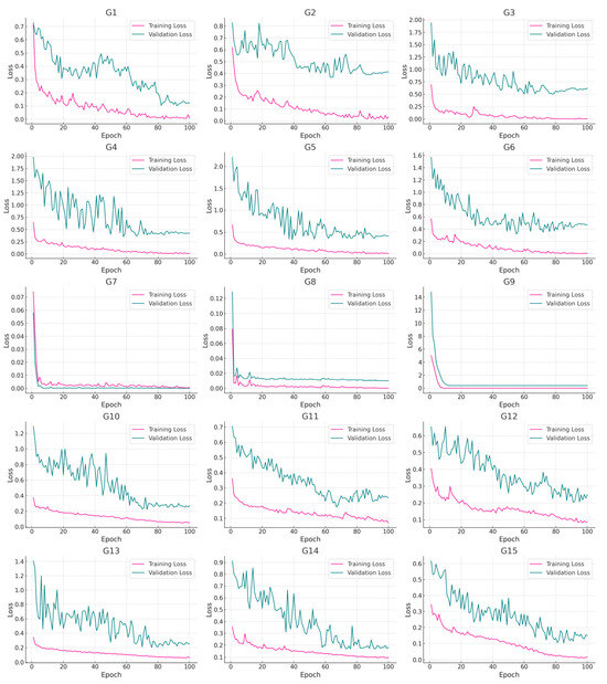
Figure 7.
Trends associated with loss-curve changes under different combination strategies, with a 3 × 3 window size.
In a side-by-side analysis of the loss curves for 1 × 1 and 3 × 3 image settings, it becomes clear that the 3 × 3 configuration achieves a quicker stabilization. This indicates that slightly larger image sizes are more effective in capturing a wider spectrum of information, which helps the model recognize more intricate data features and improves its ability to generalize on the validation set. While the 1 × 1 setting might show a slower rate of loss reduction, it offers long-term benefits by lowering the likelihood of overfitting, thus boosting the model’s consistency and dependability. Moreover, the 1 × 1 setup is particularly sensitive to sample quantity and model depth. An increase in model depth highlighted the crucial role of having enough samples for generalization, revealing a distinct pattern. On the other hand, with the 3 × 3 configuration, there are noticeable disparities in how quickly and smoothly the loss curve declines; both factors are influenced by both model depth and the quality of the samples.
3.1.2. The Impacts of Image Size, Sample Quantity, and Model Depth on the Time Efficiency of Pre-Trained Models
Figure 8 reveals how image size, sample quantity, and model depth impact both the overall training time and average inference time per image for ResNet models. When comparing total training times, it is evident that using an image size of 1 × 1 extends training significantly, compared to use of 3 × 3, suggesting minimal gains in computational efficiency from reducing image size. There was a noticeable escalation in training time which occurred as the sample quantity grew, particularly from 500 to 2000 samples, with the rate of increase becoming more moderate between 4000 and 8000 samples. Model depth also played a role in training time, with ResNet-50 requiring much longer training periods than both ResNet-18 and ResNet-34. Remarkably, ResNet-34 achieved the shortest overall training time, indicating that a network of moderate complexity can offer substantial time savings. With respect to the average inference time per image, the trend was similar to that of the overall training times, showing that 3 × 3 images are processed more efficiently during inference than are their 1 × 1 counterparts. Apart from the highest sample quantity of 8000, an increase in sample quantity led to a notable rise in inference time, suggesting that efficiently processing diverse dataset sizes is feasible once the model is adequately trained. Nevertheless, as the model depth increased, so did inference time, particularly with ResNet-50, underscoring the increased computational demands of deeper models during inference. To summarize, image size, sample quantity, and model depth substantially shape the computational efficiency of models.
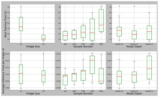
Figure 8.
Impacts of image size, sample quantity, and model depth on the total training time and the average inference time per image of the residual architecture model.
3.1.3. The Impacts of Image Size, Sample Quantity, and Model Depth on Classification Results
To evaluate the performance of different combination strategies on the forest-type classification task, this study focused on assessing the effects of these variables on the following six performance indicators: accuracy, recall, F1-score, overall accuracy, macro average, and weighted average.
Figure 9 reveals that appropriate image sizes, specifically 3 × 3, consistently achieve higher precision and recall in classifying coniferous and broadleaf forests, particularly when sample sizes increase. This emphasizes the critical roles of a wider viewing perspective and a more comprehensive training dataset in accurately identifying specific types of forests. An upward trend in F1-score, along with improvements in precision and recall, indicates that enlarging image dimensions and increasing sample quantities can balance these metrics effectively, thereby enhancing the model’s overall performance. This increase in model precision, brought about by bigger image sizes and more samples, highlights the value of broader contextual data and plentiful training examples in improving classification accuracy. Comprehensive performance metrics, such as the macro and weighted averages, show the model’s consistent performance improvement across all categories. This progress, reflected in the rise of overall precision, further validates the effectiveness of increasing both image size and sample quantity in boosting model capabilities. Notably, under the conditions of 3 × 3 image sizes and a dataset of 2000 samples, the highest accuracy was achieved by employing strategies with three different model depths, namely, G7, G8, and G9. To summarize, the study showcases the influences of different combination strategies on model efficiency, revealing that, although model performance benefits from increased depth and sample size with 1 × 1 images, the optimal outcome is seen with 3 × 3 images and a sample quantity of 2000.
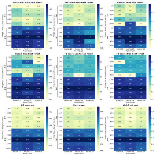
Figure 9.
Differences in classification results of coniferous and broadleaf forests among different combination strategies.
Overall, the image size substantially impacts model accuracy. Specifically, increasing the image size from 1 × 1 to 3 × 3 enhances performance across most combinations of sample sizes and model depths. This result indicates that appropriate images offer more contextual information, which aids in the model’s feature-recognition capabilities across different forest types. Furthermore, the number of training samples plays a crucial role in the model’s classification accuracy. As training samples increase, so does accuracy in distinguishing between the two types of forests. This trend is especially evident at sample sizes of 2000, 4000, and 8000, emphasizing the need for substantial training data to improve model generalization. Additionally, the analysis of model depth reveals that, in scenarios with smaller images (1 × 1) and fewer samples, simpler models like ResNet-18 can sometimes outperform deeper models such as ResNet-50. However, as image sizes and sample quantity grow, the advanced feature extraction and representation capabilities of deeper models generally yield better performance.
These insights highlight the critical role of factors like image size, sample quantity, and model depth in optimizing pre-trained models for specific tasks. Image size and sample size are crucial for enhancing model classification accuracy, while the choice of model depth should be flexibly determined based on the specific requirements of the task and the characteristics of the data.
3.2. Fine-Tuning Pre-Trained Models with Multispectral UAV Data for Enhanced Classification Performance
Following the evaluation of model performance and repeated testing of combination strategies, G9 was identified as the optimal strategy for inputting data into the pre-trained model. Based on pre-trained models, this study examined the accuracy of forest-type classification results before and after fine-tuning with UAV multispectral data. Additionally, this research selected two counties with forest types similar to Yongshou County, Zhengning County and Baishui County, to assess and ensure the robustness and general applicability of the model by applying it to these three counties.
Figure 10 displays the spatial distribution maps of coniferous and broadleaf forests in the three counties, with the classification accuracy shown in Table 7. The accuracy in Zhengning increased from 85% to 93%; in Yongshou, from 89% to 96%; and in Baishui, from 86% to 94%. These results indicate that fine-tuning the model is very effective in improving the accuracy of forest-type classification. The accuracy in all areas reached or exceeded the 90% threshold after fine-tuning, demonstrating the robustness and applicability of the adopted method under various terrain types and ecological conditions. These findings contribute valuable experimental evidence aiding the further optimization of remote sensing image analysis, offering scientific guidance for precision forest management and the planning of sustainable development.
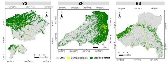
Figure 10.
Spatial distribution map of coniferous and broadleaf forests.

Table 7.
Precision comparison before and after fine tuning of the pre-model.
4. Discussion
This study aimed to achieve two primary objectives, namely, to develop an effective technical framework for rapidly distinguishing forest types using deep learning technology combined with multisource remote sensing data, and to reveal the impacts of image size, sample quantity, and model depth on the time efficiency and accuracy of the training model. This research not only offers new perspectives and methods for forest landscape classification at the technical level but also provides effective technical support for forest management and environmental monitoring in the Loess Plateau.
This framework introduces a fine-tuning-based transfer learning strategy that effectively integrates cross-scale information sources (UAV multispectral data and Landsat remote sensing data), which significantly enhances the overall accuracy and efficiency of large-scale forest-type identification in the region. This improvement is likely due to the rigorous adherence to the fine-tuning-based transfer learning strategy, one which effectively addresses the issue of insufficient training data for deep neural networks [43,44]. First, knowledge from one or more source tasks is acquired during the pre-training phase, and then this knowledge is transferred to the target task during the fine-tuning phase. The rich knowledge acquired in the pre-training phase enables the model to effectively handle the target task with limited samples during the fine-tuning phase [45]. The technical framework proposed in this study consists of three important components: the pre-trained model, the fine-tuned model, and the application to a wide range of data awaiting classification. The pre-trained and fine-tuned models, as the core parts of the entire framework, are especially beneficial for achieving advanced results in image classification when the target tasks in both phases are the same [16]. In recent years, some studies have successfully identified forest tree species and achieved good classification results by adopting advanced deep learning architectures [20,27,46]; other scholars have also recognized forest tree species by applying transfer learning strategies [47,48,49]. While these specific classification tasks employ models such as fine-tuned transfer learning, they often overlook the quality and relevance of the metadata sets in the pre-training steps. Existing research indicates that if the source dataset differs substantially from the target application scenario, the model’s effectiveness might be limited [16,22]. Our study does not rely solely on the original image datasets in deep architectural models, but instead uses a large Landsat labeled dataset for training the model. Only after validating the model’s performance does this study use small-scale UAV labeled data for fine-tuning, taking full advantage of the hierarchical structure of the deep architectural model. Our results also confirm the maturity of our technical framework model, which achieves or exceeds a 90% accuracy threshold in all areas tested. This result not only demonstrates the effectiveness of the methods employed, but also underscores their reliability across different terrains and ecological conditions.
Selecting an appropriate image size for specific application scenarios and resource limitations and adjusting the data preprocessing workflow and model structure accordingly can more effectively balance size and performance [50,51]. The majority of deep convolutional neural networks, particularly those based on the ResNet model, are generally designed to handle deep learning tasks involving images with widths and heights ranging from tens to hundreds of pixels [52]. This design aims to capture visual features sufficient for effective learning and prediction [53]. Many readily available deep learning models and pre-trained weights are based on standard image sizes (224 × 224 pixels). In this study, to accurately reflect the impact of image size variations, the configuration of the model’s input layer was adjusted while keeping other conditions such as model architecture, training epochs, and learning rate unchanged. The performance of the loss curves in Figure 6 and Figure 7 demonstrates that images with dimensions of 1 × 1 or 3 × 3 pixels carry feature information sufficient to meet the model’s effectiveness and performance requirements. This indicates that for deep residual network models, satisfactory results can be achieved in terms of model performance for specific applications, even when using particular image sizes [54,55]. However, given the limited availability of samples from remote sensing data sources, whether a labeled dataset constructed with appropriate image sizes can enhance the model’s generalization capability and stability remains a topic for debate. Further research should aim to explore and optimize the integration of multisource remote sensing data using deep learning technologies to improve the spatial resolution of medium to low-resolution (Landsat) imagery. Although data augmentation and preprocessing techniques can effectively increase the sample quantity and ensure model stability, they cannot completely eliminate the potential negative impact of augmented samples on the model’s generalization ability. Therefore, further improvements are needed to enhance the interpretability of deep residual architecture models. Moreover, attention should be paid to increasing the efficiency and reducing the cost of genuine sample data collection, and more diverse model optimization strategies should be explored to further enhance the generalizability and practicality of the model. Additionally, investigating the application of these technologies on a global scale can provide more comprehensive support for environmental monitoring and forest management. This study has effectively improved the identification accuracy and efficiency of coniferous and broadleaf forests in the Loess Plateau by combining deep learning with multisource remote sensing data, paving a new path for the application of remote sensing technology in forest management and environmental monitoring.
Effectively quantifying and identifying factors that impact the performance of ResNet models is crucial for model interpretability [56,57]. In our study, we selected image size, sample quantity, and model depth as the three potential influencing factors for study, evaluating their impacts on the model through meticulously designed experiments. Unlike previous studies [56,58], this research focuses not only on the influence of individual factors, but also systematically examines the combined effects of these factors. The experiments comprised fifteen different combination strategies (Table 6) to test their responsiveness to model performance. To comprehensively assess the model, this study employed a robust evaluation of performance across three dimensions, namely, stability, accuracy, and time efficiency, ultimately determining the model’s optimal combination strategy (G9). Our study highlights the substantial impacts of different combination strategies (including model depth, sample quantity, and image size) on the performance of forest-type classification tasks. It also emphasizes the importance of considering these factors—image size, sample quantity, and model depth—in the design and optimization of pre-trained models. Image size and sample quantity are key factors in enhancing model classification accuracy, while the choice of model depth should be flexibly determined based on the specific requirements of the task and the characteristics of the data, a determination which is consistent with the views of existing studies [59,60,61]. Moreover, these factors substantially affect the time efficiency of model training and inference, which is particularly important in resource-constrained application scenarios. In summary, for optimal performance and efficiency, model design should carefully balance these factors, based on the specific task and available resources.
Although this study provides an effective method for classifying forest types on the Loess Plateau, there may still be issues with the singularity of the data sources. The limited coverage of UAV data and the spatial resolution constraints of Landsat data could affect the accuracy and representativeness of the study results. Additionally, the choices of sample quantity and study area may limit the generalizability of the findings. If the sample size is insufficient or the selected study area does not represent the diversity of the entire Loess Plateau region, the model’s generalization ability may be compromised. Using the ResNet model and transfer learning techniques can improve classification accuracy, but it also increases the model’s complexity and computational cost. In practical applications, this complexity might limit the model’s usability and practicality. Although the study evaluated different spectral band combinations, it may not have covered all possible combinations. For certain vegetation types, specific spectral information might be required to achieve optimal classification results. Moreover, the study may not have fully considered the impacts of seasonal and climatic changes on the spectral characteristics of vegetation. Vegetation spectral responses can vary under different seasonal and climatic conditions, thereby influencing classification results. Despite these limitations, the model can be adjusted and optimized through transfer learning, as long as corresponding remote sensing data and sufficient samples are available.
Our research is only a first step towards cross-scale forest monitoring. Future studies may extend upon this technical foundation using UAV hyperspectral and LiDAR data. By enriching spectral features and spatial information, these studies could further achieve large-scale tree species classification on the Loess Plateau, a process critically important for evaluating vegetation restoration outcomes.
5. Conclusions
This study successfully developed and validated a deep learning classification framework that integrates multispectral UAV data with Landsat remote sensing data to efficiently and accurately identify coniferous and broadleaf forests on Loess Plateau. The following are the key findings:
- By integrating the ResNet architecture with transfer learning techniques, and utilizing multispectral data from UAVs and Landsat satellites, the framework achieved substantial improvements in classification accuracy. The fine-tuned model achieved over 90% accuracy in classifying forest types in Yongshou, Zhengning, and Baishui counties. This validates the effectiveness and rapidity of the proposed technical framework.
- The study systematically evaluated the effects of image size, sample quantity, and model depth on the model’s performance. It was found that appropriate image sizes (3 × 3 pixels) and increased sample quantities substantially enhance the model’s classification accuracy and generalization ability. The optimal strategy was identified as using a 3 × 3 image size, 2000 samples, and a ResNet-50 model depth, achieving the best balance between accuracy and efficiency.
Overall, the research not only validates the effectiveness of deep learning and transfer learning in forest-type classification but also provides an innovative technical path for forest resource monitoring and management. These achievements offer valuable scientific guidance for forest management and sustainable development on the Loess Plateau.
Future research should further explore the integration of additional spectral data and assess the model’s adaptability across different geographical and climatic conditions to fully reveal the potential applications of deep learning technologies in remote sensing.
Supplementary Materials
The following supporting information can be downloaded at: https://www.mdpi.com/article/10.3390/rs16122096/s1, Figure S1: Calibration of UAV multispectral data: (a) Radiometric calibration; (b) Target-laying calibration; (c) Effect before and after target correction. Figure S2: Landsat RGB data with less than 5% cloud cover: (a) YS; (b) ZN; (c) BS. Figure S3: Classification accuracy of different band combinations of Landsat data and UAV data based on the random forest algorithm.
Author Contributions
Conceptualization, M.Z.; Formal analysis, M.Z., D.Y. and Z.L.; Funding acquisition, Z.Z.; Investigation, M.Z., D.Y. and Z.L.; Methodology, D.Y. and Z.L.; Project administration, Z.Z.; Resources, Z.Z.; Software, M.Z., D.Y. and Z.L.; Supervision, Z.Z.; Validation, M.Z. and Z.Z.; Writing—original draft, M.Z.; Writing—review and editing, Z.Z. All authors have read and agreed to the published version of the manuscript.
Funding
This research was funded by the National Key Research and Development Program of China as “Quality improvement technology of low-efficiency plantation forest ecosystem in the Loess Plateau”, grant number 2022YFF1300400; and “The Subject: Multifunctional enhancement of Robinia pseudoacacia forests in hilly and gully areas and techniques for maintaining vegetation stability on the Loess Plateau [grant number 2022YFF1300405]; Special Topic: Distribution Pattern, Causes and Change Trends of Low-Efficiency Robinia pseudoacacia plantations.”
Data Availability Statement
The data supporting the findings of this study are derived from the Second National Forest Resources Inventory specific to YS county, BS county, and ZN county, provided by the Shaanxi Provincial Forestry Bureau. Due to confidentiality agreements, the data cannot be made publicly available. However, researchers seeking access for valid academic purposes can make direct requests to the Shaanxi Provincial Forestry Bureau, subject to their data access and sharing policies.
Acknowledgments
This study would like to extend our sincere gratitude to the Shaanxi Provincial Forestry Bureau for providing us with the data from the Second National Forest Resources Inventory specific to YS county, BS county, and ZN county. This invaluable data significantly underpinned the analyses and findings of our study. Our deepest gratitude goes to the editors and reviewers for their careful work and thoughtful suggestions.
Conflicts of Interest
This study involved no competing financial interest or personal relationships that could have appeared to influence the work reported in this paper.
References
- Locatelli, B. Ecosystem services and climate change. In Routledge Handbook of Ecosystem Services; Routledge: London, UK, 2016; pp. 481–490. [Google Scholar] [CrossRef]
- Sultana, F.; Arfin-Khan, M.; Karim, M.; Mukul, S. Rainfall Modifies the Disturbance Effects on Regulating Ecosystem Services in Tropical Forests of Bangladesh. Forests 2023, 14, 272. [Google Scholar] [CrossRef]
- Kramer, K.; Leinonen, I.; Loustau, D. The importance of phenology for the evaluation of impact of climate change on growth of boreal, temperate and Mediterranean forests ecosystems: An overview. Int. J. Biometeorol. 2000, 44, 67–75. [Google Scholar] [CrossRef] [PubMed]
- Walkiewicz, A.; Bieganowski, A.; Rafalska, A.; Khalil, M.; Osborne, B. Contrasting Effects of Forest Type and Stand Age on Soil Microbial Activities: An Analysis of Local Scale Variability. Biology 2021, 10, 850. [Google Scholar] [CrossRef] [PubMed]
- Gao, L.; Bowker, M.; Xu, M.; Sun, H.; Tuo, D.; Zhao, Y. Biological soil crusts decrease erodibility by modifying inherent soil properties on the Loess Plateau, China. Soil Biol. Biochem. 2017, 105, 49–58. [Google Scholar] [CrossRef]
- Lu, A.; Tian, P.; Mu, X.; Zhao, G.; Feng, Q.; Guo, J.; Xu, W. Fuzzy Logic Modeling of Land Degradation in a Loess Plateau Watershed, China. Remote Sens. 2022, 14, 4779. [Google Scholar] [CrossRef]
- Liu, J.; Chang, Q.; Zhang, J.; Chen, T.; Jia, K. Effect of vegetation on soil fertility in different woodlands on Loess Plateau. J. Northwest A F Univ. Nat. Sci. Ed. 2004, 32, 111–115. [Google Scholar] [CrossRef]
- Huang, Y.; Liu, D.; An, S. Effects of slope aspect on soil nitrogen and microbial properties in the Chinese Loess region. Catena 2015, 125, 135–145. [Google Scholar] [CrossRef]
- Shi, Z.; Bai, Z.; Guo, D.; Chen, M. Develop a Soil Quality Index to Study the Results of Black Locust on Soil Quality below Different Allocation Patterns. Land 2021, 10, 785. [Google Scholar] [CrossRef]
- Lehmann, E.A.; Caccetta, P.; Lowell, K.; Mitchell, A.; Zhou, Z.S.; Held, A.; Tapley, I. SAR and optical remote sensing: Assessment of complementarity and interoperability in the context of a large-scale operational forest monitoring system. Remote Sens. Environ. 2015, 156, 335–348. [Google Scholar] [CrossRef]
- Lu, M.; Chen, B.; Liao, X.H.; Yue, T.X.; Yue, H.Y.; Ren, S.M.; Xu, B. Forest types classification based on multi-source data fusion. Remote Sens. 2017, 9, 1153. [Google Scholar] [CrossRef]
- Liu, Y.; Gong, W.; Hu, X.; Gong, J. Forest Type Identification with Random Forest Using Sentinel-1A, Sentinel-2A, Multi-Temporal Landsat-8 and DEM Data. Remote Sens. 2018, 10, 946. [Google Scholar] [CrossRef]
- Elizar, E.; Zulkifley, M.A.; Muharar, R.; Zaman, M.H.M.; Mustaza, S.M. A review on multiscale-deep-learning applications. Sensors 2022, 22, 7384. [Google Scholar] [CrossRef] [PubMed]
- Li, J.X.; Hong, D.F.; Gao, L.R.; Yao, J.; Zheng, K.; Zhang, B.; Chanussot, J. Deep learning in multimodal remote sensing data fusion: A comprehensive review. Int. J. Appl. Earth Obs. Geoinf. 2022, 112, 102926. [Google Scholar] [CrossRef]
- Day, O.; Khoshgoftaar, T.M. A survey on heterogeneous transfer learning. J. Big Data 2017, 4, 29. [Google Scholar] [CrossRef]
- Ma, Y.C.; Chen, S.; Ermon, S.; Lobell, D.B. Transfer learning in environmental remote sensing. Remote Sens. Environ. 2024, 301, 113924. [Google Scholar] [CrossRef]
- Han, X.; Zhang, Z.; Ding, N.; Gu, Y.; Liu, X.; Huo, Y.; Zhu, J. Pre-trained models: Past, present and future. AI Open 2021, 2, 225–250. [Google Scholar] [CrossRef]
- Cao, K.; Zhang, X. An Improved Res-UNet Model for Tree Species Classification Using Airborne High-Resolution Images. Remote Sens. 2020, 12, 1128. [Google Scholar] [CrossRef]
- Zhang, C.; Xia, K.; Feng, H.; Yang, Y.; Du, X. Tree species classification using deep learning and RGB optical images obtained by an unmanned aerial vehicle. J. For. Res. 2020, 32, 1879–1888. [Google Scholar] [CrossRef]
- Xi, Z.; Hopkinson, C.; Rood, S.B.; Peddle, D.R. See the forest and the trees: Effective machine and deep learning algorithms for wood filtering and tree species classification from terrestrial laser scanning. ISPRS J. Photogramm. Remote Sens. 2020, 168, 1–16. [Google Scholar] [CrossRef]
- Han, T.; Sánchez-Azofeifa, G. A Deep Learning Time Series Approach for Leaf and Wood Classification from Terrestrial LiDAR Point Clouds. Remote Sens. 2022, 14, 3157. [Google Scholar] [CrossRef]
- Thenmozhi, K.; Reddy, U.S. Crop pest classification based on deep convolutional neural network and transfer learning. Comput. Electron. Agric. 2019, 164, 104906. [Google Scholar] [CrossRef]
- Aldayel, M.; Ykhlef, M.; Al-Nafjan, A. Electroencephalogram-Based Preference Prediction Using Deep Transfer Learning. IEEE Access 2020, 8, 176818–176829. [Google Scholar] [CrossRef]
- Odebiri, O.; Odindi, J.; Mutanga, O. Basic and deep learning models in remote sensing of soil organic carbon estimation: A brief review. Int. J. Appl. Earth Obs. Geoinf. 2021, 102, 102389. [Google Scholar] [CrossRef]
- Veras, H.F.P.; Ferreira, M.P.; da Cunha Neto, E.M.; Figueiredo, E.O.; Dalla Corte, A.P.; Sanquetta, C.R. Fusing multi-season UAS images with convolutional neural networks to map tree species in Amazonian forests. Ecol. Inform. 2022, 71, 101815. [Google Scholar] [CrossRef]
- Scheeres, J.; de Jong, J.; Brede, B.; Brancalion, P.H.; Broadbent, E.N.; Zambrano, A.M.A.; de Almeida, D.R.A. Distinguishing forest types in restored tropical landscapes with UAV-borne LIDAR. Remote Sens. Environ. 2023, 290, 113533. [Google Scholar] [CrossRef]
- Lin, F.C.; Shiu, Y.S.; Wang, P.J.; Wang, U.H.; Lai, J.S.; Chuang, Y.C. A model for forest type identification and forest regeneration monitoring based on deep learning and hyperspectral imagery. Ecol. Inform. 2024, 80, 102507. [Google Scholar] [CrossRef]
- Zhong, Z.; Li, J.; Ma, L.; Jiang, H.; Zhao, H. Deep residual networks for hyperspectral image classification. In Proceedings of the 2017 IEEE IGARSS, Worth, TX, USA, 23–28 July 2017; pp. 1824–1827. [Google Scholar] [CrossRef]
- Bharati, S.; Podder, P.; Mondal, M.; Prasath, V. CO-ResNet: Optimized ResNet model for COVID-19 diagnosis from X-ray images. Int. J. Hybrid Intell. Syst. 2021, 17, 71–85. [Google Scholar] [CrossRef]
- Li, H.; Hu, B.; Li, Q.; Jing, L. CNN-Based Individual Tree Species Classification Using High-Resolution Satellite Imagery and Airborne LiDAR Data. Forests 2021, 12, 1697. [Google Scholar] [CrossRef]
- Susanti, M.; Novita, R.; Permana, I. Application of Residual Network Architecture on COVID-19 Chest X-ray Classification. In Proceedings of the International Symposium on Information Technology and Digital Innovation (ISITDI), Virtual, 27–28 July 2022; pp. 121–125. [Google Scholar] [CrossRef]
- Ghimire, B.R.; Nagai, M.; Tripathi, N.K.; Witayangkurn, A.; Mishara, B.; Sasaki, N. Mapping of Shorea robusta forest using time series MODIS data. Forests 2017, 8, 384. [Google Scholar] [CrossRef]
- Li, L.W.; Li, N.; Lu, D.; Chen, Y. Mapping Moso bamboo forest and its on-year and off-year distribution in a subtropical region using time-series Sentinel-2 and Landsat 8 data. Remote Sens. Environ. 2019, 231, 111265. [Google Scholar] [CrossRef]
- Borlaf-Mena, I.; García-Duro, J.; Santoro, M.; Villard, L.; Badea, O.; Tanase, M.A. Seasonality and directionality effects on radar backscatter are key to identify mountain forest types with Sentinel-1 data. Remote Sens. Environ. 2023, 296, 113728. [Google Scholar] [CrossRef]
- Zhang, J.; Zhang, Y.Y.; Zhou, T.Y.; Sun, Y.; Yang, Z.C.; Zheng, S.L. Research on the identification of land types and tree species in the Engebei ecological demonstration area based on GF-1 remote sensing. Ecol. Inform. 2023, 77, 102242. [Google Scholar] [CrossRef]
- Teixeira, I.; Morais, R.; Sousa, J.; Cunha, A. Deep Learning Models for the Classification of Crops in Aerial Imagery: A Review. Agriculture 2023, 13, 965. [Google Scholar] [CrossRef]
- Zhao, X.; Jing, L.; Zhang, G.; Zhu, Z.; Liu, H.; Ren, S. Object-Oriented Convolutional Neural Network for Forest Stand Classification Based on Multi-Source Data Collaboration. Forests 2024, 15, 529. [Google Scholar] [CrossRef]
- Zhen, J.; Mao, D.; Shen, Z.; Zhao, D.; Xu, Y.; Wang, J.; Ren, C. Performance of XGBoost Ensemble Learning Algorithm for Mangrove Species Classification with Multi-Source Spaceborne Remote Sensing Data. J. Remote Sens. 2024, 0146. [Google Scholar] [CrossRef]
- He, K.; Zhang, X.; Ren, S.; Sun, J. Deep residual learning for image recognition. In Proceedings of the IEEE Conference on Computer Vision and Pattern Recognition, Las Vegas, NV, USA, 27–30 June 2016; pp. 770–778. [Google Scholar] [CrossRef]
- Ding, Y.; Sheng, L.; Liang, J.; Zheng, A.; He, R. ProxyMix: Proxy-based mixup training with label refinery for source-free domain adaptation. Neural Netw. 2023, 167, 92–103. [Google Scholar] [CrossRef] [PubMed]
- Salman, S.; Liu, X. Overfitting mechanism and avoidance in deep neural networks. arXiv 2019, arXiv:1901.06566. [Google Scholar] [CrossRef]
- Wu, S.; Li, G.Q.; Chen, F.; Shi, L.P. Training and inference with integers in deep neural networks. arXiv 2018, arXiv:1802.04680. [Google Scholar] [CrossRef]
- Tong, X.Y.; Xia, G.S.; Lu, Q.; Shen, H.; Li, S.; You, S.; Zhang, L. Land-cover classification with high-resolution remote sensing images using transferable deep models. Remote Sens. Environ. 2020, 237, 111322. [Google Scholar] [CrossRef]
- Peng, M.; Liu, Y.; Khan, A.; Ahmed, B.; Sarker, S.K.; Ghadi, Y.Y.; Ali, Y.A. Crop monitoring using remote sensing land use and land change data: Comparative analysis of deep learning methods using pre-trained CNN models. Big Data Res. 2024, 36, 100448. [Google Scholar] [CrossRef]
- Liu, Z.; Xu, Y.; Xu, Y.; Qian, Q.; Li, H.; Ji, X.; Jin, R. Improved fine-tuning by better leveraging pre-training data. Adv. Neural Inf. Process. Syst. 2022, 35, 32568–32581. [Google Scholar]
- Dey, B.; Ahmed, R.; Ferdous, J.; Haque, M.M.U.; Khatun, R.; Hasan, F.E.; Uddin, S.N. Automated plant species identification from the stomata images using deep neural network: A study of selected mangrove and freshwater swamp forest tree species of Bangladesh. Ecol. Inform. 2023, 75, 102128. [Google Scholar] [CrossRef]
- Hamrouni, Y.; Paillassa, E.; Chéret, V.; Monteil, C.; Sheeren, D. From local to global: A transfer learning-based approach for mapping poplar plantations at national scale using Sentinel-2. ISPRS J. Photogramm. Remote Sens. 2021, 171, 76–100. [Google Scholar] [CrossRef]
- Kırbaş, İ.; Çifci, A. An effective and fast solution for classification of wood species: A deep transfer learning approach. Ecol. Inform. 2022, 69, 101633. [Google Scholar] [CrossRef]
- Moritake, K.; Cabezas, M.; Nhung, T.T.C.; Caceres, M.L.L.; Diez, Y. Sub-alpine shrub classification using UAV images: Performance of human observers vs DL classifiers. Ecol. Inform. 2024, 80, 102462. [Google Scholar] [CrossRef]
- Han, D.; Liu, Q.; Fan, W. A new image classification method using CNN transfer learning and web data augmentation. Expert Syst. Appl. 2018, 95, 43–56. [Google Scholar] [CrossRef]
- Semma, A.; Lazrak, S.; Hannad, Y.; Boukhani, M.; El Kettani, Y. Writer Identification: The effect of image resizing on CNN performance. Int. Arch. Photogramm. Remote Sens. Spatial Inf. Sci. 2021, 46, 501–507. [Google Scholar] [CrossRef]
- Khan, A.; Sohail, A.; Zahoora, U.; Qureshi, A.S. A survey of the recent architectures of deep convolutional neural networks. Artif. Intell. Rev. 2020, 53, 5455–5516. [Google Scholar] [CrossRef]
- Alom, M.Z.; Taha, T.M.; Yakopcic, C.; Westberg, S.; Sidike, P.; Nasrin, M.S.; Asari, V.K. A state-of-the-art survey on deep learning theory and architectures. Electronics 2019, 8, 292. [Google Scholar] [CrossRef]
- Shorten, C.; Khoshgoftaar, T. A survey on Image Data Augmentation for Deep Learning. J. Big Data 2019, 6, 60. [Google Scholar] [CrossRef]
- Shorten, C.; Khoshgoftaar, T.; Furht, B. Text Data Augmentation for Deep Learning. J. Big Data 2021, 8, 101. [Google Scholar] [CrossRef] [PubMed]
- Peng, S.; Huang, H.; Chen, W.; Zhang, L.; Fang, W. More trainable inception-ResNet for face recognition. Neurocomputing 2020, 411, 9–19. [Google Scholar] [CrossRef]
- Zhang, H.; Wu, C.; Zhang, Z.; Zhu, Y.; Lin, H.; Zhang, Z.; Smola, A. Resnest: Split-attention networks. In Proceedings of the IEEE/CVF Conference on Computer Vision and Pattern Recognition, New Orleans, LA, USA, 18–24 June 2022; pp. 2736–2746. [Google Scholar] [CrossRef]
- Song, Y.; Jang, S.; Kim, K. Depth-Specific Variational Scaling Method to Improve Accuracy of ResNet. J. Korean Inst. Intell. Syst. 2021, 8, 338–345. [Google Scholar] [CrossRef]
- Khan, R.; Zhang, X.; Kumar, R.; Aboagye, E. Evaluating the Performance of ResNet Model Based on Image Recognition. In Proceedings of the 2018 International Conference on Computing and Artificial Intelligence, Las Vegas, NV, USA, 12–14 December 2018; pp. 86–90. [Google Scholar] [CrossRef]
- Gao, S.; Cheng, M.; Zhao, K.; Zhang, X.; Yang, M.; Torr, P. Res2Net: A New Multi-Scale Backbone Architecture. IEEE Trans. Pattern Anal. Mach. Intell. 2019, 43, 652–662. [Google Scholar] [CrossRef] [PubMed]
- Bello, I.; Fedus, W.; Du, X.; Cubuk, E.; Srinivas, A.; Lin, T.; Shlens, J.; Zoph, B. Revisiting ResNets: Improved Training and Scaling Strategies. arXiv 2021, arXiv:abs/2103.07579. [Google Scholar]
Disclaimer/Publisher’s Note: The statements, opinions and data contained in all publications are solely those of the individual author(s) and contributor(s) and not of MDPI and/or the editor(s). MDPI and/or the editor(s) disclaim responsibility for any injury to people or property resulting from any ideas, methods, instructions or products referred to in the content. |
© 2024 by the authors. Licensee MDPI, Basel, Switzerland. This article is an open access article distributed under the terms and conditions of the Creative Commons Attribution (CC BY) license (https://creativecommons.org/licenses/by/4.0/).