Abstract
As the volume of satellite images increases rapidly, unsupervised classification can be utilized to swiftly investigate land cover distributions without prior knowledge and to generate training data for supervised (or deep learning-based) classification. In this study, an inter-image k-means clustering algorithm (IIkMC), as an improvement of the native k-means clustering algorithm (kMC), was introduced to obtain a single set of class signatures so that the classification results could be compatible among multiple images. Because IIkMC was a computationally intensive algorithm, parallelized approaches were deployed, using multi-cores of a central processing unit (CPU) and a graphics processing unit (GPU), to speed up the process. kMC and IIkMC were applied to a series of images acquired in a PlanetScope mission. In addition to the capability of the inter-image compatibility of the classification results, IIkMC could settle the problem of incomplete segmentation and class canceling revealed in kMC. Based on CPU parallelism, the speed of IIkMC improved, becoming up to 12.83 times better than sequential processing. When using a GPU, the speed improved up to 25.53 times, rising to 39.00 times with parallel reduction. From the results, it was confirmed IIkMC provided more reliable results than kMC, and its parallelism could facilitate the overall inspection of multiple images.
1. Introduction
The volume of data obtained from satellites is increasing rapidly because of the development of satellite sensors and communication technologies. The geometric, spectral, and radiometric resolutions of satellite sensors are improving in tandem, and the size of scenes is increasing geometrically. As the speed of communication between satellites and ground stations improves, the volume of data received by ground stations grows. Moreover, nanosatellites (or cubesats) can capture more and more images with larger coverages and shorter revisit cycles, based on dense constellations and low altitude. For example, the PlanetScope mission involves more than 200 satellites, less than 4 m GSD, 400 square kilometer coverage, and a 90-min revisit cycle [1]. Because of the enhancing technologies and decreasing prices of storage media, there has been a steady rise in the size of the satellite images that could be stored in data warehouses. The development of computing power has led to an improvement in the conditions in which very large satellite images could be processed. However, it is not practically easy to process large satellite images via hardware improvements alone: corresponding software technologies should be developed and optimized for satellite image processing. As such, the advent of new and complex processing algorithms does not necessarily help to reduce processing times of larger satellite images, hindering their practical utilization. Therefore, there is an evident emerging need for research on reducing processing times.
Parallel processing is currently used for high-volume data processing and computationally intensive problem solving in a variety of fields, such as engineering, mathematics, and science. Parallel processing (or parallel computing) is a computing technology that divides complex problems into smaller parts and processes their data simultaneously on several computers. In the field of spatial informatics, large volumes of data are usually dealt with, and the complexity of processing methods is increasing considerably. As such, opportunities for using parallel processing in geographic information systems [2,3], remote sensing [4,5], and laser scanning [6,7] have steadily emerged. For example, in the field of remote sensing, parallelization was implemented in an optical real-time adaptive spectral identification system of which purpose was to analyze the endmembers of hyperspectral images [8]. In order to monitor and track wildfires in (near) real-time, another study focused on parallelizing classification algorithms based on automated morphological and self-organizing maps for hyperspectral images [9]. Endmember extraction (or pixel purity index) calculations for hyperspectral images were parallelized, and performance comparisons were performed on parallel processing hardware using various platforms [10,11,12]. Typically, relevant studies share a common aspect: they process hyperspectral images and parallelize various algorithms for classification and recognition.
Efforts have been made to develop parallel processing techniques that were suitable for new and affordable hardware. Starting from early 2010, there has been a trend toward parallel processing using graphics processing units (GPUs). They were applied, based on the compute unified device architecture (CUDA) of NVIDIA, to modulation transfer function compensation, cubic convolution interpolation, and discrete and wavelet inverse transformations [13]. CUDA was also used to apply the mean shift clustering algorithm to high-resolution remote sensing images [14]. Some researchers have developed GPU-based image mosaicking [15] and Sobel filtering [16]. However, the use of GPU-based approaches is not known ideal for very large image processing because of the limited capacity of GPU memory.
More recently, interest in cloud computing has grown rapidly, and there has been an increasing use of methods that allowed large satellite images to be processed using high-performance cloud servers. Cloud computing technology is a good candidate for processing large amounts of remote sensing data if the cost of high-performance computing implementations and technical usability is considered [17]. For example, maximum likelihood classification and Mahalanobis distance clustering algorithms have been implemented in a cloud computing environment [18]. However, the basic purpose of cloud computing is to make high-performance computing resources available to large quantities of clients through the Internet. When large satellite images are uploaded to cloud servers, the process of uploading itself can lead to inefficiencies, and the cloud resources cannot be reserved exclusively for the large projects. As an alternative, distributed computing decomposes data and processes them simultaneously. This concept can correspond to parallel processing; however, it is a loosely coupled method in which each node processes the data independently. Thus, it differs from tightly coupled parallel processing, which is based on computing nodes that share memory [5].
On the other hand, unsupervised classification is a preprocessing process implemented to investigate land cover distribution from satellite images without prior knowledge. Additionally, it is utilized to generate training data for supervised classification. Recently, the trend of satellite image classification has shifted to deep learning and a wide variety of pre-trained models were available for application to various landcovers and sensors [19], with studies being conducted to transfer and augment pre-trained models [20]. However, to train a new model for new objects and sensors, a large quantity of training data is still required, but acquisition cannot completely replace the use of human resources. Therefore, it is expected, for the time being, the unsupervised classification is applied to semi-automated training data collection in deep learning approaches.
Because unsupervised classification is generally assumed to be a preprocessing task, in some cases, when repeatedly performed using various parameters on multiple images, it is strongly expected to require less processing time in a fully automatic method. However, computing-intensive methods are still likely to be relevant to the attainment of acceptable results. For example, k-means clustering, a de facto standard for unsupervised classification algorithms, is implemented in prevalent remote sensing software such as ENVI, Erdas Imagine, and SNAP. It is also implemented through extensions or plugins in GIS software such as QGIS and ArcGIS. Due to its simplicity and efficiency in clustering a large dataset, the k-means clustering algorithm is still popular and widely used in relevant studies in native and further modified forms [21,22,23,24,25,26,27,28,29,30]. K-means clustering is composed of multiple loops and may take hours depending on the volume of images and input parameters. Nevertheless, when applied to multiple images, resulting classes would not be compatible among the images because the method would lack pre-trained class signatures. Therefore, improvements are needed to increase processing speed and apply to series of images acquired from recent satellite missions.
The study aims at two objectives: (1) performing unsupervised classification to acquire consistent and compatible results from a series of satellite images and (2) improving computational efficiency by implementing parallel processing. For the objectives, the study improves the k-means clustering algorithm in two steps: firstly, it classifies a series of images attained by the PlanetScope mission and produces a single set of class signatures so the resulting images share consistent class IDs. The results generated by the proposed algorithm were compared with those obtained from the native version. Next, the algorithm is parallelized using multi-cores of a CPU and a GPU. The parallelism consists of concurrent processing of the main classification routines using numbers of computational units, followed by further optimization based on parallel reduction utilizing a GPU. The performance is compared between models with a sequential code (without parallel processing), a multi-core code, a GPU code, and a GPU code with parallel reduction.
2. Algorithm Development
2.1. Inter-Image k-Means Clustering Algorithm
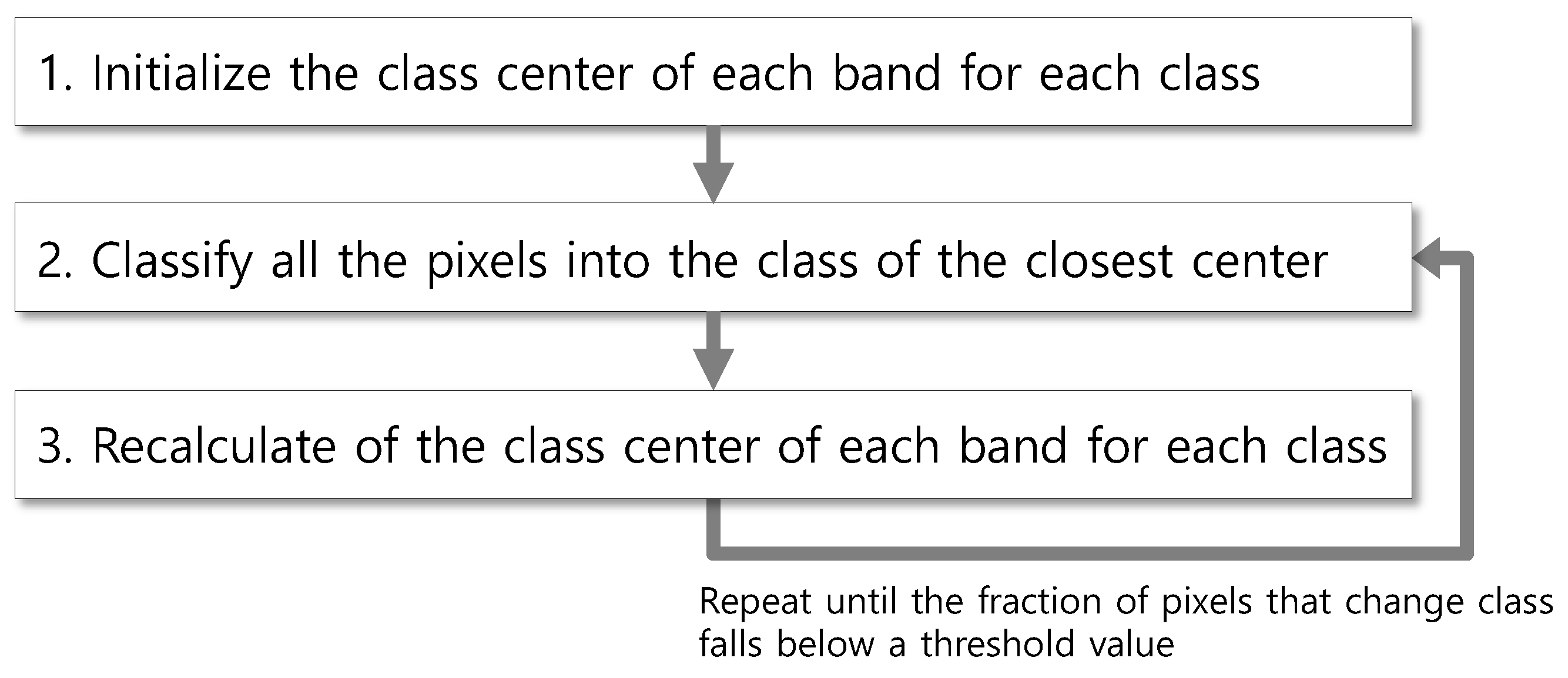
The native k-means clustering algorithm (hereafter, kMC) segments points in N dimensions into k clusters so the within-cluster sum of squares of distances is minimized [31]. The k-means clustering algorithm, applied to the unsupervised classification of a satellite image, consists of the following steps in Figure 1:
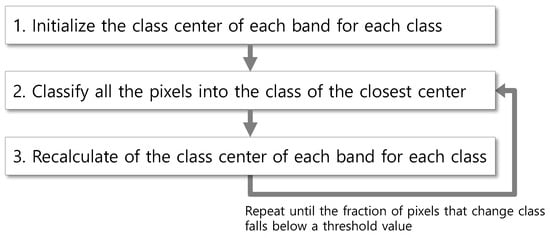
Figure 1.
A general workflow of kMC.
In step 1, various kinds of methods have been developed to produce more accurate and unbiased centers and less iterations. Among these methods, a simple furthest-point heuristic can reduce the clustering error [32]. The method first sets a random center and then adds new centers using further points from newly-retrieved points. Therefore, if the computational cost of retrieving points is not that large, it is better to sweep all points and set class centers using the statistics of member points. Simply, the difference between the pixels’ maximum and minimum values in each band is split into k segments, and the center of each segment is set as the initial center of the class (Algorithm 1).
| Algorithm 1 Pseudocode for class initialization of kMC |
|
In step 2, Euclidean distances are calculated from each point to all the class centers, and a point is assigned to the closest class. In step 3, the average value is calculated for each band of each class and is set to a new class center (Algorithm 1). Equation (1) identifies the class into which a pixel P will be classified in a multispectral satellite image composed of N bands:
where argminj(dist(P, j)) stands for the class j that minimizes the argument dist(P, j), which denotes the distance from a pixel to each class center; denotes the pixel value of band b of the pixel P; and denotes the center of band b of class j.
The pseudocode for steps 2 to 3 consists of four for-loops (Algorithm 2). The first for-loop iterates the entire classification process. The second for-loop retrieves all pixels. The third for-loop retrieves all classes, and the fourth for-loop does so for all the bands.
| Algorithm 2 Pseudocode for main classification routine of kMC |
|
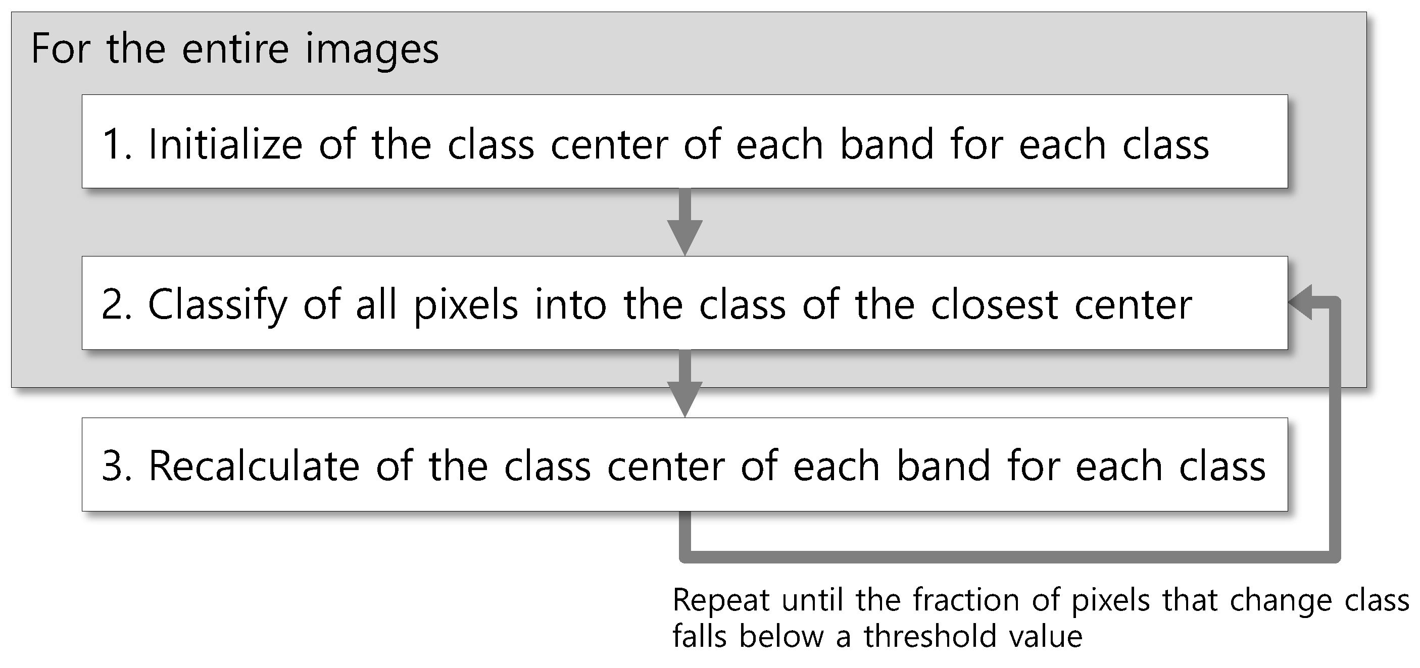
When k-means clustering is applied to multiple images, each image attains a different constitution of class signatures. Class ID is determined by chance, and an identical class ID among images does not indicate their land cover is the same. Unless it is necessary to attain separate class signatures for each image, integrated clustering of all images is the better choice for figuring out the landcover characteristics and their pixel value distribution through the entire images. In other words, if clustering is applied to continuously acquired images, it is better for a class ID to denote the same land cover through the images. In this study, a revised version of kMC is proposed, which is defined as inter-image k-means clustering (hereafter, IIkMC), to segment entire images using a single set of class signatures (Figure 2).
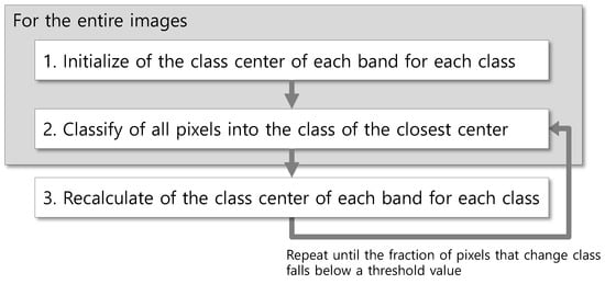
Figure 2.
A workflow of IIkMC.
The pseudocode for IIkMC introduces an additional for-loop compared to the native code (Algorithm 3). The number of bands (nBand) is assumed to be the same because the same sensor is used. However, the dimension of an image (nRow and nColumn) is specified separately for each image as the effect of resampling in geo-rectification. All images are processed using a single set of (initial) class centers, which is updated using all the pixels of entire images through the classification process. In Algorithm 3, red text indicates changes from the native code, and blue text indicates variables that calculate a single set of class signatures.
As the revised algorithm includes five for-loops, time spent increases exponentially as the size of the image, the number of classes, and the number of images increase, necessitating the improvement of processing speed. Especially, as the third for-loop takes the longest iteration, it becomes the main target to be divided and processed concurrently.
| Algorithm 3 Pseudocode for main classification routine of IIkMC |
|
Likewise, all pixels of all images should be swept when determining the initial class centers, which is the first step in Figure 1. The corresponding pseudocode is shown in Algorithm 4.
| Algorithm 4 Pseudocode for class initialization of IIkMC |
|
2.2. Parallel Processing of Inter-Image k-Means Clustering Algorithm
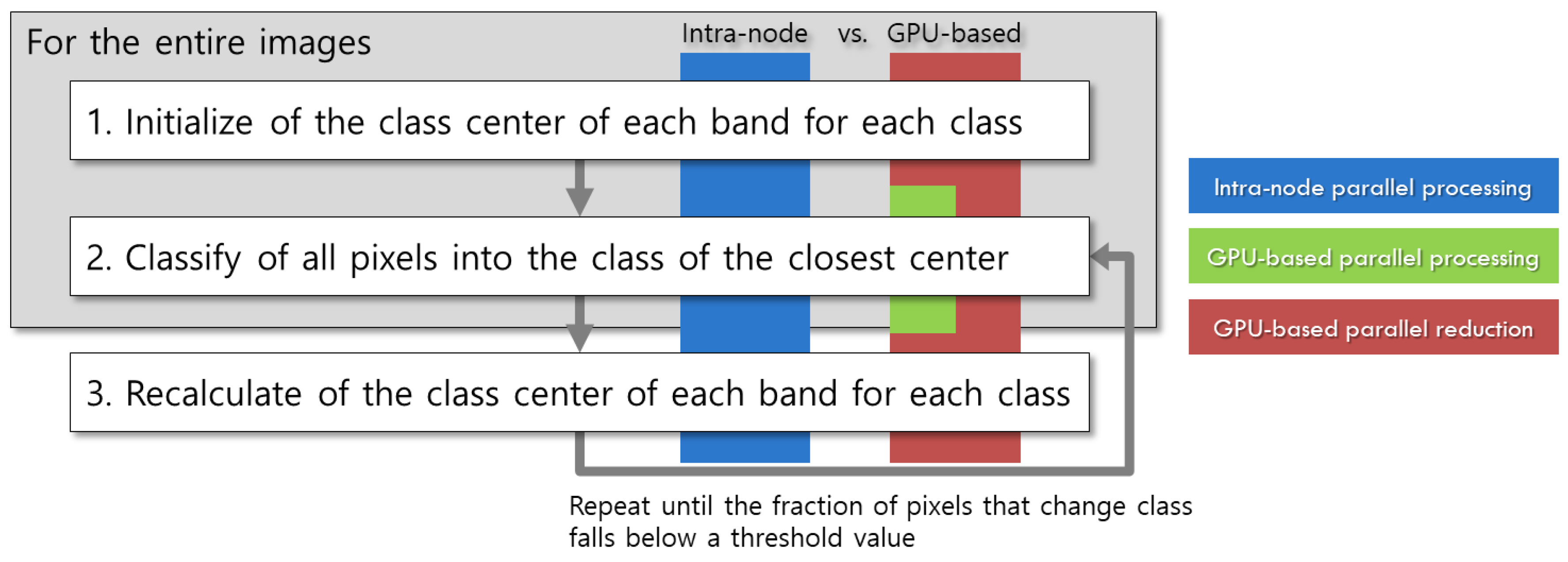
Parallel processing of kMC can be divided into intra-node parallel processing and inter-node parallel processing [33]. Intra-node parallel processing uses the multiple cores of a CPU and shared memory in a PC. OpenMP [34] programming can be used to control the multiple cores of a CPU, which all share data in the random access memory (RAM) and hard disk drive (HDD). Intra-node parallel processing can be favorably applied to the parallelization of the second loop (line 2) in Algorithm 2 because the loops constitute the worst bottleneck encountered throughout the procedures. Inter-node parallel processing uses multiple CPUs, each of which has its own OS and memory. MPI [35] programming is typically used to control CPUs in the nodes (PCs or workstations), transmitting data between the nodes through an external network (such as Ethernet). The inter-node parallelism can be implemented in a hybrid fashion with a PC cluster used to implement the inter-node method and the multiple cores of its nodes deployed to implement the intra-node method [33]. The third approach is based on general-purpose GPU. A typical GPU-based parallel implementation for kMC was applied to the second loop (line 2) in Algorithm 2 [36], in which lots of GPU cores were exploited to enormously accelerate Euclidian distance calculation. The fourth approach introduces MapReduce programming based on a Hadoop cluster for large data processing [37]. However, MapReduce programs are known to take a considerable time to process problems requiring many iterations, while OpenMP and GPU allow higher processing speed and more flexible control than MapReduce [38]. Hence, the present study develops parallel IIkMC based on the intra-node approach and the GPU method (Figure 3).

Figure 3.
Procedures to which intra-node and GPU-based parallel processing is applicable.
2.2.1. Intra-Node Parallel Processing
Intra-node parallel processing is conducted by simultaneously processing sub-images, each times the size of an entire image, using cores in a CPU. This step is simply implemented by inserting an OpenMP clause #pragma omp parallel for before the third loop (line 3) in Algorithm 3.
Unfortunately, OpenMP is known to suffer from false sharing. If this problem is not resolved, the method consumes more time than when sequential (non-parallel) processing is used. False sharing is a phenomenon that occurs when different cores modify variables that are along the same cache line. Because the memory is forced to update to maintain cache consistency, the processing speed is greatly reduced [39]. This happens frequently when the contents of variables in a for-loop are changed almost simultaneously by different cores. To prevent false sharing, the variables with changed contents in each core must be placed in a private( ) construct, and i, j, and k should be defined as private after the parallel for clause. Variables that are placed in a private( ) construct are declared independently for each core and do not interfere with each other. A reduction( ) construct is used to sum up values without false sharing. The nChanged variable is used to count the total number of pixels with changed classes, and is defined as reduction(+:nChanged). Therefore, the false sharing problem should not occur (Algorithm 5).
| Algorithm 5 Implementation of intra-node parallel processing using OpenMP |
|
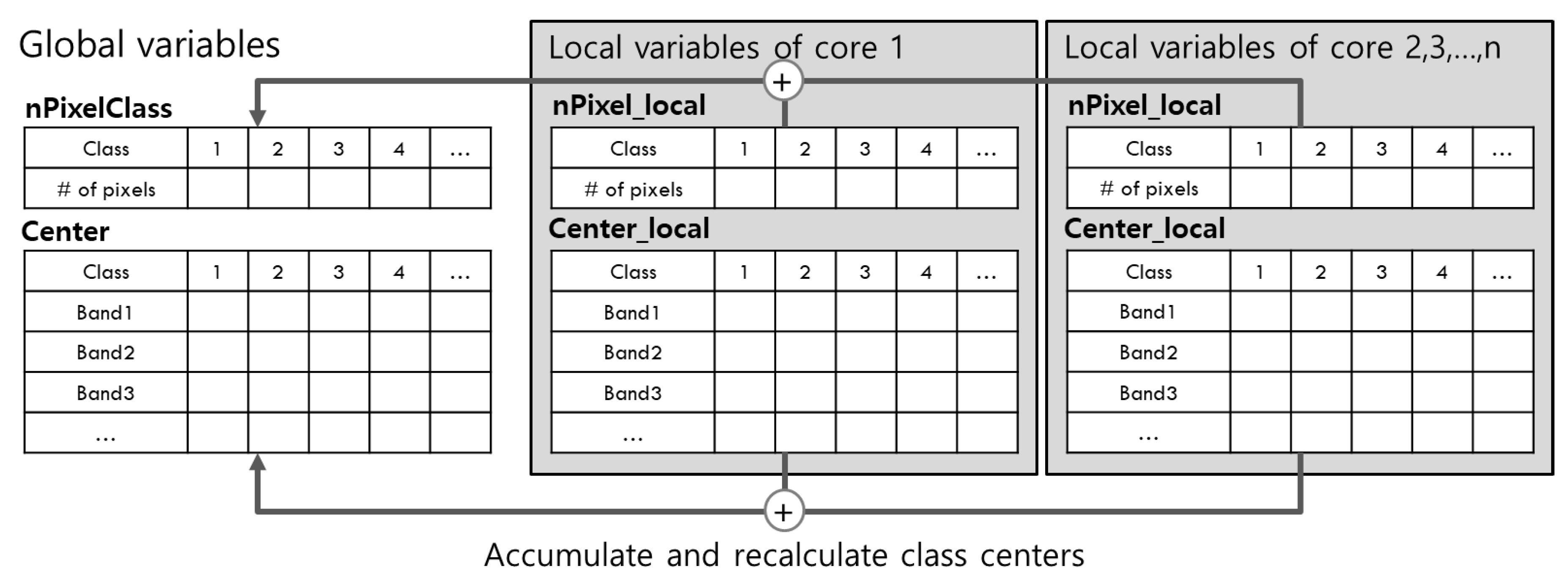
Despite these precautions, false sharing can still occur. nPixelClass and Center in Algorithm 3 are pointer arrays, which store the number of pixels classified in each class and the class center of each band. During classification, the values of nPixelClass or Center can be changed when accessed at the same time by different cores. When this happens, so does false sharing. To solve this problem, nPixelClass and Center are declared to be global variables, and nPixel_local and Center_local are declared to be local variables for each core, as illustrated in Figure 4. In each core, Center is shared during classification, but the numbers of pixels and pixel values for each class are accumulated in the local variables nPixel_local and Center_local. When classification is finished, all cores’ local variables should be summed up to the global variables Center and nPixelClass, and the centers of each class are recalculated by averaging them. This method prevents false sharing, and the pseudocode is given in Algorithm 6.
| Algorithm 6 Pseudocode for recalculation of class centers |
|

Figure 4.
Global and local declarations of variables nPixelClass and Center (revised from [33]).
As shown in Algorithm 4, when initializing the class centers as the first step in Figure 1, there is a triple for-loops, and the speed can be improved by inserting an OpenMP clause #pragma omp parallel for before the second for-loop (line 2). Since this step also causes a false sharing problem in the Min and Max variables, local variables Min_local and Max_local should be declared for each core and integrated into the global variables Min and Max. Since this is relatively simple, a more detailed explanation is omitted.
2.2.2. GPU-Based Parallel Processing
As a simple implementation method, the main classification routine (lines 2 to 7) in Algorithm 3 is divided into blocks and several blocks are concurrently processed using many arithmetic logic units (ALUs) in a GPU. In other words, a pixel of an image is assigned to an ALU, and the ALU calculates the distance to all class centers and designates the pixel to the shortest class. Thousands of ALUs concurrently conduct the same process for each pixel invoked by a kernel function. However, before the process, the class centers are initialized by a CPU and transferred to the GPU memory (hereafter, device memory), along with the image itself from main memory. The class information of each pixel, as the result of the main classification routine, is transmitted from the device memory to the main memory, and the class centers are updated by the CPU. In summary, the GPU is responsible for the distance calculation and classification of each pixel and the CPU is responsible for initializing and updating the class centers. Pseudocode for the GPU-based parallel processing is given in Algorithm 7.
| Algorithm 7 Pseudocode for GPU-based parallel processsing of IIkMC |
|
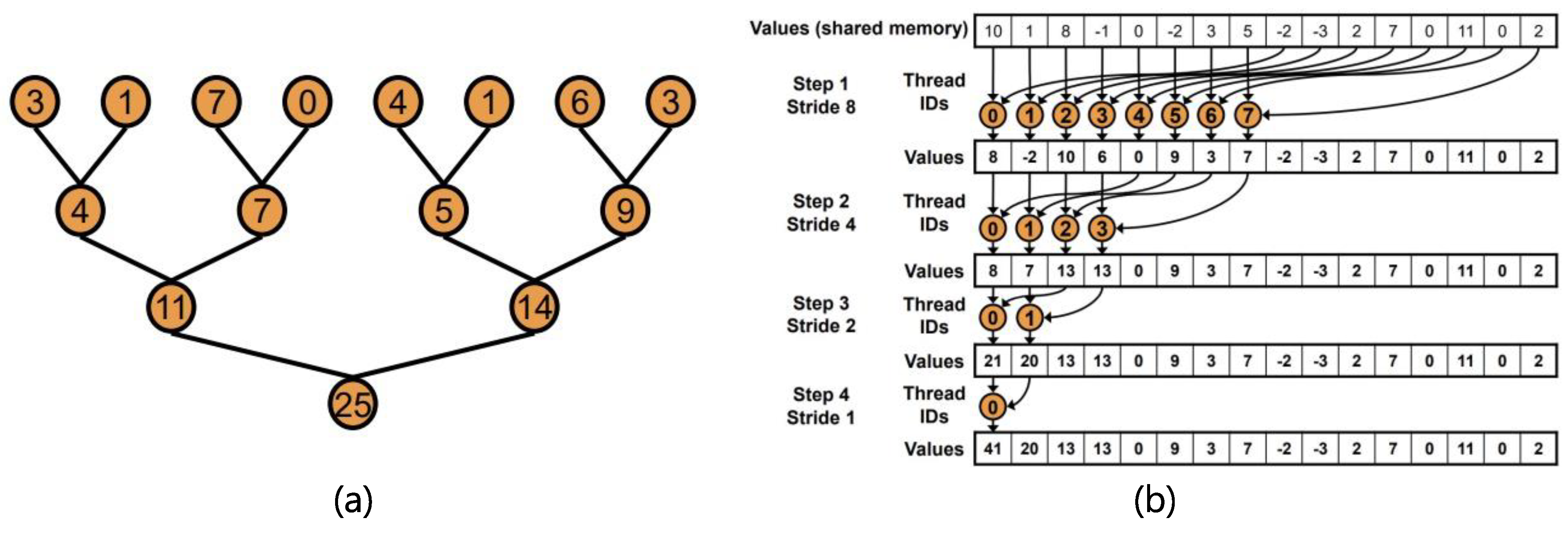
Initializing and updating class centers requires more complex designs be used for GPU-based parallel processing. Initialization requires searching the minimum and maximum values of all pixels, and updating requires summing all pixel values for each band of each class along with the counts of the pixels in each class. This kind of operation utilizes an array of numerous values to produce a single output and is referred to as “reduction”. In the intra-node parallel processing, data can be divided into several sub-sections, and each section can be serially reduced by each CPU core. Here, a serial reduction is defined to iterate through the entire array, performing the reduction on pairs of elements, and updating the accumulator until the result is obtained. However, this approach is not well suited for the massively parallel architecture of a GPU. Because each ALUs is not fast as a CPU core, it should be applied to finer pieces of tasks. Thus, a parallel reduction is conducted in the fashion that each ALU performs a summation or logical operation for finer entities. This procedure is iteratively performed for the results until a single result is derived. However, as the iteration goes on, the number of ALUs participating in the operation decreases exponentially. It is important to make as many ALUs still participate in the reduction. Parallel reduction has been sufficiently studied to enhance procedural efficiency based on CUDA [40]. In this study, sequential addressing, a middle-optimized parallel reduction among the relevant approaches (Figure 5), was applied to the following procedures in Figure 6.

Figure 5.
Illustration of parallel reduction: (a) basic concept, (b) sequential addressing [40].

Figure 6.
Procedures to which parallel reduction is applicable.
Procedure 1 is implemented in initializing class centers, procedures 2 and 3 are applied to the main classification routine, and procedure 4 is used to update the class centers. Each step is executed with a pair of a kernel invocation function and a reduction function. The kernel invocation function organizes input data into an array compatible to parallel reduction and performs the first reduction. The reduction function iterates until a result is derived using a parallel reduction routine. In this way, IIkMC is fully parallelized using a GPU without any CPU implementations. The pseudocode is shown in Algorithm 8. Unlike line 7 in Algorithm 7, one more argument is given within <<< >>> in the kernel invocation in Algorithm 8. This dramatically improves the speed of the parallel reduction using cache memory (shared memory in CUDA) allocated to each ALU. However, the details of this are omitted in the manuscript.
| Algorithm 8 Pseudocode for fully parallelized GPU-based IIkMC using parallel reduction |
//Class center initialization
|
3. Evaluation and Discussions
3.1. Evaluation Method
A series of adjacent PlanetScope images were processed using kMC and IIkMC, and the classification results were compared. IIkMC was implemented in a sequential code (without parallel processing), an intra-node parallel code, a GPU-based parallel code, and a GPU-based parallel code using the parallel reduction. The performance of the parallel codes was compared to the sequential variant.
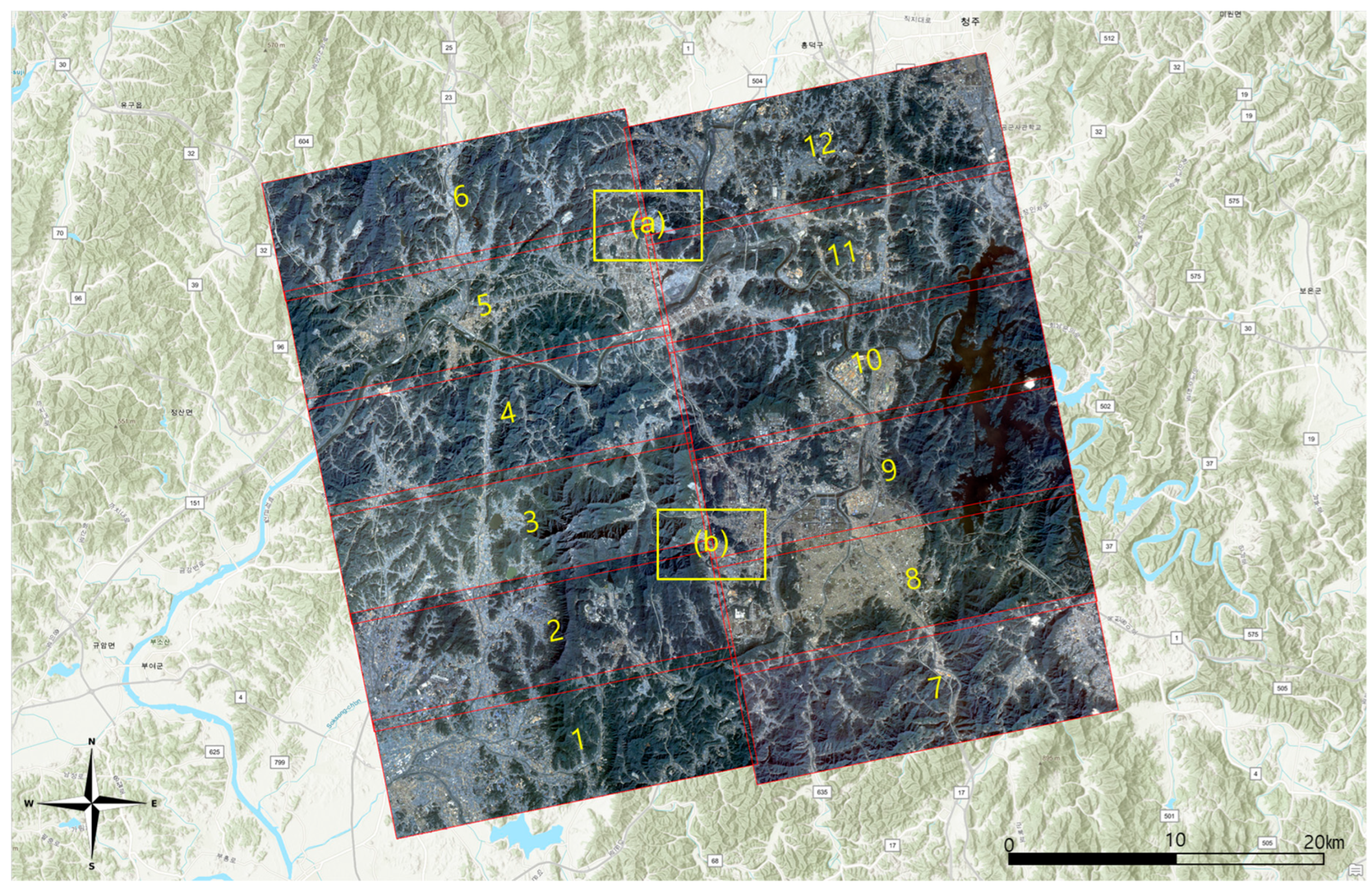
A total of twelve images were achieved over two days from 30 October 2018 to 31 October 2018 (Figure 7). Each image is composed of four multi-spectral bands (red, green, blue, and infra-red) and the file type is 16-bit geotiff. The dimension of each image is approximately 8.2 k × 3.9 k and the average size in the uncompressed tiff is 244 MB. The computing system has an AMD Ryzen 9 CPU consisting of 16 cores for intra-node parallel processing and an NVIDIA RTX 3090 Ti graphics card for GPU-based parallel processing (Table 1). The number of classes (k) is eight, and the iteration termination condition is 1.0% (Table 2).

Figure 7.
Placement of 12 PlanetScope images (Enlargements of (a) and (b) are in Appendix A, and location names are in local terms.)

Table 1.
Specifications of the computing system.

Table 2.
Parameters of k-means clustering.
3.2. Evaluation of Clustering Results
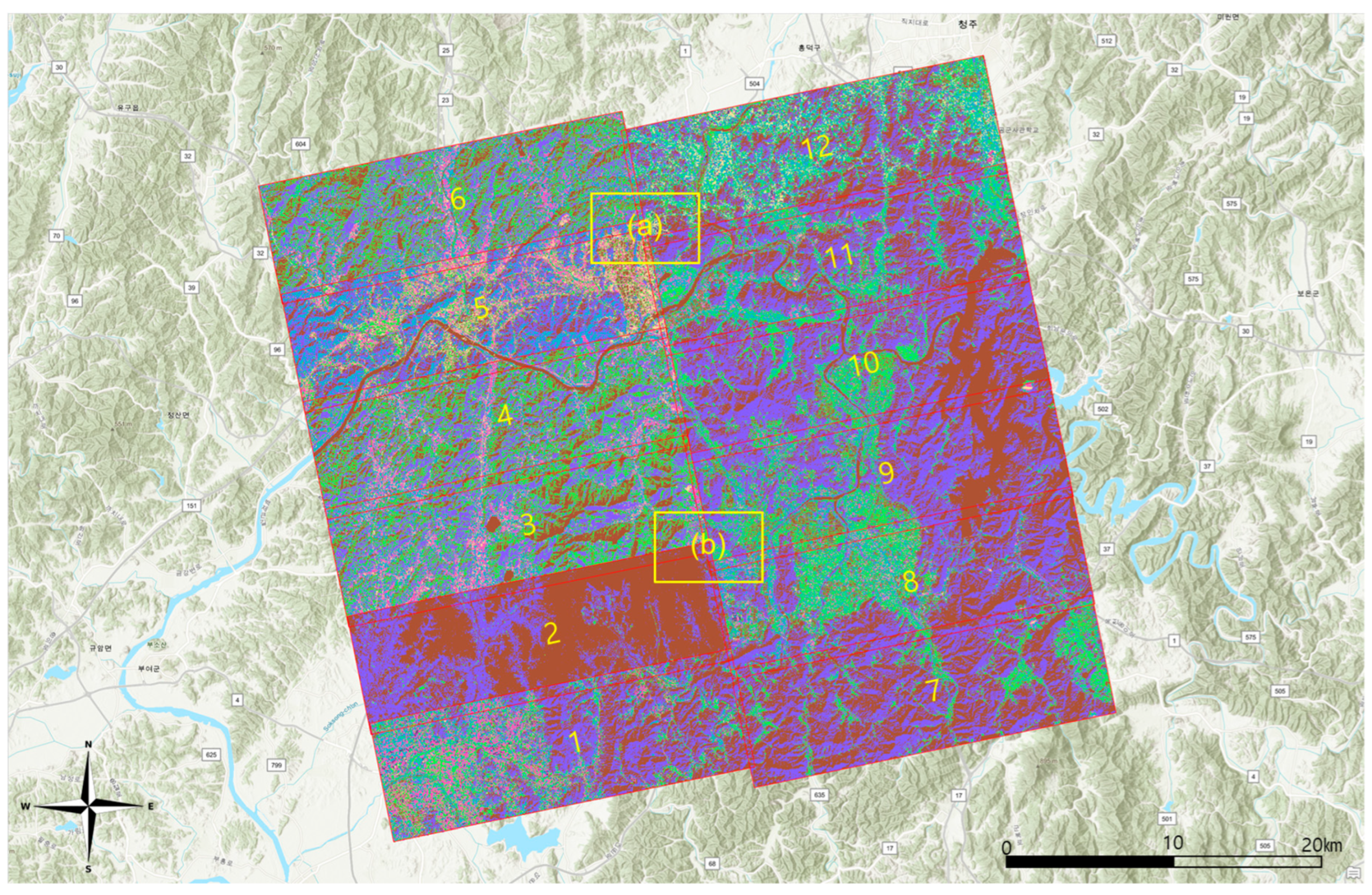
The results of the separate processing of each image using kMC are shown in Table 3 and Figure 8. A same-color map was applied to each result to match the same class ID with the same color. The number of iterations differed greatly, and image 3 was processed after three iterations, resulting in incomplete segmentation. With smaller termination condition, it would have produced different results, but it should be remarked 1.0% was not an unreasonable condition. One class was canceled in image 9, and two classes were canceled in image 11, which may have occurred accidentally due to the spectral characteristics of the initial and updated class centers. This problem might be solved by applying class-splitting step to the classification routine, which was not considered in this study. Results 1 and 7 to 12 appear to have similar class signatures compatible among themselves; images 3, 4, and 6 also might, but the rest do not.

Table 3.
Results of kMC (The numbers next to each class IDs are the numbers of entities and ratios of the pixels classified to the classes.).
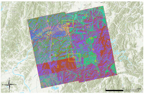
Figure 8.
Results of kMC (Enlargements of (a) and (b) are in Appendix A, and location names are in local terms.)
The result of concurrently processing the 12 images using IIkMC is shown in Table 4 and Figure 9. The result was derived after 55 iterations, and the class signatures appeared to be compatible throughout the results. From the enlarged image of Figure 7 (a) in Figure A1 and the corresponding results in Figure A2 and Figure A3, it can be clearly seen IIkMC has better class compatibility among the results. From the enlarged image of Figure 7 (b) in Figure A4 and the corresponding results in Figure A5 and Figure A6, it could be confirmed a complete result was obtained for image 2, which was not properly segmented by kMC. From the inspection, it was also confirmed none of the classes were canceled in the results of images 9 and 11.

Table 4.
Results of IIkMC.
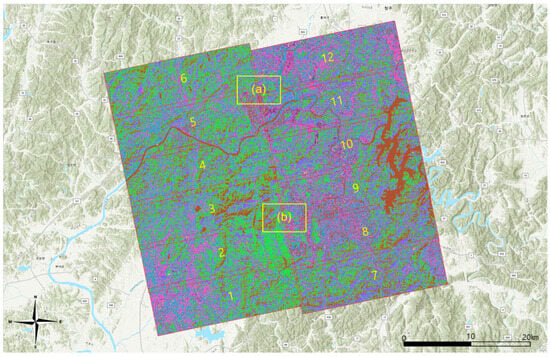
Figure 9.
Results of IIkMC (Enlargements of (a) and (b) are in Appendix A, and location names are in local terms.)
However, from Figure A3 and Figure A6, it could be remarked over-segmentation might have occurred in the results of IIkMC. The possible reason for this was acceptance of the spectral features from multiple images could have broadened the spectral distribution, and, as a result, separability among classes may have decreased. Separability can be better understood by inspecting the distribution of the center and standard deviation of each class in the spectral domain. In the results of kMC, the standard deviation starts in the mid 100 s (Table A1), while in IIkMC, it starts in the late 200 s (Table A2). A larger standard deviation can imply lower separability. Therefore, it will be necessary to reduce the spectral distribution by applying histogram matching among images before clustering.
Nevertheless, the standard deviation of kMC is very different for each image and band, and the large values exceed 3000. This is compared to the standard deviation of IIkMC, which does not exceed the early 2000 s. Therefore, it can be confirmed the result of IIkMC is more stable than that of kMC, even from the view of separability. Moreover, since it is challenging to identify a set of representative class signatures from KMC (i.e., widely distributed class centers and standard deviation among images), IIkMC is considered a better solution.
3.3. Evaluation of Parallel Processing Performance
Parallel processing performance is typically evaluated using two indices, efficiency and speedup, both of which are defined in terms of the processing time versus the number of cores or computing nodes involved (Equation (2)). In the ideal case, speedup is the same as the number of cores or computing nodes, and efficiency should be 1.0. This indicates the increase in execution speed is exactly proportional to the number of cores or computing nodes involved. However, according to Amdahl’s law [41], this is not achievable in reality. Reasons for this include unequal workload among cores and nodes, as well as unparallelizable procedures. In addition, in some cases, the efficiency might exceed 1.0; this is called super-linearity. This can occur when processing an exceptional amount of data or when the complexity is beyond the ability of a single core or node [42]. Speedup and efficiency are defined as:
where p is the number of cores (or computing nodes) and and denote the execution times for sequential and parallel processing, respectively.
The execution times were measured for the sequential code, the intra-node code, the GPU-based code, and the GPU-based code with parallel reduction for IIkMC. To calculate the speedup and the efficiency of the intra-node code, was set as the execution time of the sequential code, and was set as that of the intra-node code using all cores. However, since it is ambiguous to define p for the GPU-based code, the efficiency is not presented (Table 5).

Table 5.
Execution time, speedup, and efficiency of parallel IIkMC.
The results are listed in Table 5. Processing with sequential code was very burdensome and required 5765.18 s (=1.6 h) to process 12 images (=2.86 GB). On the contrary, the intra-node code took 449.27 s (=7.5 min). This is about 13 times faster, meaning the task can be finished within an acceptable time. The GPU-based code processed the data 25.53 times faster than sequential code and 2.00 times faster than intra-node code. Furthermore, the GPU-based code with parallel reduction processed 1.53 times faster than the GPU-based code. In this study, sequential addressing, a middle-optimized parallel reduction approach, was applied. With more optimized reduction approaches, the processing speed will be further improved. Additionally, it can be predicted the speed can be maximized by using multi-GPUs.
Finally, this study verified whether the results obtained using the sequential, intra-node, and GPU-based codes with and without parallel reduction, matched. The class centers of each band and the classified number of pixels of the results were compared. No discrepancy was detected among the results, confirming they matched completely.
3.4. Discussion
Applying kMC and IIkMC to 12 planetscope images revealed quite different results. In the results of kMC, using 12 consecutively acquired images that might constitute similar land cover, the number of iterations was significantly different, some images were not clustered appropriately, and some classes were canceled during iteration. Class signatures of kMC proved challenging because choosing a representative one among images would take a lot of work. On the other hand, IIkMC conducted stable clustering while assigning consistent classes to all the images. Although the standard deviations were estimated to be slightly larger, the results were expected to provide a comprehensive result by delivering a single set of class signatures for all images.
Because of its efficiency, kMC is still widely used for unsupervised classification of satellite images. Nevertheless, as the capacity or quantity of images increases, the processing time of IIkMC increases exponentially. The intra-node parallel processing and GPU-based parallel processing succeeded in increasing the speed of IIkMC several times faster than sequential processing. In addition, the performance is further improved with the introduction of parallel reduction and is expected to be enhanced by optimizing parallel reduction and utilizing multi-GPU. Therefore, it will be possible to process data acquired in a more extensive range of areas, including satellite and drone images ranging from hundreds to thousands.
4. Conclusions
In this study, IIkMC was introduced for the unsupervised classification of satellite images acquired in series. The results can be summarized in three points as follows:
- -
- derived a single set of class signatures for multiple satellite images;
- -
- performed complete classification of all images, granting consistent class IDs;
- -
- implemented intra-node and GPU-base parallel processing.
A single set of class signatures was derived, and each image was consistently classified so the classification results were compatible between the images. In addition, some images were completely processed could not be correctly segmented by kMC. However, IIkMC also revealed the possibility the separability among classes could be weakened because wider spectral features from multiple images were merged into each class. Nevertheless, it should be remarked IIkMC provides more reliable results, potentially facilitating overall inspection of multiple images and training data generation for supervised classification or deep learning.
kMC is a computationally intensive algorithm, making it burdensome to apply to large images, which is also the case for IIkMC. With the parallelized IIkMC using multi-cores of a CPU and a GPU, the processing speed could be dramatically improved. Thus, large volumes of satellite images acquired from an extensive range of areas are expected to be plausibly inspected prior to intensive analysis or supervised classification.
For better performance of IIkMC, future works aim to improve the class center management and enhance class separability. The former includes class center initialization along with class separation and integration based on data characteristics, similar to ISODATA clustering. The latter will be achieved by normalizing the radiometric distributions among images. GPU-based approaches will be improved by implementing further optimized parallel reduction, manipulating high-performance operations introduced in cuBLAS [43], and modifying parallel code to fit using multi-GPUs.
Author Contributions
Conceptualization, S.H.; methodology, S.H.; software, S.H.; data curation, J.L.; writing—original draft preparation, S.H.; supervision, S.H.; project administration, J.L. All authors have read and agreed to the published version of the manuscript.
Funding
This research was supported by the consigned research project funded by Korea Aerospace Research Institute, grant number FR22H00W02.
Data Availability Statement
No new data were created or analyzed in this study. Data sharing is not applicable to this article.
Conflicts of Interest
The authors declare no conflicts of interest.
Appendix A

Table A1.
Class centers and standard deviations produced by kMC.
Table A1.
Class centers and standard deviations produced by kMC.
| Image ID | 1 | 2 | 3 | 4 | 5 | 6 | ||||||
| Center | Std. dev. | Center | Std. dev. | Center | Std. dev. | Center | Std. dev. | Center | Std. dev. | Center | Std. dev. | |
| Class 1 | ||||||||||||
| Band 1 | 3281 | 198 | 3453 | 252 | 3151 | 171 | 3229 | 167 | 3357 | 212 | 3241 | 152 |
| Band 2 | 2697 | 210 | 2931 | 285 | 2535 | 195 | 2617 | 186 | 2744 | 229 | 2636 | 166 |
| Band 3 | 1921 | 230 | 2193 | 338 | 1752 | 197 | 1812 | 203 | 1919 | 239 | 1851 | 194 |
| Band 4 | 2862 | 599 | 3812 | 899 | 2325 | 499 | 2412 | 504 | 2337 | 520 | 2608 | 467 |
| Class 2 | ||||||||||||
| Band 1 | 3494 | 183 | 4561 | 475 | 3495 | 167 | 3525 | 165 | 3424 | 145 | 3538 | 168 |
| Band 2 | 3019 | 205 | 4164 | 442 | 3050 | 185 | 3088 | 187 | 2892 | 163 | 3091 | 195 |
| Band 3 | 2301 | 244 | 3636 | 524 | 2366 | 245 | 2401 | 245 | 2129 | 203 | 2417 | 264 |
| Band 4 | 4544 | 595 | 4364 | 759 | 5048 | 499 | 5070 | 491 | 3810 | 387 | 5022 | 450 |
| Class 3 | ||||||||||||
| Band 1 | 4156 | 306 | 6701 | 821 | 3350 | 137 | 3364 | 125 | 4091 | 263 | 3394 | 131 |
| Band 2 | 3656 | 278 | 6215 | 758 | 2822 | 147 | 2835 | 139 | 3594 | 239 | 2869 | 143 |
| Band 3 | 2989 | 305 | 5513 | 824 | 2095 | 195 | 2091 | 184 | 2902 | 255 | 2139 | 193 |
| Band 4 | 3455 | 396 | 4894 | 740 | 3740 | 398 | 3775 | 386 | 3357 | 475 | 3859 | 356 |
| Class 4 | ||||||||||||
| Band 1 | 4326 | 224 | 10,072 | 1130 | 4053 | 253 | 3980 | 217 | 3616 | 203 | 4066 | 243 |
| Band 2 | 3961 | 224 | 9576 | 979 | 3590 | 234 | 3509 | 205 | 3175 | 230 | 3607 | 227 |
| Band 3 | 3462 | 314 | 8808 | 1018 | 2963 | 265 | 2874 | 248 | 2466 | 280 | 2996 | 270 |
| Band 4 | 4494 | 502 | 7198 | 1432 | 3798 | 487 | 3659 | 461 | 5024 | 501 | 3758 | 482 |
| Class 5 | ||||||||||||
| Band 1 | 5061 | 331 | 13,581 | 1378 | 4602 | 313 | 4467 | 267 | 4512 | 285 | 4638 | 324 |
| Band 2 | 4619 | 246 | 12,970 | 941 | 4215 | 245 | 4065 | 222 | 4097 | 241 | 4261 | 265 |
| Band 3 | 4065 | 369 | 12,892 | 1184 | 3701 | 301 | 3539 | 278 | 3528 | 289 | 3780 | 329 |
| Band 4 | 4162 | 550 | 11,029 | 2099 | 4383 | 567 | 4203 | 493 | 4100 | 516 | 4361 | 532 |
| Class 6 | ||||||||||||
| Band 1 | 8127 | 842 | 17,241 | 1815 | 5503 | 464 | 5291 | 373 | 5359 | 365 | 5694 | 517 |
| Band 2 | 7597 | 750 | 14,967 | 828 | 5046 | 342 | 4833 | 284 | 4907 | 296 | 5238 | 406 |
| Band 3 | 6754 | 842 | 16,878 | 1484 | 4466 | 416 | 4232 | 367 | 4288 | 370 | 4632 | 475 |
| Band 4 | 5764 | 1043 | 13,809 | 2638 | 4428 | 618 | 4158 | 567 | 4030 | 593 | 4409 | 607 |
| Class 7 | ||||||||||||
| Band 1 | 6150 | 580 | 20,635 | 1493 | 7465 | 840 | 8833 | 1262 | 6655 | 641 | 7863 | 1024 |
| Band 2 | 5606 | 428 | 15,570 | 1058 | 6913 | 749 | 8261 | 1068 | 6196 | 569 | 7289 | 943 |
| Band 3 | 4858 | 520 | 19,338 | 1590 | 6159 | 824 | 7424 | 1098 | 5537 | 637 | 6474 | 1045 |
| Band 4 | 4525 | 616 | 18,004 | 1866 | 5385 | 923 | 5477 | 761 | 4530 | 582 | 5179 | 805 |
| Class 8 | ||||||||||||
| Band 1 | 11,536 | 1969 | 19,443 | 2192 | 11,215 | 1650 | 6590 | 570 | 10,538 | 1946 | 15,141 | 3121 |
| Band 2 | 11,066 | 1517 | 14,170 | 1030 | 10,759 | 1404 | 6077 | 478 | 9924 | 1753 | 12,943 | 1219 |
| Band 3 | 10,633 | 2014 | 18,900 | 1635 | 10,407 | 1773 | 5355 | 609 | 9275 | 2128 | 13,824 | 3245 |
| Band 4 | 9115 | 1938 | 26,417 | 2234 | 9123 | 1895 | 4585 | 567 | 6666 | 1819 | 10,612 | 2478 |
| Image ID | 7 | 8 | 9 | 10 | 11 | 12 | ||||||
| Center | Std. dev. | Center | Std. dev. | Center | Std. dev. | Center | Std. dev. | Center | Std. dev. | Center | Std. dev. | |
| Class 1 | ||||||||||||
| Band 1 | 3826 | 191 | 3862 | 219 | 3887 | 210 | 3870 | 235 | 3955 | 198 | 4031 | 197 |
| Band 2 | 3063 | 214 | 3079 | 225 | 3093 | 225 | 3063 | 246 | 3191 | 214 | 3283 | 207 |
| Band 3 | 2114 | 246 | 2074 | 223 | 2064 | 242 | 2016 | 248 | 2186 | 244 | 2288 | 230 |
| Band 4 | 2835 | 617 | 2540 | 657 | 2365 | 746 | 2147 | 691 | 2736 | 699 | 2994 | 612 |
| Class 2 | ||||||||||||
| Band 1 | 4079 | 191 | 4122 | 244 | 4108 | 214 | 4086 | 241 | 4155 | 195 | 4256 | 230 |
| Band 2 | 3453 | 214 | 3480 | 267 | 3460 | 243 | 3428 | 278 | 3519 | 224 | 3627 | 258 |
| Band 3 | 2607 | 271 | 2592 | 314 | 2543 | 288 | 2500 | 328 | 2584 | 267 | 2698 | 308 |
| Band 4 | 4747 | 690 | 4574 | 688 | 4528 | 749 | 4453 | 737 | 4664 | 659 | 4765 | 618 |
| Class 3 | ||||||||||||
| Band 1 | 4975 | 385 | 4867 | 312 | 5179 | 417 | 5050 | 364 | 4794 | 276 | 4686 | 257 |
| Band 2 | 4313 | 355 | 4137 | 294 | 4533 | 375 | 4348 | 339 | 4161 | 272 | 4021 | 239 |
| Band 3 | 3456 | 387 | 3075 | 291 | 3658 | 422 | 3359 | 358 | 3333 | 320 | 3148 | 266 |
| Band 4 | 3836 | 569 | 2922 | 479 | 3865 | 704 | 3350 | 669 | 3809 | 536 | 3552 | 453 |
| Class 4 | ||||||||||||
| Band 1 | 6335 | 601 | 5543 | 369 | 6491 | 668 | 6023 | 544 | 5585 | 357 | 5245 | 292 |
| Band 2 | 5637 | 519 | 4851 | 311 | 5840 | 533 | 5340 | 448 | 5011 | 296 | 4644 | 233 |
| Band 3 | 4746 | 579 | 3886 | 327 | 4925 | 644 | 4395 | 461 | 4292 | 361 | 3873 | 273 |
| Band 4 | 4436 | 650 | 3676 | 620 | 4427 | 676 | 4091 | 734 | 4188 | 571 | 4057 | 518 |
| Class 5 | ||||||||||||
| Band 1 | 8772 | 941 | 6590 | 515 | 9018 | 1164 | 8044 | 895 | 6713 | 594 | 9691 | 1210 |
| Band 2 | 8017 | 822 | 5861 | 403 | 8272 | 955 | 7342 | 801 | 6122 | 478 | 9001 | 1096 |
| Band 3 | 6960 | 811 | 4887 | 483 | 7086 | 1013 | 6376 | 900 | 5376 | 569 | 7955 | 1144 |
| Band 4 | 5742 | 988 | 4145 | 639 | 5596 | 931 | 5029 | 912 | 4559 | 591 | 6105 | 955 |
| Class 6 | ||||||||||||
| Band 1 | 12,599 | 1158 | 8187 | 796 | 14,179 | 1804 | 12,563 | 1876 | 9361 | 1489 | 5956 | 408 |
| Band 2 | 11,630 | 1069 | 7556 | 691 | 13,058 | 1597 | 11,595 | 1735 | 8693 | 1352 | 5371 | 296 |
| Band 3 | 10,148 | 1049 | 6723 | 875 | 11,505 | 1588 | 10,171 | 1635 | 7794 | 1392 | 4635 | 370 |
| Band 4 | 7064 | 1227 | 5192 | 856 | 8182 | 1518 | 7232 | 1538 | 5843 | 1136 | 4397 | 577 |
| Class 7 | ||||||||||||
| Band 1 | 19,047 | 2628 | 11,795 | 1463 | 19,464 | 2214 | 19,536 | 3024 | N/A | N/A | 7268 | 633 |
| Band 2 | 16,634 | 1030 | 11,451 | 1476 | 14,886 | 785 | 15,930 | 925 | N/A | N/A | 6634 | 503 |
| Band 3 | 16,940 | 2590 | 10,686 | 1527 | 18,196 | 1760 | 17,435 | 3092 | N/A | N/A | 5776 | 665 |
| Band 4 | 11,956 | 1760 | 7526 | 1227 | 15,681 | 3574 | 12,068 | 5175 | N/A | N/A | 4928 | 683 |
| Class 8 | ||||||||||||
| Band 1 | 22,716 | 2927 | 20,948 | 2854 | N/A | N/A | 6921 | 2375 | N/A | N/A | 20,006 | 4133 |
| Band 2 | 16,680 | 1941 | 15,563 | 1294 | N/A | N/A | 6438 | 2466 | N/A | N/A | 14,954 | 1298 |
| Band 3 | 20,584 | 2917 | 19,057 | 2716 | N/A | N/A | 5441 | 3098 | N/A | N/A | 17,699 | 3775 |
| Band 4 | 5940 | 1393 | 16,343 | 6137 | N/A | N/A | 22,647 | 6216 | N/A | N/A | 8690 | 6287 |

Table A2.
Class centers and standard deviations produced by IIkMC.
Table A2.
Class centers and standard deviations produced by IIkMC.
| Class 1 | Class 2 | Class 3 | Class 4 | Class 5 | Class 6 | Class 7 | Class 8 | ||
|---|---|---|---|---|---|---|---|---|---|
| Band 1 | Center | 3571 | 3883 | 3605 | 4428 | 5082 | 7850 | 6125 | 12,043 |
| Std. dev. | 361 | 343 | 292 | 318 | 373 | 856 | 485 | 2250 | |
| Band 2 | Center | 2853 | 3365 | 3011 | 3838 | 4552 | 7227 | 5510 | 11,206 |
| Std. dev. | 296 | 306 | 230 | 262 | 277 | 733 | 371 | 1717 | |
| Band 3 | Center | 1929 | 2585 | 2196 | 3044 | 3858 | 6348 | 4688 | 10,279 |
| Std. dev. | 240 | 323 | 220 | 301 | 343 | 833 | 477 | 2171 | |
| Band 4 | Center | 2253 | 5058 | 3757 | 3553 | 4135 | 5167 | 4224 | 7644 |
| Std. dev. | 526 | 538 | 422 | 554 | 637 | 841 | 641 | 2075 |
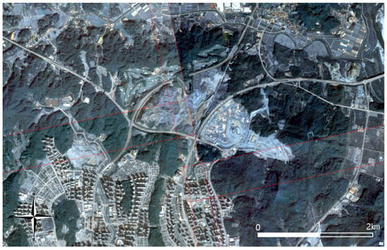
Figure A1.
Enlarged view of Figure 7 (a).
Figure A1.
Enlarged view of Figure 7 (a).
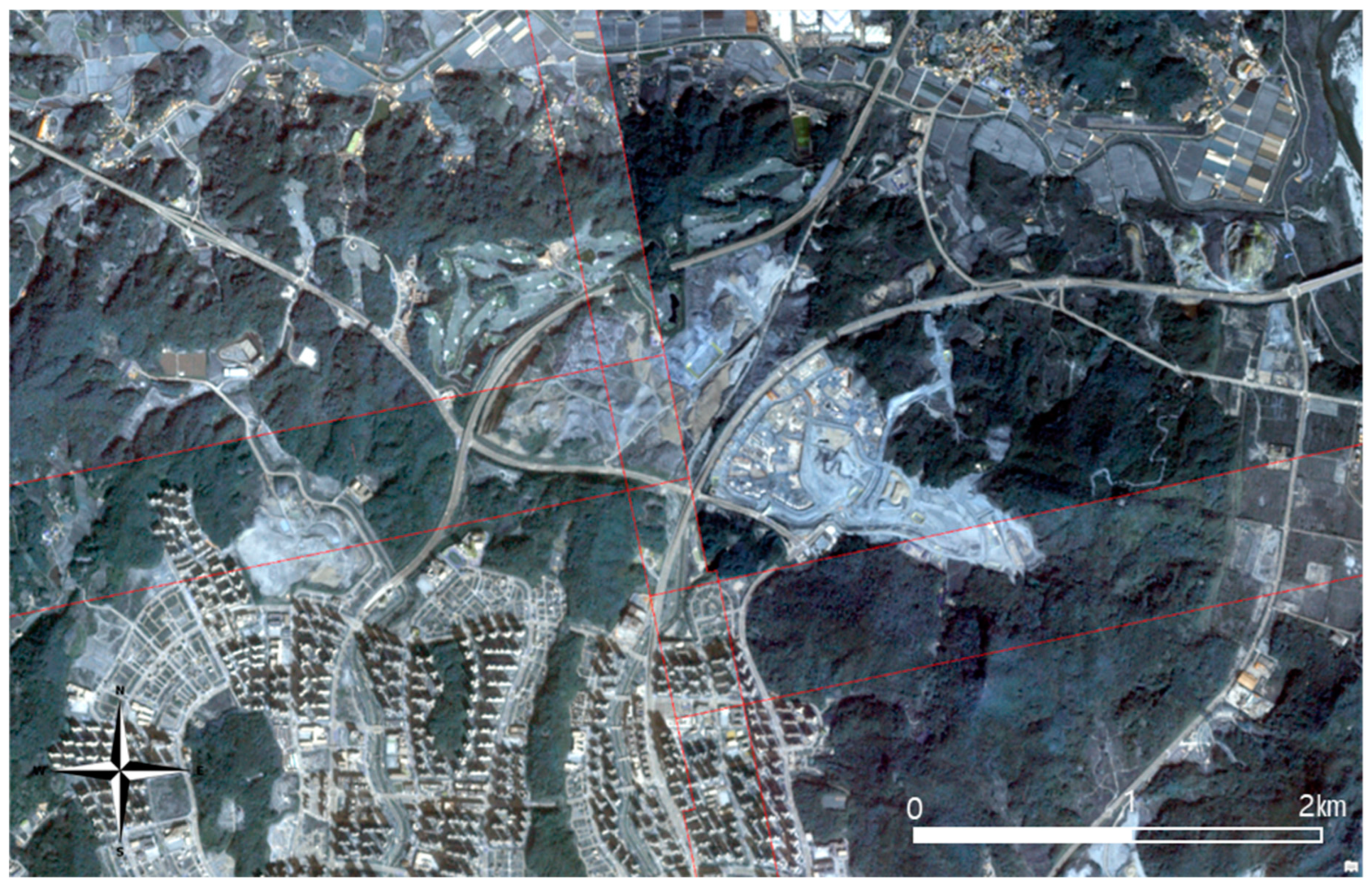
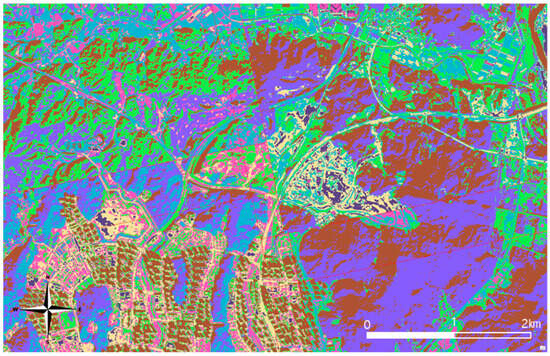
Figure A2.
Results of kMC (enlarged view of Figure 8 (a)).
Figure A2.
Results of kMC (enlarged view of Figure 8 (a)).
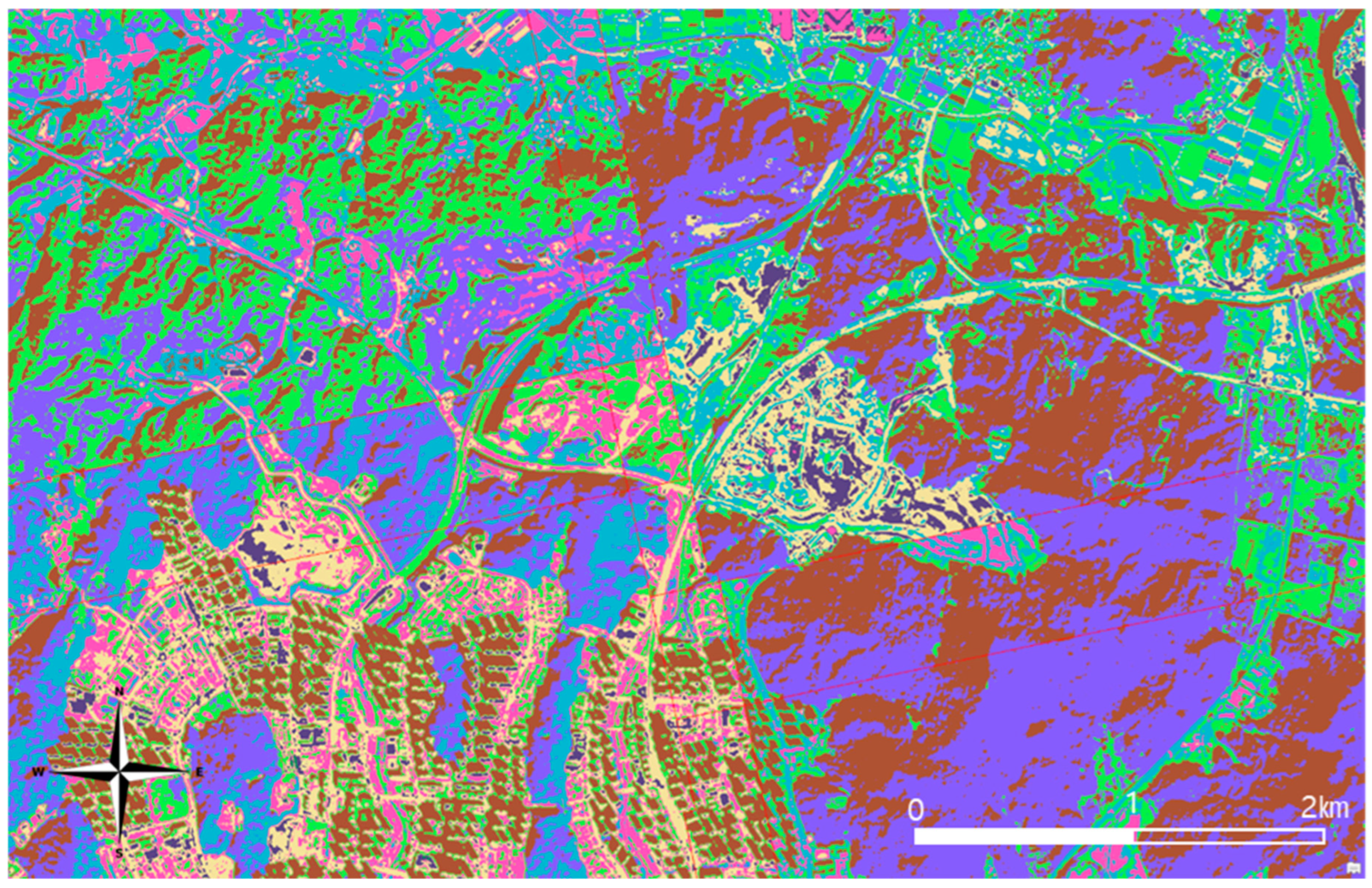
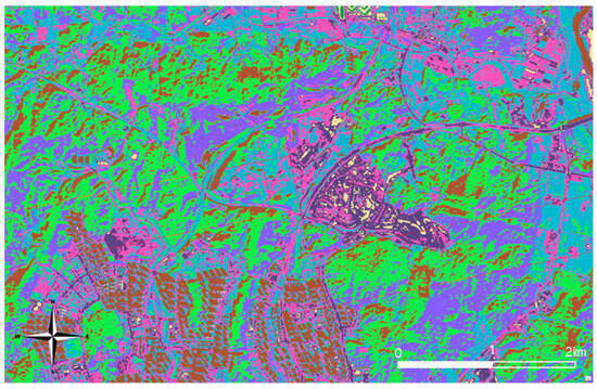
Figure A3.
Results of IIkMC (enlarged view of Figure 9 (a)).
Figure A3.
Results of IIkMC (enlarged view of Figure 9 (a)).
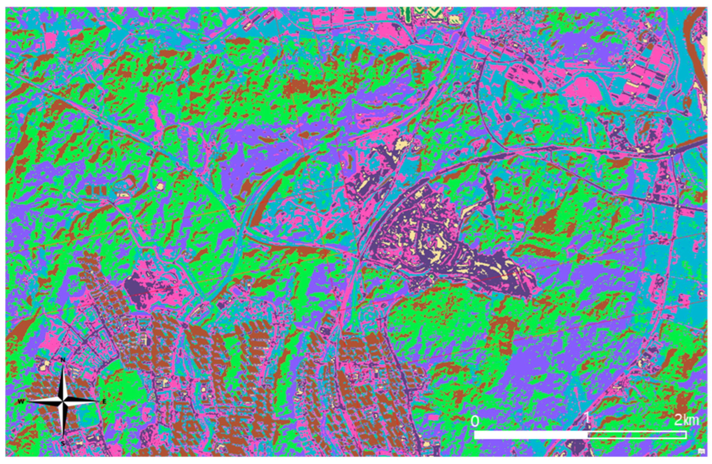
Figure A4.
Enlarged view of Figure 7 (b).
Figure A4.
Enlarged view of Figure 7 (b).
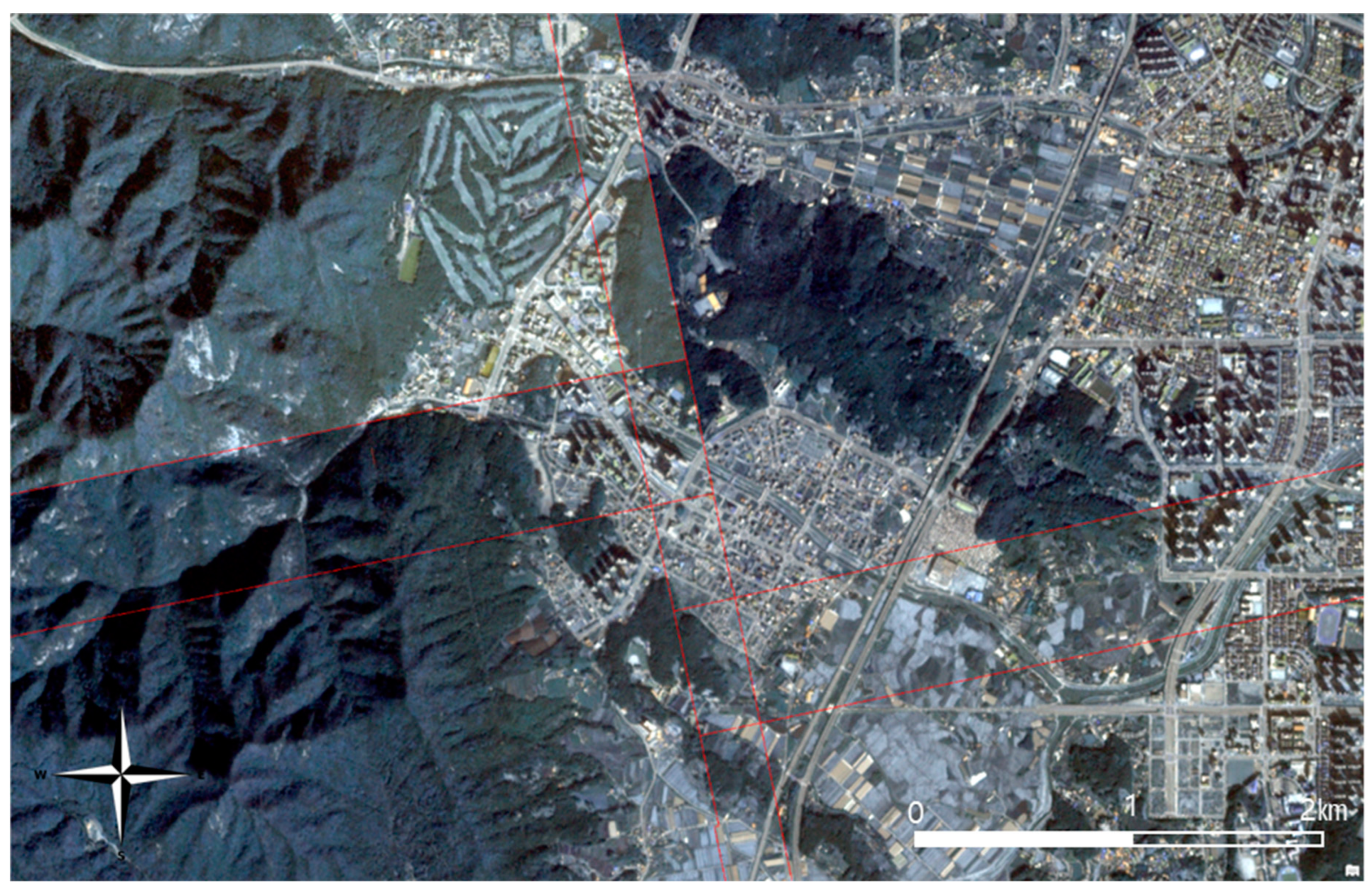

Figure A5.
Results of kMC (enlarged view of Figure 8 (b)).
Figure A5.
Results of kMC (enlarged view of Figure 8 (b)).
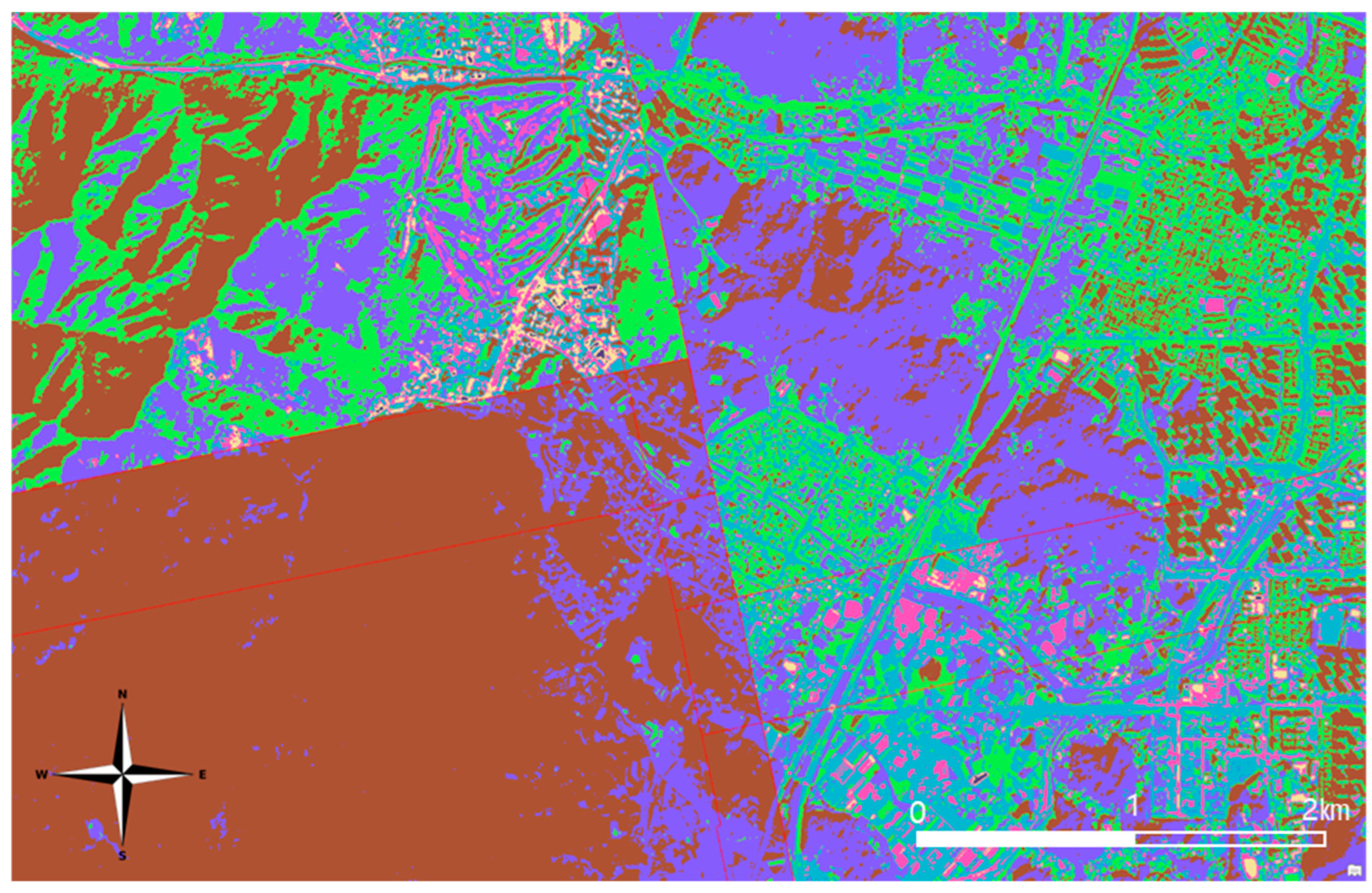
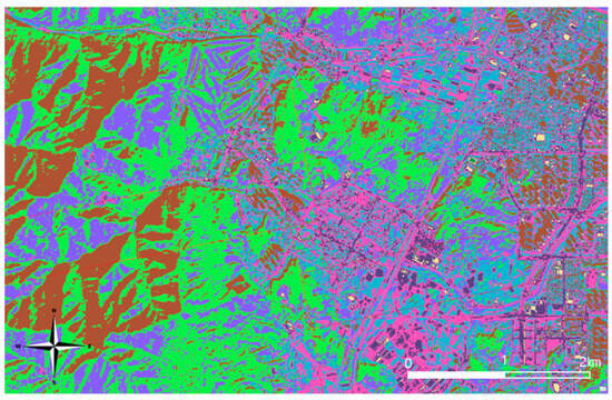
Figure A6.
Results of IIkMC (enlarged view of Figure 9 (b)).
Figure A6.
Results of IIkMC (enlarged view of Figure 9 (b)).
References
- The European Space Agency PlanetScope Overview—Earth Online. Available online: https://earth.esa.int/eogateway/missions/planetscope/description (accessed on 11 November 2023).
- Healey, R.G.; Minetar, M.J.; Dowers, S. (Eds.) Parallel Processing Algorithms for GIS; Taylor & Francis Ltd.: London, UK, 1997; ISBN 0-7484-0508-9. [Google Scholar]
- Zhao, L.; Chen, L.; Ranjan, R.; Choo, K.-K.R.; He, J. Geographical Information System Parallelization for Spatial Big Data Processing: A Review. Clust. Comput. 2016, 19, 139–152. [Google Scholar] [CrossRef]
- Plaza, A.J.; Chang, C.-I. High Performance Computing in Remote Sensing; Chapman & Hall/CRC: Boca Raton, FL, USA, 2007; ISBN 1-58488-662-5. [Google Scholar]
- Bhojne, M.; Chakravarti, A.; Pallav, A.; Sivakumar, V. High Performance Computing for Satellite Image Processing and Analyzing—A Review. Int. J. Comput. Appl. Technol. Res. 2013, 2, 424–430. [Google Scholar] [CrossRef]
- Cao, V.; Chu, K.; Le-Khac, N.; Kechadi, M.; Laefer, D.; Truong-Hong, L. Toward a New Approach for Massive LiDAR Data Processing. In Proceedings of the 2015 2nd IEEE International Conference on Spatial Data Mining and Geographical Knowledge Services (ICSDM), Fuzhou, China, 8–10 July 2015; Institute of Electrical and Electronics Engineers: Piscataway, NJ, USA; pp. 135–140. [Google Scholar]
- Han, S.H.; Heo, J.; Sohn, H.G.; Yu, K. Parallel Processing Method for Airborne Laser Scanning Data Using a PC Cluster and a Virtual Grid. Sensors 2009, 9, 2555–2573. [Google Scholar] [CrossRef] [PubMed]
- Gillis, D.; Bowles, J.H.; Bowles, J.H. Parallel Implementation of the ORASIS Algorithm for Remote Sensing Data Analysis. In High Performance Computing in Remote Sensing; Chapman & Hall/CRC: Boca Raton, FL, USA, 2007; p. 69. [Google Scholar]
- Valencia, D.; Mart’inez, P.; Plaza, A.; Plaza, J. Parallel Wildland Fire Monitoring and Tracking Using Remotely Sensed Data. In High Performance Computing in Remote Sensing; Chapman & Hall/CRC: Boca Raton, FL, USA, 2007; p. 151. [Google Scholar]
- González, C.; Resano, J.; Mozos, D.; Plaza, A.; Valencia, D. FPGA Implementation of the Pixel Purity Index Algorithm for Remotely Sensed Hyperspectral Image Analysis. EURASIP J. Adv. Signal Process 2010, 2010, 969806. [Google Scholar] [CrossRef]
- Plaza, A.; Valencia, D.; Plaza, J.; Martinez, P. Commodity Cluster-Based Parallel Processing of Hyperspectral Imagery. J. Parallel Distrib. Comput. 2006, 66, 345–358. [Google Scholar] [CrossRef]
- Sánchez, S.; Plaza, A. GPU Implementation of the Pixel Purity Index Algorithm for Hyperspectral Image Analysis. In Proceedings of the 2010 IEEE International Conference on Cluster Computing Workshops and Posters (CLUSTER WORKSHOPS), Heraklion, Greece, 20–24 September 2010; Institute of Electrical and Electronics Engineers: Piscataway, NJ, USA; pp. 1–7. [Google Scholar]
- Koo, I.H. High-Speed Processing of Satellite Image Using GPU. Master’s Thesis, Chungnam National University, Daejeon, Republic of Korea, 2012. [Google Scholar]
- Sun, X.; Li, M.; Liu, Y.; Tan, L.; Liu, W. Accelerated Segmentation Approach with CUDA for High Spatial Resolution Remotely Sensed Imagery Based on Improved Mean Shift. In Proceedings of the 2009 Joint Urban Remote Sensing Event, Shanghai, China, 20–22 May 2009; Institute of Electrical and Electronics Engineers: Piscataway, NJ, USA; pp. 1–6. [Google Scholar]
- Lu, Y.; Gao, Q.; Chen, S.; Sun, D.; Xia, Y.; Peng, X. Fast Implementation of Image Mosaicing on GPU. In Proceedings of the 2017 10th International Congress on Image and Signal Processing, BioMedical Engineering and Informatics (CISP-BMEI), Shanghai, China, 14–16 October 2017; Institute of Electrical and Electronics Engineers: Piscataway, NJ, USA; pp. 1–5. [Google Scholar]
- Fredj, H.B.; Ltaif, M.; Ammar, A.; Souani, C. Parallel Implementation of Sobel Filter Using CUDA. In Proceedings of the 2017 International Conference on Control, Automation and Diagnosis (ICCAD), Hammamet, Tunisia, 19–21 January 2017; Institute of Electrical and Electronics Engineers: Piscataway, NJ, USA; pp. 209–212. [Google Scholar]
- Sugumaran, R.; Hegeman, J.W.; Sardeshmukh, V.B.; Armstrong, M.P.; Hegeman, J.W.; Sardeshmukh, V.B.; Armstrong, M.P. Processing Remote-Sensing Data in Cloud Computing Environments. In Remote Sensing Handbook—Three Volume Set; CRC Press: Boca Raton, FL, USA, 2018. [Google Scholar]
- Wang, P.; Wang, J.; Chen, Y.; Ni, G. Rapid Processing of Remote Sensing Images Based on Cloud Computing. Future Gener. Comput. Syst. 2013, 29, 1963–1968. [Google Scholar] [CrossRef]
- Mishra, B.; Dahal, A.; Luintel, N.; Shahi, T.B.; Panthi, S.; Pariyar, S.; Ghimire, B.R. Methods in the Spatial Deep Learning: Current Status and Future Direction. Spat. Inf. Res. 2022, 30, 215–232. [Google Scholar] [CrossRef]
- Alzubaidi, L.; Zhang, J.; Humaidi, A.J.; Al-Dujaili, A.; Duan, Y.; Al-Shamma, O.; Santamaría, J.; Fadhel, M.A.; Al-Amidie, M.; Farhan, L. Review of Deep Learning: Concepts, CNN Architectures, Challenges, Applications, Future Directions. J. Big Data 2021, 8, 53. [Google Scholar] [CrossRef] [PubMed]
- Haroun, F.M.E.; Deros, S.N.M.; Din, N.M. Detection and Monitoring of Power Line Corridor From Satellite Imagery Using RetinaNet and K-Mean Clustering. IEEE Access 2021, 9, 116720–116730. [Google Scholar] [CrossRef]
- Ali, I.; Rehman, A.U.; Khan, D.M.; Khan, Z.; Shafiq, M.; Choi, J.-G. Model Selection Using K-Means Clustering Algorithm for the Symmetrical Segmentation of Remote Sensing Datasets. Symmetry 2022, 14, 1149. [Google Scholar] [CrossRef]
- Pugazhenthi, A.; Kumar, L.S. Cloud Extraction from INSAT-3D Satellite Image by K-Means and Fuzzy C-Means Clustering Algorithms. In Proceedings of the 2020 International Conference on System, Computation, Automation and Networking (ICSCAN), Pondicherry, India, 3–4 July 2020; pp. 1–4. [Google Scholar]
- Guo, W.; Zhang, W.; Zhang, Z.; Tang, P.; Gao, S. Deep Temporal Iterative Clustering for Satellite Image Time Series Land Cover Analysis. Remote Sens. 2022, 14, 3635. [Google Scholar] [CrossRef]
- Lemenkova, P.; Debeir, O. R Libraries for Remote Sensing Data Classification by K-Means Clustering and NDVI Computation in Congo River Basin, DRC. Appl. Sci. 2022, 12, 12554. [Google Scholar] [CrossRef]
- Venkata Dasu, M.; Reddy, P.V.N.; Chandra Mohan Reddy, S. Classification of Remote Sensing Images Based on K-Means Clustering and Artificial Bee Colony Optimization. In Advances in Cybernetics, Cognition, and Machine Learning for Communication Technologies; Gunjan, V.K., Senatore, S., Kumar, A., Gao, X.-Z., Merugu, S., Eds.; Lecture Notes in Electrical Engineering; Springer: Singapore, 2020; pp. 57–65. ISBN 9789811531255. [Google Scholar]
- Shahrin, F.; Zahin, L.; Rahman, R.; Hossain, A.J.; Kaf, A.H.; Abdul Malek Azad, A.K.M. Agricultural Analysis and Crop Yield Prediction of Habiganj Using Multispectral Bands of Satellite Imagery with Machine Learning. In Proceedings of the 2020 11th International Conference on Electrical and Computer Engineering (ICECE), Dhaka, Bangladesh, 17–19 December 2020; pp. 21–24. [Google Scholar]
- Waleed, M.; Um, T.-W.; Khan, A.; Khan, U. Automatic Detection System of Olive Trees Using Improved K-Means Algorithm. Remote Sens. 2020, 12, 760. [Google Scholar] [CrossRef]
- Gaikwad, S.V.; Vibhute, A.D.; Kale, K.V.; Mane, A.V. Vegetation Cover Classification Using Sentinal-2 Time-Series Images and K-Means Clustering. In Proceedings of the 2021 IEEE Bombay Section Signature Conference (IBSSC), Gwalior, India, 18–20 November 2021; pp. 1–6. [Google Scholar]
- Nga, P.T.T.; Ha, P.T.; Hang, V.T. Satellite-Based Regionalization of Solar Irradiation in Vietnam by k-Means Clustering. J. Appl. Meteorol. Climatol. 2021, 60, 391–402. [Google Scholar] [CrossRef]
- Hartigan, J.A.; Wong, M.A. Algorithm AS 136: A k-Means Clustering Algorithm. J. R. Stat. Soc. Ser. C Appl. Stat. 1979, 28, 100–108. [Google Scholar] [CrossRef]
- Fränti, P.; Sieranoja, S. How Much Can K-Means Be Improved by Using Better Initialization and Repeats? Pattern Recognit. 2019, 93, 95–112. [Google Scholar] [CrossRef]
- Han, S. Parallel Processing of K-means Clustering Algorithm for Unsupervised Classification of Large Satellite Imagery. J. Korean Soc. Surv. Geod. Photogramm. Cartogr. 2017, 35, 187–194. [Google Scholar] [CrossRef]
- OpenMP OpenMP API Specification: Version 5.0. 2018. Available online: https://www.openmp.org/spec-html/5.0/openmp.html (accessed on 11 November 2023).
- Argonne National Laboratory the Message Passing Interface (MPI) Standard. Available online: https://www.mcs.anl.gov/research/projects/mpi/ (accessed on 11 November 2023).
- Farivar, R.; Rebolledo, D.; Chan, E.; Campbell, R.H. A Parallel Implementation of K-Means Clustering on GPUs. In Proceedings of the 2008 International Conference on Parallel and Distributed Processing Techniques and Applications, PDPTA 2008, Las Vegas, NV, USA, 14–17 July 2018; CSREA Press: Red Hook, NY, USA, 2008; pp. 340–345. [Google Scholar]
- Zhao, W.; Ma, H.; He, Q. Parallel K-Means Clustering Based on MapReduce. In Proceedings of the IEEE International Conference on Cloud Computing, Beijing, China, 1–4 December 2009; Jaatun, M.G., Zhao, G., Rong, C., Eds.; Springer: Berlin/Heidelberg, Germany, 2009; pp. 674–679. [Google Scholar]
- Kang, S.J.; Lee, S.Y.; Lee, K.M. Performance Comparison of OpenMP, MPI, and MapReduce in Practical Problems. Adv. Multimed. 2015, 2015, 9. [Google Scholar] [CrossRef]
- Intel Avoiding and Identifying False Sharing Among Threads. Available online: https://www.intel.com/content/www/us/en/developer/topic-technology/data-center/overview.html (accessed on 11 November 2023).
- Harris, M. Optimizing Parallel Reduction in CUDA. Available online: https://developer.download.nvidia.com/assets/cuda/files/reduction.pdf (accessed on 11 November 2023).
- Gustafson, J.L. Amdahl’s Law. In Encyclopedia of Parallel Computing; Padua, D., Ed.; Springer US: Boston, MA, USA, 2011; pp. 53–60. ISBN 978-0-387-09766-4. [Google Scholar]
- Ristov, S.; Prodan, R.; Gusev, M.; Skala, K. Superlinear Speedup in HPC Systems: Why and When? Institute of Electrical and Electronics Engineers: Piscataway, NJ, USA, 2016; pp. 889–898. [Google Scholar]
- NVIDIA Developer cuBLAS. Available online: https://developer.nvidia.com/cublas (accessed on 11 December 2023).
Disclaimer/Publisher’s Note: The statements, opinions and data contained in all publications are solely those of the individual author(s) and contributor(s) and not of MDPI and/or the editor(s). MDPI and/or the editor(s) disclaim responsibility for any injury to people or property resulting from any ideas, methods, instructions or products referred to in the content. |
© 2023 by the authors. Licensee MDPI, Basel, Switzerland. This article is an open access article distributed under the terms and conditions of the Creative Commons Attribution (CC BY) license (https://creativecommons.org/licenses/by/4.0/).

