Abstract
Generalized stereo matching faces the radiation difference and small ground feature difference brought by different satellites and different time phases, while the texture-less and disparity discontinuity phenomenon seriously affects the correspondence between matching points. To address the above problems, a novel generalized stereo matching method based on the iterative optimization of hierarchical graph structure consistency cost is proposed for urban 3D scene reconstruction. First, the self-similarity of images is used to construct k-nearest neighbor graphs. The left-view and right-view graph structures are mapped to the same neighborhood, and the graph structure consistency (GSC) cost is proposed to evaluate the similarity of the graph structures. Then, cross-scale cost aggregation is used to adaptively weight and combine multi-scale GSC costs. Next, object-based iterative optimization is proposed to optimize outliers in pixel-wise matching and mismatches in disparity discontinuity regions. The visibility term and the disparity discontinuity term are iterated to continuously detect occlusions and optimize the boundary disparity. Finally, fractal net evolution is used to optimize the disparity map. This paper verifies the effectiveness of the proposed method on a public US3D dataset and a self-made dataset, and compares it with state-of-the-art stereo matching methods.
1. Introduction
During the last decade, the automatic acquisition of 3D information of urban scenes has been a popular research topic in the field of photogrammetry and computer vision, since accurate and complete 3D information is of great scientific and practical significance when building digital cities, conducting geological exploration, and in military operations [1,2,3,4,5]. Compared with aerial imagery, satellite imagery has obvious advantages in terms of data cost and coverage range. Meanwhile, with the progress and development of remote sensing technology, satellite sensors have been able to obtain images with sub-meter ground sampling distance (GSD), which can acquire stereo image pairs with high quality and high overlap in some regions, and the availability and reliability of satellite images for 3D information acquisition have been investigated and verified in the literature [6].
The traditional 3D reconstruction process includes epipolar image generation, stereo matching, coordinate resolution to generate digital surface model (DSM), and post-processing. Stereo matching is the most critical step in 3D reconstruction, which is used to determine correspondence between stereo image pairs. The majority of stereo matching algorithms can be built from four basic components: matching cost computation for similarity measurement between corresponding points from two images, cost aggregation to smooth the cost within the local neighborhood, disparity calculation to acquire initial disparities, and disparity refinement to obtain the final results. Stereo matching algorithms can be classified into two groups: global stereo matching algorithms [7,8] and local stereo matching algorithms [9,10], depending on whether global search and refinement are performed. The pixel-wise matching cost is usually noisy and contains minimal information in texture-less regions. Therefore, local stereo matching algorithms usually aggregate the cost of neighboring support regions and finish at this stage, assigning the best disparity according to the aggregated costs at each pixel. Hosni et al. [11] proposed a general and simple framework to smooth label costs with a fast edge-preserving filter. The global stereo matching algorithm typically skips the cost aggregation and instead works on minimizing a global cost function consisting of data and smoothing terms. Recently, stereo matching algorithms using the Markov Random Field (MRF) have achieved impressive results. Meanwhile, belief propagation (BP) and graph cut (GC) methods are widely used to approximate the optimal solution of the global method. Zhang et al. [12] proposed a global stereo model for view interpolation that outputs a 3D triangular mesh. Using a two-layer MRF, the upper layer models the splitting properties of the vertices and the lower layer optimizes region-based stereo matching. Global stereo matching algorithms usually require substantial computational resources [13,14,15,16,17]. To reduce the complexity of global cost function optimization and guarantee the accuracy of the results, H. Hrischmiiller proposed the most popular and widely used semi-global matching algorithm [18] (SGM), which uses path-wise optimization to approximate the global cost function. In recent years, modified algorithms based on SGM have been proposed [19]. SGM has been successfully applied to stereo matching. With the progress in the field of artificial intelligence, a number of deep-learning stereo matching networks have emerged. Khamis et al. [20] proposed an end-to-end depth framework for real-time stereo matching with sub-pixel matching accuracy. Xu et al. [21] proposed a stereo matching network based on bilateral grid learning, and its cost-volume upsampling module can be seamlessly embedded into many existing stereo matching networks to achieve real-time stereo matching.
Urban scenes in satellite images are more complex than natural scenes. For example, the disparity faults between roofs and ground as well as between roofs and facades, the weak texture on flat ground and building roofs, and building facades exhibited from different perspectives all have put forward higher requirements for the stereo matching algorithm. Some stereo matching algorithms have been developed to address the above issues, but the research is mainly focused on traditional stereo image pairs. Zhao et al. [22] proposed double propagation stereo matching (DPSM) for urban 3D reconstruction from satellite images. The double propagation stereo matching method is robust to depth discontinuous areas, inclined surfaces, and occlusions. Tatar et al. [23] proposed object-based stereo matching and content-based guided disparity map refinement for high-resolution satellite stereo images. The root mean square error (RMSE) of the reconstruction results achieved on the Pleiades, IKONOS, and WV III datasets was about 2.12 m. He et al. [24] proposed a hierarchical multi-scale matching network for the disparity estimation of high-resolution satellite stereo images. The main structure of the network includes pyramid feature extraction, multi-scale cost volume construction, hierarchical cost aggregation and fusion, disparity computation, and disparity refinement to handle intractable regions of disparity discontinuities, occlusions, texture-less areas, and repetitive patterns. He et al. [25] proposed a novel dual-scale matching network for the disparity estimation of high-resolution remote sensing images. The low scale captures coarse-grained information while the high scale captures fine-grained information, which is helpful for matching structures of different scales. A 3D encoder–decoder module was introduced to adaptively learn cost aggregation, while a refinement module is used to bring in shallow features as guidance to attain high-quality full-resolution disparity maps. Chen et al. [26] proposed a self-supervised stereo matching method based on superpixel random walk pre-matching (SRWP) and a parallax-channel attention mechanism (PCAM). The EPE of the stereo matching result was 2.44 m and the RMSE of 3D reconstruction result was 2.36 m on multiple datasets. Zhang et al. [27] proposed a solution for building height estimation from GF-7 satellite images by using a roof-contour-constrained stereo matching algorithm and DSM-based bottom elevation estimation. As for the Xi’an dataset, the MAE of the estimated building height was 1.69 m and the RMSE was 2.34 m. The above-mentioned stereo matching algorithms are mainly applied to traditional stereo image pairs, but for generalized stereo image pairs from different satellites and different time phases, there are inevitable radiation differences and small ground feature differences between images, which will put forward higher requirements for stereo matching algorithms.
The existing stereo satellite resources include the domestic satellites SuperView-1 and Jilin-1, and foreign satellites IKONOS and Pleiades [28], which are insufficient and easily interfered with by external factors such as weather conditions and solar radiation angles, resulting in poor imaging quality and affecting the acquisition of 3D information. However, with the progress and development of remote sensing technology, more and more high temporal and high spatial resolution satellite data are available. Stereo reconstruction using images from different views, different time phases, and different satellites makes it possible to quickly and accurately obtain the stereo information of arbitrary regions. The traditional stereo image pair refers to two images of optical sensors satisfying certain angle conditions being acquired by the same satellite and at the same moment. The concept of generalized stereo image pairs was first proposed in the literature [29], including stereo image pairs composed of different sensors such as SAR and Lidar, and the generalized image pairs in subsequent studies [30,31] are all optical sensors. The generalized stereo image pair in this paper mainly refers to two images of different observation angles obtained from different time phases or different satellites.
In addition to the problems of texture-less regions and disparity discontinuity that are usually faced in stereo matching, generalized image pairs also face the impact of radiation differences and small ground feature differences on stereo matching, resulting in the inability to obtain complete and accurate stereo information, so it is important to design a stereo matching method suitable for generalized image pairs. In the literature [31], the radiometric properties of two conventional stereo image pairs and thirteen generalized stereo image pairs were studied in detail using WorldView-2 and GeoEye-1, and it was found that the inconsistent illumination of the different phase images seriously affects generalized stereo matching. Liu et al. [32] attempted to achieve domain generalized stereo matching from the perspective of data, where the key was a broad-spectrum and task-oriented feature. The former property was derived from various styles of images seen during training, and the latter property was realized by recovering task-related information from broad-spectrum features. Graft-PSMNet achieved an EPE of 1.48 m for stereo matching results on multiple datasets. Zhang et al. [33] introduced a feature consistency idea to improve the domain generalization performance of end-to-end stereo networks. The specific implementation process was to construct the stereo contrastive feature loss function to constrain the consistency between learned features of matching pixel pairs, which are observations of the same 3D points, and further introduce stereo selective whitening loss to maintain stereo feature consistency across domains, where the threshold error rate of FC-GANet reached 6.74% on multiple datasets. Lee et al. [34] proposed a robust dense stereo reconstruction algorithm using a random walk with restart. The algorithm uses the census transform to resist illumination changes and proposes a modified random walk with a restart method to obtain better performance in occlusion and disparity discontinuity regions. Research on the stereo reconstruction of generalized image pairs is still in its infancy. A portion of existing generalized stereo reconstruction research focuses on using deep learning methods to maintain feature consistency across domains, which usually requires a large number of training samples and consumes a lot of training time, so it is of great significance to develop novel generalized stereo matching methods.
There is still great room to make further progress in obtaining accurate disparity maps of satellite images in urban scenes, and the potential problems in generalized stereo matching are summarized as follows [35,36,37,38]:
- (1)
- There are obvious radiation differences and small ground feature differences between images from different time phases or different satellites, which will interfere with the correspondence of matching points. Radiation differences between images lead to inconsistent grayscale distribution on the same target surface. There are small ground feature differences between images of different time phases, such as vehicles, trees, and ponds.
- (2)
- More complex situations exist on satellite images in urban scenes than natural scenes. There are usually texture-less regions on the flat ground and building top surfaces, and the close intensity values of pixels will cause blurred matching.
- (3)
- The baselines of images captured by satellites are longer than aerial images under the condition of high-speed motion, which will cause serious visual differences and numerous occlusions between satellite stereo image pairs. The building target will show different facades from different observation angles and there are occluded regions. Simultaneously, there is usually a large degree of disparity variation at the junction of a roof and façade, or a roof and the ground, and then there is a disparity discontinuity region.
The above-mentioned problems all put forward higher requirements for the stereo matching algorithm from different perspectives. To address the above problems, a generalized stereo matching method based on the iterative optimization of hierarchical graph structure consistency cost (IOHGSCM) is proposed for urban scene 3D reconstruction. One part uses pixels as primitives to construct a hierarchical graph structure consistency cost, which is used to overcome the matching problems caused by radiation differences, small ground feature differences, and texture-less problems in generalized stereo matching. The other part uses objects as primitives to iteratively optimize the output pixel-wise matching cost to make the algorithm more robust to noise variations, and to detect occlusions and optimize the boundary disparity by visibility term and disparity discontinuity term. The experimental results show that this paper proposes a robust generalized stereo matching method for urban 3D reconstruction, which can efficiently and accurately obtain the stereo information of the target region. The main contributions of this paper are summarized as follows:
- (1)
- The constructed graph structure consistency (GSC) cost is applicable to stereo matching between image pairs from different observation angles with different satellites or different time phases, which provides the possibility of obtaining the stereo information of a region more easily. Meanwhile, the matching of texture-less regions can be improved to some extent by adaptively combining multi-scale GSC costs.
- (2)
- This paper proposes an iterative optimization process based on visibility term and disparity discontinuity term to continuously detect occlusion and optimize the boundary disparity, which improves the matching of occlusion and disparity discontinuity regions to some extent.
The remainder of this paper is organized as follows. Section 2 introduces the study data and preprocessing of this paper. Section 3 details the specific workflow of research. Section 4 compares the proposed method with the state-of-the-art stereo matching methods. Section 5 and Section 6 provide the discussion and conclusion, respectively.
2. Study Data and Preprocessing
2.1. Study Data
In this paper, we use the following seven datasets as representatives for our experiments, which are derived from the publicly available US3D dataset and a self-made dataset, and the details of the seven datasets are shown in Table 1. All seven datasets are generalized stereo image pairs composed of images from different satellites or different phases. Dataset 1 is located at the university campus in Harbin, including one SuperView-1 image and one GF-2 image, and the images were acquired on 4 May 2020 and 2 April 2020, respectively. SuperView-1 has a panchromatic resolution of 0.5 m and a multispectral resolution of 2 m, with a revisit period of two days. GF-2 has a panchromatic resolution of 1 m and a multispectral resolution of 4 m, with a revisit period of no more than five days. Generalized stereo image pairs from different satellites and different time phases are resampled to the same resolution. The remaining datasets are from the US3D dataset [39] provided by DFC2019, which is a large-scale remote sensing dataset used for multiple tasks. The US3D dataset provides a digital surface model (DSM) and semantic labels corresponding to images. These images were collected from WorldView-3, covering Jacksonville and Omaha, U.S.A. WorldView-3 has a panchromatic resolution of 0.31 m and a multispectral resolution of 1.24 m, with a revisit period of one day. Dataset 2-Dataset 7 are images from different time phases. The size of all seven datasets is 1024 × 1024.

Table 1.
Datasets.
As shown in Table 1, dataset 1 contains images from different satellites and different time phases. There are obvious radiation differences in the images, showing different grayscale distributions for the same target. Dataset 1 was selected to represent the experimental data of the radiation inconsistency region. Dataset 2-Dataset 7 are all WorldView-3 data from different time phases, and there are radiation differences and small ground feature differences. Simultaneously, there are obvious texture-less regions and repetitive patterns in dataset 3, dataset 4, and dataset 7, and obvious occlusion and disparity discontinuity in dataset 2, dataset 5, and dataset 6. In the following, the research on generalized stereo matching methods will be carried out using these datasets.
2.2. Preprocessing
In the self-made dataset, SuperView-1 and GF-2 needed to undergo preprocessing steps such as orthorectification, image registration, and image fusion [40], followed by epipolar constraints [41,42] and the cropping of the stereo image pairs. In contrast, for the publicly available US3D dataset, only epipolar constraints and cropping of the experimental region were required. The epipolar line is a basic concept defined in photogrammetry. For a point on the epipolar line, its homonymous point on another image must lie on the homonymous epipolar line, and such a constraint relationship is called an epipolar constraint. By generating epipolar images through epipolar constraints, stereo matching is transformed from a complex 2D search process to a 1D one, simplifying the stereo matching algorithm while improving its running speed and reliability. Figure 1 shows the epipolar constraint results for the generalized stereo image pairs (with dataset 1 and dataset 2 as examples), from which we can see that the search range of matching points is only in the x-direction of the image, which greatly reduces the complexity of the algorithm [43].

Figure 1.
Generalized stereo image pair epipolar constraint results. (a) Dataset 1; (b) Dataset 2.
3. Methodology
Figure 2 presents a flowchart outlining the method used in this paper. This paper constructs a hierarchical graph structure consistency (HGSC) cost with pixels as primitives for generalized stereo matching, and proposes an iterative optimization process with objects as primitives to improve the robustness of the algorithm and the matching of disparity discontinuity regions. First, KNN graphs with multiple scales of left-view and right-view were constructed, and the effect of radiation differences on the structural consistency measure was overcome by mapping the left-view and right-view graph structures to the same neighborhood for comparison, and the graph structure consistency (GSC) cost was proposed to evaluate the similarity of graph structures by combining two measurement methods of grayscale spatial distance and spatial relative relationship. The constructed GSC costs and gradient costs were a truncated linear combination to output multi-scale pixel-wise matching costs. Then, the multi-scale matching costs were adaptively weighted and combined using generalized Tikhonov [44]. Next, the input data was segmented using SLIC [45] to optimize the subsequent matching cost with objects as primitives. The visibility term and the disparity discontinuity term were iteratively used to continuously detect occlusions and optimize the boundary disparity. Finally, the fractal net evolution was used to optimize the disparity results to output the final disparity map, and the corresponding DSM was generated using the rational function model (RFM) [46].
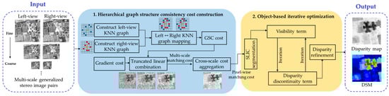
Figure 2.
The flowchart of the research methodology.
3.1. Hierarchical Graph Structure Consistency Cost Construction
In this paper, we propose a hierarchical graph structure consistency cost construction method using pixels as primitives. In the following, the hierarchical graph structure consistency cost construction is described in detail. First, the basic concept of graph structure was introduced, and then the constructed graph structure consistency cost was introduced, and finally the multi-scale GSC cost was cross-scale aggregated to output pixel-wise matching results. The overall flowchart of hierarchical graph structure consistency cost construction is shown in Figure 3.
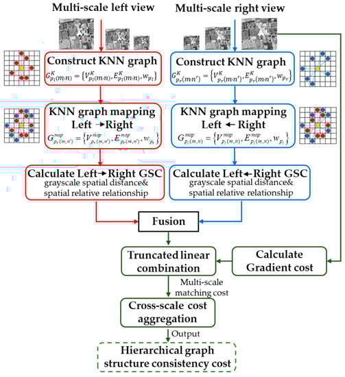
Figure 3.
The flowchart of hierarchical graph structure consistency cost construction.
3.1.1. Graph Structure
Generalized stereo image pairs are faced with radiation differences and ground feature differences brought by images from different satellites or different time phases. Radiation differences are reflected in the inconsistent grayscale distribution of the same target region, and ground feature differences are reflected in the small variations existing in image pairs, so it is meaningless to directly compare the grayscale differences of corresponding points of generalized image pairs. The graph structure can represent the structural relationship within the neighborhood of pixels, and the possibility of matching points can be judged by comparing the similarity of the graph structure. According to the self-similarity of images, a pixel in an image can always find some very similar pixels in an extended search window, and these similar pixels represent the structural information of the image, which can establish the relationship between the corresponding points of the generalized image pair. For texture-less regions, the neighborhood structure information can be obtained by adjusting the graph structure window size or reducing the image resolution. Therefore, in generalized image pairs, the neighborhood structural relationship of corresponding points was searched for, so that structural differences are presented between matching points to be comparable.
Epipolar constraints were applied to images from different satellites or different time phases, denoted as and , respectively. Here, and are the height and the width of two images, while and are the number of channels of two images. The epipolar-constrained stereo image pair was grayscaled, so = = 1. For each pixel in the left-view, the search range corresponding to the pixel in the right-view was , and represents the maximum disparity value. Here, we propose to construct a graph to represent the geometric structure for each pixel. Denoting the graph for each target pixel , we constructed the graph structure within a search window centered on as
where the term represents the distance between vertices and , and is the parameter controlling the bandwidth of the exponential kernel. Within the graph , each pixel in the search window is a vertex, and each vertex is connected to the target vertex by a set of edges . The connection weight measures the similarity between each vertex and the target vertex . The edge weight between and was generated by using the Gaussian kernel type similarity criterion.
The distance between the target vertex and all its neighbors within the search window needs to be calculated. Here, the traditional Euclidean distance was used and the normalized parameter was added.
For each pixel in the generalized image pair, the corresponding graph structure can be constructed using this operation. Since the graph structure is imaging modality invariant and insensitive to small ground feature differences and other interferences, this property was used to find the corresponding matching points in the generalized stereo image pair. Compare the structural differences between and as follows:
where , is the neighborhood point of , and is the disparity search range, . is the function of graph vertices and , such as in the simplest case, . As an effective tool for image representation and analysis, the graph model can effectively capture the key information and local structure of the image, so it was introduced into the generalized stereo matching.
3.1.2. Constructing Graph Structure Consistency Cost
Although the above criterion for calculating cost is simple and easy to understand, there is a serious risk of directly comparing the similarities between all the neighborhoods. Due to the different acquisition times of the generalized stereo image pair, there are bound to be small ground feature differences, and all neighboring pixels were used to calculate the structural differences between corresponding points, which would reduce the discriminativeness of the measurement. Meanwhile, generalized stereo image pairs have obvious illumination inconsistencies and should not be directly subtracted for comparison. Therefore, the cost calculation criterion of (4) needed to be adjusted to make it applicable to the search of matching points for generalized image pairs. On the one hand, it was necessary to determine what kind of neighborhood points were used to construct the graph structure, and on the other hand, to consider a measure method that does not directly compare the neighborhood information.
Through further observation, we found that the structural information of each pixel was concentrated on its KNN. Then, we constructed the k-nearest neighbor graph of each target pixel as
where represents the anchor pixel position set of the KNN of by sorting the distances and taking out the smallest . Instead of using all the pixels of the neighborhood, the key points characterizing the neighborhood structural information were used, effectively avoiding the interference caused by small ground feature differences on the similarity measurement of matching points. Considering the radiation differences between different satellites and different time phases, this paper does not directly compare the similarity between the corresponding point graph structures of the generalized image pairs, but maps the left-view graph structure to the corresponding neighborhood of the right-view graph structure, and compares the left-view and right-view graph structures in the same neighborhood. The mapped graph was as follows:
Figure 4 shows the process of constructing and mapping the k-nearest neighbor graph structure. The structural information of the neighborhood of the target pixel is concentrated on its KNN, and the structural difference calculated in the same neighborhood between the mapped graph and the right-view graph is to overcome the effect of radiation differences. To evaluate the differences between graph structures the GSC cost was constructed, including two measurement methods of grayscale spatial distance and spatial relative relationship. The grayscale spatial distance measurement was used to compare the differences in intensity values of key pixels between left-view and right-view graph structures, which can intuitively compare the degree of difference between the structures. Considering that there are common pixels in the graph structure, which will be offset with the calculation of grayscale spatial distance, in order to further evaluate the consistency of the graph structure, the spatial relative relationship measurement was proposed to compare the relative sizes between the common pixels and the central pixel to describe the differences between graph structures more comprehensively. The possibility of matching points was evaluated using the above two measurement methods. The GSC cost was calculated as follows:
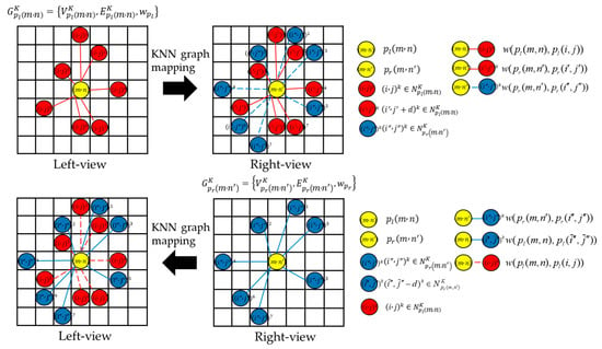
Figure 4.
The process of constructing and mapping the k-nearest neighbor graph structure.
To facilitate the acquisition of the matching cost in generalized stereo matching, the function was uniformly set to a constant 1, while the matching cost was constructed by substituting for the edge weight . The simplified GSC cost was calculated as follows:
where represents the grayscale spatial distance measurement and represents the spatial relative relationship measurement. The grayscale spatial distance measurement calculates the grayscale differences based on the rank ordering of the k-nearest neighbor pixels of the graph structure, and the spatial relative relationship measurement is used to compare the relative sizes of the common pixels and the central pixel in the graph structure. The specific formula is as follows:
where represents the coordinates of the kth neighboring pixel to in , while () represents the coordinates of the kth neighboring pixel to in . represents the common pixels of and , and and are the weights corresponding to the two measurement methods. The scale parameter of grayscale spatial distance was set to , and the scale parameter of spatial relative relationship was set to .
By calculating the structure differences between the mapped graph and the right-view graph in the same neighborhood, the direct comparison between pixels of generalized image pairs was avoided, and the interference caused by the existence of discrepant pixels on the graph structure similarity measurement was overcome. In this paper, we propose the grayscale spatial distance measurement to calculate the differences between pixel intensity values in KNN graphs, and introduce the spatial relative relationship measurement to compare the relative sizes of the common pixels and the central pixel in the graph structure to comprehensively describe the structural consistency between the mapped graph and the right-view graph .
The above steps constructed the graph structure consistency cost of mapping the left-view graph structure to the corresponding point neighborhood of the right-view, and repeated the same operation to calculate () of mapping the graph structure of the right-view to the corresponding point neighborhood of the left-view. The graph structure consistency costs and constructed by the bidirectional mapping of left-view and right-view graph structures were fused to obtain better results. In the following, the cost fusion of the graph structure bidirectional mapping was accomplished using discrete wavelet transformation and its inverse transformation. First, and were decomposed into low-frequency wavelet coefficients and , and high-frequency wavelet coefficients and (). Then, the low-frequency and high-frequency wavelet coefficients were fused as follows:
where is the Gaussian weighted local area energy coefficient defined as follows:
where is the element of the rotationally symmetric Gaussian low-pass filter of size with standard deviation . Finally, the fused GSC cost of the left-view was obtained by the inverse DWT of low-frequency and three high-frequency . Similarly, the fused GSC cost of the right-view was obtained.
Gradient information is a property of the image itself and can be used to measure the similarity of two images. Therefore, to further improve the robustness of the algorithm to interference, the gradient property of the image was added to the matching cost [34], and the gradient cost was formulated as follows:
where and represent the horizontal and vertical gradient images. The gradient images were computed using Sobel filters. The GSC cost and the gradient cost were truncated and combined with a weighted sum.
where and represent the weight parameters to balance the GSC cost and the gradient cost, and and are used to truncate the matching cost to limit the impact of outliers.
The above completes the graph structure consistency cost construction, and combines the gradient cost with strong robustness. The input of this paper is the multi-scale left-view and right-view, and the multi-scale pixel-wise matching cost can be output through the above steps. In the following, a hierarchical framework is proposed to adaptively weight and combine the multi-scale matching cost to improve the matching of texture-less regions.
3.1.3. Cross-Scale Cost Aggregation
The cross-scale cost aggregation method was proposed to improve the overall matching results by weighting and combining the multi-scale costs, while the matching of texture-less regions is also improved to some extent. Although the KNN graph can obtain the neighborhood structure information of the target pixel, it is difficult to capture the information in the texture-less region with a smooth surface on the fine scale, but it is relatively easy to capture the key structure information on the coarse scale within the same neighborhood, so the cross-scale cost aggregation was used to output the optimized pixel-wise matching results using the coarse scale matching to guide the optimization of fine scale matching. The flowchart of cross-scale cost aggregation is shown in Figure 5.

Figure 5.
The flowchart of cross-scale cost aggregation.
The literature [47] mentioned that the noisy input can usually be aggregated through (16) for the purpose of denoising. For example, the noisy matching cost can be aggregated using the cost of neighboring pixels to optimize the current pixel cost.
where denotes pixel , denotes pixel , represents disparity, and denotes , which is the neighborhood pixel of . denotes the similarity kernel, which measures the similarity between pixels and , and is the cost aggregation result. is the normalization constant. The solution of (16) is as follows:
Equation (17) is a cost aggregation process in the neighborhood on a scale, which is intra-scale cost aggregation. In order to effectively utilize the information from multiple scales to improve the matching results, the cross-scale cost aggregation method was proposed, including inter-scale cost aggregation and intra-scale cost aggregation. Cost aggregation was performed separately at multiple scales, and () denotes the matching cost of generalized stereo image pairs at different scales. The multi-scale cost was computed using downsampled images with a factor of . Note that this method also reduces the search range of disparity, and the multi-scale version of (16) is expressed as follows:
where represents the normalization constant. and denote the sequence of corresponding variables at each scale, , . denotes the neighborhood pixels of on the scale, and setting the same for all scales means that more smoothing will be performed on the coarse scale. Simultaneously, the graph structure on multi-scale images is constructed in the same neighborhood, which means that more critical information can be captured on the coarse scale. We used the vector to denote the aggregated cost at each scale. The solution of (18) is as follows:
The disparity map estimated from the cost volume at the coarser scale usually loses the disparity details, so multi-scale matching costs were adaptively combined to improve the matching results in texture-less regions while ensuring the disparity details. Here, we directly enforced the inter-scale consistency on the cost by adding a Generalized Tikhonov regularizer into (18).
where is a constant parameter to control the regularization strength, . The above is a convex optimization problem, which can be solved by finding the stationary point of the optimization target. Let represent the optimization objective of (20). For , the partial derivative of with respect to is as follows:
Let :
Set , where is a tridiagonal matrix of size and there exists an inverse matrix. The cost aggregation result on the fine scale s = 0 was as follows:
where is the intra-scale cost aggregation result, represents the weight coefficient, and then outputs the inter-scale cost aggregation result . The cross-scale cost aggregation results of left-view and right-view on the fine scale s = 0 were denoted as and .
The above is the proposed hierarchical graph structure consistency cost construction process, which is applicable to generalized stereo matching, and can improve texture-less region matching to some extent via cross-scale cost aggregation, and output pixel-wise matching results. In order to further optimize the generalized stereo matching results, iterative optimization was carried out with objects as primitives to make the algorithm more robust.
3.2. Object-Based Iterative Optimization
In the following, the output pixel-wise matching results are iteratively optimized using objects as primitives. First, the SLIC algorithm was used to perform superpixel segmentation on the image, and the output superpixel-wise cost function was as follows:
where is the number of pixels belonging to the superpixel and is the superpixel-wise cost function. Object-based cost construction can truncate outliers in pixel-wise matching to obtain stronger robustness. The following will introduce the iterative optimization process and result optimization based on the object as the primitive.
3.2.1. Iterative Optimization Based on Visibility Term and Disparity Discontinuity Term
Stereo image pairs observing the same target from different perspectives will show different facades for building targets, and the corresponding matching points cannot be searched, that is, there are occluded regions. The pixels located in occlusion regions cannot observe a ground truth matching point, and the wrong disparity value may affect the optimization of the neighboring superpixels. Therefore, occlusion needs to be detected, and this part of the region is not processed, but the neighborhood information is used for optimization. To solve the occlusion problem, a visibility term was defined to determine whether it was an occluded superpixel by the left-right consistency check, where occluded superpixels had no match on the target image and unoccluded superpixels had at least one match.
where and represent the current disparity maps of the left-view and right-view images, and and are the and centroids of the superpixel . The occlusion of superpixels was judged by (25) and the detection results were vectorized as . The matching costs were multiplied by the validation vector:
where represents the number of superpixels, represents the element-wise product function, , and represents the matching cost of the iteration update.
Disparity discontinuity regions inevitably exist in remote sensing images, and the disparity discontinuity is usually located at the junction of the foreground and background, such as a roof and façade, or a roof and the ground. In the process of optimizing the matching results, a disparity discontinuity term was proposed to prevent the smoothness penalty from blurring the disparity boundary. The boundary disparity was optimized by calculating the difference between the current superpixel disparity and the neighboring superpixel weighted disparity and assigning different penalties, thus maintaining the intensity difference between neighboring superpixels. Neighboring superpixel weighted disparity was calculated as follows:
where represents the index of the superpixel within the neighborhood of the superpixel, is the result of the left-right consistency check, is the optimal disparity of the neighboring superpixel in the current state, and is the neighboring superpixel weighted disparity. represents the similarity of two neighboring superpixels, which was calculated as follows:
where and are the intensities of the and superpixels, and are parameters that control the shape of the function, and we set and according to experience. The intensity of a superpixel was calculated by averaging the intensities of all pixels it contains.
The disparity discontinuity term was calculated using the current superpixel disparity and the neighboring superpixel weighted disparity. A robustness penalty function was introduced, defined as
where represents the scaling parameter and represents the truncation parameter; these two parameters play an important role in controlling the robustness penalty function, which were empirically set as and . The truncation parameter represents the difference between the current superpixel disparity and the neighboring superpixel weighted disparity.
The proposed disparity discontinuity term preserved the disparity boundary by maintaining the intensity difference between neighboring superpixels. The abnormal disparity values in the disparity smoothing region were improved by increasing the cost of incorrect disparity values and decreasing the cost of correct disparity values through a constant penalty. For regions where disparity boundaries are prone to mismatching, the mis-matched superpixels usually have large differences between the disparity and the neighborhood weighted disparity due to over-smoothing, and the matching result was corrected by penalizing to increase the cost of the incorrect disparity, and then gradually approximating the correct disparity. The disparity discontinuity term optimizes the boundary disparity results to avoid blurring the details of the target into the background. Meanwhile, the penalty function prevents model overfitting to reduce the cases of falling into unfavorable local minimums.
In the following, the proposed visibility term and the disparity discontinuity term are iteratively optimized to continuously detect occlusions and optimize the boundary disparity. The proposed algorithm iteratively updated the matching cost as follows, and set the iteration termination condition as .
where weight matrix contains the edge weights, and is obtained by normalizing the rows of . represents the disparity discontinuity term of the iteration, represents the visibility term of the iteration, is used to balance the disparity discontinuity term and the visibility term, with the weight parameter set empirically, and represents the matching cost after the update. The number of iterations was set to , and the number of superpixels was set to .
The iterative update optimization process introduced above takes objects as primitives, detects the occlusion using the visibility term, and calculates the relationship between the current superpixel disparity and the neighboring superpixel weighted disparity using the disparity discontinuity term, and then assigns a different penalty to the current superpixel to improve the disparity in the transition region between the foreground and the background.
3.2.2. Disparity Refinement
After further improving the occlusion and disparity discontinuity regions, the fractal net evolution method [48] was introduced to merge homogeneous superpixels to constrain the disparity results in order to better characterize the ground feature boundary information. The fractal net evolution method is a bottom-up region growing method that merges smaller objects based on an optimization function, and the merging criterion is that the spectral heterogeneity and shape heterogeneity of the new objects do not exceed user-defined thresholds. The above results were optimized using the fractal net evolution method to output a more complete and accurate disparity map.
3.3. IOHGSCM
The IOHGSCM algorithm is summarized as Algorithm 1.
| Algorithm 1 IOHGSCM |
| Input: Epipolar constrainted left image Ileft and right image Iright |
| Output: Disparity map dIOHGSCM and digital surface model DSMIOHGSCM |
| 1 /* Hierarchical graph structure consistency cost construction */ |
| 2 Obtain left-view KNN graph and right-view KNN graph by setting ws and K |
| 3 Obtain graph structure consistency cost (left→right) and (left←right) |
| 4 Fusion of the and |
| 5 Truncated and weighted combination of GSC cost and gradient cost |
| 6 Obtain multi-scale cost |
| 7 Add a generalized Tikhonov regularizer into Equation (18) |
| 8 Obtain multi-scale cost aggregation result |
| 9 /* Object-based iterative update optimization */ |
| 10 Obtain superpixel segmentation cost function F(s,d) by SLIC |
| 11 for 1 ≤ t + 1 ≤ nInter do |
| Set |
| Compute , |
| Compute |
| end |
| 12 Optimize disparity map using fractal net evolution |
4. Results
In this section, qualitative and quantitative experiments are carried out on the public US3D dataset and self-made dataset. We conducted experiments on generalized stereo image pairs from different satellites or different time phases. In the following, the parameters and evaluation metrics used in this paper are described, the proposed method is compared with the state-of-the-art stereo matching methods, and the effectiveness of the proposed method in hierarchical graph structure consistency cost construction, and object-based iterative optimization is demonstrated. The parameters used for the proposed algorithm are listed in Table 2.
Table 2.
Parameter settings for the experiments.
4.1. Evaluation Metrics
The output disparity map was calculated using RFM to obtain DSM, and the generated DSM was compared with the ground truth DSM. In this paper, two evaluation metrics were used to verify the accuracy of the DSM generated by the proposed method and the comparison methods, including the root mean square error (RMSE) [49] and the normalized median absolute deviation (NMAD) [50].
RMSE was used to measure the error between the predicted DSM and the true DSM. The smaller the RMSE, the more accurate the reconstructed result. The RMSE was calculated as follows:
where represents the number of test points, and and represent the true DSM and predicted DSM.
NMAD can better solve the problem of heavy tails in the error distribution due to more outliers, and is a robust evaluation method for estimating Δh. The NMAD was calculated as follows:
where () represents the individual error and is the median of the errors. Therefore, NMAD is proportional to the median of the absolute value of the difference between the individual error and the median error. It is considered as a more resilient estimation method for data outliers.
4.2. Effectiveness of Hierarchical Graph Structure Consistency Cost Construction
In the following, the effectiveness of the hierarchical graph structure consistency cost construction will be demonstrated. The effectiveness of the constructed GSC + Gradient cost is demonstrated on the one hand, and the improvement of the proposed hierarchical framework on the matching results is demonstrated on the other hand. Figure 6 compares the intensity value distribution of the generalized stereo image pairs on the same target. The analysis of the distribution of intensity values on the surface of multiple targets (in-cluding building targets, ground targets) shows that there are obvious radiation differ-ences in the generalized image pairs, large differences in the intensity values of the same target points, large differences in the degree of intensity variation between the same target points, and roughly similar trends in intensity value fluctuations between sampling points on the same target. Simultaneously, there are different trends among some sampling points, which are considered as fluctuating variations caused by small ground feature differences. Therefore, it is necessary to design a cost construction method suitable for generalized stereo matching.
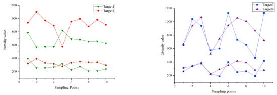
Figure 6.
Comparison of intensity value distribution of generalized image pairs on the same target.
The constructed graph structure consistency cost takes into account the small ground feature differences and does not use all the pixels in the neighborhood for comparison, but designs a KNN graph characterizing the target pixel neighborhood structural information. Considering the radiation differences, this paper maps the left-view and right-view graph structures to the same neighborhood for comparison. To demonstrate the effectiveness of the proposed graph structure consistency cost, the combination of GSC and gradient cost was compared with the commonly used combination of census transform and gradient cost [34], and color and gradient cost [38], where the two measurements of the above cost combination were truncated and combined with a weighted sum. This paper verified the effectiveness of GSC cost construction on seven datasets, and the experimental results are shown in Table 3. The experimental results of the seven datasets showed that the DSM predicted by GSC + Gradient had a smaller prediction error and less outlier distribution, which effectively improved the matching between pixels. The constructed GSC cost is robust across multiple datasets, and for generalized image pairs of different satellites or different time phases, GSC + Gradient performed better than Census + Gradient, and even better than Color + Gradient. Census is a matching method that is robust to illumination changes. Census uses Hamming distance to calculate the consistency of the relative relationship between the neighboring pixels and the central pixel of two images, it uses all pixels in the neighborhood without taking into account small variations of ground features. Meanwhile, it only considers the relative relationship between the neighboring pixels and the central pixel, and does not consider the grayscale difference and distance relationship between the neighboring pixels and the central pixel, which affects the matching accuracy in some aspects, so Census + Gradient performed poorly in generalized stereo matching. However, Color + Gradient also failed to obtain a better correspondence of pixels by directly using the grayscale information of the two images without considering the matching problem caused by radiation differences. The above experiments demonstrated the effectiveness of the graph structure consistency cost construction.
Table 3.
Performance of different cost construction methods on multiple datasets.
The proposed hierarchical framework weighted a combination of multi-scale matching costs; fine scale, due to the close gray value of texture-less regions, finds it difficult to characterize the neighborhood structure information from the graph structure, while coarse scale can better characterize the target pixel neighborhood structure information, using coarse scale matching to guide the optimization of fine scale matching to improve the matching results of texture-less regions to a certain extent. Figure 7 and Table 4 show the disparity maps and reconstruction accuracy generated by different scales and multi-scale cost aggregation, respectively. For dataset 2 and dataset 3, the texture-less phenomenon of the building target is obvious, and the top surface gray value of the building target is close, which makes it difficult to find the corresponding matching points. Therefore, this paper takes dataset 2 and dataset 3 as examples, and the red boxes mark the texture-less regions. On dataset 2 and dataset 3, there were dark black regions on the building top surface on the fine scale, and the disparity of this region was small, showing different disparity results from other regions on the building top surface. For the same building top surface, the disparity is continuous and the variation is small, indicating that there were obvious matching errors on the building top surface in these regions. As the scale changes from fine to coarse, it was obvious that the coarse scale can capture more structural information in the same neighborhood, and the matching results of the building top surface in the red box were gradually improved. The reconstruction results were compared using two evaluation parameters, RMSM and NMAD, and it was found that the matching results on scale 2 were better for the stereo image pairs where the texture-less phenomenon is more obvious, and the reconstruction results were further improved by cross-scale cost aggregation. The experimental results show that the proposed hierarchical framework not only improves the overall reconstruction accuracy using a weighted combination of multi-scale costs, but also improves the matching results in texture-less regions. Through the subsequent object-based iterative optimization process, a smoother disparity result on the top surface of the building can be obtained.
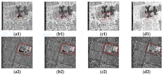
Figure 7.
Disparity maps generated using graph structure consistency (GSC) + Gradient at different scales and multi-scale cost aggregation. Dataset 2 (a1) Scale 1, (b1) Scale 2, (c1) Scale 3, (d1) Aggregation; Dataset 3 (a2) Scale 1, (b2) Scale 2, (c2) Scale 3, (d2) Aggregation.
Table 4.
Comparison of reconstruction results at different scales and multi-scale cost aggregation.
The effectiveness of the proposed hierarchical graph structure consistency cost construction is demonstrated experimentally, which can improve the texture-less regions to some extent. The above outputs’ pixel-wise matching results, and the effectiveness of the object-based iterative optimization process will be demonstrated.
4.3. Effectiveness of Object-Based Iterative Optimization
In order to optimize the pixel-wise matching results, iterative optimization using objects as primitives was proposed to make the algorithm more robust, which continuously detects occlusion and optimizes the disparity in the transition region between foreground and background through iteration. The visibility term was defined to determine whether it was an occluded superpixel via a left–right consistency check. The disparity discontinuity term calculated the difference between the current superpixel disparity and the neighboring superpixel weighted disparity and assigned different penalties, thus maintaining the intensity difference between neighboring superpixels to optimize the boundary disparity. Finally, the fractal net evolution was used to constrain the ground feature boundaries to further optimize the disparity results and output a complete and accurate disparity map.
To demonstrate the effectiveness of the object-based iterative optimization process, the output pixel-wise matching results were compared with the matching results after object-based iterative optimization on seven datasets, and the corresponding DSMs were generated using RFM to compare the effect of the object-based iterative optimization process on the stereo reconstruction results. Table 5 shows the RMSE/NMAD changes of the reconstruction results on the seven datasets before and after the object-based iterative optimization. After the object-based iterative optimization, the reconstruction accuracy on all seven datasets obtained a significant improvement. The improvement in the reconstruction results was larger for dataset 1, dataset 2, dataset 3, and dataset 6, and the RMSE was improved by 3–5 m. The improvement in the reconstruction results was smaller for dataset 4, dataset 5, and dataset 7, and the RMSE was improved by 0.6–1 m. There are complexly distributed buildings and high-rise buildings in dataset 1, dataset 2, dataset 3, and dataset 6. Theoretically, at different observation angles, the higher the building target, the larger the occluded region, and the more complex the building distribution, the more disparity discontinuity regions. Therefore, the pixel-wise matching results can be improved using the proposed object-based iterative optimization. The building patterns in dataset 4, dataset 5, and dataset 7 are low and monotonous, and a better pixel-wise matching result was obtained through the constructed hierarchical graph structure consistency cost, so the improvement in the reconstruction results after object-based iterative optimization was relatively small. In summary, the experiments demonstrated the effectiveness of object-based iterative optimization, which is suitable for occlusion detection and boundary disparity optimization.
Table 5.
Comparison of reconstruction results before and after object-based iterative optimization.
4.4. Comparison with State-of-the-Art
Due to the different acquisition times of the generalized stereo image pairs, there are obvious radiation differences and small ground feature differences. We carried out the following research on the radiation inconsistency, texture-less and repetitive patterns, and occlusion and disparity discontinuity regions in the generalized stereo matching process. Several typical stereo reconstruction methods, including SGM [18], ARWSM [34], MeshSM [12], FCVFSM [11], HMSMNet [24], DSMNet [25], BGNet [21], StereoNet [20] were used for comparison with the proposed stereo reconstruction method. This paper reproduced these methods based on their open-source code. In order to compare the performance of different stereo reconstruction methods, we set the disparity range to be consistent with the proposed method. In the following, we will analyze the performance of the proposed method and several comparative methods on seven datasets.
Radiation inconsistencies between generalized stereo image pairs, as well as the presence of texture-less and repetitive patterns, and occlusion and disparity discontinuity regions make stereo matching difficult. To address the above issues, several stereo image pairs containing typical scenes were selected to evaluate the performance of different stereo reconstruction methods.
Radiation inconsistency regions. For images acquired from different satellites or different times, there will inevitably be radiation differences, and inconsistent grayscale distribution of the same target region in stereo image pairs will make matching difficult. The proposed method uses the bi-directional mapping of the graph structure to calculate the matching cost, effectively overcoming matching errors caused by radiation inconsistencies and small ground feature differences. Figure 8 shows the reconstruction results of the proposed method and the mainstream methods in the radiation inconsistency regions (dataset 1). The experimental results showed that the proposed method can better match the corresponding pixels of the stereo image pairs in the radiation inconsistency region, and the reconstruction results were closer to ground truth (GT), better preserving the target details and having a better target contour. The four non-deep learning methods had more noisy regions in the reconstruction results; it was impossible to obtain more complete and accurate reconstruction results for complex building targets, and the target contour was blurred. The four deep learning methods performed averagely in the stereo reconstruction of generalized image pairs, with small ground feature details blurred into the background, and for more complex scenes, there were more matching errors on typical targets and less clear boundary contours. The above experimental results showed that the proposed method is suitable for the reconstruction of radiation inconsistency regions.
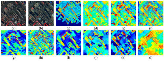
Figure 8.
The reconstruction results of the proposed method and mainstream methods in the radiation inconsistency regions (dataset 1). (a) Left image; (b) right image; (c) ground truth (GT); (d) iterative optimization of hierarchical graph structure consistency cost (IOHGSCM); (e) ARWSM; (f) SGM; (g) MeshSM; (h) FCVFSM; (i) HMSMNet; (j) DSMNet; (k) StereoNet; (l) BGNet.
Texture-less and repetitive pattern regions. The weak variation of pixel intensity in the texture-less region makes it difficult to distinguish pixels, leading to ambiguous results. Meanwhile, image patches in repetitive patterns regions have similar structures and appearances, leading to blurred matching. The proposed hierarchical graph structure consistency cost will improve the matching results of texture-less and repetitive patterns regions to some extent. Figure 9 shows the reconstruction results of the proposed method and the mainstream methods in the regions of texture-less and repetitive patterns. There are obvious texture-less regions in dataset 3 and dataset 7 on the top surface of the building target. The proposed method performed better in the texture-less region, and the reconstruction results of the target region were more complete and retained more detailed information. In dataset 3, BGNet performed better, and the reconstruction results were relatively complete and closer to ground truth (GT), while the remaining three deep learning methods performed unsatisfactorily in the texture-less region. Meanwhile, the targets in the reconstruction results of ARWSM and SGM were more complete, but there was more noise in SGM. In dataset 7, the proposed method performed optimally, and the building targets were relatively complete in the reconstruction results of several mainstream methods. There was excessive smoothing in the reconstruction results of several deep learning methods, which blurred the details of the target, and the reconstruction results of the trees around the building were poor. Meanwhile, several non-deep-learning methods, such as ARWSM and MeshSM, performed better, and there was more noise in the reconstruction results of SGM and FCVFSM. There are obvious repetitive patterns in dataset 4, where the features and contours of the building targets are similar. For repetitive patterns regions, the non-deep-learning method ARWSM performed better with clearer and more accurate target contours. Among the deep learning methods, DSMNet and BGNet performed well, with better reconstruction results for building targets, but the reconstruction results for trees were not accurate enough. The above experimental results showed that the proposed method can be better applied to texture-less and repetitive pattern regions.
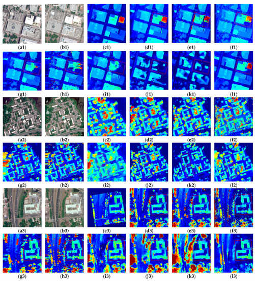
Figure 9.
The reconstruction results of the proposed method and mainstream methods in the regions of texture-less and repetitive patterns (dataset 3, dataset 4, dataset 7). (a1–a3) Left image; (b1–b3) right image; (c1–c3) GT; (d1–d3) IOHGSCM; (e1–e3) ARWSM; (f1–f3) SGM; (g1–g3) MeshSM; (h1–h3) FCVFSM; (i1–i3) HMSMNet; (j1–j3) DSMNet; (k1–k3) StereoNet; (l1–l3) BGNet.
Disparity discontinuities and occlusions. Disparity discontinuities will lead to the well-known edge-fattening issue. However, the existence of an occlusion will not be able to find a corresponding match and the disparity can only be approximated. Such phenomena are ubiquitous in satellite imagery due to tall objects and elevation discontinuities. Figure 10 shows the reconstruction results of the proposed method and the mainstream methods in the regions of occlusion and disparity discontinuity. The proposed method performed better in regions with complex building distributions, and the stereo information of the target region was well reconstructed with relatively clear contours. Among the non-deep-learning methods, ARWSM performed better in dataset 2, dataset 5, and dataset 6. SGM performed well in dataset 2, while in dataset 5 and dataset 6, it did not perform well for the reconstruction of complexly distributed building clusters or building targets with relatively complex backgrounds, and there was more noise in the reconstruction results. MeshSM and FCVFSM performed poorly in the stereo reconstruction of disparity discontinuity regions. Among the deep learning methods, BGNet performed better in occlusion and disparity discontinuity regions, with clear contours of the ground features, but the reconstruction results had the phenomenon of edge-fattening compared with GT. The remaining three deep-learning methods suffered from over-smoothing, which blurred the details of ground features into the background, and performed poorly in the reconstruction of vegetation regions. The above experimental results showed that the proposed method can improve the reconstruction results of occlusion and disparity discontinuity regions to some extent.
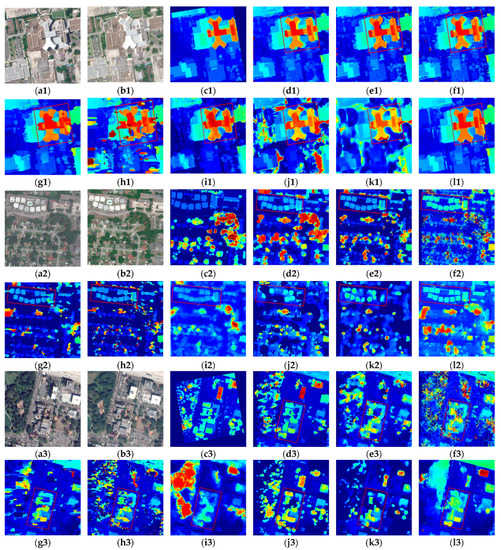
Figure 10.
The reconstruction results of the proposed method and mainstream methods in the regions of occlusion and disparity discontinuity (dataset 2, dataset 5, dataset 6). (a1–a3) Left image; (b1–b3) right image; (c1–c3) GT; (d1–d3) IOHGSCM; (e1–e3) ARWSM; (f1–f3) SGM; (g1–g3) MeshSM; (h1–h3) FCVFSM; (i1–i3) HMSMNet; (j1–j3) DSMNet; (k1–k3) StereoNet; (l1–l3) BGNet.
In this paper, both RMSE and NMAD were used to evaluate the accuracy of the reconstruction results of seven generalized image pairs from different satellites or different time phases on multiple methods. Table 6 and Table 7 show the RMSE and NMAD comparisons of the reconstruction results of the proposed method and mainstream methods in different datasets, respectively. In dataset 1 (different satellites and different time phases), the proposed IOHGSCM had obvious advantages compared with other methods in RMSE and NMAD, achieving an RMSE/NMAD of 4.31 m/2.41 m, outperforming several non-deep-learning methods by 1.63 m/1.03 m (RMSE/NMAD) and outperforming several deep learning methods by 2.04 m/1.78 m (RMSE/NMAD). For dataset 1, the non-deep-learning methods had more accurate reconstruction results and smaller deviations than the deep learning methods. The non-deep-learning method ARWSM performed better, the deep learning method BGNet performed better, and the overall performance of several deep learning methods was average. For the satellite stereo reconstruction task, due to the complex distribution of ground features, there is a lack of a large number of training samples to train the deep learning network, and the training process is time-consuming, which is not suitable for real-scene 3D application requirements. In dataset 2-dataset 7 (different time phases), the proposed IOHGSCM can achieve the optimal reconstruction results, with approximately 2.93 m/2.01 m (RMSE/NMAD) as compared with ARWSM (3.31 m/2.11 m), SGM (3.97 m/2.68 m), MeshSM (3.77 m/2.42 m), FCVFSM (4.44 m/2.93 m), BGNet (3.31 m/2.26 m), HMSMNet (4.05 m/2.72 m), DSMNet (4.19 m/2.92 m), and StereoNet (4.62 m/3.37 m). In dataset 2-dataset 7, the non-deep-learning method ARWSM performed best and the deep learning method BGNet performed best. The root mean square error (RMSE) of the reconstruction results of BGNet was close to that of ARWSM, while the deviation of the reconstruction results of ARWSM was better than that of BGNet. In dataset 3, BGNet performed slightly better than IOHGSCM, and BGNet performed better in texture-less regions. In dataset 5, the NMAD of ARWSM was slightly better than that of IOHGSCM, indicating that the deviation of the reconstruction results of ARWSM in disparity discontinuity regions was less floating and the algorithm was relatively stable. In dataset 7, the NMAD of MeshSM was slightly better than that of IOHGSCM, and the reconstruction results were relatively stable in the texture-less region. The experimental results on seven datasets showed that the proposed method performed well overall, and had obvious reconstruction advantages in relatively complex scenes, effectively overcoming the effects of radiation differences and ground feature differences in generalized image pairs, and improving the reconstruction results of texture-less and disparity discontinuity regions to a certain extent, which is an effective and reliable generalized stereo matching method for urban 3D reconstruction, and provides technical support for the stereo reconstruction of multi-view satellite images.
Table 6.
Root mean square error (RMSE) comparison of the reconstruction results of the proposed method and mainstream methods in different datasets.
Table 7.
Normalized median absolute deviation (NMAD) comparison of the reconstruction results of the proposed method and mainstream methods in different datasets.
5. Discussion
5.1. Comparison of Algorithm Time Consumption
The proposed algorithm was compared with the mainstream methods in terms of time consumption, and the experimental results are shown in Table 8. IOHGSCM, ARWSM, SGM, MeshSM and FCVFSM were run on Window 10, Intel i7-7700 CPU 3.6 GHz. HMSMNet, DSMNet, BGNet and StereoNet were run on Ubuntu 20.04, Python 3.7, CUDA 11.2, cuDNN 8.1.1, GTX 1080 GPU. Among the non-deep-learning methods, ARWSM and SGM have faster running times of 8.99 s and 6.83 s, and the proposed method has a running time of 19.12 s, which outperforms MeshSM (27.22 s) and FCVFSM (45.56 s). The four deep-learning methods trained the model in advance, and the time consumption of BGNet for data testing was 1.13 s, which outperforms DSMNet (2.02 s), StereoNet (2.17 s), and HMSMNet (3.92 s). The proposed method does not require pre-trained models, which is suitable for situations with relatively complex scenes and without too many training samples to obtain more reliable and accurate stereo matching results, while the time consumption of the algorithm is within an acceptable range.
Table 8.
Comparison of the time consumption of the proposed method and mainstream methods.
5.2. Parameter Selection for KNN Graph
In this paper, we proposed a generalized stereo matching method based on an iterative optimization of a hierarchical graph structure consistency cost for urban 3D scene reconstruction. The constructed GSC cost is critical. In the following, we will analyze the choice of parameters , , , , , and in detail. Parameter determines the neighborhood of the target pixel. A large choice of will increase the time consumption significantly, while a small choice will not represent the graph structure well. Parameter determines the number of similar pixels within the neighborhood of the target pixel. According to the self-similarity of the image, these similar pixels represent the structural information within the neighborhood of the target pixel.
In order to balance the algorithm time consumption with the reconstruction accuracy, we set parameter with a step size of 2 and parameter , where with a step size of 0.1. Parameters , , , were set as above. In order to select the optimal parameters and guarantee the time consumption of the proposed algorithm, the window size was not set too large. Figure 11 and Figure 12 show the RMSE and NMAD of the predicted DSM under different window sizes and different k-nearest neighbor parameters (take dataset 1 as an example). The experimental results showed that different and affect the matching of the corresponding pixels in the two images. In the following, parameter was used to represent parameter . With a fixed window size , RMSE and NMAD showed a trend of first rising and then decreasing with the increase in (). With the increase in , on scale 1 and scale 2, RMSE and NMAD showed a relatively large decrease and then tended to fluctuate steadily, while on scale 3, RMSE and NMAD showed a large trend of decrease and then increased slowly. The increase in can enhance the description of the neighborhood structure of the target pixel to some extent. When is too large, not only does it greatly increase the running time of the algorithm, but also comes with the risk of introducing interfering information, leading to a tendency for accuracy to fluctuate or even decrease.
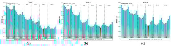
Figure 11.
The change in RMSE corresponding to the predicted digital surface model (DSM) with different parameters of ws and K for the GSC cost construction method. (a) Scale 1; (b) Scale 2; (c) Scale 3.
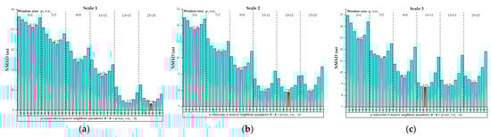
Figure 12.
The change in NMAD corresponding to the predicted DSM with different parameters ws and K for the GSC cost construction method. (a) Scale 1; (b) Scale 2; (c) Scale 3.
In summary, on scale 1, the optimal parameters were and , considering that the smaller and , the lower the computational complexity, and as the evaluation parameters (RMSE and NMAD) of the reconstruction results corresponding to and were close, we set and . On scale 2, and performed optimally, when , RMSE and NMAD fluctuated less and tended to be flat, so we set and . On scale 3, and performed optimally. The experimental results showed that the variation trend of and were almost identical on several scales, and the optimal values of the parameters and were stabilized at and , respectively. The window size was still larger on the coarse scale, indicating that more structural information is contained in the corresponding neighborhood, which is helpful for the matching of texture-less regions. When the evaluation parameters RMSE and NMAD are close, smaller and should be chosen to further reduce the time consumption of the algorithm while ensuring the reconstruction results. The choice of and facilitates the construction of graph structure consistency cost and provides a good start for subsequent steps.
5.3. Evaluation of IOHGSCM
In order to effectively evaluate the proposed method, we conduct detailed analysis on representative targets in several datasets. Figure 13 shows the comparison between the proposed method and the mainstream methods in the reconstruction results of typical target regions. There are radiation differences, occlusions, and disparity discontinuities in the six target regions. Target 1, target 2, and target 6 are stereo image pairs from different satellites and different time phases, and there are obvious radiation differences. The weak texture on the top surface of the building target in target 3, target 4, and target 5 is more obvious. When observing building targets from different perspectives, the six groups of target regions will show different facades, resulting in occluded regions and a large degree of disparity variation at the junction of a roof and facade, or a roof and the ground, resulting in disparity discontinuity regions.
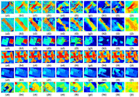
Figure 13.
Comparison between the reconstruction results of the proposed method and mainstream methods in typical target regions. (a1–a6) GT; (b1–b6) IOHGSCM; (c1–c6) ARWSM; (d1–d6) SGM; (e1–e6) MeshSM; (f1–f6) FCVFSM; (g1–g6) HMSMNet; (h1–h6) DSMNet; (i1–i6) StereoNet; (j1–j6) BGNet.
By comparing the reconstruction results of the various methods shown in Figure 13, we found that among the deep learning methods, HMSMNet, DSMNet, and StereoNet performed poorly in the stereo matching of generalized image pairs, with incomplete target reconstruction results and blurred target contours. There was also over-smoothing, and there were more mismatched regions. BGNet performed relatively well on stereo image pairs of different time phases, and the target reconstruction results were more complete and accurate, but had the phenomenon of edge-fattening. For stereo image pairs of different satellites and different time phases, the performance of BGNet was relatively poor, with blurred target contours and more mismatches. In target 4, the building target reconstruction results of BGNet had the phenomenon of edge-fattening, which is due to the fact that the network cannot handle the information of the occluded building facade better, and the building facade matching error causes the edge-fattening of the target reconstruction results. The performance of ARWSM and SGM among the non-deep-learning methods was relatively stable, but there were more noisy regions, while the target reconstruction results obtained by MeshSM and FCVFSM were poor, with more mismatched regions, incomplete target reconstruction results, and large deviations from GT. ARWSM performed better among the non-deep-learning methods, and BGNet performed better among the deep learning methods. Target 6 belongs to the small target; only the proposed method can better reconstruct the stereo information of the target and maintain the boundary of the target. The remaining stereo reconstruction methods were less effective for the reconstruction of small building targets in the generalized image pairs, and the reconstruction results were fuzzy and incomplete. The proposed method obtained more accurate and reliable reconstruction results on several target regions with clearer target contours.
Table 9 and Table 10 show the comparison of RMSE and NMAD of the reconstruction results for typical target regions on multiple stereo reconstruction methods, respectively. Among the six groups of target regions, the proposed method had better reconstruction results than the remaining eight mainstream methods, and the RMSE/NMAD of the reconstruction results was 3.69 m/2.13 m. Among the non-deep-learning methods, the reconstruction results of ARWSM (4.97 m/2.78 m) and SGM (5.28 m/2.92 m) were relatively stable and can be better applied to multiple scenes. Among the deep learning methods, BGNet (4.72 m/2.80 m) performed well, but there were some anomalous matching results around the building targets. The proposed method was qualitatively and quantitatively analyzed with the results of mainstream stereo reconstruction methods, further proving that the proposed IOHGSCM is an accurate and reliable generalized stereo matching scheme adapted to urban 3D reconstruction.
Table 9.
RMSE comparison of the reconstruction results of the proposed method and mainstream methods in typical target regions.
Table 10.
NMAD comparison of the reconstruction results of the proposed method and mainstream methods in typical target regions.
6. Conclusions
This paper proposes a novel generalized stereo matching method based on the iterative optimization of a hierarchical graph structure consistency cost for urban 3D scene reconstruction. This paper consists of two main parts, one is hierarchical graph structure consistency cost construction with pixels as primitives, and the other is iterative optimization with objects as primitives. In the first part, the KNN graph is first constructed. Structural difference is calculated through the bi-directional mapping of the graph structure. Then, using cross-scale cost aggregation to adaptively combine multi-scale costs, the matching in texture-less regions is effectively improved, and the pixel-wise matching results are output. In the second part, the matching cost is optimized iteratively using the visibility term and the disparity discontinuity term. The experimental results show that the constructed GSC + Gradient achieves an RMSE/NMAD of 7.33 m/5.59 m on multiple datasets, which is better than Census + Gradient (8.71 m/6.79 m) and Color + Gradient (9.28 m/7.53 m), indicating that the proposed cost construction method is applicable to the stereo matching of generalized image pairs. This paper also demonstrates the effectiveness of the hierarchical framework weighted combination of multi-scale cost and object-based iterative optimization for the improvement of reconstruction results. Comparing the proposed IOHGSCM with eight mainstream stereo reconstruction methods on seven datasets, including four deep learning methods and four non-deep-learning methods, the RMSE/NMAD of the proposed IOHGSCM on multiple datasets is 3.13 m/2.06 m, which is better than four non-deep-learning methods by 1.04 m/0.60 m, and better than four deep learning methods by 1.24 m/0.95 m. The average running time of the four non-deep-learning methods is 22.15 s, among which ARWSM and SGM run faster, and MeshSM and FCVFSM run relatively slower. For the four deep learning methods that have pre-acquired trained models, the average time for testing data is 2.31 s, while the running time of the proposed method is 19.12 s, which is within an acceptable range. In summary, the experimental results show that IOHGSCM provides an effective and reliable method for generalized image pair stereo reconstruction.
The research on the stereo reconstruction method of generalized image pairs provides the possibility to obtain stereo information of arbitrary regions and provides a technical basis for the research of stereo matching based on high-resolution multi-view satellite images. In the future, we will further conduct research on multi-view satellite image stereo reconstruction, which involves optical images from different time phases and different satellites. Research on the complementary technology of multi-view image information and the impact of resolution differences between different images on matching results will be carried out to obtain comprehensive and accurate stereo information of the target region. Meanwhile, primitive model matching and texture mapping are also the focus of future research in order to meet the demand of urban 3D real-scene construction.
Author Contributions
Methodology, S.Y.; Software, S.Y.; Validation, S.Y.; Formal analysis, S.Y.; Investigation, W.C.; Resources, H.C.; Data curation, W.C.; Writing—original draft, S.Y.; Writing—review & editing, S.Y.; Visualization, W.C.; Supervision, H.C.; Project administration, H.C.; Funding acquisition, H.C. All authors have read and agreed to the published version of the manuscript.
Funding
This work was supported in part by the Natural Science Foundation of Heilongjiang Province under Grant YQ2021F005, and in part by the National Key Laboratory of Science and Technology on Remote Sensing Information and Image Analysis Foundation Project under Grant 6142A0103011.
Data Availability Statement
Not applicable.
Conflicts of Interest
The authors declare no conflict of interest.
References
- Li, Y.; Wu, B. Relation-constrained 3D reconstruction of buildings in metropolitan areas from photogrammetric point clouds. Remote Sens. 2021, 13, 129. [Google Scholar] [CrossRef]
- Qi, Z.; Zou, Z.; Chen, H. 3D Reconstruction of Remote Sensing Mountain Areas with TSDF-Based Neural Networks. Remote Sens. 2022, 14, 4333. [Google Scholar] [CrossRef]
- Stathopoulou, E.K.; Welponer, M.; Remondino, F. Open-source image-based 3D reconstruction pipelines: Review, comparison and evaluation. ISPRS-Int. Arch. Photogramm. Remote Sens. Spat. Inf. Sci. 2019, 42, 331–338. [Google Scholar] [CrossRef]
- Xiao, X.; Guo, B.; Li, D.; Li, L.; Yang, N.; Liu, J.; Zhang, P.; Peng, Z. Multi-view stereo matching based on self-adaptive patch and image grouping for multiple unmanned aerial vehicle imagery. Remote Sens. 2016, 8, 89. [Google Scholar] [CrossRef]
- Nguatem, W.; Mayer, H. Modeling urban scenes from Pointclouds. In Proceedings of the IEEE International Conference on Computer Vision (ICCV), Venice, Italy, 22–29 October 2017; pp. 3857–3866. [Google Scholar]
- Wohlfeil, J.; Hirschmüller, H.; Piltz, B.; Börner, A.; Suppa, M. Fully automated generation of accurate digital surface models with sub-meter resolution from satellite imagery. Int. Arch. Photogramm. Remote Sens. Spat. Inf. Sci. 2012, XXXIX-B1, 75–80. [Google Scholar] [CrossRef]
- Pan, C.; Liu, Y.; Huang, D. Novel belief propagation algorithm for stereo matching with a robust cost computation. IEEE Access 2019, 7, 29699–29708. [Google Scholar] [CrossRef]
- Mozerov, M.G.; Van De Weijer, J. Accurate stereo matching by twostep energy minimization. IEEE Trans. Image Process. 2015, 24, 1153–1163. [Google Scholar] [CrossRef]
- Liu, H.; Wang, R.; Xia, Y.; Zhang, X. Improved cost computation and adaptive shape guided filter for local stereo matching of low texture stereo images. Appl. Sci. 2020, 10, 1869. [Google Scholar] [CrossRef]
- Zhang, B.; Zhu, D. Local stereo matching: An adaptive weighted guided image filtering-based approach. Int. J. Pattern Recognit. Artif. Intell. 2021, 35, 2154010. [Google Scholar] [CrossRef]
- Hosni, A.; Rhemann, C.; Bleyer, M.; Rother, C.; Gelautz, M. Fast cost-volume filtering for visual correspondence and beyond. IEEE Trans. Pattern Anal. Mach. Intell. 2013, 35, 504–511. [Google Scholar] [CrossRef]
- Zhang, C.; Li, Z.; Cheng, Y.; Cai, R.; Chao, H.; Rui, Y. Meshstereo: A global stereo model with mesh alignment regularization for view interpolation. In Proceedings of the IEEE International Conference on Computer Vision, Santiago, Chile, 13–16 December 2015; pp. 2057–2065. [Google Scholar]
- Hallek, M.; Boukamcha, H.; Mtibaa, A.; Atri, M. Dynamic programming with adaptive and self-adjusting penalty for real-time accurate stereo matching. J. Real-Time Image Process. 2022, 19, 233–245. [Google Scholar] [CrossRef]
- Nguyen, P.H.; Ahn, C.W. Stereo Matching Methods for Imperfectly Rectified Stereo Images. Symmetry 2019, 11, 570–590. [Google Scholar]
- Shin, Y.; Yoon, K. PatchMatch belief propagation meets depth upsampling for high-resolution depth maps. Electron. Lett. 2016, 52, 1445–1447. [Google Scholar] [CrossRef]
- Zeglazi, O.; Rziza, M.; Amine, A.; Demonceaux, C. A hierarchical stereo matching algorithm based on adaptive support region aggregation method. Pattern Recognit. Lett. 2018, 112, 205–211. [Google Scholar] [CrossRef]
- Haq, Q.M.U.; Lin, C.H.; Ruan, S.J.; Gregor, D. An edge-aware based adaptive multi-feature set extraction for stereo matching of binocular images. J. Ambient. Intell. Humaniz. Comput. 2022, 13, 1953–1967. [Google Scholar] [CrossRef]
- Hirschmuller, H. Stereo processing by semiglobal matching and mutual information. IEEE Trans. Pattern Anal. Mach. Intell. 2008, 30, 328–341. [Google Scholar] [CrossRef]
- Yang, W.; Li, X.; Yang, B.; Fu, Y. A Novel Stereo Matching Algorithm for Digital Surface Model (DSM) Generation in Water Areas. Remote Sens. 2020, 12, 870. [Google Scholar] [CrossRef]
- Khamis, S.; Fanello, S.; Rhemann, C.; Kowdle, A.; Valentin, J.; Izadi, S. StereoNet: Guided Hierarchical Refinement for Real-Time Edge-Aware Depth Prediction. In Proceedings of the European Conference on Computer Vision (ECCV), Munich, Germany, 8–14 September 2018; pp. 573–590. [Google Scholar]
- Xu, B.; Xu, Y.; Yang, X.; Jia, W.; Guo, Y. Bilateral grid learning for stereo matching network. arXiv 2021, arXiv:abs/2101.01601. [Google Scholar]
- Zhao, L.; Liu, Y.; Men, C.; Men, Y. Double Propagation Stereo Matching for Urban 3-D Reconstruction from Satellite Imagery. IEEE Trans. Geosci. Remote Sens. 2021, 60, 1–17. [Google Scholar] [CrossRef]
- Tatar, N.; Arefi, H.; Hahn, M. High-Resolution Satellite Stereo Matching by Object-Based Semiglobal Matching and Iterative Guided Edge-Preserving Filter. IEEE Geosci. Remote Sens. Lett. 2020, 18, 1841–1845. [Google Scholar] [CrossRef]
- He, S.; Li, S.; Jiang, S.; Jiang, W. HMSM-Net: Hierarchical multi-scale matching network for disparity estimation of high-resolution satellite stereo images. ISPRS J. Photogramm. Remote Sens. 2022, 188, 314–330. [Google Scholar] [CrossRef]
- He, S.; Zhou, R.; Li, S.; Jiang, S.; Jiang, W. Disparity Estimation of High-Resolution Remote Sensing Images with Dual-Scale Matching Network. Remote Sens. 2021, 13, 5050. [Google Scholar] [CrossRef]
- Chen, W.; Chen, H.; Yang, S. Self-Supervised Stereo Matching Method Based on SRWP and PCAM for Urban Satellite Images. Remote Sens. 2022, 14, 1636. [Google Scholar] [CrossRef]
- Zhang, C.; Cui, Y.; Zhu, Z.; Jiang, S.; Jiang, W. Building Height Extraction from GF-7 Satellite Images Based on Roof Contour Constrained Stereo Matching. Remote Sens. 2022, 14, 1566. [Google Scholar] [CrossRef]
- Nemmaoui, A.; Aguilar, F.J.; Aguilar, M.A.; Qin, R. DSM and DTM generation from VHR satellite stereo imagery over plastic covered greenhouse areas. Comput. Electron. Agric. 2019, 164, 104903. [Google Scholar] [CrossRef]
- Wang, W.; Song, W.; Liu, Y. Precision analysis of 3D reconstruction model of generalized stereo image pair. Sci. Surv. Mapp. 2010, 35, 31–33. [Google Scholar]
- Yan, Y.; Su, N.; Zhao, C.; Wang, L. A Dynamic Multi-Projection-Contour Approximating Framework for the 3D Reconstruction of Buildings by Super-Generalized Optical Stereo-Pairs. Sensors 2017, 17, 2153. [Google Scholar] [CrossRef]
- Aguilar, M.A.; Saldaña, M.M.; Aguilar, F.J. Generation and Quality Assessment of Stereo-Extracted DSM From GeoEye-1 and WorldView-2 Imagery. IEEE Trans. Geosci. Remote Sens. 2014, 52, 1259–1271. [Google Scholar] [CrossRef]
- Liu, B.; Yu, H.; Qi, G. GraftNet: Towards Domain Generalized Stereo Matching with a Broad-Spectrum and Task-Oriented Feature. In Proceedings of the IEEE/CVF Conference on Computer Vision and Pattern Recognition, New Orleans, LA, USA, 19–24 June 2022; pp. 13012–13021. [Google Scholar]
- Zhang, J.; Wang, X.; Bai, X.; Wang, C.; Huang, L.; Chen, Y.; Hancock, E.R. Revisiting Domain Generalized Stereo Matching Networks from a Feature Consistency Perspective. In Proceedings of the IEEE/CVF Conference on Computer Vision and Pattern Recognition, New Orleans, LA, USA, 19–24 June 2022; pp. 13001–13011. [Google Scholar]
- Lee, S.; Jin, H.L.; Lim, J.; Suh, I.H. Robust stereo matching using adaptive random walk with restart algorithm. Image Vis. Comput. 2015, 37, 1–11. [Google Scholar] [CrossRef]
- Sun, J.; Zheng, N.N.; Shum, H.Y. Stereo matching using belief propagation. IEEE Trans. Pattern Anal. Mach. Intell. 2003, 25, 787–800. [Google Scholar]
- Fei, L.; Yan, L.; Chen, C.; Ye, Z.; Zhou, J. Ossim: An object-based multiview stereo algorithm using ssim index matching cost. IEEE Trans. Geosci. Remote Sens. 2017, 99, 6937–6949. [Google Scholar] [CrossRef]
- Liang, Z.; Feng, Y.; Guo, Y.; Liu, H.; Qiao, L.; Chen, W.; Zhang, J. Learning deep correspondence through prior and posterior feature constancy. arXiv 2017, arXiv:1712.01039. [Google Scholar]
- Li, S.; Chen, K.; Song, M.; Tao, D.; Chen, G.; Chen, C. Robust efficient depth reconstruction with hierarchical confidence-based matching. IEEE Trans. Image Process. 2017, 26, 3331–3343. [Google Scholar]
- Bosch, M.; Foster, K.; Christie, G.; Wang, S.; Hager, G.D.; Brown, M. Semantic stereo for incidental satellite images. In Proceedings of the 2019 IEEE Winter Conference on Applications of Computer Vision (WACV), Waikoloa Village, HI, USA, 7–11 January 2019; pp. 1524–1532. [Google Scholar]
- Zhang, D.; Xie, F.; Zhang, L. Preprocessing and fusion analysis of GF-2 satellite Remote-sensed spatial data. In Proceedings of the 2018 International Conference on Information Systems and Computer Aided Education (ICISCAE), Changchun, China, 6–8 July 2018; IEEE: Piscataway, NJ, USA, 2018; pp. 24–29. [Google Scholar]
- Huang, B.; Zheng, J.; Giannarou, S.; Elson, D.S. H-Net: Unsupervised Attention-based Stereo Depth Estimation Leveraging Epipolar Geometry. In Proceedings of the IEEE/CVF Conference on Computer Vision and Pattern Recognition, New Orleans, LA, USA, 19–24 June 2022; pp. 4460–4467. [Google Scholar]
- Wang, Y.; Lu, Y.; Lu, G. Stereo Rectification Based on Epipolar Constrained Neural Network. In Proceedings of the IEEE International Conference on Acoustics, Speech and Signal Processing, Toronto, ON, Canada, 6–11 June 2021; pp. 2105–2109. [Google Scholar]
- Yi, H.; Chen, X.; Wang, D.; Du, S.; Xu, B.; Zhao, F. An Epipolar Resampling Method for Multi-View High Resolution Satellite Images Based on Block. IEEE Access 2021, 9, 162884–162892. [Google Scholar] [CrossRef]
- Fuhry, M.; Reichel, L. A new Tikhonov regularization method. Numer. Algorithms 2012, 59, 433–445. [Google Scholar] [CrossRef]
- Achanta, R.; Shaji, A.; Smith, K.; Lucchi, A.; Fua, P.; Süsstrunk, S. SLIC Superpixels Compared to State-of-the-Art Superpixel Methods. IEEE Trans. Pattern Anal. Mach. Intell. 2012, 34, 2274–2282. [Google Scholar] [CrossRef] [PubMed]
- Gholinejad, S.; Amiri-Simkooei, A.; Moghaddam, S.H.A.; Naeini, A.A. An automated PCA-based approach towards optization of the rational function model. ISPRS J. Photogramm. Remote Sens. 2020, 165, 133–139. [Google Scholar] [CrossRef]
- Zhang, K.; Fang, Y.Q.; Min, D.B.; Sun, L.F.; Yang, S.Q.; Yan, S.C.; Tian, Q. Cross-Scale Cost Aggregation for Stereo Matching. IEEE Trans. Circuits Syst. Video Technol. 2017, 27, 965–976. [Google Scholar] [CrossRef]
- Hu, Z.; Wu, Z.; Zhang, Q.; Fan, Q.; Xu, J. A Spatially-Constrained Color-Texture Model for Hierarchical VHR Image Segmentation. IEEE Geosci. Remote Sens. Lett. 2013, 10, 120–124. [Google Scholar] [CrossRef]
- Liu, J.; Zhang, L.; Wang, Z.; Wang, R. Dense Stereo Matching Strategy for Oblique Images That Considers the Plane Directions in Urban Areas. IEEE Trans. Geosci. Remote Sens. 2020, 58, 5109–5116. [Google Scholar] [CrossRef]
- Höhle, J.; Höhle, M. Accuracy assessment of digital elevation models by means of robust statistical methods. ISPRS J. Photogramm. Remote Sens. 2009, 64, 398–406. [Google Scholar] [CrossRef]


Disclaimer/Publisher’s Note: The statements, opinions and data contained in all publications are solely those of the individual author(s) and contributor(s) and not of MDPI and/or the editor(s). MDPI and/or the editor(s) disclaim responsibility for any injury to people or property resulting from any ideas, methods, instructions or products referred to in the content. |
© 2023 by the authors. Licensee MDPI, Basel, Switzerland. This article is an open access article distributed under the terms and conditions of the Creative Commons Attribution (CC BY) license (https://creativecommons.org/licenses/by/4.0/).