Deep-Learning-Based Semantic Segmentation Approach for Point Clouds of Extra-High-Voltage Transmission Lines

Abstract

The accurate semantic segmentation of point cloud data is the basis for their application in the inspection of extra high-voltage transmission lines (EHVTL). As deep learning evolves, point-wise-based deep neural networks have shown great potential for the semantic segmentation of EHVTL point clouds. However, EHVTL point cloud data are characterized by a large data volume and significant class imbalance. Therefore, the down-sampling method and point cloud feature extraction method used in current point-wise-based deep neural networks hardly meet the needs of computational accuracy and efficiency. In this paper, we proposed a two-step down-sampling method and a point cloud feature extraction method based on local feature aggregation of the point clouds after down-sampling in each layer of the model (LFAPAD). We then established a deep neural network named PowerLine-Net for the semantic segmentation of the EHVTL point clouds. Furthermore, in order to test and analyze the performance of PowerLine-Net, we constructed a point cloud dataset for the EHVTL scenes. Using this dataset and the Semantic3D dataset, we implemented network parameter testing, semantic segmentation, and an accuracy comparison of different networks based on PowerLine-Net. The results illustrate that the semantic segmentation model proposed in this paper has a high computational efficiency and accuracy in the semantic segmentation of EHVTL point clouds. Compared with conventional deep neural networks, including PointCNN, KPConv, SPG, PointNet++, and RandLA-Net, PowerLine-Net also achieves a higher accuracy in the semantic segmentation of EHVTL point clouds. Moreover, based on the results predicted by PowerLine-Net, the risk point detection for EHVTL point clouds has been achieved, which demonstrates the important value of this network in practical applications. In addition, as shown by the results of Semantic3D, PowerLine-Net also achieves a high segmentation accuracy, which proves its powerful capability and wide applicability in semantic segmentation for the point clouds of large-scale scenes.

1. Introduction

The normal operation of an extra-high-voltage transmission line (EHVTL) is significant in guaranteeing the power supply for daily production and life. With the continuous expansion of power networks [1] and the increasing demand for electricity, the safety and reliability requirements of EHVTLs have increased. Given the complex structure and large number of components of EHVTLs, they are likely to have equipment failures. Therefore, the periodic inspection of EHVTLs [2] has become an essential task for the power supply industry.

In current EHVTL inspections, the point clouds of EHVTLs acquired by airborne LiDAR technology have become the main form of data [3,4,5]. In terms of data processing, accurate semantic segmentation for point clouds is the basis of various applications, such as risk point detection [6,7], 3D visualization [8], conductor measurements [9,10], conductor arc sag, ice cover, wind deflection analysis, and so on. However, compared to manual or point cloud library methods, deep learning has shown great potential in the field of the semantic segmentation of point clouds due to its high processing efficiency and ability to extract data features autonomously, thus attracting extensive attention from scholars [11,12].

The mainstream deep neural networks for the semantic segmentation of point clouds are divided into three main categories: voxel-based networks [13,14], multi-view-based networks [15,16,17,18], and point-based networks [19]. Among them, point-based networks do not require data transformation during feature learning and completely retain the original information of point clouds [19], which can utilize the point cloud information accurately and directly, thus enhancing accuracy in semantic segmentation.

The current point-based networks are further divided into (1) point-convolution-based networks, such as the PointCNN proposed by Li et al. [20], which employs the farthest point down-sampling (FPS) method, processes the initial features of the point cloud based on “X-Conv”, and then performs a convolution calculation to obtain the features of the input point cloud, and the KPConv model proposed by Thomas et al. [21], which adapts the convolution kernel to the point cloud geometry features by performing local displacement learning from the input radius neighborhood; (2) graph-based networks, such as a network based on superpoint graphs (SPGs) proposed by Landrieu et al. [22], which first spatially divides the input point clouds to obtain a series of geometric partitions, treats each geometric partition as a superpoint, then employs a graph convolutional neural network to learn the contextual features, and finally obtains the features of the geometric partition corresponding to the superpoint; and (3) point-wise-based networks, such as the PointNet [19], PointNet++ [23], Stratified Transformer [24], and Pointnext [25], which all adopt the FPS method. The RandLA-Net [26], SCF-Net [27], and GA-NET [28] all use the random down-sampling (RS) strategy, which has significant computational efficiency advantages over networks based on the FPS method and has achieved better application results on several public large-scale point cloud datasets. Clearly, point-wise-based networks have the advantages of a simple logical structure and direct point-wise feature learning and can avoid a large number of convolutional calculations compared with other methods. Thus, point-wise-based networks can be popularly applied in the semantic segmentation of EHVTL point clouds [29].

According to the related works, we found that, in order to be applicable to EHVTL data with a large data volume, sparse point clouds, and significant class imbalance, point-wise-based methods still need further improvement in the following two aspects: achieving efficient and accurate semantic segmentation for point clouds. For down-sampling methods, in which the commonly used down-sampling methods in point-wise-based networks are FPS [19,23,24,25] and RS [26,27,28]. The FPS method can only process small-scale point cloud data because it cannot consider both computational efficiency and memory occupation, whereas the RS method tends to sample unevenly, resulting in information loss in categories with a low number of points. For point cloud feature extraction methods, such as the MLP-based method in PointNet++ [23], there exist a high computational complexity and weak extraction capability for local features [30,31]. In contrast, the feature extraction method based on the point clouds before down-sampling each layer of RandLA-Net [26] needs to calculate the features of all points and requires twice-dilated residual block calculations, which introduce additional computational effort.

In addition, constructing point cloud datasets that can accurately reflect the target features is the basis for achieving high-precision point cloud semantic segmentation based on deep learning. Given the discrepancies in the dataset features of different scenes, the datasets of indoor scenes mainly reflect indoor features (e.g., tables and chairs), whereas the datasets of outdoor scenes mainly contain urban or field features (e.g., buildings). Therefore, the appropriate dataset should be selected according to the requirements of practical applications. Several typical public point cloud datasets have emerged for different semantic segmentation tasks, such as ModelNet [32], ScanNet [33], Semantic3D [34], KITTI [35], WHU-TLS [36], WHU-MLS [37], and so on. However, the conventional public dataset cannot accurately reflect the point cloud data features of EHVTL scenes mainly due to the following: (1) the conventional point cloud dataset contains fewer scenes of power lines, and they are mostly urban or rural low-voltage power lines, but very few contain EHVTL scenes; (2) class imbalance in a single EHVTL scene (i.e., the middle area of two pylons) is obvious, especially regarding the number of ground points accounting for a huge proportion whereas the number of points in other categories such as conductors accounting for a relatively small proportion; and (3) the ground situation in the EHVTL scenes is complex; for example, vegetation, buildings, low-voltage transmission lines, and other features in the field environment have complex structures and are severely overshadowed by each other. Therefore, a corresponding point cloud dataset should be established to realize the semantic segmentation of the EHVTL point cloud data based on deep neural networks.

In summary, we focused on the semantic segmentation of the EHVTL point cloud dataset based on deep neural networks. We first improved the current point-wise-based deep neural networks (RandLA-Net) in terms of down-sampling methods and the point cloud feature extraction method for feature encoding, proposed a down-sampling method based on two-step down-sampling (TS) and a feature extraction method based on local feature aggregation of the point clouds after down-sampling in each layer (LFAPAD), and then built a deep neural network for the semantic segmentation of EHVTL point clouds—PowerLine-Net. Meanwhile, in order to verify the effectiveness of PowerLine-Net in the semantic segmentation of EHVTL point cloud data, we established a deep learning dataset using the EHVTL point cloud data acquired based on airborne LiDAR. Furthermore, the performance of the network proposed in this paper was tested based on our dataset and the public dataset—Semantic3D. Through this research, we aimed to provide an efficient and reliable method to support the data processing of EHVTL point clouds.

2. Network Architecture

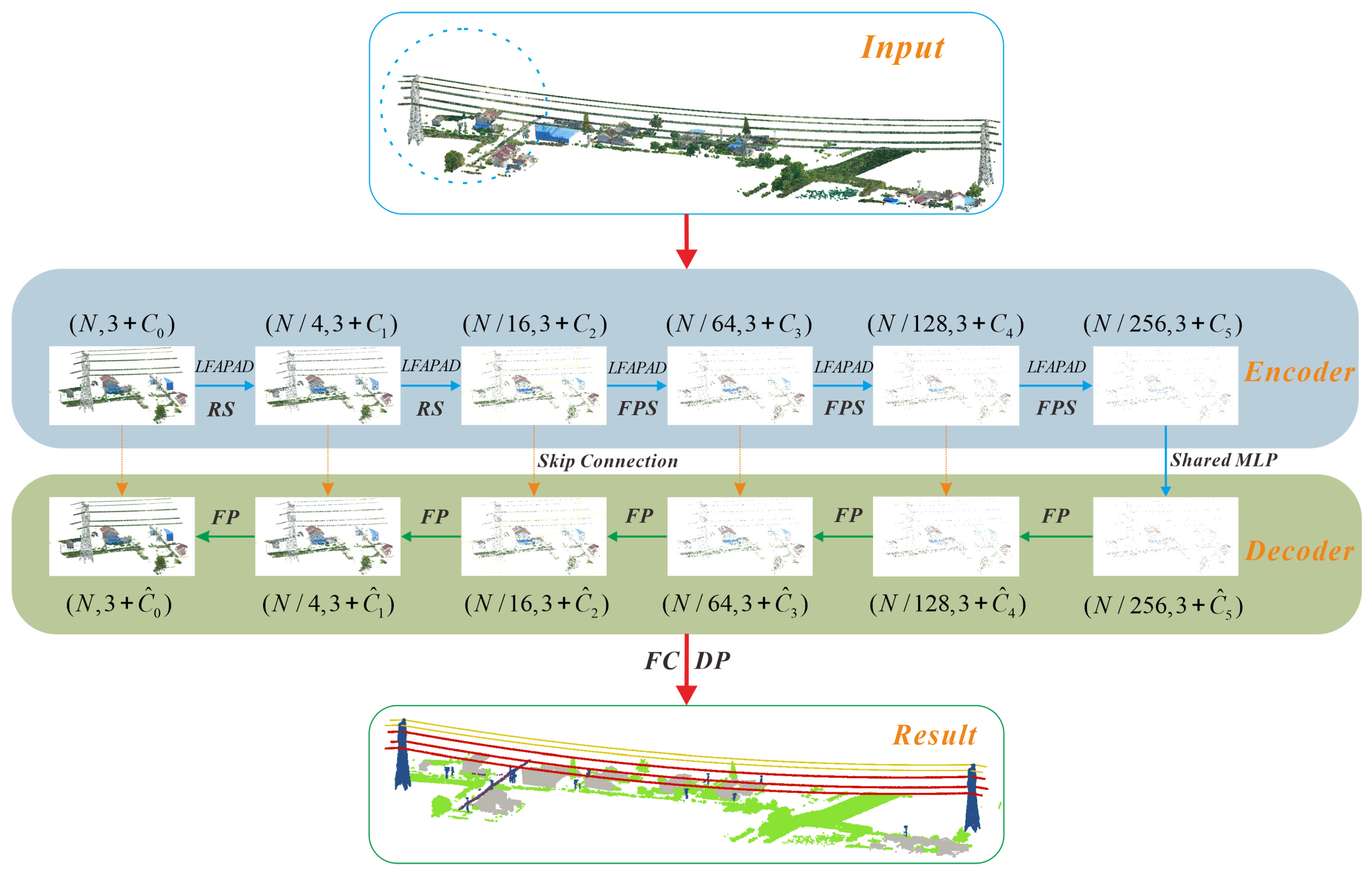
The core of a deep-learning-based point cloud semantic segmentation network is firstly training the network by learning features through the encoding and decoding layers. Then, the network is tested based on the test dataset. During this process, feature encoding is the key for the entire algorithm to efficiently extract representable point cloud features. At present, the point-wise-based deep neural network has the advantages of a simple logical structure and retaining more point cloud information compared with other methods; hence, it is highly suitable for the semantic segmentation of large-scene point clouds. However, the point clouds of the EHVTL scene are characterized by a large data volume, sparsity of point clouds, and significant class imbalance. Thus, the down-sampling method and the point cloud feature extraction method commonly used in the current feature encoding of point-wise-based deep neural networks can hardly satisfy the needs of their computational efficiency and semantic segmentation accuracy. To address these problems, we proposed a TS method and a feature extraction method based on LFAPAD in the process of feature encoding. On this basis, we built a deep neural network for the semantic segmentation of EHVTL point clouds, and its structure is shown in Figure 1. The encoding layer mainly includes a two-step down-sampling method and local feature aggregation method.

2.1. Two-Step Down-Sampling

An efficient and accurate down-sampling method is crucial to the feature encoding process during point cloud down-sampling. At present, two down-sampling methods are mainly used in point-wise-based deep neural networks: RS and FPS. The computational complexity of RS and FPS are O(1) [26] and O(N~10⁶) [26], respectively. The RS method tends to lose point cloud features in the sampling process, and it is not suitable for the feature extraction of sparse point clouds, but its computational efficiency does not decrease as the number of down-sampling points increases; FPS has an exponential increase in computational cost with an increase in down-sampling points, but it can preserve the key geometric information of the data extremely well during the down-sampling [26]. In addition, too many layers of random down-sampling or setting too high down-sampling rates for the farthest point down-sampling can lead to the loss of point cloud features. In order to consider both efficiency and accuracy, we adopted a multi-scale combined sampling method (i.e., the two-step method) for the characteristics of EHVTL point cloud data. For example, in the five-layer feature encoding structure, we employed the RS method in the first two layers with a 25% down-sampling rate for both layers, and the FPS method with 25%, 50%, and 50% down-sampling rates in the last three layers.

Given that the number of initial input point clouds is large, RS can effectively reduce the number of points and improve the computational efficiency. Based on a significant reduction in the number of points, the FPS can achieve uniform sampling and effectively retain the information of sparse point clouds, which is beneficial to the extraction of accurate geometric features of point clouds [37].

2.2. Local Feature Aggregation after Down-Sampling

Since the down-sampling process of deep neural networks tends to lose some information about key point clouds (such as edge points, curvature change points, local maximum points, etc.), the geometric feature extraction of point cloud data is required during feature encoding to preserve as much point cloud information as possible. Local feature aggregation [26] is a recognized feature extraction method that can effectively preserve geometric details. However, it performs feature computation in the point cloud before down-sampling in each layer of the model. The features cannot completely transmit to the next layer after down-sampling, which inevitably introduces extra computational effort. Therefore, we adopted the feature extraction method based on LFAPAD as shown in Figure 2. In each layer of the model, the method considers the points after down-sampling as local center points, obtains their abstract features, calculates the relevant position information with un-sampled point clouds, and finally aggregates all of the information to obtain the local features of each center point.

The feature extraction process in this paper includes nearest neighbor query, relative position feature calculation, feature pooling, feature mapping, and so on. We took any point $p_i^m$ in a set of points $P_i=\left\{p_i^1,p_i^2,\cdots ,p_i^{n_i}\right\},p_i^n\in {ℝ}^{\left(3+d_i\right)}(n=1,2,\dots n_i)$ ($n_i$ denotes the number of points in the ith layer; $d_i$ denotes the dimension of features other than coordinates, such as RGB, etc.) of the ith layer as an example, where the coordinate value of $p_i^m$ is $a_{i,m}$. According to Section 2.1, $P_i$ is obtained by down-sampling from the $P_{i-1}$ of the (i − 1)th layer. Based on the k-nearest neighbor (KNN) algorithm [38], we obtained the KNN coordinates $l_{i,m}=\left\{l_{i,m}^1,l_{i,m}^2,\cdots ,l_{i,m}^k\right\}$, and the point feature $f_{i,m}=\left\{f_{i,m}^1,f_{i,m}^2,\cdots ,f_{i,m}^k\right\},f_{i,m}^b\in {ℝ}^{d_i}(b=1,2,\dots k)$ (see relative feature in Figure 2) of the $p_i^m$ from $P_{i-1}$, calculated the relative spatial positional information between points $r_{i,m}=\left\{r_{i,m}^1,r_{i,m}^2,\cdots ,r_{i,m}^k\right\},r_{i,m}^b\in {ℝ}^{{d_i}^{\prime }}(b=1,2,\dots k)$, (${d_i}^{\prime }$ denotes the total length of the concatenation of the feature dimensions, ${d_i}^{\prime }=10$) (see relative position in Figure 2) between the KNN and the center point using Equation (1), and obtained the local nearest neighbor feature ${\widehat{f}}_{i,m}=\left\{{\widehat{f}}_{i,m}^1,{\widehat{f}}_{i,m}^2,\cdots ,{\widehat{f}}_{i,m}^k\right\}$ by mapping the correlation position information to the nearest neighbor feature through the mapping function $g(r_{i,m},f_{i,m})$ as shown in Equation (2). The formula for MLPs is Equation (3).

$$r_{i,m}^j=\left(a_{i,m}\oplus l_{i,m}^j\oplus \left(a_{i,m}-l_{i,m}^j\right)\oplus ||a_{i,m}-l_{i,m}^j||\right),j=1,2,\cdots k$$

(1)

In the above equation, $\oplus$ denotes concatenation and $\left|\right|.\left|\right|$ denotes Euclidean distance.

$${\widehat{f}}_{i,m}=g(r_{i,m},f_{i,m})=MLPs(r_{i,m})\oplus f_{i,m}$$

(2)

$$M^s=\sigma \left(w^s{M}^{s-1}+b^s\right)$$

(3)

In the above equation, $\mathsf{\oplus }$ denotes the weight matrix of the sth layer of MLP, $M^{s-1}$ denotes the output of the (s – 1)th layer of MLP, $b^s$ denotes the bias of the sth layer of MLP, $\sigma$ denotes the activation function, and $\sigma$ is ReLU in our network.

After obtaining the local nearest neighbor feature ${\widehat{f}}_{i,m}$ of the point $p_i^m$, pooling was then performed to obtain the single-point aggregation feature $c_{i,m}\in {ℝ}^{1\times d_{out}}$. The current common methods for local nearest neighbor feature pooling are max pooling and average pooling; however, they commonly suffer from the problem of missing key features in the neighborhood in their applications [26]. In order to avoid this problem, we utilized the adaptive pooling strategy [26]; that is, in the local feature pooling calculation for each center point, the corresponding attention score $s_{i,m}=\left\{s_{i,m}^1,s_{i,m}^2,\cdots ,s_{i,m}^k\right\}$ was calculated for each nearest neighbor feature based on the shared perceptron and $s_{i,m}$ was calculated as shown in Equation (4).

$$s_{i,m}=h({\widehat{f}}_{i,m},w)=softmax(MLPs({\widehat{f}}_{i,m},w))$$

(4)

In Equation (4), $w$ denotes the learnable weights of the shared MLP, which are obtained by learning and used to perform adaptive pooling operations on the features to achieve the down-sampling of the point clouds. $h({\widehat{f}}_{i,m},w)$ is the mapping function, and $s_{i,m}$ is used as a mask for labeling key features and then weighted summation with the local nearest neighbor feature ${\widehat{f}}_{i,m}$. The result was then mapped to higher dimensions using the MLPs to obtain the pooling result $c_{i,m}$ shown in Equation (5).

$$c_{i,m}=MLPs\left[{\displaystyle \sum }_{j=1}^k\left(s_{i,m}^j\odot {\widehat{f}}_{i,m}^j\right)\right]$$

(5)

In the above formula, $\odot$ denotes the Hadamard product. Finally, after point-wise calculation, the features $c_i=\left\{c_{i,1},c_{i,2},\cdots ,c_{i,n_i}\right\},c_{i,n}\in {ℝ}^{n_i\times d_{out}}(n=1,2,\dots n_i)$ of the point clouds after down-sampling were obtained and used as the point features of the (i + 1)th layer.

2.3. Network Structure of PowerLine-Net

In order to achieve the semantic segmentation of EHVTL point clouds, based on the point-wise-based deep neural network, we adopted the TS method and the feature extraction method based on LFAPAD to construct a deep neural network—PowerLine-Net. The architecture of PowerLine-Net mainly consists of the following four parts:

(1) Data input (Input): Divide the point cloud data (training dataset or test dataset) into chunks according to certain rules (for EHVTL point cloud data, certain rules are the division of two adjacent pylons and the area between the pylons into a section), and subsequently input each chunk of data into the network as a training sample or test sample. Given that the data size of EHVTL point clouds is too large to be used as a sample input network for training, the point cloud data should be divided, and the input sample data for the network should be built. Commonly used networks, such as PointNet++ and PointConv, divide the point cloud of the whole scene into fixed sizes, where the partially overlapping point cloud blocks the preprocessing stage, which are used as input samples for subsequent network training and testing. This approach is intuitive; however, the fixed-sized division tends to lose the structural information of the features, making it difficult for the network to effectively learn the geometric structure information of the features during training. In order to address the above-mentioned problems, we used a sample point selection method based on category weights and distance weights which can improve the completeness of the same object in the input data. The specific calculation steps of the algorithm are as follows:

(a)

Assigning each point in the data set a random value in the range of $[0,1\times {10}^{-3}]$ as the initial screening value.

(b)

Taking the point with the smallest screening value within the data set as the centroid and then adding minimal perturbation to the screening value of that centroid.

(c)

Obtaining the $N$ closest points around this centroid as a single sample data using the KNN search algorithm. $N$ denotes the number of points in a single sample data.

(d)

Calculating the category weights of the selected sample points within the dataset to which they belong. The category weight for each point of the training dataset is set to the ratio of the number of points in the category corresponding to that point to the total number of points and that of the test dataset is set to 1. The screening value of each point is then updated using Equation (6).

$$s=s+(1-\frac{dis}{\max (dis)})w$$

(6)

where $s$ indicates the screening value, $dis$ indicates the distance between the selected sample points and the center point, and $w$ indicates the category weight.

(e)

Repeating the above steps until the number of sample data required for a single training is obtained.

(2) Feature encoding (Encoder): This contains a five-layer network structure. In terms of down-sampling, we applied the TS method; that is, the first two encoding layers reduce the number of points using RS, and the final three encoding layers reduce the number of points using FPS. In terms of feature extraction based on LFAPAD, we obtained the geometric structure information of point clouds into the encoded feature. This process mainly reduces the number of points, increases the feature dimension of each point, and then aggregates the features of all sample points into the sampled sparse sample points.

(3) Feature decoding (Decoder): This also contains a five-layer network structure. From the feature encoding process, the number of points is significantly reduced after the down-sampling process and the point cloud feature extraction, whereas the local features of the point clouds are aggregated to a very low number of sample points; however, the feature information of each point in the original input data cannot be obtained. Therefore, the network should back-propagate the small number of sample point features obtained from the feature encoding process to each point of the original input data; this process is called feature decoding. In this process, the point cloud from feature encoding is first mapped onto the feature decoding layer using MLPs, and the network then uses the nearest neighbor interpolation method to transfer the features extracted from the sparse point cloud after sampling to the dense point cloud before sampling. The skip connection method is also used during the propagation of features in each layer of the model, where it also uses the skip connection method [26] to linearly superimpose the features after interpolation with the corresponding encoded features obtained from the feature encoding for each sampled point. The main purpose of this process is to propagate the high-dimensional aggregated features from the sampled sparse point cloud to each point of the input data.

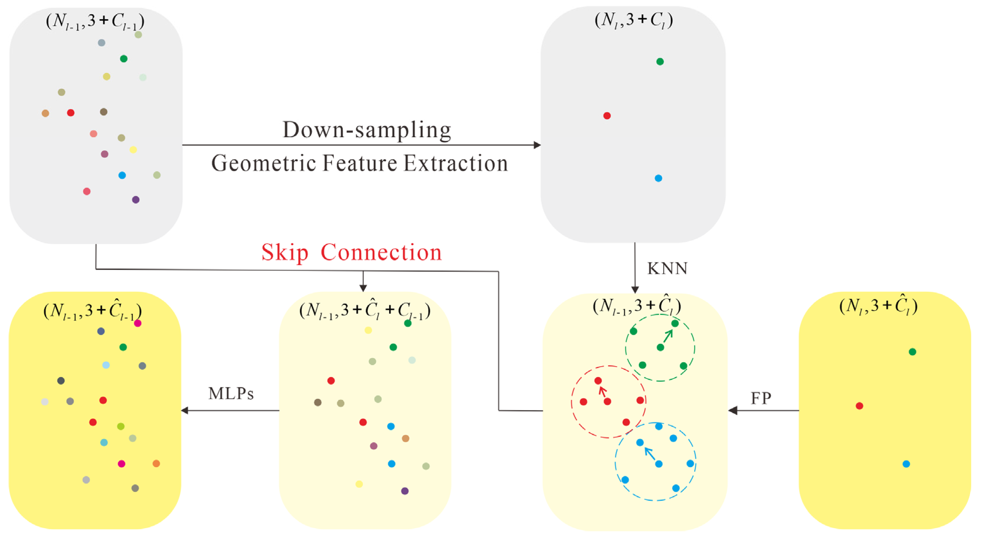
The following part takes the $l$th layer network as an example to illustrate the feature decoding process, as shown in Figure 3. The point clouds with feature size $(N_{l-1},3+C_{l-1})$ can be abstracted into the point clouds $(N_l,3+C_l)$ through the down-sampling and feature extraction processes, and the input feature size for the feature decoding layer is $(N_l,3+{\widehat{C}}_l)$. First, we considered the $N_l$ points as the center points and obtained the k nearest points from the $N_{l-1}$ points based on the KNN algorithm. In feature propagation (FP), we transferred the features of each center point to the selected nearest points and obtained the point clouds $(N_{l-1},3+{\widehat{C}}_l)$. The skip connection was then used to connect the point clouds $(N_{l-1},3+C_{l-1})$ and $(N_{l-1},3+{\widehat{C}}_l)$ to obtain the point clouds $(N_{l-1},3+{\widehat{C}}_l+C_{l-1})$. Finally, we used the MLPs to transform the point clouds $(N_{l-1},3+{\widehat{C}}_l+C_{l-1})$ to $(N_{l-1},3+{\widehat{C}}_{l-1})$, thus achieving the $l$th layer feature decoding. By analogy, the five-layer feature decoding process can be achieved.

(4) Prediction output (Result): Based on the features of the input sample data obtained from the feature decoding process, we used full concatenation and dropout to reduce the feature dimension of each point to the number of categories, and then obtained the probability of each sample point belonging to different categories with the activation function. Finally, the category with a higher probability value is the predicted category for each point.

The architecture of PowerLine-Net is shown in Figure 4.

3. EHVTL Dataset Construction

Deep learning is a data-driven technique; hence, datasets are the foundation for the training and testing of deep neural networks. Currently, no publicly available common dataset based on the point clouds of EHVTLs for deep learning exists. In order to verify the semantic segmentation effect of PowerLine-Net, we built a corresponding dataset based on the point cloud data collected during the inspection of 500 kV EHVTLs in a region in China.

3.1. Basic Information on EHVTL Point Cloud Data

The point cloud data of EHVTLs are collected by an unmanned helicopter flight platform with the LiDAR. The laser scanner model is Rigel VUX-1HA, the integrated navigation system model is NovAtel’s SPAN-ISA-100C, the industrial camera model is Lingyun LBAS-GE120-09C, and the positioning method is post-processed kinematic. The original data contain a total of 318 million point cloud data. Part of the original point cloud data are shown in Figure 5. During the scanning process, the speed of the unmanned helicopter is 60 km/h, the flight height is approximately 120 m, and its scanning point density is 131 points/m².

3.2. Dataset Production

According to the original point cloud data shown in Figure 5, we built a point cloud dataset of EHVTLs for deep learning semantic segmentation. The production process of the dataset mainly consists of two parts: the extraction of ground point clouds and manual labeling of non-ground point clouds.

In the original point cloud data of EHVTL, the ground point clouds can account for more than 80% of all point cloud data. Clearly, a category of point clouds with a large proportion can cause the value of the loss function to focus on it during the training of deep neural networks. This factor may lead to a higher segmentation accuracy for the more numerous categories and a lower segmentation accuracy for the less numerous categories, which eventually makes the prediction results of the network biased. Therefore, the influence of ground point clouds should be eliminated to improve the segmentation accuracy of non-ground point clouds such as power lines and pylons. At present, conventional filtering methods for ground point clouds such as the fabric simulation algorithm are relatively successful [39,40,41,42,43], and can achieve accurate semantic segmentation for ground point clouds. In order to construct the EHVTL dataset using non-ground point clouds, in this paper, we first separated the ground point clouds from the original point cloud data using the fabric simulation algorithm.

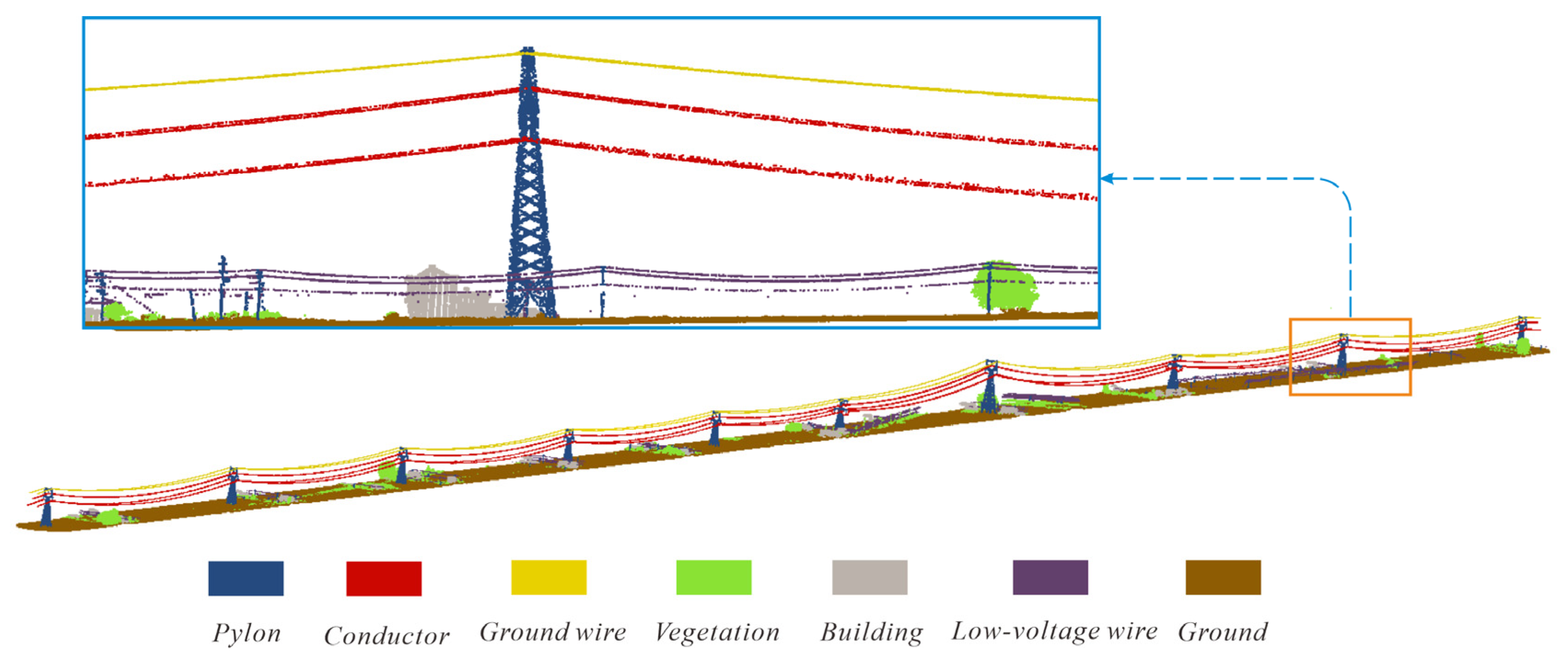
Based on the non-ground point clouds extracted, we manually annotated the categories of each non-ground point cloud. For the current research on semantic segmentation of EHVTLs, all power lines are usually grouped into one category, which is not conducive to accurate semantic segmentation. In this paper, we further divided the power lines into three categories: conductor, ground wire, and low-voltage wire, according to the spatial distribution characteristics and the actual function. In addition, other point cloud data are classified into three categories such as pylon, vegetation, and building. In summary, the point cloud dataset of the 500 kV EHVTL constructed in this paper was divided into six categories: conductor, ground wire, low-voltage wire, pylon, vegetation, and building. The point cloud categories in this dataset contain the common scenes of power line inspections, hence achieving a high applicability and generalization capability. Two adjacent pylons of the EHVTL and the area between the pylons were divided into a section to facilitate network training; thus, the whole dataset was divided into 65 sections, including 54 sections in the training dataset and 11 sections in the test dataset. Figure 6 shows part of the sections in the EHVTL point cloud dataset after manual labeling and the corresponding ground point clouds (shown in brown in Figure 6). Figure 7 shows the statistics of the number of points for each category in the dataset. The characteristics of each category of point clouds in the dataset are briefly described as follows.

(1)

Pylons (shown in blue in Figure 6) are usually divided into two types according to the function: linear pylons and tension-resistant pylons, of which linear pylons generally account for more than 80% of pylons. Tension-resistant pylons are built to anchor conductors, limiting the scope of line faults and facilitating construction and maintenance. The two pylons are not differentiated in the data set due to their similar appearance.

(2)

Ground wires (shown in yellow in Figure 6) are set to protect the conductors from lightning strikes. In 500 kV EHVTLs, two ground wires are usually utilized, and they are erected on top of the entire line, thus placing all the transmission lines within its protection.

(3)

Conductor (shown in red in Figure 6) is a metal wire fixed on the pylon to carry the current. For the 500 kV conductors, it is mostly located below the ground wire and is distributed in two layers.

(4)

Vegetation (shown in green in Figure 6) is mainly arable land, forest, low vegetation beside the road, and so on. Given that most EHVTLs are erected in a field environment with high vegetation coverage, the point cloud of this category still accounts for a relatively large proportion as shown in Figure 6.

(5)

Building (shown in gray in Figure 6) is mainly some residential housing built close to EHVTLs and so on.

(6)

Low-voltage wires (shown in purple in Figure 6) mainly contain low-voltage (<10 kV) transmission lines passing through villages or towns, which account for the lowest proportion in the dataset, as shown in Figure 7.

Figure 6. Point clouds of the EHVTL dataset with labeling.

Figure 6. Point clouds of the EHVTL dataset with labeling.

Figure 7. Point cloud numbers of each category in the EHVTL dataset. (a) Training dataset; (b) test dataset.

Figure 7. Point cloud numbers of each category in the EHVTL dataset. (a) Training dataset; (b) test dataset.

The point cloud numbers of each category in our proposed point cloud dataset based on non-ground point cloud data remain unbalanced. For example, the proportion of the vegetation category is relatively high. However, the point clouds of each category in this dataset cannot be accurately semantically segmented unless deep neural networks with an excellent performance are utilized. Therefore, our dataset can evaluate the semantic segmentation performance of deep neural networks.

4. Network Experiments

The experiments in this paper consisted of two main aspects. We first tested the rationality of the PowerLine-Net architecture and its applicability to the EHVTL point cloud dataset proposed in this paper. At the same time, the segmentation results of PowerLine-Net were compared with those of other mainstream networks. Based on this, the risk point detection on the EHVTL point cloud data was performed using the segmentation results of the PowerLine-Net. Second, we compared the segmentation results of PowerLine-Net with other mainstream networks on the Semantic3D dataset, thus examining the generality of PowerLine-Net.

In the network experiments of this section, we used the Adam optimizer with default parameters. The batch size was 3; the epoch was set to 200; and training stopped when the epoch reached 200. The dependencies included Ubuntu18.04, TensorFlow1.13.1, Python3.7.10, software was Pycharm2021.2. All experiments in this paper used workstations with the same hardware configuration. The CPU model was Intel@Xeon(R) Silver 4114, the memory was 48 GB, and the graphics card was NVIDIA Quadro RTX 4000 with memory of 8 GB. For the result evaluation, the overall accuracy (OA) and mean intersection over union (mIoU) were used to evaluate the overall semantic segmentation results, and the intersection over union (IoU) was used to evaluate the segmentation effect of each category.

4.1. EHVTL Dataset-Based Experiments

4.1.1. Network Architecture Testing

(1)

Efficiency comparison experiments of different encoding strategies

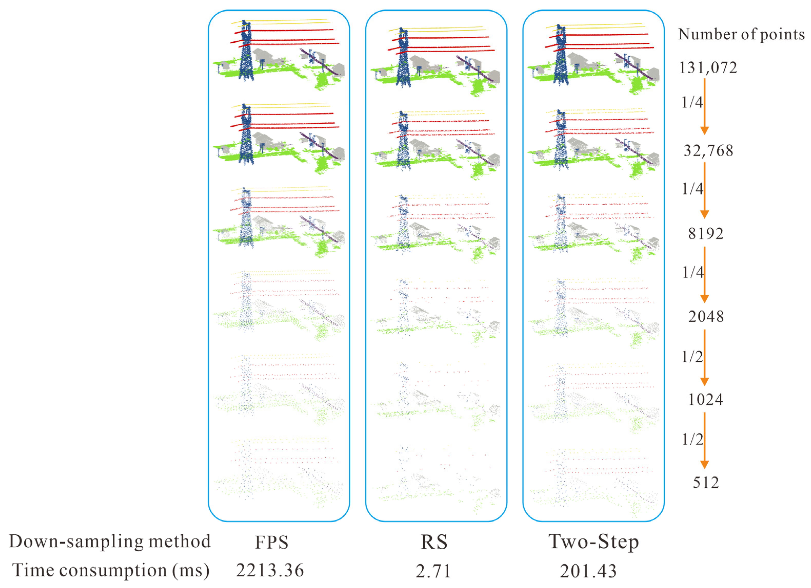
Feature encoding is the core component of deep neural network construction, and its time consumption has a significant effect on the computational efficiency of the network. In order to test the computational efficiency of different feature encoding strategies, we first conducted experiments on three down-sampling methods, including FPS, RS, and TS, with local point clouds selected from the EHVTL dataset. As shown in Figure 8, a central point was randomly selected and the 131,072 points adjacent to it in the EHVTL dataset were collected as the original sample data, which were down-sampled to 512 points by the three above-mentioned methods using five steps (the down-sampling rate of each corresponding step was 1/4, 1/4, 1/4, 1/2, and 1/2). The time consumption for down-sampling was calculated and recorded as 2213.36 ms for FPS, 2.71 ms for RS, and 201.43 ms for TS.

In addition, in order to further compare the computational efficiency of different strategies, we computed the feature encoding using three methods, including TS and LFAPAD-based (TS&LFAPAD) encoding strategy, RS-and-local-feature-aggregation-of-the-points-before-down-sampling-based (RS&LFAPBD) encoding strategy [26], and FPS-and-shared-MLP-based (FPS&MLPs) encoding strategy [19] (note: for convenience, the feature encoding strategies are used here to refer to the corresponding networks). Based on the above randomly selected 131,072 points, the time consumption of the three encoding strategies is shown in

Table 1. Time consumption of different encoding strategies.

Encoding Strategies	Down-Sampling (ms)	Feature Extraction (ms)	Total (ms)
TS&LFAPAD	201.43	519.98	721.41
RS&LFAPBD	2.71	783.59	784.30
FPS&MLPs	2213.36	2478.01	4691.37

, where TS&LFAPAD, RS&LFAPBD, and FPS&MLPs takes 721.52, 784.30, and 4691.37 ms, respectively.

(2)

The comparison of semantic segmentation accuracy for different encoding layer structures

After comparing the efficiency of the encoding strategies, we then compared the semantic segmentation accuracy of the different encoding layer structures. Since the time consumption of the FPS&MLPs encoding strategy is longer than the other two strategies in the above experiments, the efficiency of which is too poor to use, only the TS&LFAPAD and RS&LFAPBD strategies were compared in these experiments.

Based on the EHVTL dataset, we first compared the semantic segmentation accuracy of the two encoding strategies with the same down-sampling rate and encoding layer numbers. Second, we compared the accuracy of different encoding layer numbers with the same down-sampling rate and encoding strategy. Finally, with the same encoding layer numbers and encoding strategy, we compared the accuracy of different down-sampling rates. The quantitative results of the different encoding strategies are shown in Table 2. The specific experimental parameters shown in Table 2 are as follows:

• Comparison of encoding strategies.

Comparison Group #1: Ex. 1 and Ex. 4 are included. The down-sampling rate is [4,4,4,2,2], and the number of down-sampling layers is 5. The encoding strategy for Ex. 1 is TS&LFAPAD and that for Ex. 4 is RS&LFAPBD.

Comparison Group #2: Ex. 2 and Ex. 5 are included. The down-sampling rate is [4,4,4,4,2], and the number of down-sampling layers is 5. The encoding strategy for Ex. 2 is TS&LFAPAD and that for Ex. 5 is RS&LFAPBD.

Comparison Group #3: Ex. 3 and Ex. 6 are included. The down-sampling rate is [4,4,4,4], and the number of down-sampling layers is 4. The encoding strategy for Ex. 3 is TS&LFAPAD and that for Ex. 6 is RS&LFAPBD.

2.

Comparison of the encoding layer numbers

Comparison Group #4: Ex. 1 and Ex. 3 are included. The down-sampling rates are [4,4,4,2,2] and [4,4,4,4], and the encoding strategy is TS&LFAPAD. The number of down-sampling layers for Ex. 1 is 5 and that for Ex. 3 is 4.

Comparison Group #5: Ex. 4 and Ex. 6 are included. The down-sampling rates are [4,4,4,2,2] and [4,4,4,4], and the encoding strategy is RS&LFAPBD. The number of down-sampling layers for Ex. 4 is 5, and that for Ex. 6 is 4.

3.

Comparison of the down-sampling rate

Comparison Group #6: Ex. 1 and Ex. 2 are included. The encoding strategy is TS&LFAPAD, and the number of down-sampling layers is 5. The down-sampling rate for Ex.1 is [4,4,4,2,2] and that for Ex. 2 is [4,4,4,4,2].

Comparison Group #7: Ex. 4 and Ex. 5 are included. The encoding strategy is RS&LFAPBD, and the number of down-sampling layers is 5. The down-sampling rate for Ex.4 is [4,4,4,2,2] and that for Ex. 5 is [4,4,4,4,2].

Table 2. Quantitative results of the EHVTL dataset for different encoding layer structures (%).

Encoding Layer Structure				OA	IoU
No.	Number of Layers	Encoding Strategy	Down-Sampling Rate		mIoU	#1	#2	#3	#4	#5	#6
Ex. 1	5	TS&LFAPAD	[4,4,4,2,2]	98.60	91.45	97.61	88.88	98.40	99.33	95.15	69.35
Ex. 2	5	TS&LFAPAD	[4,4,4,4,2]	97.06	88.13	95.54	89.03	98.97	99.01	92.08	54.12
Ex. 3	4	TS&LFAPAD	[4,4,4,4]	97.11	85.11	95.75	90.21	97.48	98.51	89.94	38.74
Ex. 4	5	RS&LFAPBD	[4,4,4,2,2]	96.33	82.25	94.25	79.61	91.45	98.76	91.04	37.10
Ex. 5	5	RS&LFAPBD	[4,4,4,4,2]	96.32	82.18	95.12	85.98	87.91	96.24	92.21	35.59
Ex. 6	4	RS&LFAPBD	[4,4,4,4]	90.32	59.50	91.32	77.11	11.54	76.91	84.11	15.99

Notes: The category labels correspond to {#1: vegetation, #2: pylon, #3: ground wire, #4: l conductor, #5: building, #6: low-voltage wire}. The numbers inside brackets ([ ]) in the table indicate the ratio of points before and after down-sampling under each layer.

Table 2. Quantitative results of the EHVTL dataset for different encoding layer structures (%).

Encoding Layer Structure				OA	IoU
No.	Number of Layers	Encoding Strategy	Down-Sampling Rate		mIoU	#1	#2	#3	#4	#5	#6
Ex. 1	5	TS&LFAPAD	[4,4,4,2,2]	98.60	91.45	97.61	88.88	98.40	99.33	95.15	69.35
Ex. 2	5	TS&LFAPAD	[4,4,4,4,2]	97.06	88.13	95.54	89.03	98.97	99.01	92.08	54.12
Ex. 3	4	TS&LFAPAD	[4,4,4,4]	97.11	85.11	95.75	90.21	97.48	98.51	89.94	38.74
Ex. 4	5	RS&LFAPBD	[4,4,4,2,2]	96.33	82.25	94.25	79.61	91.45	98.76	91.04	37.10
Ex. 5	5	RS&LFAPBD	[4,4,4,4,2]	96.32	82.18	95.12	85.98	87.91	96.24	92.21	35.59
Ex. 6	4	RS&LFAPBD	[4,4,4,4]	90.32	59.50	91.32	77.11	11.54	76.91	84.11	15.99

Notes: The category labels correspond to {#1: vegetation, #2: pylon, #3: ground wire, #4: l conductor, #5: building, #6: low-voltage wire}. The numbers inside brackets ([ ]) in the table indicate the ratio of points before and after down-sampling under each layer.

4.1.2. Comparison of Different Deep Neural Networks

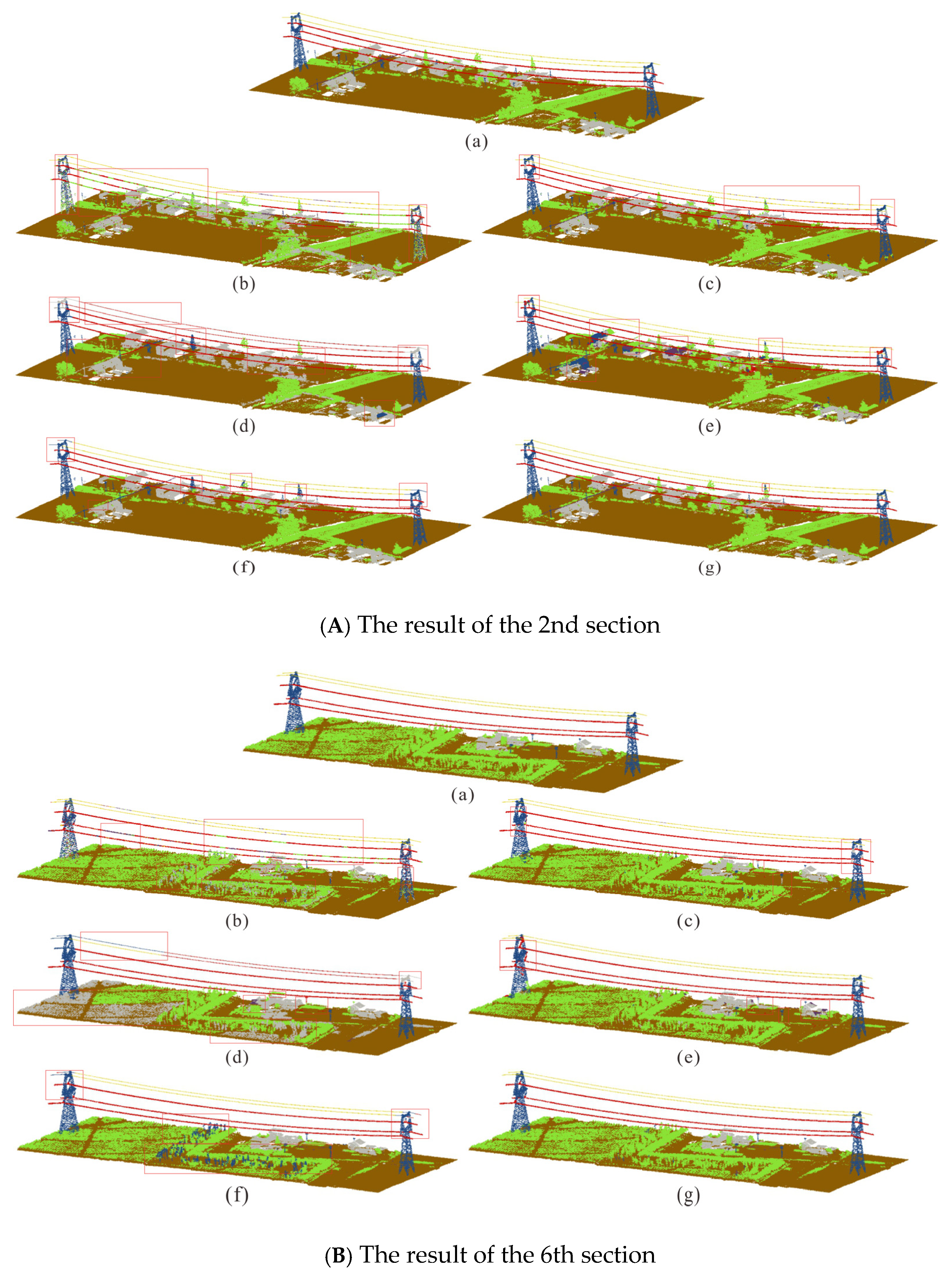
In this part, the semantic segmentation of EHVTL point cloud data is realized based on the RandLA-Net, KPConv, SPG, PointNet++, PointCNN, and PowerLine-Net proposed in this paper. The quantitative results of semantic segmentation are shown in

Table 3. Quantitative results of the EHVTL dataset for different networks.

Networks	Time	OA	IoU
			mIoU	#1	#2	#3	#4	#5	#6
PointCNN [20]	660	85.03	49.44	80.70	39.12	51.93	40.83	76.95	7.09
KPConv [21]	566	96.09	68.62	96.96	65.62	56.92	77.84	94.96	19.43
SPG [22]	720	79.62	49.35	71.04	58.54	32.17	70.71	61.80	1.84
PointNet++ [23]	1077	77.25	53.04	75.26	42.43	77.66	77.66	28.86	1.06
RandLA-Net [26]	593	96.33	82.25	94.25	79.61	91.45	98.76	91.04	37.10
PowerLine-Net (Ours)	510	98.60	91.45	97.61	88.88	98.40	99.33	95.15	69.35

Notes: The category labels correspond to {#1: vegetation, #2: pylon, #3: ground wire, #4: l conductor, #5: building, #6: low-voltage wire; the unit of training time is $s/epoch$; bold: optimal results}.

. Moreover, in order to visualize the semantic segmentation effect of different networks, we present the results of the six networks (shown in Figure 9). In addition, two sections in the test dataset containing different features are magnified. The red squares in the figure represent the areas where the segmentation results of the point clouds are incorrect.

As shown in Table 3, PowerLine-Net has been greatly improved compared with the above five networks. The IoU of pylons is improved by 49.76%, 23.26%, 30.34%, 46.45%, and 9.27% (9.27–49.76%); the IoU of the ground line is improved by 46.47%, 41.48%, 66.23 %, 20.74%, and 6.95% (6.95%–66.23 %); the IoU of conductor lines is improved by 58.5%, 21.49%, 28.62%, 21.67%, and 0.57% (0.57–58.5%); and the IoU of the low-voltage wire is improved by 62.26%, 49.92%, 67.51%, 68.29%, and 32.25% (32.25–68.29%), respectively.

4.1.3. Risk Point Detection Based on Semantic Segmentation Results

In order to protect the safety of life and property, EHVTLs should be designed with a high span when crossing forests or human living areas and should meet the safety distance requirements. The risk point detection (i.e., safety distance detection) of the EHVTL is mainly through the calculation of the safety distances between the objects, including vegetation, ground and buildings, and conductors (shown in Figure 10), and risk points that do not meet the requirements are then accurately located based on the safety distance rules (shown in

Table 4. Safety distance rules of the 500 kV EHVTL.

Objects	Crossover	Vegetation	Building	Ground
safety distance (m)	6	7	9	11

Notes: Safety distance rules are based on the “Overhead Transmission Line Operation Regulations” (DL/T 741-2010).

) to promptly remove the safety hazards. Since the actual task of the EHVTL inspection is huge, the semantic segmentation results based on deep learning for risk point detection should be applied to improve the inspection efficiency. In this paper, we used the semantic segmentation results of the point clouds of the EHVTL based on the PowerLine-Net network to realize the risk point detection.

After detection, a risk point is found in the point cloud data. Under the constructed local coordinate system, the point cloud data of the EHVTL section where the risk point is located are shown in Figure 11. In Figure 11, the risk point is marked in pink, and its information is shown in

Table 5. Information about the risk point (m).

ID	Section No.	Span	Object	Horizontal Distance	Vertical Distance	Clearance Distance	Safety Distance
1	12–13	396.19	vegetation	3.14	5.10	5.99	7

. Compared with traditional inspections based on manual operations, this method based on the PowerLine-Net not only obtains accurate risk point information but also significantly improves the efficiency and reduces labor costs.

4.2. Experiments on the Semantic3D Dataset

In order to validate the generalization ability and segmentation accuracy of the PowerLine-Net, we realized the semantic segmentation of the point clouds based on the Semantic3D dataset [34]. It is a generic dataset for urban scenes with over 1.2 billion sampling points, each containing coordinate, color, and intensity information. Its point cloud data are divided into eight categories, with scenes mainly including churches, streets, railway tracks, squares, villages, soccer fields, castles, and so on. In this paper, we implemented the training of the PowerLine-Net network on Semantic3D and conducted semantic segmentation using the reduced-8 test dataset of the Semantic3D. The qualitative results are shown in Figure 12. In order to compare accuracy, we realized semantic segmentation based on the same dataset with five networks, including PointNet++, PointCNN, SPG, KPConv, and RandLA-Net. In

Table 6. Quantitative results on the Semantic3D(reduced-8) test dataset for different networks (%).

Network Name	Time	OA	IoU
			mIoU	Man-Made Terrain	Natural Terrain	High Vegetation	Low Vegetation	Buildings	Hard Scape	Scanning Artefacts	Cars
PointCNN [20]	1430	92.2	71.8	89.1	82.4	85.5	51.5	94.1	38.4	59.3	68.7
KPConv [21]	600	92.9	74.6	90.9	82.2	84.2	47.9	94.9	40.0	77.3	79.7
SPG [22]	3000	94.0	73.2	97.4	92.6	87.9	44.0	93.2	31.0	63.5	76.2
PointNet++ [23]	3572	92.0	62.4	96.3	92.1	84.4	15.4	93.3	29.2	18.3	70.4
RandLA-Net [26]	670	94.8	77.4	95.6	91.4	86.6	51.5	95.7	51.5	69.8	76.8
PowerLine-Net	594	93.6	77.2	94.4	88.5	84.9	53.8	94.1	52.2	72.4	76.9

Notes: Time demotes the test time, unit: s; bold: optimal results.

, we list the semantic segmentation accuracy of the reduced-8 test dataset with different networks.

As shown in Table 6, The PowerLine-Net improved (IoU) by 2.3%, 5.9%, 9.8%, 38.4%, and 2.3% for the low vegetation category and 13.8%, 12.2%, 21.2%, 23.0%, and 0.7% for the hardscape category compared to other networks.

5. Discussions

In this paper, we conducted data experiments for the PowerLine-Net network based on the EHVTL dataset and the Semantic3D dataset. The results of the above experiments are discussed below.

5.1. Experiments for the PowerLine-Net Network Based on the EHVTL Dataset

5.1.1. Comparison Analysis of Network Architecture

A total of 131,072 points in the EHVTL dataset were selected to contrast the efficiency of the FPS, RS, and TS methods. These points were then used to compare the efficiency of the TS&LFAPAD, RS&LFAPBD, and FPS&MLPS strategies. The comparison results are shown in Figure 8 and Table 1. FPS (2213.36 ms) consumes more time than RS (2.71 ms) and TS (201.43 ms) at the same down-sampling rate. The total computation time of the TS&LFAPAD and RS&LFAPBD strategies are similar, both in the range of 700–800 ms; the FPS&MLPS takes the longest time (4691.37 ms), which is much longer than the other two encoding strategies. The FPS&MLPs strategy is considerably inefficient for EHVTL data. At the same time, the TS&LFAPAD and RS&LFAPBD strategies have a comparable computational efficiency and can preserve the overall geometric features of different objects in the sample data (as shown in Figure 8), which can meet the needs for semantic segmentation on the EHVTL point cloud data.

Based on the TS&LFAPAD and RS&LFAPBD strategies, we contrasted the semantic segmentation accuracy on the EHVTL dataset for the deep neural networks with different down-sampling rates and different numbers of down-sampling layers. According to the results of Comparison Groups #1, #2, and #3, with the same down-sampling rate and number of down-sampling layers, the networks with the TS&LFAPAD strategy have higher mIoU and OA scores than the networks with the RS&LFAPBD strategy, indicating that the TS&LFAPAD strategy is more suitable for the semantic segmentation of the EHVTL point cloud data. According to the results of Comparison Groups #4 and #5, with the same down-sampling rate and encoding strategy, the networks with five down-sampling layers have higher mIoU and OA scores than the network with four down-sampling layers, proving that the use of five down-sampling layers with the TS&LFAPAD strategy is more conducive to segmentation on the EHVTL point cloud data. According to the results of Comparison Groups #6 and #7, with the same number of down-sampling layers and encoding strategy, the networks with the down-sampling rate of [4,4,4,2,2] have higher mIoU and OA scores than the network with the down-sampling rate of [4,4,4,4,2], proving that the use of a down-sampling rate of [4,4,4,2,2] with the TS&LFAPAD strategy is more conducive to segmentation on the EHVTL point cloud data. In summary, for PowerLine-Net, the encoding layer structures using the five encoding layers, a [4,4,4,2,2] down-sampling rate and TS&LFAPAD encoding strategy have a higher computational efficiency and segmentation accuracy than other encoding layer structures in semantic segmentation on EHVTL point cloud data.

5.1.2. Comparison Analysis of the PowerLine-Net and Mainstream Networks

The PowerLine-Net was compared with the current mainstream point-based deep neural networks, including PointCNN, KPConv, SPG, PointNet++, and RandLA-Net, based on the EHVTL dataset. The quantitative results of various networks for semantic segmentation are shown in Table 3. From the quantitative results, the accuracy of the PowerLine-Net network is evidently higher than the other five networks in all categories. In particular, for categories with small-quantity point clouds, PowerLine-Net has been greatly improved compared with the above five networks. In summary, the PowerLine-Net is better than RandLA-Net, KPConv, SPG, PointNet++, and PointCNN, especially regarding the category with small-quantity point clouds, thus proving the superiority of PowerLine-Net in the semantic segmentation on EHVTL point clouds.

5.1.3. Application of Risk Point Detection on EHVTL Point Clouds

According to the safety distance criterion shown in Table 4, the risk point detection on the EHVTL point clouds is achieved based on the semantic segmentation results of PowerLine-Net, and the results of detection are shown in Figure 11. A risk point is marked in pink, and, besides that, the further acquisition of risk point information is achieved, which is shown in Table 5, including the location, type, and safety distance. The risk point appears in the 12th–13th section, with a spacing of 396.19 m. The main reason for the risk is the close distance between the vegetation and the conductor, where the horizontal distance is 3.14 m and the vertical distance is 5.10 m. This illustrates the practicality of the PowerLine-Net network for the risk point detection of actual EHVTL inspections.

5.2. Experiments for the PowerLine-Net Network Based on the Semantic3D Dataset

We compared the semantic segmentation accuracy of PowerLine-Net with mainstream networks, including PointCNN, KPConv, SPG, PointNet++, and RandLA-Net, on the Semantic3D dataset. The quantitative results of the above six networks are shown in Table 6. In terms of the IoU, PowerLine-Net is close to RandLA-Net and outperforms the other four mainstream networks. In particular, the IoUs of PowerLine-Net are better than the other five networks in the categories of low vegetation and hard scape (e.g., street lights, signs, and other public facilities), which have fewer point clouds and are difficult to segment. This illustrates that the PowerLine-Net can perform high-precision semantic segmentation on the categories with small-quantity point clouds while ensuring a high semantic segmentation accuracy on categories with large-quantity point clouds.

6. Conclusions

In this paper, in order to achieve semantic segmentation of the EHVTL point cloud data based on deep neural networks, we proposed the PowerLine-Net based on the TS method and the LFAPAD. Furthermore, in order to compare the semantic segmentation effect of PowerLine-Net with other networks, an EHVTL point cloud dataset was constructed, which consists of six categories: conductor, ground wire, low-voltage wire, pylon, vegetation, and building. The performance of the PowerLine-Net network was then tested based on the EHVTL point cloud dataset and the Semantic3D dataset, and the specific conclusions are as follows.

From the experimental results of the EHVTL point clouds dataset, we found that (1) PowerLine-Net with five encoding layers, a [4,4,4,4,2,2] down-sampling rate, and a TS&LFASP encoding strategy have a better efficiency and computational accuracy than other encoding layer structures; (2) compared with mainstream deep neural networks, including PointCNN, KPConv, SPG, PointNet++, and RandLA-Net, PowerLine-Net performs well in all categories, especially in the three categories of conductor, ground wire, and low-voltage wire, where its segmentation accuracy is significantly better than other networks; (3) the semantic segmentation results of the PowerLine-Net can be used to detect risk points on the EHVTL point clouds, thus demonstrating the important value of the network in practical work.

From the experimental results of the Semantic3D dataset, the PowerLine-Net network has a higher segmentation accuracy compared with the current mainstream deep neural networks, especially for categories with small-quantity point clouds. This finding indicates that the network can effectively reduce the impact of the unbalanced number of points of different categories on the semantic segmentation results, and is suitable for the semantic segmentation of large-field point cloud datasets.

In summary, PowerLine-Net has an efficient and accurate semantic segmentation capability for large-scene point clouds and provides a powerful method for supporting transmission line inspection point cloud data processing.

References

1. Fitiwi, D.Z.; De Cuadra, F.; Olmos, L.; Rivier, M. A new approach of clustering operational states for power network expansion planning problems dealing with RES (renewable energy source) generation operational variability and uncertainty. Energy 2015, 90, 1360–1376. [Google Scholar] [CrossRef]
2. Ye, L.; Liu, Q.; Hu, Q.W. Research of Power Line Fitting and Extraction Techniques Based on Lidar Point Cloud Data. Geomat. Spat. Inf. Technol. 2010, 33, 30–34. [Google Scholar]
3. Yu, J.; Mu, C.; Feng, Y.M.; Dou, Y.J. Powerlines Extraction Techniques from Airborne LiDAR Data. Geomat. Inf. Sci. Wuhan Univ. 2011, 36, 1275–1279. [Google Scholar]
4. Zhang, W.M.; Yan, G.J.; Li, Q.Z.; Zhao, W. 3D Power Line Reconstruction by Epipolar Constraint in Helicopter Power Line Inspection System. J. Beijing Norm. Univ. 2006, 42, 629–632. [Google Scholar]
5. Li, X.; Wen, C.C.; Cao, Q.M.; Du, Y.L.; Fang, Y. A novel semi-supervised method for airborne LiDAR point cloud classification. ISPRS J. Photogramm. Remote Sens. 2021, 180, 117–129. [Google Scholar] [CrossRef]
6. Hooper, B. Vegetation Management Takes to the Air. Transm. Distrib. World 2003, 55, 78–85. [Google Scholar]
7. Ahmad, J.; Malik, A.; Xia, L.K.; Ashikin, N. Vegetation encroachment monitoring for transmission lines right-of-ways: A survey. Electr. Power Syst. Res. 2013, 95, 339–352. [Google Scholar] [CrossRef]
8. Xu, Z.J.; Wang, Z.Z.; Yang, F. Airborne Laser Radar Measurement Technology and the Engineering Application Practice; Wuhan University Press: Wuhan, China, 2009. [Google Scholar]
9. McLaughlin, R.A. Extracting Transmission Lines From Airborne LIDAR Data. IEEE Geosci. Remote Sens. Lett. 2006, 3, 222–226. [Google Scholar] [CrossRef]
10. Zhou, R.Q.; Xu, Z.H.; Peng, C.G.; Zhang, F.; Jiang, W.S. A Joint Boost-based classification method of high voltage transmission corridor from airborne LiDAR point cloud. Sci. Surv. Mapp. 2019, 44, 21–27. [Google Scholar]
11. Zhang, J.Y.; Zhao, X.L.; Chen, Z.; Lu, Z.C. A review of deep learning-based semantic segmentation for point cloud. IEEE Access 2019, 7, 179118–179133. [Google Scholar] [CrossRef]
12. Shi, C.H.; Li, J.; Gong, J.H.; Yang, B.H.; Zhang, G.Y. An improved lightweight deep neural network with knowledge distillation for local feature extraction and visual localization using images and LiDAR point clouds. ISPRS J. Photogramm. Remote Sens. 2022, 184, 177–188. [Google Scholar] [CrossRef]
13. Graham, B.; Engelcke, M.; van der Maaten, L. 3D semantic segmentation with submanifold sparse convolutional networks. In Proceedings of the 2018 IEEE/CVF Conference on Computer Vision and Pattern Recognition (CVPR), Salt Lake City, UT, USA, 18–23 June 2018; IEEE: Piscataway, NJ, USA, 2018; Volume 1, pp. 9224–9232. [Google Scholar]
14. Meng, H.Y.; Gao, L.; Lai, Y.K.; Manocha, D. VV-net: Voxel VAE Net with group convolutions for point cloud segmentation. In Proceedings of the 2019 IEEE/CVF International Conference on Computer Vision (ICCV), Seoul, Republic of Korea, 27 October–2 November 2019; IEEE: Piscataway, NJ, USA, 2019; Volume 1, pp. 8499–8507. [Google Scholar]
15. Chen, X.Z.; Ma, H.M.; Wan, J.; Li, B.; Xia, T. Multi-view 3D Object Detection Network for Autonomous Driving. In Proceedings of the 2017 IEEE Conference on Computer Vision and Pattern Recognition (CVPR), Honolulu, HI, USA, 21–26 July 2017; IEEE: Piscataway, NJ, USA, 2017; Volume 1, pp. 6526–6534. [Google Scholar]
16. Yang, B.; Luo, W.; Urtasun, R. PIXOR: Real-time 3D object detection from point clouds. In Proceedings of the 2018 IEEE/CVF Conference on Computer Vision and Pattern Recognition, Salt Lake City, UT, USA, 18–23 June 2018; IEEE: Piscataway, NJ, USA, 2018; Volume 1, pp. 7652–7660. [Google Scholar]
17. Zhang, R.; Li, G.Y.; Li, M.L.; Wang, L. Fusion of images and point clouds for the semantic segmentation of large-scale 3D scenes based on deep learning. ISPRS J. Photogramm. Remote Sens. 2018, 143, 85–96. [Google Scholar] [CrossRef]
18. Lang, A.H.; Vora, S.; Caesar, H.; Zhou, L.; Beijbom, O. PointPillars: Fast encoders for object detection from point clouds. In Proceedings of the 2019 IEEE/CVF Conference on Computer Vision and Pattern Recognition (CVPR), Long Beach, CA, USA, 15–20 June 2019; IEEE: Piscataway, NJ, USA, 2019; Volume 1, pp. 12689–12697. [Google Scholar]
19. Qi, C.R.; Su, H.; Mo, K.; Guibas, L.J. PointNet: Deep Learning on Point Sets for 3D Classification and Segmentation. In Proceedings of the 2017 IEEE Conference on Computer Vision and Pattern Recognition (CVPR), Honolulu, HI, USA, 21–26 July 2017; IEEE: Piscataway, NJ, USA, 2017; Volume 1, pp. 77–85. [Google Scholar]
20. Li, Y.Y.; Bu, R.; Sun, M.C.; Wu, W.; Di, X.H.; Chen, B.Q. Pointcnn: Convolution on x-transformed points. Adv. Neural Inf. Process. Syst. 2018, 31, 828–838. [Google Scholar]
21. Thomas, H.; Qi, C.R.; Deschaud, J.E.; Marcotegui, B.; Goulette, F.; Guibas, L.J. Kpconv: Flexible and deformable convolution for point clouds. In Proceedings of the 2019 IEEE/CVF international conference on computer vision (ICCV), Seoul, Republic of Korea, 27 October–2 November 2019; IEEE: Piscataway, NJ, USA, 2019; Volume 1, pp. 6411–6420. [Google Scholar]
22. Landrieu, L.; Simonovsky, M. Large-scale point cloud semantic segmentation with superpoint graphs. In Proceedings of the 2018 IEEE/CVF Conference on Computer Vision and Pattern Recognition, Salt Lake City, UT, USA, 18–23 June 2018; IEEE: Piscataway, NJ, USA, 2018; Volume 1, pp. 4558–4567. [Google Scholar]
23. Qi, C.R.; Yi, L.; Su, H.; Guibas, L.J. PointNet++: Deep hierarchical feature learning on point sets in a metric space. In Proceedings of the 31st International Conference on Neural Information Processing Systems, Red Hook, NY, USA, 4 December 2017; Curran Associates Inc.: Red Hook, NY, USA, 2017; Volume 1, pp. 5105–5114. [Google Scholar]
24. Lai, X.; Liu, J.H.; Jiang, L.; Wang, L.W.; Zhao, H.S.; Liu, S.; Qi, X.J.; Jia, J.Y. Stratified transformer for 3d point cloud segmentation. In Proceedings of the 2022 IEEE/CVF Conference on Computer Vision and Pattern Recognition, New Orleans, LA, USA, 18–24 June 2022; pp. 8500–8509. [Google Scholar]
25. Qian, G.C.; Li, Y.C.; Peng, H.W.; Mai, J.J.; Hammoud, H.; Elhoseiny, M.; Ghanem, B. Pointnext: Revisiting pointnet++ with improved training and scaling strategies. Adv. Neural Inf. Process. Syst. 2022, 35, 23192–23204. [Google Scholar]
26. Hu, Q.Y.; Yang, B.; Xie, L.H.; Rosa, S.; Guo, Y.L.; Wang, Z.H.; Trigoni, N.; Markham, A. RandLA-Net: Efficient Semantic Segmentation of Large-Scale Point Clouds. In Proceedings of the 2020 IEEE/CVF Conference on Computer Vision and Pattern Recognition (CVPR), Seattle, WA, USA, 13–19 June 2020; IEEE: Piscataway, NJ, USA, 2020; Volume 1, pp. 11105–11114. [Google Scholar]
27. Fan, S.Q.; Dong, Q.L.; Zhu, F.H.; Lv, Y.S.; Ye, P.J.; Wang, F.Y. SCF-Net: Learning spatial contextual features for large-scale point cloud segmentation. In Proceedings of the 2021 IEEE/CVF Conference on Computer Vision and Pattern Recognition, Nashville, TN, USA, 20–25 June 2021; IEEE: Piscataway, NJ, USA, 2021; Volume 1, pp. 14504–14513. [Google Scholar]
28. Deng, S.; Dong, Q. GA-NET: Global attention network for point cloud semantic segmentation. IEEE Signal Process. Lett. 2021, 28, 1300–1304. [Google Scholar] [CrossRef]
29. Chen, Z.Y.; Peng, S.W.; Zhu, H.D.; Zhang, C.T.; Xi, X.H. LiDAR Point Cloud Classification of Transmission Corridor based on Sample Weighted-PointNet++. Remote Sens. Technol. Appl. 2021, 36, 1299–1305. [Google Scholar]
30. Sheshappanavar, S.V.; Kambhamettu, C. A novel local geometry capture in pointnet++ for 3D classification. In Proceedings of the 2020 IEEE/CVF Conference on Computer Vision and Pattern Recognition Workshops, Seattle, WA, USA, 14–19 June 2020; IEEE: Piscataway, NJ, USA, 2020; Volume 1, pp. 262–263. [Google Scholar]
31. Chen, Y.; Liu, G.L.; Xu, Y.M.; Pan, P.; Xing, Y. PointNet++ network architecture with individual point level and global features on centroid for ALS point cloud classification. Remote Sens. 2021, 13, 472. [Google Scholar] [CrossRef]
32. Vishwanath, K.V.; Gupta, D.; Vahdat, A.; Yocum, K. Modelnet: Towards a datacenter emulation environment. In Proceedings of the 2009 IEEE Ninth International Conference on Peer-to-Peer Computing, Seattle, WA, USA, 9–11 September 2009; Volume 1, pp. 81–82. [Google Scholar]
33. Dai, A.; Chang, A.X.; Savva, M.; Halber, M.; Funkhouser, T.; Nießner, M. ScanNet: Richly-annotated 3D reconstructions of indoor scenes. In Proceedings of the 2017 IEEE Conference on Computer Vision and Pattern Recognition (CVPR), Honolulu, HI, USA, 21–26 July 2017; IEEE: Piscataway, NJ, USA, 2017; Volume 1, pp. 2432–2443. [Google Scholar]
34. Hackel, T.; Savinov, N.; Ladicky, L.; Wegner, J.D.; Schindler, K.; Pollefeys, M. Semantic3d.net: A new large-scale point cloud classification benchmark. ISPRS Ann. Photogramm. Remote Sens. Spat. Inf. Sci. 2017, 41, 91–98. [Google Scholar] [CrossRef]
35. Geiger, A.; Lenz, P.; Urtasun, R. Are we ready for autonomous driving? The KITTI vision benchmark suite. In Proceedings of the 2012 IEEE Conference on Computer Vision and Pattern Recognition (CVPR), Providence, RI, USA, 16–21 June 2012; IEEE: Piscataway, NJ, USA, 2012; Volume 1, pp. 3354–3361. [Google Scholar]
36. Dong, Z.; Liang, F.; Yang, B.; Xu, Y.; Stilla, U. Registration of large-scale terrestrial laser scanner point clouds: A review and benchmark. ISPRS J. Photogramm. Remote Sens. 2020, 163, 327–342. [Google Scholar] [CrossRef]
37. Yang, B.S.; Han, X.; Dong, Z. Point Cloud Benchmark Dataset WHU-TIS and WHU-MLS for Deep Learning. J. Remote Sens. 2021, 25, 231–240. [Google Scholar]
38. Jiang, L.X.; Cai, Z.H.; Wang, D.H.; Jiang, S.W. Survey of improving k-nearest-neighbor for classification. In Proceedings of the 2007 IEEE Fourth International Conference on Fuzzy Systems and Knowledge Discovery (FSKD), Haikou, China, 24–27 August 2007; IEEE: Piscataway, NJ, USA, 2007; Volume 1, pp. 679–683. [Google Scholar]
39. Vosselman, G. Slope based filtering of laser altimetry data. Int. Arch. Photogramm. Remote Sens. 2000, 33, 935–942. [Google Scholar]
40. Zhang, K.Q.; Chen, S.C.; Whitman, D.; Shyu, M.L.; Yan, J.H.; Zhang, C.C. A progressive morphological filter for removing nonground measurements from airborne LIDAR data. IEEE Trans. Geosci. Remote Sens. 2003, 41, 872–882. [Google Scholar] [CrossRef]
41. Axelsson, P. DEM Generation from Laser scanner Data Using Adaptive TIN Model. Int. Arch. Photogramm. Remote Sens. 2000, 23, 110–117. [Google Scholar]
42. Zhang, J.X.; Lin, X.G. Filtering airborne LiDAR data by embedding smoothness-constrained segmentation in progressive TIN densification. ISPRS J. Photogramm. Remote Sens. 2013, 81, 44–59. [Google Scholar] [CrossRef]
43. Zhang, W.M.; Qi, J.B.; Wan, P.; Wang, H.T.; Xie, D.H.; Wang, X.Y.; Yan, G.J. An easy-to-use airborne Li-DAR data filtering method based on cloth simulation. Remote Sens. 2016, 8, 501. [Google Scholar] [CrossRef]
Figure 1. Network structure (“local feature aggregation” indicates local feature aggregation of point clouds after down-sampling in each layer of the model).
Remotesensing 15 02371 g001
Figure 2. The module of LFAPAD (yellow dots indicate the point of (i − 1)th layer, red dots indicate the point ( p i ; p i m p i ) of ith layer, and blue dot indicates the mth point ( a i , m ) in the point cloud of the ith layer;   f i , m denotes nearest neighbor point features; r i , m denotes the relative spatial positional information between points; f ^ i , m denotes the local nearest neighbor feature; ⨀ denotes Hadamard product; s i , m denotes the attention score).
Remotesensing 15 02371 g002
Figure 3. Schematic of feature decoding in l th layer. ( N l denotes the number of point clouds in the lth encoding layer, 3 denotes the coordinate feature dimensions (x, y, z), and C l denotes the feature dimensions other than coordinates.)
Remotesensing 15 02371 g003
Figure 4. The network structure of the PowerLine-Net. (“RS” denotes random down-sampling on point clouds; “FPS” denotes farthest point down-sampling on point clouds; “FP” indicates feature propagation. The sizes of MLP on C i , C ^ i (i = 1, 2, … 5) are [32,32,64] for C 0 to C 1 , [64,64,128] for C 1 to C 2 , [128,128,256] for C 2 to C 3 , [256,256,512] for C 3 to C 4 , [512,512,1024] for C 4 to C 5 , [1024,1024,512] for C 5 to C ^ 5 , [512,512] for C ^ 5 to C ^ 4 , [512,256] for C ^ 4 to C ^ 3 , [256,256] for C ^ 3 to C ^ 2 , [256,128] for C ^ 2 to C ^ 1 , and [128,128,128] for C ^ 1 to C ^ 0 , respectively. The activation function is ReLU.)
Remotesensing 15 02371 g004
Figure 5. Parts of original point cloud data.
Remotesensing 15 02371 g005
Figure 8. Comparison of three down-sampling methods.
Remotesensing 15 02371 g008
Figure 9. Qualitative results of the EHVTL dataset for different networks. (a) Ground truth; (b) PointCNN; (c) KPConv; (d) SPG; (e) PointNet++; (f) RandLA-Net; (g) PowerLine-Net.
Remotesensing 15 02371 g009
Figure 10. Schematic of the safety distances.
Remotesensing 15 02371 g010
Figure 11. Schematic of EHVTL cross-sectional point cloud data with risk points. (a) Top view of the EHVTL section; (b) front view of the EHVTL section; (c) side view of the EHVTL section; the coordinates of the risk point (x, y, z): (227.75, 57.91, 18.73); the coordinates of the power line risk point (x, y, z): (227.75, 54.77, 23.83). The pink points: risk points; the pink triangle: the location of risk points.
Remotesensing 15 02371 g011
Figure 12. Qualitative results on the Semantic3D(reduced-8) test dataset for the PowerLine-Net.
Remotesensing 15 02371 g012