Multi-Dimensional Spread Target Detection with Across Range-Doppler Unit Phenomenon Based on Generalized Radon-Fourier Transform

Abstract

Severe phenomena of across range-Doppler unit (ARDU) and decoherence occur when radar detects high-speed and high-maneuvering targets, causing degradation in detection performance of traditional FFT radar detection methods. The improvement in radar resolution causes a multi-dimensional spread phenomenon, where different scattering centers of the target are distributed on different range units, along with motion parameters such as velocity and acceleration. Unfortunately, current radar detection methods focus solely on range spread targets and cannot handle multi-dimensional spread, leading to a significant decline in detection performance. To overcome this problem, this paper proposes several methods to achieve high detection performance for multi-dimensional spread target detection with ARDU phenomenon. Firstly, the generalized likelihood ratio test (GLRT) is derived, and the energy integration generalized Rayleigh Fourier transform (EI-GRFT) is introduced to improve the detection performance of range spread cross-unit targets. Additionally, the double-threshold based hybrid GRFT (DT-HGRFT) is presented as an enhancement of EI-GRFT, enabling long-time integration along slow time and integration among multiple scatters by using HGRFT and multi-dimensional sliding double-threshold detection, respectively. Furthermore, a method for joint detections of multiple DT-HGRFTs is provided to handle the case where the number of scattering centers of multi-dimensional spread targets is unknown. Finally, a detailed theoretical analysis of the performance of the proposed method is presented, along with extensive simulations and practical experiments to demonstrate the effectiveness of the proposed methods.

1. Introduction

In accordance with the radar equation, the signal to noise ratio (SNR) and detection performance can be effectively improved by integrating over a long period along the slow time dimension [1,2]. For instance, the moving target detector (MTD) [3] utilizes Fast Fourier Transform (FFT) to accumulate multiple pulses, concentrating the echo energy on the same range-Doppler unit, thereby enabling multi-pulse coherent integration while distinguishing different speed targets. However, when attempting to achieve long integration time for high speed and maneuverability targets, the phenomenon of ARDU, i.e., across-range unit (ARU) and across-Doppler unit (ADU), is prone to manifest in the echo. In such cases, the echo energy integrated by conventional methods becomes dispersed over multiple range-Doppler units, thereby significantly impairing the detection performance. Moreover, when the scattering characteristics of the target change with angle [3], the amplitude and phase of the echo fluctuate, resulting in the occurrence of the echo decoherence phenomenon which further deteriorates the detection performance.

To solve the problem of ARDU, Radon-Fourier Transform (RFT) and GRFT are proposed in [4,5,6,7,8,9], which can overcome the ARDU phenomenon and achieve the optimal integration of non-undulating targets through parametric modeling and envelope phase joint compensation. For the problem of target echo fluctuation, many fluctuation models are established, such as the Swerling model [10] and the moderate fluctuation model [11,12]. Besides, some detectors are proposed, such as the moderate fluctuation optimal detector and the suboptimal hybrid integration detector (HID). Unfortunately, the above methods are mainly aimed at low-resolution radar.

Compared to low-resolution radar, high-resolution radar significantly enhances range resolution while also offering high measurement accuracy, strong echo coherence, and extensive target structure information. which is widely used in remote sensing [13,14,15,16,17,18,19,20], space surveillance [21,22,23,24,25,26] and astronomical observation [27,28,29,30,31,32,33,34,35]. However, the ARDU phenomenon in high-resolution radar will become more serious. Furthermore, high-resolution radar detection poses a challenge of target with multi-dimensional spread. In situations where the range resolution of the high-resolution radar is smaller than the target size, the target echo scatters across multiple range units, known as range spread [36,37,38,39,40,41,42,43,44]. When the angle between the motion direction of the target and the radar’s line of sight is significant or when the target undergoes self-rotation, the incident angle of the beam illuminating the target changes. At this time, the target is also spread in other motion parameter dimensions. In general, multi-dimensional spread will occur when the range spread and motion parameter dimension spread occur at the same time, i.e., the range, velocity and other motion parameters of different scattering centers (SCs) of the target are distributed on different units at the same time. Multi-dimensional spread will cause the target echo energy to be scattered in multiple units of multiple dimensions, which will affect the integration efficiency of the target echo.

To address the issues caused by multi-dimensional spread, several spread target detection methods have been proposed. These methods mainly focus on accumulating the range of the range-spread target based on single pulse detection. For instance, the range spread target detector based on energy integration is proposed in [36]. This method improves the signal-to-noise ratio (SNR) by integrating the energy of different range units. It is shown that the detection performance of this method is superior except for the case when the target has only one single strong scattering center (SC). In [38], a generalized likelihood ratio detector based on spatial scattering density is proposed. This method depends on the prior parameters of the spatial scattering density. A range spread target detection method based on binary integration ($M/N$ detection) is proposed in [39]. However, it may not be suitable for range spread targets with sparse spatial distribution of SCs. In [41], a double-threshold generalized likelihood ratio detector is proposed, which can work stably without prior information of spatial scattering density. Furthermore, the range spread target detection method based on double-threshold detection is proposed in [42], and the analyses of false alarm and detection probability are provided. However, the above methods are based on single pulse detection, and the SNR gain is small due to the lack of multi-pulse integration. Besides, the ARDU phenomenon has not been considered in the above methods.

In regards to detecting range spread targets using multiple pulses, a method utilizing HT (Hough Transform) has been proposed in [45]. This technique combines HT and clustering technology to detect targets; however, it results in non-coherent integration, leading to a significant integration loss. Additionally, a method based on KT [46] (Keystone Transform) has been proposed in [47] for range-doppler domain detection. This method combines KT with an energy integration detector, a generalized likelihood ratio detector based on spatial scattering density, and a double-threshold generalized likelihood ratio detector. Although its detection performance is superior to that of the corresponding single-pulse detector, it is only applicable to uniform targets. Finally, a segmented integration correlation detection method based on KT has been proposed in [48], which corrects the range walk of uniform targets through KT and accumulates coherently in two stages to improve SNR. The coherent integration method has been surpassed in performance by a novel approach utilizing waveform entropy, as proposed in [49]. However, the method neglects the crucial phase information between multi-pulses, resulting in significant SNR loss. In our work [50], we introduce a long-time integration method based on GRFT for detecting high-maneuvering targets with sudden changes in acceleration. This approach primarily addresses the issue of detecting targets with sudden changes in acceleration, but it only considers range spread rather than multi-dimensional spread.

In this paper, we first aim to address the issue of targets with only range spread and ARDU phenomenon. So, we propose EI-GRFT based on the approach presented in [50]. We then conduct a detailed analysis of the detection performance of EI-GRFT. In order to address the issue of detecting targets with multi-dimensional spread, we introduce a novel approach called DT-HGRFT, which builds upon the foundation of EI-GRFT to enhance detection performance. Moreover, to tackle additional challenges such as sparse SC distribution, echo decoherence, and multi-dimensional spread, we propose a multiple DT-HGRFT joint detection method that provides even greater improvement in detection performance. Moreover, it is important to recognize that the method proposed in this manuscript is not intended for clutter suppression, but rather can be used in conjunction with clutter suppression methods. Besides, these proposed methods can also be applied to small targets. Although small targets may not exhibit Doppler spread and echo decoherence, the proposed methods can be reduced to GRFT by setting the detection window size and the number of sub-apertures to 1, which can also resolve the issue of small targets that lack both Doppler spread and echo decoherence. Nevertheless, it is important to note that the proposed methods may not be more suitable for detecting smaller targets than GRFT. As described, the main contributions of this paper are summarized as follows:

• The EI-GRFT method is proposed and its theoretical principles and detection performance are analyzed. The relationship between detection threshold and false alarm probability is examined, and the analysis process of detection probability is presented.
• The DT-HGRFT method is proposed, and its theoretical principles are analyzed for double-threshold detection under sparse SC distribution, hybrid integration under echo decoherence, and sliding window detection under multi-dimensional spread.
• Based on different scenarios, we propose corresponding simplified methods based on DT-HGRFT. Specifically, we propose Double-Threshold based Generalized Radon-Fourier Transform (DT-GRFT) when each unit in the detection window contains SCs, and Energy Integration based Hybrid Generalized Radon-Fourier Transform (EI-HGRFT) when the echo remains completely coherent within the integration time.
• The proposed multiple DT-HGRFT joint detection method can effectively address the challenge of setting an optimal first threshold when dealing with targets with a large distribution of SCs or when there is no prior information about the number of SCs.
• Extensive simulation and real data experiments are carried out to analyze the performance of the proposed methods and verify the effectiveness of the proposed methods.

The rest of this paper is organized as follows. In Section 2, we analyze the echo model, spread characteristics, and coherent characteristics of the multi-dimensional spread target. In Section 3, EI-GRFT is proposed. In Section 4, DT-HGRFT and the multiple DT-HGRFT joint detection method are proposed. In Section 5, the detection performance of EI-GRFT and the second thresholds of DT-GRFT and DT-HGRFT are analyzed. In Section 6 simulation and real data experiments are carried out to verify the proposed method. Finally, we draw our conclusions and future work in Section 7. Moreover, an appendix for the meaning of symbols and nomenclatures has been added in the manuscript, as shown in Table A1.

2. Signal Model & Theoretical Analyses

In this section, we will introduce the signal model and put forth theoretical analyses concerning the properties of the multi-dimensional spread target.

2.1. Echo Model

For the spread target with L SCs, the echo model can be expressed as the superposition of echoes of L SCs, i.e.,

$$s_{m,n}=\sum _{l=0}^{L-1}{a}_{l}y\left(n{T}_s-\frac{2r_{l,m}}{c}\right)exp\left(-j\frac{4\pi f_c}{c}{r}_{l,m}\right)$$

(1)

where $m=0,1,\cdots ,M-1$ is the number of pulses, y is the target echo of SC, $f_c$ is the carrier frequency, $a_l$ is the complex amplitude of the l SC, $n=0,1,\cdots ,N-1$ is the number of range resolution units occupied by the target echo when considering the spread and ARDU phenomenon, and $r_{l,m}$ is the range of the l SC at the m pulse. It should be noted that both the ARDU phenomenon and the time-domain echo will appear at the same moment when $r_{l,m}$ fluctuates significantly with m and l. After performing the Discrete Fourier Transform (DFT) on the discrete echo, the range spectrum can be obtained as

$$S_{m,q}=Y_q\sum _{l=0}^{L-1}{a}_{l}exp\left(-j\frac{4\pi }{c}\left(f_c+f_q\right)r_{l,m}\right).$$

(2)

It is clear from the echo model in (2) that the echo of the spread target contains two types of information, i.e., the transmitted signal and the location and intensity of the target SCs. The latter one accounts for the spread target echo’s complexity and energy dispersion, which should also be taken into account when designing the detection method for the multi-dimensional spread target.

Specically, as shown in Figure 1, since the spread target consists of multiple SCs, the target will be spread in range and motion-parameters dimensions if the target is moving. The spread in the range dimension is caused by the multiple SCs, and the spread in the motion-parameters dimensions is caused by the high-speed and maneuverability of the target, which will present the ARDU phenomenon in the range-Doppler domain. Note that Figure 1 shows the situation where the echoes of each SC are fully coherent, although this is not a requirement for the entire echo.

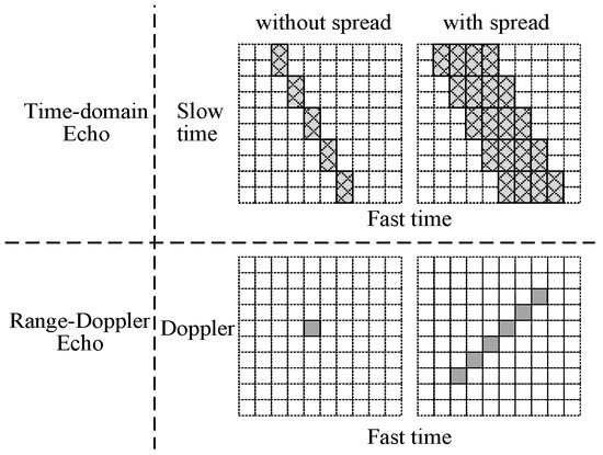
Figure 1. Time-domain echo and range-Doppler plane comparison of non-spread and spread Targets.

2.2. The Properties of Multi-Dimensional Spread Target

As illustrated in Figure 1, the range spread and the motion-parameters spread are the two main properties of the multi-dimensional spread target.

2.2.1. Analyses of the Property of Range Spread Target

Assuming that a spread target consists of evenly $2I$ spaced SCs and their spacing is $\mathrm{\Delta }D$, thus, the slant range $r_n$ between the n-the SC and the radar is given by

$$r_n=\sqrt{R^2+{\left(n\mathrm{\Delta }D\right)}^2+2Rn\mathrm{\Delta }Dcos\theta },$$

(3)

where R is the slant range from the radar to the target, $\theta$ is the elevation angle, and $n=-I,-I+1,\cdots ,I-1,I$ as shown in Figure 2. In the case of $R\ge D$, after Taylor expansion, (3) can be approximated as

$$r\left(t\right)\approx R+n\mathrm{\Delta }Dcos\theta .$$

(4)

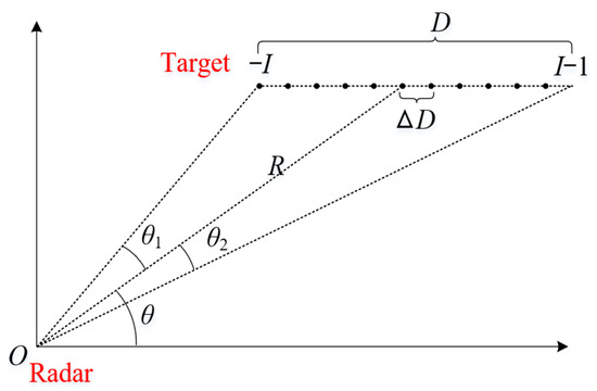
Figure 2. Schematic diagram of a range-spread target.

Thus, the projection length of the target in the direction of the radar line of sight is $Dcos\theta$. If the projection length is greater than one range resolution unit, i.e., $Dcos\theta >{\rho }_r$ is satisfied, then the target echo is actually spread in multiple range resolution units, i.e., spread in the range dimension, and the length of the target that falls in the same range resolution unit is given by

$$D_0=\frac{{\rho }_r}{cos\theta }.$$

(5)

2.2.2. Analyses of the Property of Multiple Motion Parameters

First, we will consider the case that the target does not rotate, and a schematic diagram has been provided to illustrate the geometry model and define each parameter, as shown in Figure 3.

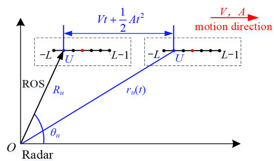
Figure 3. Schematic diagram under the case that the target does not rotate.

As shown in Figure 3, we select one SC of $2L$ SCs for simplicity, which is denoted as U with the distance $R_u$ from U to the radar and the angle ${\theta }_u$ between the motion direction and the radar line of sight (ROS). Moreover, $r_u\left(t\right)$ denotes the slant distance of U that changes with time, V denotes the velocity, and A denotes the acceleration. It should be noted that the derivation for the slant distance that changes with time of other SCs is the same. Thus, $r_u\left(t\right)$ can be written as

$$r\left(t\right)=\sqrt{R_u^2+{\left(Vt+\frac{1}{2}A{t}^2\right)}^2+2R_{u}cos{\theta }_u\left(Vt+\frac{1}{2}A{t}^2\right)}$$

(6)

where u is the distance from the target center to the SC, $R_u$ is the distance from the target center to the radar, V is the velocity, A is the acceleration, and ${\theta }_u$ is angle between the motion direction and the radar line of sight. Thus, the slant range at $t=0$ is $r\left(0\right)=R_u$, then after deriving $r\left(0\right)$ with respect to slant range R twice, we can get the velocity and acceleration of the target at $t=0$ as

$$\begin{array}{cc}\hfill r^{\prime }\left(0\right)& =Vcos{\theta }_u\hfill \\ \hfill r^{″}\left(0\right)& =Acos{\theta }_u+\frac{V^2{sin}^2{\theta }_u}{R_u}.\hfill \end{array}$$

(7)

Since the target consists of multiple SCs, the slant range $R_u$ and ${\theta }_u$ of each SC are different, thus, the velocity and acceleration of each SC are also different. Then, the speed difference between the two ends of the target is related to the change of the observation angle. As shown in Figure 2, if the radar line-of-sight angles between the left and right ends of the target and the target center are ${\theta }_1$ and ${\theta }_2$, respectively, then the speed difference between the two ends of the target is given by

$$\begin{array}{cc}\hfill \mathrm{\Delta }V& =V\left(cos\left(\theta -{\theta }_2\right)-cos\left(\theta +{\theta }_1\right)\right)\hfill \\ \hfill & \approx V\left({\theta }_2+{\theta }_1\right)sin\theta \approx \frac{VD{sin}^2\theta }{R}\hfill \end{array}$$

(8)

As for acceleration, it contains two terms, but the latter term is usually so small that the difference caused is negligible, thus, the difference in acceleration can be approximated as

$$\begin{array}{c}\hfill \mathrm{\Delta }A\approx A\left(cos\left(\theta -{\theta }_2\right)-cos\left(\theta +{\theta }_1\right)\right)\\ \hfill \approx A\left({\theta }_2+{\theta }_1\right)sin\theta \approx \frac{AD{sin}^2\theta }{R}\end{array}$$

(9)

It can be seen that the velocity difference $\mathrm{\Delta }V$ and the acceleration difference $\mathrm{\Delta }A$ at both ends of the target have a larger value when the slant range from the target to the radar is very close. Generally, $D/R$ is a very small amount, which means that the velocity difference $\mathrm{\Delta }V$ does not exceed one velocity resolution unit, and the acceleration difference $\mathrm{\Delta }A$ does not exceed one acceleration resolution unit, i.e., it can be regarded as the velocities and accelerations of the different SCs are the same, when the target does not rotate.

If the target rotates with an angular velocity of $\omega$, a schematic diagram has been given to shown the geometry model well as give the definition of each parameter, as shown in Figure 4.

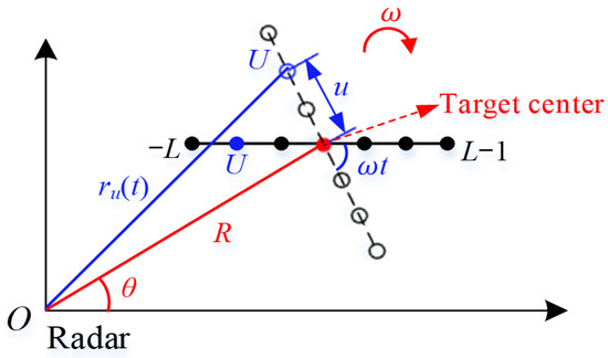
Figure 4. Schematic diagram under the case that the target rotates.

As shown in Figure 4, u denotes the distance from SC U to the center of target, $r_u\left(t\right)$ denotes the slant distance of U that changes with time, R denotes the distance from target center to radar, and $\theta$ denotes the angle between the target and ROS. Thus, $r_u\left(t\right)$ can be written as

$$r_u\left(t\right)=\sqrt{R^2+u^2+2Rucos\left(\omega t+\theta \right)}$$

(10)

After first and second-derivative operations, the velocity and acceleration of the SC can be obtained as

$$\begin{array}{cc}{r}_u\left(t\right)\hfill & =\sqrt{R^2+u^2+2Rucos\left(\omega t+\theta \right)}\hfill \\ r_u^{\prime }\left(0\right)\hfill & =\frac{-Ru\omega sin\theta }{r\left(0\right)}\approx -u\omega sin\theta \hfill \\ r_u^{″}\left(0\right)\hfill & =-\frac{Ru{\omega }^{2}cos\theta }{r\left(0\right)}-\frac{R^2{u}^2{\omega }^2{sin}^2\theta }{r^3\left(0\right)}\approx -u{\omega }^{2}cos\theta \hfill \end{array}$$

(11)

Then, the difference in velocity and acceleration between the two ends of the target is approximated as

$$\mathrm{\Delta }V\approx \omega Dsin\theta , \mathrm{\Delta }A\approx {\omega }^{2}Dcos\theta$$

(12)

In the case that the target speed is not fast, the acceleration difference $\mathrm{\Delta }A$ in (12) is usually negligible, and the speed difference $\mathrm{\Delta }V$, which represents the speed spread, should be analyzed according to the specific situation. In addition, according to radar imaging theory, Doppler in azimuth is proportional to instantaneous velocity, so the velocity spread in (12) can also be regarded as forming resolution capability in azimuth.

In general, the difference between range spread and motion spread is demonstrated in Figure 5, where the phenomenon of motion parameter spread is exemplified by velocity spread.

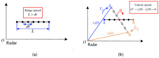
Figure 5. The difference between the phenomenon of range spread and motion spread. (a) The phenomenon of range spread; (b) The phenomenon of motion spread.

As shown in Figure 5a, D denotes the length of target and $dr$ denotes the range resolution. It should be noted that range spread will occur when D is larger than $dr$. Moreover, as shown in Figure 5b, $r_A\left(t\right)$ denotes the slant distance of A that changes with time, $r_B\left(t\right)$ denotes the slant distance of B that changes with time, $\omega$ denotes the rotation speed of the target, $\mathrm{\Delta }V$ denotes the difference of velocity, and $dv$ denotes the velocity resolution. It should be noted that velocity spread will occur when $\mathrm{\Delta }V$ is larger than $dv$.

2.3. The Length of Coherent Times

Assuming that the echoes of all SCs of the target are located in the same resolution unit. As shown in Figure 2, ignoring the influence of the envelope and constant phase, the target echo containing $2I$ SCs can be expressed as

$$y\left(\theta \right)=\sum _{n=-I}^{I-1}exp\left(-j\frac{4\pi f_c}{c}n\mathrm{\Delta }Dcos\theta \right)$$

(13)

Let $z=cos\theta$ and $u=\frac{2f_c\mathrm{\Delta }D}{c}$, $y\left(\theta \right)$ can be rewritten as

$$y\left(z\right)=\sum _{n=-I}^{I-1}exp\left(-j2\pi unz\right)$$

(14)

which means that the target echo is a periodic signal with a period of $1/u$. At this point, the autocorrelation function of the target echo can be obtained as

$$\begin{array}{c}\hfill R\left(\mathrm{\Delta }z\right)={\int }_{-\frac{1}{2u}}^{\frac{1}{2u}}y\left(z\right)y^{*}(z-\mathrm{\Delta }z)dz=exp(-j\pi u\mathrm{\Delta }z)\frac{2I}{u}\frac{sin\left(\pi u2I\mathrm{\Delta }z\right)}{sin\left(\pi u\mathrm{\Delta }z\right)}.\end{array}$$

(15)

The first zero-crossing point of the autocorrelation function is selected as the de-correlation length, then the de-correlation length can be written as

$$\mathrm{\Delta }z=\frac{1}{2uI}=\frac{c}{2f_{c}D}=\frac{\lambda }{2D}.$$

(16)

Assuming that the target angle changes very little, according to the relationship between z and $\theta$, after Taylor expansion, $\mathrm{\Delta }z$ can be approximated as

$$\mathrm{\Delta }z=cos\theta -cos\left(\theta -\mathrm{\Delta }\theta \right)\approx -\mathrm{\Delta }\theta sin\theta .$$

(17)

Therefore, the de-correlation angle can be approximated as

$$\mathrm{\Delta }\theta \approx \frac{\lambda }{2Dsin\theta }.$$

(18)

If the target is at a velocity V and moves at an angle $\theta$ with the radar line of sight, the decoherence time is approximated as

$$\mathrm{\Delta }T\approx \frac{\lambda R}{2VD{sin}^2\theta }.$$

(19)

Similarly, if the target rotates with angular velocity $\omega$, the decoherence time is approximated as

$$\mathrm{\Delta }T\approx \frac{\lambda }{2\omega Dsin\theta }.$$

(20)

For the spread target, the length of the target falling in the same range resolution unit is shown in (5), after substituting into (19) and (20), the decorrelation time in the two cases can be obtained as

$$\begin{array}{cc}\hfill \mathrm{\Delta }T& \approx \frac{\lambda R}{2V{\rho }_{r}sin\theta tan\theta },\hfill \\ \hfill \mathrm{\Delta }T& \approx \frac{\lambda }{2\omega {\rho }_{r}tan\theta }.\hfill \end{array}$$

(21)

where ${\rho }_r$ denotes the range resolution unit. It can be seen from (21) that, compared with the case of low-resolution and non-spread, although high-resolution causes the range spread phenomenon, since the effective length of the target falling into the same range resolution unit is reduced, the echo decoherence time will be correspondingly elongated, i.e., the echo coherence is stronger.

Based on the above analyses of the multi-dimensional spread target, we will propose several detection methods to detect the multi-dimensional spread target in following sections.

3. The Proposed Energy-Integrated GRFT Method

This section is dedicated to resolving the issue when the target exhibits only range spread and ARDU, and no prior information regarding the distribution of intensity and position of any SC is available, indicating that any intensity and position may occur with equal probability.

3.1. Echo Model

When the angle between the target motion direction and the radar line of sight is not large and the target does not rotate, the L SCs have the same motion parameters except the range $x_{1:K}={[x_1,x_2,...,x_K]}^T$, in which case only the range dimension spreads, known as the range spread target. For convenience, a vector is defined as follows, whose first element is 0.

$${\tilde{x}}_{1:K}={[0,x_1,x_2,...,x_K]}^T,$$

(22)

then the range from the l-th SC to the radar can be expressed as

$$r_{l,m}=r_l+\sum _{k=1}^K\frac{1}{k!}{x}_k{t}_m^k=r_l+r\left({\tilde{x}}_{1:K},t_m\right),$$

(23)

where $k=1,...,K$, $t_m$ is the slow time and K is the movement order of the range spread target. Moreover, $r_l$ is the initial range of the l-th SC, and $r\left({\tilde{x}}_{1:K},t_m\right)$ represents the range migration of the range spread target.

As shown in (23), the range spread is reflected in the difference of $r_l$, and the ARDU phenomenon is reflected in the change of $r\left({\tilde{x}}_{1:K},t_m\right)$ with $t_m$ superior.Then, the fast time-frequency domain form of the echo can be expressed as

$$\begin{array}{c}{S}_{m,q}=exp\left(-j{\omega }_{q}r\left({\tilde{x}}_{1:K},t_m\right)\right)Y_q{\displaystyle \sum _{l=0}^{L-1}}{a}_{l}exp\left(-j{\omega }_{q}r\right)=P_{m,q}\left(x_{1:K}\right)G_q,\end{array}$$

(24)

where $G_q$ is the spectrum of the one-dimensional (1-D) range profile of the range spread target (that is, the signal formed by the superposition of all SC echoes of the range spread target), including the information of the transmitted signal and target scattering characteristics. Moreover, $P_{m,q}\left({\tilde{x}}_{1:K}\right)$ is the phase caused by target motion in the fast time-frequency domain.

3.2. The Principle of Energy-Integrated GRFT

GRFT [51] can be achieved through joint envelope and phase compensation for every motion parameter $x_p$ in the multidimensional parameter space, whose algorithm flowchart is shown in Figure 6.

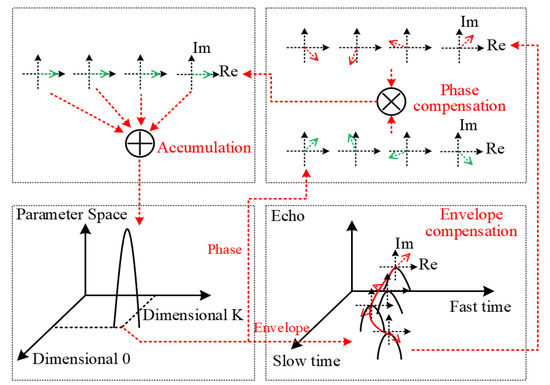
Figure 6. The algorithm flowchart of GRFT.

Specifically, the sampling grid is set as the search grid for range $x_{p,0}$, resulting in a special form of GRFT, i.e.,

$${\tilde{f}}_{GRFT}(n,x_{p,1:K})=\sum _{m=0}^{M-1}s\left(m,n+\frac{2f_s}{c}r({\tilde{x}}_{p,1:K},t_m)\right)exp\left(j\frac{4\pi f_c}{c}r({\tilde{x}}_{p,1:K},t_m)\right),$$

(25)

where $x_{p,1:K}$ is the vector composed of other motion parameters except range $x_{p,0}$, ${\tilde{x}}_{p,1:K}$ represents the vector with $x_{p,0}$ as 0, namely

$$\begin{array}{c}{x}_{p,1:K}={\left[x_{p,1},x_{p,2},...,x_{p,K}\right]}^T,\hfill \\ {\tilde{x}}_{p,1:K}=\left[0,x_{p,1},x_{p,2},...,x_{p,K}\right].\hfill \end{array}$$

(26)

Note that the constant phase factor corresponding to range $x_{p,0}$ can be ignored.

GRFT in the form of fast time-frequency domain can be obtained by DFT operation on ${\tilde{f}}_{GRFT}(n,x_{p,1:K})$ along n:

$${\tilde{F}}_{GRFT}(q,x_{p,1:K})=\sum _{m=0}^{M-1}{S}_{m,q}exp\left(j{\omega }_{q}r({\tilde{x}}_{1:K},t_m)\right).$$

(27)

In the following, we will derive the specific form of EI-GRFT based on the GLRT. According to the signal model, the binary hypothesis test of range spread target detection can be expressed as

$$\left\{\begin{array}{c}{H}_0:S_{m,q}=W_{m,q}\hfill \\ H_1:S_{m,q}=P_{m,q}\left(x_{1:K}\right)G_q+W_{m,q}\hfill \end{array}\right.,0\le m<M,0\le q<N,$$

(28)

where $W_{m,q}$ is the noise in the fast time-frequency domain.

Assume that $H_0$ is a simple hypothesis without unknown parameters; while $H_1$ is a compound hypothesis, whose unknown parameters are the motion parameter $x_{1:K}$ of the range spread target, the complex amplitude $a_0,a_1...,a_{L-1}$ of the SC and the spatial position $r_0,r_1...r_{L-1}$. It should be noted that the latter two are included in the spectrum $G={[G_0,G_1,...,G_{N-1}]}^T$ of the 1-D range image of the range spread target. In the absence of any prior information of the amplitude and position of the target SC, it can be considered that the echo of each range unit in the 1-D range image of the target is equally important. Therefore, the spectral estimation of the 1-D range image of the target can be used to replace the estimation of the amplitude and position of the SC, that is, $x_{1:K}$ and G are selected as unknown parameters.

Based on the Neiman Pearson criterion, the likelihood ratio test of (28) can be written as

$$\frac{p(S;G,x_{1:K},H_1)}{p(S;H_0)}\underset{H_0}{\overset{H_1}{\lessgtr }}\gamma ,$$

(29)

where S is the $N\times M$ size matrix composed of fast time-frequency domain echoes, whose q row and m column elements are $S_{m,q}$. $\gamma$ is the gate for judgment. Moreover, $p(S;H_0)$ and $p(S;G,x_{1:K},H_1)$ are the Probability Density Function (PDF) under the assumption of $H_0$ and $H_1$, respectively, which can be expressed as

$$p\left(S;G,x_{1:K},H_i\right)=\frac{1}{{\pi }^{MN}{\left({\sigma }^2\right)}^{MN}}exp\left(-\frac{1}{{\sigma }^2}{T}_i\right),i=0,1,$$

(30)

where

$$\begin{array}{cc}{T}_0={\displaystyle \sum _{m=0}^{M-1}}{S}_m^H{S}_m,& T_1={\displaystyle \sum _{m=0}^{M-1}}{\left(S_m-P_m\left(x_{1:K}\right)G\right)}^H\left(S_m-P_m\left(x_{1:K}\right)G\right)\end{array},$$

(31)

the m th column of S is denoted as $S_m$ with the size of $N\times 1$. Besides, the phase caused by the motion of target in the fast time-frequency domain echo is denoted as the diagonal matrix $P_m\left(x_{1:K}\right)$ with the size of $N\times N$. Additionally, $S_m$ and $P_m\left(x_{1:K}\right)$ are shown as

$$\begin{array}{c}{S}_m={[s_{m,0},s_{m,1},...,s_{m,N-1}]}^T\\ P_m\left(x_{1:K}\right)=diag\left\{P_{m,0}\left(x_{1:K}\right),P_{m,1}\left(x_{1:K}\right),...,P_{m,N-1}\left(x_{1:K}\right)\right\}.\end{array}$$

(32)

Then, the likelihood ratio test in (29) can be derived as

$$T_0-T_1\underset{H_0}{\overset{H_1}{\lessgtr }}\frac{1}{{\sigma }^2}ln\gamma .$$

(33)

Since G and $x_{1:K}$ is unknown, we need to find the MLE of the unknown parameter G and $x_{1:K}$, which is equivalent to finding the G and $x_{1:K}$ that maximize $p(S;G,x_{1:K},H_1)$, i.e. to minimize $T_1$. Thus, G with minimum $T_1$ is satisfied

$$\frac{\partial T_1}{\partial G^{*}}=MG-\sum _{m=0}^{M-1}{P}_m^H\left(x_{1:K}\right)S_m=0_{N\times 1},$$

(34)

where ${(·)}^{*}$ is a conjugate operation, and $0_{N\times 1}$ is the zero vector with the size of $N\times 1$. Based on (35), the MLE of G can be derived as

$$\widehat{G}=\frac{1}{M}\sum _{m=0}^{M-1}{P}_m^H\left(x_{1:K}\right)S_m=\frac{1}{M}\sum _{m=0}^{M-1}{S}_{m,q}exp\left(j{\omega }_{q}r({\tilde{x}}_{1:K},t_m)\right).$$

(35)

By comparing (27) and (35), we can find that ${\displaystyle \sum _{q=0}^{N-1}}{\tilde{F}}_{GRFT}(q,x_{p,1:K})$ is exactly M times the element ${\widehat{G}}_q$ of $\widehat{G}$. Further, $x_{1:K}$ that minimizes the $T_1$ can be obtained by traversal search. Then, GLRT can be simplified by substituting G into (33) as

$$\underset{x_{1:K}}{max}{\widehat{G}}^H\widehat{G}\underset{H_0}{\overset{H_1}{\lessgtr }}\frac{1}{M}{\sigma }^{2}ln\gamma .$$

(36)

Therefore, ${\widehat{G}}^H\widehat{G}$ in GLRT can be expressed as the energy of GRFT in the form of fast time-time domain according to Parseval’s theorem, namely

$${\widehat{G}}^H\widehat{G}=M^2\sum _{q=0}^{N-1}{\tilde{f}}_{GRFT}(n,x_{p,1:K}){\tilde{f}}_{GRFT}^{*}(n,x_{p,1:K}).$$

(37)

In practice, only a small part of all range units is occupied by the range spread target, so it is necessary to use sliding window operation to search all range units. This process is defined as EI-GRFT, which is expressed in a continuous form as

$$f_{EI-GRFT}\left(x_p\right)={\left|f_{GRFT}\left(x_p\right)\right|}^2{*}_{s}rec{t}_s\left(\frac{x_{p,0}}{x_{w,0}}\right),$$

(38)

where ${*}_s$ denotes convolution operation, $rec{t}_s(·)$ denotes rectangular window, and $x_{w,0}$ denotes the length of the detection window.

Therefore, (36) can be written in the form of EI-GRFT as follows

$$\underset{x}{max}{f}_{EI-GRFT}(n,x_{p,1:K})\underset{H_0}{\overset{H_1}{\lessgtr }}M{\sigma }^{2}ln\gamma .$$

(39)

Further, the goal of fast realization of EI-GRFT can be achieved combined with the fast method of GRFT.

According to the derivation process of EI-GRFT in Section 3, EI-GRFT is more suitable for the case that the echo energy of all units in the detection window is generally the same, which means that the SCs of the target is very dense. In practice, there may be cases where the distribution of SCs is sparse, thus, the target echo is mainly composed of echoes from a few SCs, in which case the detection performance of EI -GRFT will be declined. To solve this problem, we will propose the DT-HGRFT method in the next section.

4. The Proposed Double-Threshold Hybrid GRFT Method

This section presents the proposal of DT-HGRFT, which aims to further enhance the detection performance of multi-dimensional spread targets. Initially, HGRFT is utilized to enable the inter-pulse integration of single SC echoes having ARDU and decoherence phenomena. Then, the units within the multi-dimensional detection window are selectively re-integrated by setting the first threshold to filter out the units that might have SCs for further integration. Finally, the target is detected by determining whether the integration result surpasses the second threshold.

4.1. Brief Introduction for HGRFT

HGRFT is a method used to achieve hybrid integration of the echo signal, which is based on both GRFT and non-coherent integration. As shown in Figure 7, HGRFT divides the full aperture into multiple sub-apertures and implements a two-step integration operation, which consists of the coherent integration within each sub-aperture by GRFT and noncoherent integration among multiple sub-apertures.

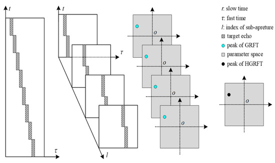
Figure 7. The algorithm flowchart of HGRFT.

Initially, GRFT is performed within the sub-apertures, namely:

$$f_{GRFT}(k,x_p)=\sum _{j=0}^{T_c}s\left(j,\frac{2f_s}{c}r(x_p,t_j+j{T}_c)\right)exp\left(j\frac{4\pi f_c}{c}r(x_p,t_j+j{T}_c)\right),$$

(40)

where k is the indexing number of the sub-aperture, $T_c$ is the length of each sub-aperture. Then, the GRFT integration results of each sub-aperture are non-coherently accumulated, which can be expressed as

$$f_{HGRFT}\left(x_p\right)=\sum _{k=1}^{{N^{\prime }}_c}{\left|f_{GRFT}(k,x_p)\right|}^2,$$

(41)

where ${N^{\prime }}_c$ is the number of sub-apertures.

4.2. DT-HGRFT within Sparse Distribution of Scattering Centers

In order to avoid integrating additional noise, it is necessary to screen the integrated units when SCs are sparsely distributed.

4.2.1. The Number of Scattering Centers Is Known

Assuming that the echo contains only one pulse, and the signal on the units that contain the target in the pulse is defined as

$$s={\left[s_0,s_1,...,s_{N-1}\right]}^T,$$

(42)

then the binary hypothesis test can be written as

$$\left\{\begin{array}{c}{H}_0:s=w\hfill \\ H_1:s=g+w\hfill \end{array}\right.,$$

(43)

where w is the complex Gaussian white noise with power of ${\sigma }^2$, and g is the target echo. When the number of SCs L contained in the target is less than the number of occupied units N, only L non-zero elements exist in g, and the other elements are 0.

Under the assumption of $H_1$, the PDF of the received signal can be written as

$$p(s;H_1)=\frac{1}{{\pi }^N{\left({\sigma }^2\right)}^N}exp\left(-\frac{1}{{\sigma }^2}\sum _{n=0}^{N-1}{\left|s_n-g_n\right|}^2\right).$$

(44)

In order to obtain the MLE of the value and position of these L elements, it is necessary to maximize $p_{s;H_1}$, which is equal to minmize the sum term in the exponential part of (44). It can be seen that when the L non-zero elements of g are equal to the elements of s at the same position, the sum term is the sum of the squares of the modules of the $N-L$ elements in s, and the number of the sum terms is the minimum. Moreover, if the sum element is minimized at the same time, the total sum term can be minimized. At this time, the MLE of the non-zero element of g and its position is the value and position of the L elements with the largest modulus in the echo s, and the sum term is the square sum of the modules of the $N-L$ elements with the smallest modulus in s.

Arranging the received signals in descending order of module, and the result is shown as

$$\begin{array}{cc}{s}^{\prime }={\left[{s^{\prime }}_0,{s^{\prime }}_1,···,{s^{\prime }}_{N-1}\right]}^T,& \left|{s^{\prime }}_0\right|\end{array}\ge \left|{s^{\prime }}_1\right|\ge ···\left|{s^{\prime }}_{N-1}\right|.$$

(45)

Then, $p(s;H_1)$ can be simplified by substituting the non-zero element of g and its MLE position into the PDF of the received signal, as

$$p(s;H_1)=\frac{1}{{\pi }^N{\left({\sigma }^2\right)}^N}exp\left(-\frac{1}{{\sigma }^2}\sum _{n=L}^{N-1}{\left|{s^{\prime }}_n\right|}^2\right).$$

(46)

Under the assumption of $H_0$, the PDF of the received signal can be written as

$$p(s;H_0)=\frac{1}{{\pi }^N{\left({\sigma }^2\right)}^N}exp\left(-\frac{1}{{\sigma }^2}\sum _{n=0}^{N-1}{\left|{s^{\prime }}_n\right|}^2\right).$$

(47)

Therefore, GLRT can be written as

$$\sum _{n=0}^{L-1}{\left|{s^{\prime }}_n\right|}^2\underset{H_0}{\overset{H_1}{\lessgtr }}{\sigma }^{2}ln\gamma .$$

(48)

It can be seen that the test statistic is the energy of L units with the largest received signal module.

4.2.2. The Number of Scattering Center Is Unknown

In practice, the number of SCs present in the received signal is often unknown and needs to be estimated. To achieve this, a low threshold is utilized to determine whether each unit has SCs, which is referred to as the first threshold. The estimated number of SCs L can then be determined as the number of units that pass the first threshold, which can be mathematically expressed as follows:

$$\widehat{L}=\sum _{n=0}^{N-1}B\left(n\right),$$

(49)

where $B\left(n\right)$ represents the judgment result of the first threshold $V_{T,1}$, namely

$$B\left(n\right)=\left\{\begin{array}{cc}0,& {\left|s_n\right|}^2<V_{T,1}\\ 1,& {\left|s_n\right|}^2\ge V_{T,1}\end{array}\right..$$

(50)

Then, the test statistic T can be reduced by substituting L into GLRT, as

$$T=\sum _{n=0}^{N-1}B\left(n\right){\left|s_n\right|}^2.$$

(51)

Corresponding to the first threshold, the threshold in GLRT to judge the test statistic T is called the second threshold. Consequently, the principle of double-threshold detection is shown in Figure 8.

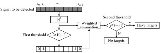
Figure 8. Schematic diagram of single double-threshold detection principle.

4.3. Hybrid Intergation under Echo Decorrelation

From the perspective of integrating over the slow-time dimension, it is evident that GLRT depends on the statistical properties of the echo signal, rather than being in the form of complete coherent integration in the presence of echo decoherence. However, in practice, the statistical properties of the echo signal must be estimated from the measured data, which results in a considerable operational burden on the GLRT detector.

To illustrate, let us consider the case where the echo follows a Gaussian distribution and is assumed to be in the same range unit for simplicity. In this scenario, the detection task is to detect colored Gaussian noise in Gaussian white noise, and its GLRT can be expressed as:

$$z^H{C}_s{\left(C_s+{\sigma }^{2}I\right)}^{-1}z\underset{H_0}{\overset{H_1}{\lessgtr }}{\gamma }^{\prime },$$

(52)

where z is the column vector signal, $C_s$ is the covariance matrix of the signal to be detected, and ${\gamma }^{\prime }$ is the threshold. The statistical characteristics of the signal to be detected are described by $C_s$, which usually needs to be estimated from the measured data. Therefore, the matrix inversion operation in GLRT also needs to be carried out dynamically, resulting in a huge amount of computation.

In order to solve the problem of echo decoherence concisely and efficiently, the method of mixed integration is adopted to accumulate in the slow time dimension. The mixed integration is only GLRT under the condition of fully coherent molecular pore size, and there is a little performance loss under the condition of slow change of actual correlation. However, its simple implementation can greatly reduce the amount of computation. Moreover, the integration of the slow time dimension takes the form of HGRFT combined with the ARDU problem.

4.4. Sliding Window Detection under Multi-Dimensional Spread Conditions

When the angle between the direction of target movement and the radar line of sight is large or when the target rotates, the change in the angle of radar observation cannot be ignored. In such cases, the target’s other motion parameters may not be the same except for the range. To accumulate the echoes of all SCs, multi-dimensional integration is required. Moreover, the target’s motion parameters may vary over a large range, but each occurrence only occupies a small part of the parameter space. Therefore, it is necessary to search all possible motion parameters, which involves multi-dimensional sliding window detection with a total number of detection window units of $N_w$ in the parameter space.

Based on the analysis of the target spread characteristics, it is found that only some of the motion parameters may exhibit spread in practical scenarios. In such cases, sliding window detection can be carried out only in the dimension of the spread parameters, while the sequential processing can be conducted in the dimension of the non-spread parameters. For instance, if the movement or rotation of the target causes range and velocity dimensions to spread, but the acceleration dimension typically does not spread, then only the sliding window integration of the range and velocity dimensions is required in the integration results on the multi-dimensional parameter space. This is illustrated in Figure 9. The echoes of SCs with different ranges and velocities have certain orthogonality, which reduces the mutual influence of different SCs and facilitates the integration of different elements. Moreover, prior information about the target scattering characteristics can be useful in selecting the multi-dimensional detection window.

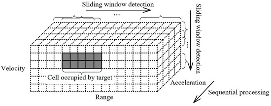
Figure 9. Two-dimensional sliding window detection in the three-dimensional parameter space of range-velocity-acceleration.

4.5. DT-HGRFT & Its Relationship with GRFT and EI-GRFT

Considering the two dimensions of SC and slow time, DT-HGRFT is defined as the form of multi-dimensional sliding window and double-threshold detection for the results of HGRFT, which can be realized by convolution operation, i.e.,

$$f_{DT-HGRFT}\left(x_p\right)=\left(f_{HGRFT}\left(x_p\right)B\left(x_p\right)\right){*}_{m}rec{t}_m\left(\frac{x_{p,0}}{x_{w,0}},\frac{x_{p,1}}{x_{w,1}},...,\frac{x_{p,K}}{x_{w,K}}\right).$$

(53)

where ${*}_m$ represents multi-dimensional convolution operation, $x_{w,k}$ represents the length of the k-th dimension of the detection window, $N_w$ represents the product of the size of the multiple dimensions of the detection window, and $B\left(x_p\right)$ is the judgment result of HGRFT output using the first threshold, namely

$$B\left(x_p\right)=\left\{\begin{array}{cc}0,& f_{HGRFT}\left(x_p\right)<V_{T,1}\\ 1,& f_{HGRFT}\left(x_p\right)\ge V_{T,1}\end{array}\right..$$

(54)

It should be noted that HGRFT is the sum of the modular squares of the GRFT results on multiple sub-apertures, and there is no modular square operation here. It can be seen that DT-HGRFT is a combination of HGRFT and double-threshold detection method. Specifically, HGRFT is conducted to accumulate the echo with ARDU and de-coherence phenomenon between pulses, and multi-dimensional sliding window double-threshold detection is further conducted to accumulate the SC echo distributed on multiple dimensions. Unlike single-pulse double-threshold detection, DT-HGRFT is a double-threshold detection after a long time of integration, which is applicable to the case of lower SNR by using the integration gain.

From the perspective of SC distribution, the units containing SCs can be screened out as much as possible through the first threshold in DT-HGRFT, which needs an appropriate size to obtain better screening results. In the special case that each unit in the detection window contains SCs, it is obvious that the first threshold should set to 0 to ensure that all units participate in the integration. Consequently, DT-HGRFT degenerates into EI-HGRFT

$$f_{EI-HGRFT}\left(x_p\right)=f_{HGRFT}\left(x_p\right){*}_{m}rec{t}_m\left(\frac{x_{p,0}}{x_{w,0}},\frac{x_{p,1}}{x_{w,1}},···,\frac{x_{p,K}}{x_{w,K}}\right).$$

(55)

From the perspective of echo coherence, DT-HGRFT uses a combination of GRFT coherent integration within sub-aperture and direct non-coherent integration between sub-apertures in the slow time dimension, so the selection for the length of sub-aperture directly affects the detection performance. Correspondingly, the length of sub-aperture needs to be lengthened to carry out coherent integration as long as possible. For the case that the echo is completely coherent within the integration time, it is obvious that the optimal performance can be achieved by setting the number of sub-apertures to 1. At this time, considering that GRFT is HGRFT with 1 sub-aperture, DT-HGRFT can also called DT-GRFT in the case of full coherence, namely

$$f_{DT-HGRFT}\left(x_p\right)=\left({\left|f_{GRFT}\left(x_p\right)\right|}^{2}B\left(x_p\right)\right){*}_{m}rec{t}_m\left(\frac{x_{p,0}}{x_{w,0}},\frac{x_{p,1}}{x_{w,1}},···,\frac{x_{p,K}}{x_{w,K}}\right).$$

(56)

It should be noted that $B\left(x_p\right)$ is the judgment result of GRFT output using the first threshold, namely

$$B\left(x_p\right)=\left\{\begin{array}{cc}0,& {\left|f_{GRFT}\left(x_p\right)\right|}^2<V_{T,1}\\ 1,& {\left|f_{GRFT}\left(x_p\right)\right|}^2\ge V_{T,1}\end{array}\right..$$

(57)

Moreover, when adopting full coherent integration and setting the first threshold to 0 at the same time, DT-HGRFT degenerates into multi-dimensional integration EI-GRFT, namely

$$f_{EI-HGRFT}\left(x_p\right)={\left|f_{GRFT}\left(x_p\right)\right|}^2{*}_{m}rec{t}_m\left(\frac{x_{p,0}}{x_{w,0}},\frac{x_{p,1}}{x_{w,1}},···,\frac{x_{p,K}}{x_{w,K}}\right).$$

(58)

It should be noted that the EI-GRFT in (58) is multi-dimensional integration

Generally, the conversion between DT-HGRFT, EI-HGRFT, DT-GRFT, EI-GRFT and traditional HGRFT and GRFT is shown in Figure 10.

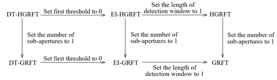
Figure 10. Simplification of DT-HGRFT in special cases.

4.6. Joint Detection of Multiple DT-HGRFT

In the double-threshold detection approach, the initial threshold assessment is aimed at estimating the number of sub-carriers (SCs). Although alternative techniques are available for SCs estimation, such as the maximum inter-class variance method [52], two-mean clustering [53], etc., they generally require further search or iteration. In contrast, the use of the initial threshold judgment represents a simple and efficient method. This is particularly relevant in scenarios of multi-dimensional sliding window analysis within the parameter space, where the SCs number at all locations can be promptly calculated through Fast Fourier Transform (FFT) application.

The first threshold in [41] is selected as a fixed value independent of the number of SCs. The first threshold in [42] is set according to the false alarm probability of the judgment, which is a simple and direct method. In fact, the optimal first threshold should be related to the number of SCs. Specifically, when the number of SCs is small, a higher first threshold should be selected to eliminate the units containing noise as much as possible, while when the number of SCs is large, a lower first threshold should be selected to minimize the units containing SCs.

In practical applications, only the largest units can be integrated when the number of SCs is exactly known. However, this will involve sorting operations, resulting in a large increase in the amount of computation. It should be noted that the first threshold judgment is a method with less computation, and the optimal first threshold simulated in advance can be applied when the number of SCs is known exactly. Besides, the optimal first threshold can also be roughly obtained by simulation when the number of SCs is known to be distributed in a small range.

However, the more complex case is that the number of SCs has a large distribution range or there is no information about the number of SCs. In this case, $N_{T1}$ DT-HGRFT with different first threshold can be used for joint detection. Specifically, a target is judged to be existed as long as DT-GRFT detects once, which can approach the detection performance with the optimal first threshold. In this case, the relationship between the total false alarm probability and each detection false alarm probability is

$$P_{fa,total}=1-{(1-P_{fa})}^{N_{T1}}\approx N_{T1}{P}_{fa}.$$

(59)

Then the false alarm probability of each detection should be approximately set to $1/N_{T1}$ of the total false alarm probability, which can be verified in simulation in in Section 5.

5. Theoretical Analyses of the EI-GRFT and DT-HGRFT

5.1. The Relationship between Threshold and False Alarm Probability of EI-GRFT

Assuming that the time domain noise is independent and follows a zero-mean complex Gaussian distribution with variance ${\sigma }^2$. Under the assumption of $H_0$, the noise after GRFT is the sum of M independent and identically distributed(IID) complex Gaussian random variables, which follows the complex Gaussian distribution with a mean value of 0 and variance of $M{\sigma }^2$. Therefore, the result of EI-GRFT is the sum of squares of $2N_w$ IID zero-mean Gaussian random variables, whose normalized result follows the chi-square distribution, i.e.,

$$\frac{2}{M{\sigma }^2}{f}_{EI-GRFT}(n,x_{p,1:K})\sim {\chi }^2\left(2N_w\right).$$

(60)

Further, the relationship between false alarm probability $P_{fa}$ and detection threshold $V_T$ can be derived as

$$\begin{array}{cc}{P}_{fa}=Q_{{\chi }^2}(\frac{2V_T}{M{\sigma }^2},2N_w),& V_T=\frac{M{\sigma }^2}{2}{Q}_{{\chi }^2}^{-1}(P_{fa},2N_w)=V_0{P}_n,\end{array}$$

(61)

where ${\chi }^2\left(2N_w\right)$ represents the chi-square distribution with a degree of freedom of $2N_w$, $Q_{{\chi }^2}(·,2N_w)$ represents the right tail probability of ${\chi }^2\left(2N_w\right)$, ${(·)}^{-1}$ represents the inverse function, and $P_n=N_{w}M{\sigma }^2$ is the integrated noise power. Moreover, $V_0$ is the threshold factor, which is shown as

$$V_0=\frac{1}{2N_w}{Q}_{{\chi }^2}^{-1}(P_{fa},2N_w).$$

(62)

5.2. The Detection Probability Analyses of EI-GRFT

Under the assumption of $H_1$, the result of EI-GRFT is the sum of squares of $2N_w$ IID non-zero mean Gaussian random variables, whose normalized result follows the decentralized chi-square distribution, namely

$$\frac{2}{M{\sigma }^2}{f}_{EI-GRFT}(n,x_{p,1:K})\sim {\chi }^{\prime 2}(2N_w,{\lambda }_0).$$

(63)

Therefore, the detection probability can be derived as

$$\begin{array}{c}{P}_d=Q_{{{\chi }^{\prime }}^2}\left(\frac{2V_T}{M{\sigma }^2},2N_w,{\lambda }_0\right)=Q_{{{\chi }^{\prime }}^2}\left(Q_{{\chi }^2}^{-1}(P_{fa},2N_w),2N_w,2M{r}_{SNR}\right),\end{array}$$

(64)

where ${\chi }^{\prime 2}(2N_w,{\lambda }_0)$ represents a decentralized chi-square distribution with a degree of freedom of $2N_w$ and a non-central parameter of ${\lambda }_0$, whose right tail probability is $Q_{{{\chi }^{\prime }}^2}(·,2N_w,{\lambda }_0)$. Moreover, the non-central parameter ${\lambda }_0$ can be shown as

$${\lambda }_0=\frac{2}{M{\sigma }^2}{M}^{2}E=2M{r}_{SNR},$$

(65)

where E represents the energy of the echo of the range spread target in a single pulse. $r_{SNR}$ represents SNR, which can be defined as

$$r_{SNR}=\frac{E}{{\sigma }^2}.$$

(66)

5.3. Analyses of the Second Thresholds of DT-GRFT and DT-HGRFT

The total false alarm probability of DT-HGRFT is the weighted sum of the false alarm probability of each case according to the probability of occurrence of this case. Moreover, considering that $\widehat{L}=0$ is always judged as no target, that is, no false alarm occurs, the total false alarm probability can be written as

$$P_{fa}=\sum _{\widehat{L}=1}^{L}P\left(\widehat{L}\right)P_{fa}\left(\widehat{L}\right),$$

(67)

where $P\left(\widehat{L}\right)$ is the probability of the occurrence of the case where the number of SCs is estimated to be L, and $P_{fa}\left(\widehat{L}\right)$ is the false alarm probability in this case. Under different $\widehat{L}$ conditions, $P_{fa}\left(\widehat{L}\right)$ can be maken to be equal by setting different second thresholds, then

$$P_{fa}\left(\widehat{L}\right)=\frac{P_{fa}}{1-P\left(0\right)}.$$

(68)

Additionally, $P\left(0\right)$ is very small when the first threshold is small, and it can be considered that $P_{fa}\left(\widehat{L}\right)\approx P_{fa}$.

5.3.1. The Second Threshold Setting of DT-HGRFT

It is important to note that the false alarm probability of DT-HGRFT is dependent on the first threshold and the estimation of the number of SCs, which poses difficulties in theoretical and simulation analyses. In theory, the HGRFT results lose their chi-square distribution form after the first threshold judgment. In simulations, the probability of occurrence is too low when both the first threshold and the estimated number of SCs are large, making it challenging to simulate enough samples. Therefore, this paper classifies cases where the first threshold differs but the number of SCs is estimated to be the same. The same second threshold is applied in this paper to simplify the theoretical and simulation analyses, even though it may not be optimal.

It should be noted that the second threshold setting of DT-HGRFT involves the sequencing of random variables. Therefore, some basic knowledge of random variable sequencing are given first. After sorting the random variables of K IIDs from small to large, the PDF and Cumulative Distribution Function (CDF) of the k-th ordered sample can be written as follows [54] respectively

$$\begin{array}{c}{f}_k\left(x\right)=k{C}_K^k{(1-F(x\left)\right)}^{K-k}{\left(F\right(x\left)\right)}^{k-1}f\left(x\right),\\ F_k\left(x\right)={\displaystyle \sum _{i=k}^K}{C}_K^k{\left(1-F\left(x\right)\right)}^{K-i}{\left(F\left(x\right)\right)}^i,\end{array}$$

(69)

where $f\left(x\right)$ and $F\left(x\right)$ are the PDF and CDF of the K random variables respectively. Besides, $C_K^k$ represents the combined number of k elements taken from the K different elements.

The second threshold of DT-HGRFT is related to the number of sub-apertures ${N^{\prime }}_c$, the estimated number of SCs L and the noise power $P_n$, which can be written as

$$V_{T,2}=V_{0,2}\widehat{L}{N}_c^{\prime }{P}_{n,0}=V_{0,2}{\widehat{L}}_c{P}_n,$$

(70)

where $P_{n,0}$ represents the noise power before the incoherent integration between sub-apertures. $P_n$ represents the noise power after HGRFT, which follows the chi-square distribution with a degree of freedom of $2{N^{\prime }}_c$ after normalization. Besides, $V_{0,2}$ is the second threshold factor used to adjust the false alarm probability.

When the number of SCs is estimated to be $\widehat{L}=1$, the test statistic of DT-HGRFT is the largest ordered sample. Therefore, the relationship between false alarm probability $P_{fa}$ and threshold factor $V_{0,2}$ as well as detection window length $N_w$ can be obtained by substituting the CDF of chi-square distribution into (69), as

$$P_{fa}=1-{\left(1-Q_{{\chi }^2}(2{N^{\prime }}_c{V}_{0,2},2N^{\prime })\right)}^{N_w}.$$

(71)

When the estimated number of SCs L is equal to the detection window length $N_w$, DT-HGRFT degenerates into EI-HGRFT. Moreover, the relationship between false alarm probability $P_{fa}$ and threshold factor $V_{0,2}$ is similar to that in (61), which can be written as

$$\begin{array}{cc}{P}_{fa}=Q_{{\chi }^2}(2N_w{N^{\prime }}_c{V}_{0,2},2N_w{N^{\prime }}_c),& V_{0,2}=\frac{1}{2N_w{N}^{\prime }}\end{array}{Q_{{\chi }^2}}^{-1}(P_{fa},2N_w{N}_c^{\prime }).$$

(72)

Additionally, the second threshold factor can be obtained through simulation experiments in other cases.

5.3.2. The Second Threshold Setting of DT-GRFT

When the number of sub-aperture is 1, the DT-HGRFT will be reduced to DT-GRFT, thus, we will analyze the second threshold setting of DT-GRFT in this section.

First, the effect of the first threshold screening on random variable PDF in general is discussed. For the random variable x with PDF and CDF of $f\left(x\right)$ and $F\left(x\right)$ respectively, the first threshold $V_{T,1}$ is conducted to filter (the case less than $V_{T,1}$ is discarded instead of zero) and get the random variable y. Then the PDF of random variable $\mathrm{\Delta }y=y-V_{T,1}$ is

$$\begin{array}{cc}{f}_{\mathrm{\Delta }y}\left(\mathrm{\Delta }y\right)=\frac{f(\mathrm{\Delta }y+V_{T,1})}{1-F\left(V_{T,1}\right)},& \mathrm{\Delta }y\ge 0.\end{array}$$

(73)

In particular, the PDF and CDF of random variables can be found to remain unchanged during this process in the case of exponential distribution.

Since GRFT is a completely coherent integration, the result after taking the square of its modulus follows the exponential distribution. Further, the random variables obtained follow the chi-square distribution after subtracting the first threshold, summing and normalizing the units selected from the first threshold. Thus, the relationship between the second threshold $V_{T,2}$ of DT-GRFT and the false alarm probability $P_{fa}\left(\widehat{L}\right)$ is

$$\begin{array}{c}{P}_{fa}\left(\widehat{L}\right)=Q_{{\chi }^2}\left(\frac{2(V_{T,2}-\widehat{L}{V}_{T,1})}{P_n},2\widehat{L}\right),\hfill \\ V_{T,2}=\widehat{L}{V}_{T,1}+\frac{1}{2}{Q_{{\chi }^2}}^{-1}(P_{fa}\left(\widehat{L}\right),2\widehat{L})P_n.\hfill \end{array}$$

(74)

Moreover, the form written as threshold factor is

$$V_{0,2}=V_{0,1}+\frac{1}{2\widehat{L}}{Q_{{\chi }^2}}^{-1}(P_{fa}\left(\widehat{L}\right),2\widehat{L}),$$

(75)

where $V_{0,1}$ and $V_{0,2}$ are the first and second threshold factors respectively, which can be written as

$$\begin{array}{cc}{V}_{T,1}=V_{0,1}{P}_n,& V_{T,2}=V_{0,2}\widehat{L}{P}_n,\end{array}$$

(76)

where $P_n$ represents the noise power after GRFT.

It can be seen that the second threshold of DT-GRFT is not only related to the first threshold, but also related to the number of SCs estimated by the first threshold judgment. Additionally, compared with EI-GRFT, the second threshold of DT-GRFT has added an item representing the first threshold in addition to the change in the degree of freedom of the chi-square distribution.

6. Numerical Simulations and Experimental Results

In this section, we will perform simulations to analyze the impact of the second threshold on false alarm probability, the effect of the first threshold on detection performance, and evaluate the detection performance of our proposed method. Additionally, we will also conduct real data experiments to verify the effectiveness of our approach.

6.1. Simulation of the Influence of the First and Second Thresholds

The Influence of the Second Threshold on the False Alarm Probability

First, we will consider how to set the second threshold when only Gaussian noise is present. Specifically, we will analyze the relationship between the second threshold and false alarm probability through Monte Carlo simulation experiments, where the number of Monte Carlo experiments is set to ${10}^9$.

Since the second threshold of DT-HGRFT needs to be obtained through simualtion experiments, let the first threshold factor set to 1, we can simulate the relationship between $P_{fa}$ and the second threshold factor in the two special cases where the estimated number of SCs $\widehat{L}$ is 1 and $N_w$. The comparison of the theoretical and simulation results of the $P_{fa}$ is shown in Figure 11a, which shows that the simulation results under different conditions are consistent with the theoretical results.

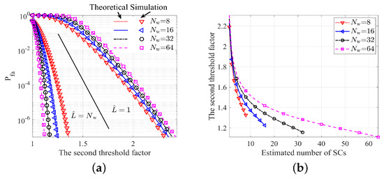
Figure 11. The relationship between the $P_{fa}$ of DT-HGRFT and the second threshold factor. (a) The $P_{fa}$ in two special cases ($\widehat{L}=1,N_w$). (b) The relationship between threshold factor and estimated number of SCs.

In practice, the second threshold is normally determined by the $P_{fa}$, and the second threshold factor curve is obtained using interpolation when the $P_{fa}$ is set to ${10}^{-6}$, as illustrated in Figure 11b. It should be noted that the total energy integrated by DT-HGRFT increases with the increase of $\widehat{L}$. However, since the units with samller amplitudes are integrated later, the power of each unit after averaging to $\widehat{L}$ units is decreasing. Thus, the second threshold factor steadily declines with the increase of $\widehat{L}$. In addition, when $\widehat{L}$ is fixed, the larger $N_w$ is, the greater the total energy of the largest $\widehat{L}$ units is. Hence, the second threshold factor gradually increases with the increase of $N_w$.

6.2. Simulation of the Influence of the First Threshold on Detection Performance

In order to illustrate the influence of the first threshold on DT-HGRFT, Monte Carlo simulation experiments are carried out. The parameters of the simulation experiments, The number of experiments was 1000 times, $P_{fa}$ is set to ${10}^{-6}$, the integrated pulse number is 1280, the detection window size is 64, the number of target SCs varies from 1 to 64, and the energy of different SCs of the same target is the same and the total energy is 1.

Based on above parameters, we conduct the simulation experiments of the detection performance (including detection probability ($P_d$ ), the required SNR and the first threshold factor) of DT-HGRFT, and the corresponding results are listed in Figure 12a–c, when the number of sub-apertures is 32. Figure 12a depicts the $P_d$ curve of the DT-HGRFT when the SNR is −9 dB following pulse compression; Figure 12b shows the required SNR curve with the first threshold factor when $P_d=0.9$; Figure 12c shows values of the first threshold factor with the number of SCs L (the blue lines). It should be noted that the extracted first threshold factors for each number of SCs are not represented by a single value, but rather a range, as indicated by the blue dots in Figure 12c. Specifically, Figure 12c displays a curve of the fitted first threshold factors versus the number of SCs, and the fitted first threshold factors have been extracted based on the data presented in Figure 12b. However, Figure 12c displays the simulation result, which is not smooth and may lead to inaccurate results when identifying the first threshold factor corresponding to the minimum value in Figure 12b. To address this issue, we have extracted the first threshold factor under the condition that the SNR requirement is in the region of the lowest 0.2 dB. Consequently, when the number of SCs is large, that is, above 32, a broad range of extracted first threshold factors can be obtained. Moreover, the first threshold factor is extracted under the condition that the SNR requirement is in the region of the lowest 0.2 dB, then, the fitting results with $2.02L^{-0.2106}$ is shown as well (the red line in Figure 12c).

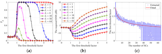
Figure 12. The relationship between the detection performances of DT-GRFT and DT-HGRFT and the first threshold, and the left column is the results of DT-GRFT, and the right column is the results of DT-HGRFT. (a) is $P_d$ curves of DT-HGRFT, when the SNR is −9 dB. (b) is the required SNR curve of DT-HGRFT, when $P_d=0.9$. (c) is the fitted first threshold factor curve of DT-HGRFT.

Specifically, we can draw the following comparison results: (1) When the first threshold factor is very small, almost all the units will exceed the threshold. (2) For the case where the number of SCs L is small, only the first threshold factor with an appropriate value can accurately extract the units containing the SCs. If the value is too small, too much noise will be introduced, and if the value is too large, the SCs are missing. (3) A smaller first threshold factor should be chosen when L is large in order to extract as many units containing SCs as possible. In particular, when $L\ge$ 32, the best detection probability can be achieved when the first threshold factor close to 0. Additionally, from overall view, the best initial threshold factor progressively drops when L increases.

In practice, the number of SCs is typically unknown. In this case, several first thresholds may be employed to perform multiple joint detections. The results of DT-HGRFT are shown in Figure 13, where the three first threshold factors are selected as 0.75, 1.25 and 1.5, and the first threshold factor of the single-time first threshold detection method varies from 0 to 5 at an interval of 0.025. From the results in Figure 13, we can see that the performance of the three-times joint detection method is colse to the detection performance when using the optimal first threshold factor.

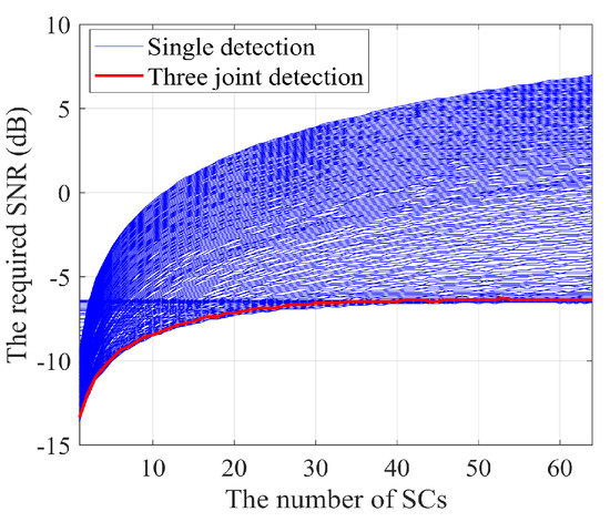
Figure 13. The performance comparison results of single detection and three joint detections of DT-HGRFT.

6.3. Simulation of Detection Performance

To compare the detection performance of different methods, i.e., the GRFT, EI-GRFT, HGRFT, EI-HGRFT, DT-GRFT, DT-HGRFT and EI-KT (energy-integrated keystone transform), we conduct Monte Carlo simulation experiments in the sub-section. The simulation parameters are shown in Table 1, and the target parameters and processing parameters are shown in Table 2. Note that when the number of SCs changes, the total energy of different SCs keeps the same. In the simulation experiments, the first threshold factors of DT-HGRFT is set according to the above fitting results in Figure 12, for the cases of different numbers of SCs. It is worth mentioning that EI-KT refers to the method based on keystone transform and range-Doppler domain energy integrated proposed in [47], where the size of the detection window is set according to the size of the target and the level of ARDU caused by the target acceleration.

Table 1. Simulation Parameters.

Parameters	Values	Units
Carrier frequency	3	GHz
Sampling frequency	500	MHz
Bandwidth	500	MHz
Pulse repetition time (PRT)	1	ms
Integration time	1.28	s

Table 2. Target Parameters & Processing Parameters.

Targets	No. 1	No. 2
Situations	Multi-dimensional spread target	Echo decoherence & range spread target
Initial distance of target center	600 km	600 km
Initial velocity of target center	250 m/s	250 m/s
Initial acceleration of target center	30 $\mathrm{m}/{\mathrm{s}}^2$	30 $\mathrm{m}/{\mathrm{s}}^2$
Target size	19.2 m	19.2 m × 19.2 m
Target rotate speed	0.94${}^{\circ }$/s	3.73${}^{\circ }$/s
Angle between motion direction and radar beam	82.82${}^{\circ }$	0 ${}^{\circ }$
Number of sub-apertures	32	32
Detection window size of EI/DT-(H)GRFT	$8\times 8$	$64\times 1$
Detection window size of EI-KT	$11\times 127$	$85\times 893$
False alarm probability ($P_{fa}$ )	${10}^{-6}$	${10}^{-6}$
Simulation times	1000	1000

For target 1, its projection in the range dimension only occupies 8 range units, and its Doppler frequency also occupies 8 Doppler units due to the rotation of the target. At this time, both range and Doppler have spread phenomena, so the number of SCs is set to $1\sim 8$. When the number of SCs is 8, the detection curves of different methods are shown in Figure 14a, and the demanded SNR curves under different extracted numbers of SCs are shown in Figure 14b. Then, based on Figure 14a,b, we can find that:

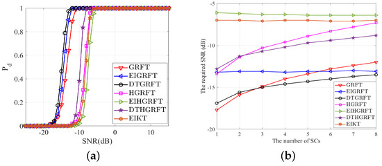
Figure 14. The comparison results of detection performances of different methods for target 1. (a) The curve of $P_d$ at $L=8$. (b) The curve of demanded SNR.

• When the number of SCs is very small, GRFT still has the best detection performance. As the number of SCs increases, the SNR requirements of GRFT continue to increase and the growth rate is faster than that of DT-GRFT, so the detection performance of DT-GRFT quickly outperforms GRFT. Even when the number of SCs is 8, only some units in the two-dimensional detection window contain SCs. At this time, the detection performance of EI-GRFT is inferior to that of DT-GRFT. Since the first threshold of DT-GRFT can more accurately extract the units with SCs, it will basically not accumulate additional noise.
• Due to the slow rotation of the target, the incident angle of the radar observation target changes very little, and the target echo is fully coherent during the entire integration time. Therefore, the detection performance of GRFT, EI-GRFT and DT-GRFT using full coherent integration between pulses is better than that of HGRFT, EI-HGRFT and DT-HGRFT using mixed integration.
• Although the target has a large acceleration, the projection in the slant-range direction is small, so that the defocusing phenomenon of the echo in the range-Doppler domain is not serious. Hence, the detection performance of EI-KT is slightly better than that of EI-HGRFT with too many non-coherent integration times between sub-apertures.

As for target 2, according to its rotation parameters, we can calculate that the echo decoherence time is about 0.04 s, so target 2 represents the situation where the echo decoherence phenomenon occurs. Since target 2 occupies 64 range units, and the part projected onto the same range unit is regarded as one SC, and the number of SCs is set to 1∼ 64. When the number of SCs is 64, the detection curves of different methods are shown in Figure 15a; the demanded SNR under different extracted numbers of SCs are shown in Figure 15b. Similarly, according to Figure 15a,b, we can find that:

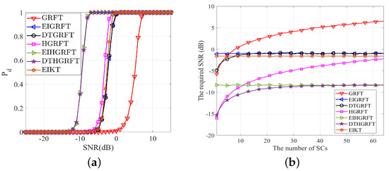
Figure 15. The comparison results of detection performances of different methods for target 2. (a) The curve of $P_d$ at $L=64$. (b) The curve of demanded SNR.

• The faster rotation of the target results in shorter echo dereferencing time, ence the detection performance of the three methods using hybrid integration between pulses is correspondingly better than that of the three methods using full coherent integration.
• The echo decoherence phenomenon causes the performance of EI-GRFT to be slightly worse than that of EI-KT which cannot compensate acceleration.

Specifically, the steps for the seven different techniques, i.e., the GRFT, EI-GRFT, HGRFT, EI-HGRFT, DT-GRFT, DT-HGRFT and EI-KT have been summarized, as shown in Table 3.

Table 3. Summarization of the steps for different methods.

Method	Steps
	Step 1: Confirm the motion model and the order of motion model Step 2: Taking uniformly accelerated motion as an example, divide the grid of search distance R, velocity V, and acceleration A; Step 3: Calculate ${\int }_{-T/2}^{T/2}{s}_{rc}(t_r,t)\times \delta \left[t_r-\frac{2(R+Vt+1/2A{t}^2)}{c}\right]\times exp\left[j4\pi \frac{R+Vt+1/2A{t}^2}{\lambda }\right]dt$,for each distance, speed, and acceleration, where $t_r$ denotes fast time, t denotes slow time, T denotes the accumulation time and $s_{r}c\left(t\right)$ denotes the signal after range compression.
EI-GRFT	Step 1: Calculate GRFT and square the modulus of the result; Step 2: The result obtained in Step 1 is convolutionally processed with a multi-dimensional rectangular window.
HGRFT	Step 1: Confirm the number of sub-apertures and divide sub-apertures; Step 2: Perform GRFT within each sub-aperture (zero time set to the center of the entire echo); Step 3: Conduct noncoherent accumulation between sub-apertures.
EI-HGRFT	Step 1: Calculate HGRFT Step 2: The result obtained in Step 1 is convolutionally processed with a multi-dimensional rectangular window.
DT-GRFT	Step 1: Calculate GRFT and square the modulus of the result; Step2: For the result obtained in Step 1, the original value that exceeds the first threshold is retained, and the value that does not exceed the first threshold is set to 0; Step3: The result obtained in Step 2 is convolutionally processed with a multi-dimensional rectangular window.
DT-HGRFT	Step1: Calculate HGRFT; Step 2: For the result obtained in Step 1, the original value that exceeds the first threshold is retained, and the value that does not exceed the first threshold is set to 0; Step 3: The result obtained in Step 2 is convolutionally processed with a multi-dimensional rectangular window.
EI-KT	Step1: Perform Fourier transform along the fast time dimension to transform the echo into the fast time frequency domain; Step2: Perform scale operation on each fast time frequency unit along the slow time dimension; Step3: Perform inverse Fourier transform along the fast time dimension to transform the echo into a two-dimensional time domain; Step4: Perform Fourier transform along the slow time dimension and take the modulus square; Step5: The result obtained in Step 4 is convolved with a two-dimensional rectangular window.

6.4. Real Data Experiments

To further validate the effectiveness of the proposed methods when applied to realistic applications, we will conduct the real data experiments in this subsection. Stepped-frequency radar is used in the real data experiments, the scenario is shown in Figure 16, and the related parameters are shown in Table 4. As shown in Figure 16, the target is a civil airplane, and its length is much larger than the range resolution, so it has obvious spread phenomenon, which is suitable for the verification of our proposed methods. Note that manually adjustment is adopted to control the radar pointing during the real data experiments to ensure that the target is within the beam.

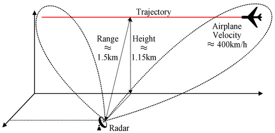
Figure 16. Schematic depiction of the real data scenario.

Table 4. Experimental Parameters and Processing Parameters of Real Data.

Parameters	Values
Waveband	S
Synthetic bandwidth	320 MHz
Synthetic pulse repetition time	4.096 ms
Integration time	0.4096 s
Number of sub-apertures	4
Detection window size of EI/DT-GRFT	$40\times 8$
Detection window size of EI/DT-HGRFT	$40\times 2$
Detection window size of EI-KT	$40\times 16$
The first threshold factor of DT-GRFT	0.5
The first threshold factor of DT-HGRFT	0.6
The first threshold factor of two DT-GRFT joint detection	0, 1
The first threshold factor of two DT-HGRFT joint detection	0, 1.2

Figure 17 shows the pulse-compressed echoes and the range-velocity slices of GRFT and HGRFT in the first integration time of the measured data. It can be seen that the target spreads in both range and velocity dimensions. In addition, although the echo SNR is high, the performance of different methods cannot be judged directly from the integrated amplitude. Thus, Gaussian noise is superimposed on the measured echo in this subsection, and different methods are then used to process the low-SNR data. The obtained results are shown in Figure 18 to Figure 19, and the maximum detection range of different methods is summarized in Table 5. Moreover, the computation time of EI-GRFT, EI-HGRFT, DT-GRFT, DT-HGRFT, twice DT-GRFT joint detection and twice DT-HGRFT joint detection are shown in Table 5 as well. Note that for practical applications, faster hardware (digital signal processor or graphics processing unit), more efficient programing language and 32-bit float data can be used to further reduce the time cost.

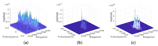
Figure 17. The range-velocity slices of GRFT and HGRFT for real data (a) Echo after pulse compression. (b) The range-velocity slice of GRFT. (c) The range-velocity slice of HGRFT.

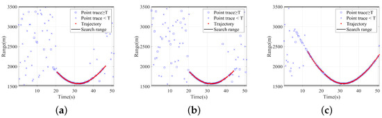
Figure 18. The GRFT, HGRFT and EI-KT results for real data. (a) The GRFT result. (b) The HGRFT result. (c) The EI-KT result.

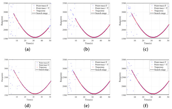
Figure 19. The results of real data under EI-GRFT, EI-HGRFT, DT-GRFT, DT-HGRFT, twice DT-GRFT joint detection and twice DT-HGRFT joint detection. (a) The result of EI-GRFT. (b) The result of EI-HGRFT. (c) The result of DT-GRFT. (d) The result of DT-HGRFT. (e) The result of twice DT-GRFT joint detection. (f) The result of twice DT-HGRFT joint detection.

Table 5. Target Parameters & Processing Parameters.

Methods	Maximum Detection Range	Multiple of Improved Detection Range (GRFT Results Are Benchmarks)	Improved SNR	Total Calculation Time
GRFT	1858 m	-	-	9915 s
HGRFT	1859 m	1.00	0.01	659 s
EI-KT	2369 m	1.28	4.22	601 s
EI-GRFT	2902 m	1.56	7.75	12,983 s
EI-HGRFT	2901 m	1.42	6.04	13,819 s
DT-GRFT	2901 m	1.56	7.74	865 s
DT-HGRFT	2902 m	1.56	7.75	887 s
Two DT-GRFT joint detection	2832 m	1.52	7.32	22,217 s
Two DT-HGRFT joint detection	2901 m	1.56	7.74	1057 s

Due to the low acceleration of the measured target, a certain defocus phenomenon will occur in the integrated of EI-KT. However, the loss of detection capability is negligible. Moreover, the distribution of target SCs is quite dense, so the detection performance of the energy integrated methods and the double-threshold methods are comparable.

In a word, the maximum detection range of the proposed methods are greater than that of GRFT, HGRFT and EI-KT for multi-dimensional spread target detection, which verifies that the proposed methods have better detection performance.

7. Conclusions

In this paper, we conducted a study to achieve high detection performance for multi-dimensional spread target detection with ARDU phenomenon. The study involved analyses of the multi-dimensional spread characteristics, research on long-term integration methods and performance, simulation and real data verification. The main contributions and conclusions are as follows.

First, to address the issue of range spread cross-unit target detection, we proposed the EI-GRFT method while analyzing the echo model of range spread cross-unit targets. Furthermore, we derived the EI-GRFT of spread cross-unit targets which substantially enhances the detection performance.

Subsequently, to solve the problem of multi-dimensional spread cross-unit target detection, we developed the DT-HGRFT method. Our simulations and real data validations demonstrate that DT-HGRFT has better detection performance compared to conventional methods. Also, we presented a multiple DT-HGRFT joint detection method, which resolves the problem of optimizing the first threshold when the number of scattering centers is unknown or the distribution range is large.

In future research, for targets that can be observed continuously, we intend to construct shape and scattering models. These models will produce echoes for coherent integration of spread targets that result in further enhanced detection performance.

References

- Qian, L.C. Research on Radar Target Detection Algorithm Based on Long Time Coherent Integration. Ph.D. Thesis, Air Force Early Warning Academy, Wuhan, China, 2013. [Google Scholar]
- Zhou, X. Research on Key Technologies of Radar Detection for High-Speed and High-Mobility Stealth Targets. Ph.D. Thesis, Beijing Institute of Technology, Beijing, China, 2018. [Google Scholar]
- Richards, M.A. Fundamentals of Radar Signal Processing, 2nd ed.; MCGraw-Hill Education: New York, NY, USA, 2014. [Google Scholar]
- Xu, J.; Yu, J.; Peng, Y.N.; Xia, X.G. Radon-Fourier Transform for Radar Target Detection (II): Blind Speed Sidelobe Suppression. IEEE Trans. Aerosp. Electron. Syst. 2011, 47, 2473–2489. [Google Scholar] [CrossRef]
- Yu, J.; Xu, J.; Peng, Y.N.; Xia, X.G. Radon-Fourier Transform for Radar Target Detection (III): Optimality and Fast Implementations. IEEE Trans. Aerosp. Electron. Syst. 2012, 48, 991–1004. [Google Scholar] [CrossRef]
- Xu, J.; Peng, Y.N.; Xia, X.G.; Farina, A. Focus-before-detection radar signal processing: Part i—Challenges and methods. IEEE Aerosp. Electron. Syst. Mag. 2017, 32, 48–59. [Google Scholar] [CrossRef]
- Xu, J.; Peng, Y.N.; Xia, X.G.; Long, T.; Mao, E.K. Focus-before-detection radar signal processing: Part ii–recent developments. IEEE Aerosp. Electron. Syst. Mag. 2018, 33, 34–49. [Google Scholar] [CrossRef]
- Xu, J.; Peng, Y.N.; Xia, X.G.; Long, T.; Mao, E. Focus-before-detection Methods for Radar Detection of Near Space High-maneuvering Aircrafts. J. Radar 2017, 6, 230–238. [Google Scholar]
- Jia, X.; Xia, X.G.; Peng, S.B.; Ji, Y.; Peng, Y.N.; Qian, L.C. Radar Maneuvering Target Motion Estimation Based on Generalized Radon-Fourier Transform. IEEE Trans. Signal Process. 2012, 60, 6190–6201. [Google Scholar] [CrossRef]
- Swerling, P. Probability of Detection for Fluctuating Targets. Inf. Theory IRE Trans. 1960, IT-6, 269–308. [Google Scholar] [CrossRef]
- Scholtz, R.A.; Kappl, J.J.; Nahi, N.E. The Detection of Moderately-Fluctuating Rayleigh Targets. IEEE Trans. Aerosp. Electron. Syst. 1976, AES-12, 117–126. [Google Scholar] [CrossRef]
- Zhou, X.; Qian, L.C.; Ding, Z.; Xu, J.; Liu, W.; You, P.J.; Long, T. Radar Detection of Moderately Fluctuating Target Based on Optimal Hybrid Integration Detector. IEEE Trans. Aerosp. Electron. Syst. 2019, 55, 2408–2425. [Google Scholar] [CrossRef]
- Zyl, J.J.V.; Carande, R.E.; Lou, Y.; Miller, T.; Wheeler, K.B. The NASA/JPL Three-frequency Polarimetric Airsar System. In Proceedings of the IGARSS ’92 International Geoscience and Remote Sensing Symposium, Houston, TX, USA, 26–29 May 1992; Volume 1, pp. 649–651. [Google Scholar]
- Horn, R. The DLR airborne SAR project E-SAR. In Proceedings of the IGARSS ’96—1996 International Geoscience and Remote Sensing Symposium, Lincoln, NE, USA, 31 May 1996; Volume 3, pp. 1624–1628. [Google Scholar]
- Born, G.H.; Dunne, J.A.; Lame, D.B. Seasat Mission Overview. Science 1979, 204, 1405–1406. [Google Scholar] [CrossRef]
- Attema, E.; Duchossois, G.; Kohlhammer, G. ERS-1/2 SAR land applications: Overview and main results. In Proceedings of the IGARSS ’98—Sensing and Managing the Environment, 1998 IEEE International Geoscience and Remote Sensing. Symposium Proceedings, (Cat. No.98CH36174), Seattle, WA, USA, 6–10 July 1998; Volume 4, pp. 1796–1798. [Google Scholar]
- Desnos, Y.L.; Buck, C.; Guijarro, J.; Levrini, G.; Suchail, J.L.; Torres, R.; Laur, H.; Closa, J.; Rosich, B. The ENVISAT advanced synthetic aperture radar system. In Proceedings of the IGARSS 2000, IEEE 2000 International Geoscience and Remote Sensing Symposium, Taking the Pulse of the Planet: The Role of Remote Sensing in Managing the Environment, Proceedings (Cat. No.00CH37120), Honolulu, HI, USA, 24–28 July 2000; Volume 3, pp. 1171–1173. [Google Scholar]
- Rosenqvist, A.; Shimada, M.; Chapman, B.D.; McDonald, K.; Grandi, G.D.; Jonsson, H.; Williams, C.L.; Rauste, Y.; Nilsson, M.; Sango, D.; et al. An overview of the JERS-1 SAR Global Boreal Forest Mapping (GBFM) project. In Proceedings of the IGARSS 2004, 2004 IEEE International Geoscience and Remote Sensing Symposium, Anchorage, AK, USA, 20–24 September 2004; Volume 2, pp. 1033–1036. [Google Scholar]
- Mahmood, A. RADARSAT-1 Background Mission for a global SAR coverage. In Proceedings of the IGARSS’97. 1997 IEEE International Geoscience and Remote Sensing Symposium Proceedings, Remote Sensing—A Scientific Vision for Sustainable Development, Singapore, 3–8 August 1997; Volume 3, pp. 1217–1219. [Google Scholar]
- Li, C.; Wang, W.; Wang, P.; Chen, J.; Xu, H.; Yang, W.; Yu, Z.; Sun, B.; Li, J. Status and development trend of spaceborne SAR technology. J. Electron. Inf. Technol. 2016, 38, 229–240. [Google Scholar]
- Avent, R.K.; Shelton, J.D.; Brown, P. The ALCOR C-band imaging radar. IEEE Antennas Propag. Mag. 1996, 38, 16–27. [Google Scholar] [CrossRef]
- Hall, T.D.; Duff, G.; Maciel, L.J. The Space Mission at Kwajalein. Linc. Lab. J. 2012, 19. [Google Scholar]
- Czerwinski, M.G.; Usoff, J.M. Development of the Haystack Ultrawideband Satellite Imaging Radar. Linc. Lab. J. 2014, 21, 28–44. [Google Scholar]
- Stambaugh, J.; Lee, R.; Cantrell, W.H. The 4 GHz Bandwidth Millimeter-Wave Radar. Linc. Lab. J. 2012, 19, 64–76. [Google Scholar]
- Stone, M.L.; Banner, G.P. Radars for the Detection and Tracking of Ballistic Missiles, Satellites, and Planets. Linc. Lab. J. 2000, 12, 217–244. [Google Scholar]
- Merz, K.; Banka, D.; Jehn, R.; Landgraf, M.; Rosebrock, J. Observations of interplanetary meteoroids with TIRA. Planet. Space Sci. 2005, 53, 1121–1134. [Google Scholar] [CrossRef]
- Slade, M.A.; Benner, L.A.M.; Silva, A. Goldstone Solar System Radar Observatory: Earth-Based Planetary Mission Support and Unique Science Results. Proc. IEEE 2011, 99, 757–769. [Google Scholar] [CrossRef]
- Harmon, J.K.; Nolan, M.C.; Husmann, D.I.; Campbell, B.A. Arecibo radar imagery of Mars: The major volcanic provinces. Icarus 2012, 220, 990–1030. [Google Scholar] [CrossRef]
- Harmon, J.K.; Nolan, M.C. Arecibo radar imagery of Mars: II. Chryse–Xanthe, polar caps, and other regions. Icarus 2017, 281, 162–199. [Google Scholar] [CrossRef]
- Harmon, J.K.; Slade, M.A.; Rice, M.S. Radar imagery of Mercury’s putative polar ice: 1999–2005 Arecibo results. Icarus 2011, 211, 37–50. [Google Scholar] [CrossRef]
- Slade, M.A.; Zohar, S.; Jurgens, R.F. Venus—Improved spin vector from Goldstone radar observations. Astron. J. 1990, 100, 1369–1374. [Google Scholar] [CrossRef]
- Nicholson, P.D.; French, R.G.; Campbell, D.B.; Margot, J.L.; Nolan, M.C.; Black, G.J.; Salo, H. Radar imaging of Saturn’s rings. Icarus 2005, 177, 32–62. [Google Scholar] [CrossRef]
- Thompson, T.W.; Campbell, B.A.; Bussey, D.B.J. 50 Years of Arecibo Lunar radar mapping. Ursi Radio Sci. Bull. 2017, 89, 23–35. [Google Scholar]
- Lawrence, K.J.; Benner, L.A.M.; Brozović, M.; Ostro, S.J.; Jao, J.S.; Giorgini, J.D.; Slade, M.A.; Jurgens, R.F.; Nolan, M.C.; Howell, E.S.; et al. Arecibo and Goldstone radar images of near-Earth Asteroid (469896) 2005 WC1. Icarus 2018, 300, 12–20. [Google Scholar] [CrossRef]
- Harmon, J.K.; Nolan, M.C.; Giorgini, J.D.; Howell, E.S. Radar observations of 8P/Tuttle: A contact-binary comet. Icarus 2010, 207, 499–502. [Google Scholar] [CrossRef]
- van der Spek, G.A. Detection of a Distributed Target. IEEE Trans. Aerosp. Electron. Syst. 1971, 7, 922–931. [Google Scholar] [CrossRef]
- Hughes, P.K. A High-Resolution Radar Detection Strategy. IEEE Trans. Aerosp. Electron. Syst. 1983, AES-19, 663–667. [Google Scholar] [CrossRef]
- Gerlach, K.; Steiner, M.J.; Lin, F.C. Detection of a spatially distributed target in white noise. IEEE Signal Process. Lett. 1997, 4, 198–200. [Google Scholar] [CrossRef]
- Meng, X.; Qu, D.; He, Y. CFAR detection of range-extended targets in Gaussian background. Syst. Eng. Electron. Technol. 2005, 27, 1012–1015. [Google Scholar]
- He, Y.; feng Gu, X.; Jian, T.; Zhang, B.; Li, B. A M out of n detector based on scattering density. In Proceedings of the IET International Radar Conference, Guilin, China, 20–22 April 2009; pp. 1–4. [Google Scholar]
- Long, T.; Zheng, L.; Li, Y.; Yang, X. Improved Double Threshold Detector for Spatially Distributed Target. IEICE Trans. Commun. 2012, 95-B, 1475–1478. [Google Scholar] [CrossRef]
- Gu, X.; Jian, T.; He, Y. Dual-threshold CFAR detector for range-extended targets and its performance analysis. J. Electron. Inf. 2012, 34, 6. [Google Scholar]
- Wen, X.; Liu, H.; Wen, X.; Liu, H. Normal distribution test algorithm for range-extended target detection. J. Xidian Univ. 2013, 40, 31–35. [Google Scholar]
- Dai, F.; Liu, H.; Wu, S. A Range Extended Target Detector Based on Sequential Statistics. J. Electron. Inf. 2009. [Google Scholar]
- Mohammadi, M.; Moqiseh, A.; Gheidi, H.; Nayebi, M.M. Noncoherent integration of UWB RADAR signals using the Hough transform. In Proceedings of the 2008 European Radar Conference, Amsterdam, The Netherlands, 30–31 October 2008; pp. 9–12. [Google Scholar]
- sheng Zhang, S.; Zeng, T.; Long, T.; peng Yuan, H. Dim target detection based on keystone transform. In Proceedings of the IEEE International Radar Conference, Arlington, VA, USA, 9–12 May 2005; pp. 889–894. [Google Scholar] [CrossRef]
- Wang, L.; Chen, X. Detection of range spread target with coherent integration. In Proceedings of the IET International Radar Conference, Xi’an, China, 14–16 April 2013; pp. 1–4. [Google Scholar]
- Zhu, H.; Chen, Y.; Wang, N. A novel method of wideband radar signal detection. In Proceedings of the 2014 7th International Congress on Image and Signal Processing, Dalian, China, 14–16 October 2014; pp. 847–851. [Google Scholar]
- wen Xu, S.; Shui, P.; Yan, X.Y. CFAR detection of range-spread target in white Gaussian noise using waveform entropy. Electron. Lett. 2010, 46, 647–649. [Google Scholar]
- Liu, S.; Ding, Z.; Zhou, X.; You, P.J. A Novel Method for Abrupt Motion Change Radar Target Detection Based on Generalized Radon-Fourier Transform. In Proceedings of the 2019 IEEE International Conference on Signal, Information and Data Processing (ICSIDP), Chongqing, China, 11–13 December 2019; pp. 1–5. [Google Scholar]
- Xu, J.; Yu, J.; Peng, Y.N.; Xia, X.G. Radon-Fourier Transform for Radar Target Detection, I: Generalized Doppler Filter Bank. IEEE Trans. Aerosp. Electron. Syst. 2011, 47, 1186–1202. [Google Scholar] [CrossRef]
- Sun, Y.; Zeng, W.; Shi, C.; Wang, X. Adaptive estimation of strong scattering points in range-extended target detection. J. Nav. Acad. Aeronaut. Eng. 2014, 29, 440–444. [Google Scholar]
- Guo, P.; Liu, Z.; Luo, D.; Li, J. Range extended target detection method based on online estimation of strong scattering points. J. Electron. Inf. 2020, 42, 910–916. [Google Scholar]
- He, Y.; Guan, J.; Meng, X. Radar Target Detection and Constant False Alarm Processing; Tsinghua University Press: Beijing, China, 2011. [Google Scholar]
Disclaimer/Publisher’s Note: The statements, opinions and data contained in all publications are solely those of the individual author(s) and contributor(s) and not of MDPI and/or the editor(s). MDPI and/or the editor(s) disclaim responsibility for any injury to people or property resulting from any ideas, methods, instructions or products referred to in the content. |
© 2023 by the authors. Licensee MDPI, Basel, Switzerland. This article is an open access article distributed under the terms and conditions of the Creative Commons Attribution (CC BY) license (https://creativecommons.org/licenses/by/4.0/).