Panoptic SwiftNet: Pyramidal Fusion for Real-Time Panoptic Segmentation

Abstract

Dense panoptic prediction is a key ingredient in many existing applications such as autonomous driving, automated warehouses, or remote sensing. Many of these applications require fast inference over large input resolutions on affordable or even embedded hardware. We proposed to achieve this goal by trading off backbone capacity for multi-scale feature extraction. In comparison with contemporaneous approaches to panoptic segmentation, the main novelties of our method are efficient scale-equivariant feature extraction, cross-scale upsampling through pyramidal fusion and boundary-aware learning of pixel-to-instance assignment. The proposed method is very well suited for remote sensing imagery due to the huge number of pixels in typical city-wide and region-wide datasets. We present panoptic experiments on Cityscapes, Vistas, COCO, and the BSB-Aerial dataset. Our models outperformed the state-of-the-art on the BSB-Aerial dataset while being able to process more than a hundred 1MPx images per second on an RTX3090 GPU with FP16 precision and TensorRT optimization.

1. Introduction and Related Work

Panoptic segmentation [1] recently emerged as one of the most important recognition tasks in computer vision. It combines object detection [2] and semantic segmentation [3] in a single task. The goal is to assign a semantic class and instance index to each image pixel. Panoptic segmentation finds its applications in a wide variety of fields such as autonomous driving [4], automated warehouses, smart agriculture [5], and remote sensing [6]. Many of these applications require efficient inference in order to support timely decisions. However, most of the current state-of-the-art does not meet that requirement. State-of-the-art panoptic approaches [7,8,9,10] are usually based on high-capacity backbones in order to ensure a large receptive field, which is required for accurate recognition in large-resolution images. Some of them are based on instance segmentation approaches and therefore require complex post-processing in order to fuse instance-level detections with pixel-level classification [7,8].

Different to all previous approaches to panoptic segmentation, we proposed to leverage multi-scale convolutional representations [11,12] in order to increase the receptive field, and decrease pressure on the backbone capacity through scale equivariance [13]. In simple words, coarse input resolution may provide a more appropriate view of large objects. Furthermore, a mix of features from different scales is both semantically rich and positionally accurate. This allows our model to achieve competitive recognition performance and real-time inference on megapixel resolutions.

Early work on joint semantic and instance segmentation evaluated model performance separately, on both of the two tasks [14,15]. The field gained much attention with the emergence of a unified task called panoptic segmentation and the corresponding metric–panoptic quality [1]. This offered an easy transition path due to straight-forward upgrade of the annotations: panoptic segmentation labels can often be created by combining existing semantic and instance segmentation ground truth. Thus, many popular recognition datasets [16,17,18] were able to release panoptic supervision in a short amount of time, which facilitated further research.

Most of the recent panoptic segmentation methods fall under one of two categories: box-based (or top-down) and box-free (also known as bottom-up) methods. Box-based methods predict the bounding box of the instance and the corresponding segmentation mask [7,8,19]. Usually, semantic segmentation of stuff classes is predicted by a parallel branch of the model. The two branches have to be fused in order to produce panoptic predictions. Panoptic FPN [7] extends the popular Mask R-CNN [20] with a semantic segmentation branch dedicated to the stuff classes. Their fusion module favors instance predictions in pixels where both branches predict a valid class. Concurrent work [8] followed a similar extension idea but proposed a different post-processing step. UPSNet [8] stacks all instance segmentation masks and stuff segmentation maps and applies the softmax to determine the instance index and semantic class in each pixel. EfficientPS [19] combines an EfficentNet backbone, with custom upsampling and panoptic fusion. Although it improves the efficiency with respect to [7,19], its inference speed is still far from real-time.

Box-free methods do not detect instances through bounding box regression [21,22,23,24]. Most of these methods group pixels into instances during a post-processing stage. DeeperLab [21] extends a typical semantic segmentation architecture [25] with a class-agnostic instance segmentation branch. This branch detects five keypoints per instance and groups pixels according to multiple range-dependent maps of offset vectors. Panoptic Deeplab [22] outputs a single heatmap of object centers and a dense map of offset vectors which associates each thing pixel with the centroid of the corresponding instance. Panoptic FCN [23] also detects object centers; however, they aggregate instance pixels through regressed per-instance kernels. Recent approaches [24,26,27] propose unified frameworks for all segmentation tasks, including panoptic segmentation. These frameworks include special transformer-based modules that recover mask-level embeddings and their discriminative predictions. Pixel embeddings are assigned to masks according to the similarity with respect to mask embeddings. This approach seems inappropriate for real-time processing of large images due to the large computational complexity of mask-level recognition.

Semantic segmentation of remote sensing images is a popular and active line of research [28,29,30,31]. On the other hand, only a few papers consider panoptic segmentation of remote sensing images [6,32,33]. Nevertheless, it seems that panoptic segmentation of remote sensing images might support many applications: e.g., automatic compliance assessments of construction work with respect to urban legislation. Just recently, a novel BSB aerial dataset has been proposed [6]. The dataset collected more than 3000 aerial images of urban areas in Brasilia and the accompanying panoptic ground truth. Their experiments involved Panoptic FPN [7] with ResNet-50 and ResNet-101 backbones [34]. In contrast, our method combines multi-scale ResNet-18 [34] features with pyramidal fusion [12], and delivers a better PQ performance and significantly faster inference.

Multi-scale convolutional representations were introduced for semantic segmentation [11]. Further work [12] showed that they can outperform spatial pyramid pooling [35] in terms of effective receptive field. To the best of our knowledge, this is the first work that explored the suitability of multi-scale representations for panoptic segmentation. Similar to [22] our method relies on center and offset prediction for instance segmentation. However, our decoder is shared between instance and semantic segmentation branches. Furthermore, it learns with respect to a boundary-aware objective and aggregates multi-scale features using pyramidal fusion in order to facilitate the recognition of large objects.

The summarized contributions of this work are as follows:

• To the best of our knowledge, this is the first study of multi-scale convolutional representations [11] for panoptic segmentation. We show that pyramidal fusion of multi-scale convolutional representations significantly improves the panoptic segmentation in high-resolution images compared to the single-scale variant;
• We point out that panoptic performance can be significantly improved by training pixel-to-instance assignment through a boundary-aware learning objective;
• Our models outperformed the generalization performance of the previous state-of-the-art in efficient panoptic segmentation [22] while offering around 60% faster inference. Our method achieved a state-of-the-art panoptic performance on the BSB Aerial dataset while being at least 50% faster than previous work [6].

2. Method

Our panoptic segmentation method builds on scale-equivariant features [11], and cross-scale blending through pyramidal fusion [12]. Our models deliver three dense predictions [22]: semantic segmentation, instance centers, and offsets for pixel-to-instance assignment. We attached all three heads to the same latent representation at 4× subsampled resolution. The regressed centers and offsets give rise to class-agnostic instances. Panoptic segmentation maps were recovered by fusing predictions from all three heads [22].

2.1. Upsampling Multi-Scale Features through Pyramidal Fusion

We started from a ResNet-18 backbone [34] and applied it to a three-level image pyramid that involves the original resolution as well as $2\times$ and $4\times$ downsampled resolutions. The resulting multi-scale representation only marginally increases the computational effort with respect to the single-scale baseline. On the other hand, it significantly increases the model’s ability to recognize large objects in high-resolution images. The proposed upsampling path effectively increases the receptive field through cross-scale feature blending, which is also known as pyramidal fusion [12]. Pyramidal fusion proved beneficial for the semantic segmentation performance and we hypothesize that this might be the case for panoptic segmentation as well. In fact, a panoptic model needs to have a look at the whole instance in order to stand a chance to recover the centroid in spite of occlusions and articulated motion. This is hard to achieve when targeting real-time inference on large images since computational complexity is linear in the number of pixels. We conjecture that pyramidal fusion is an efficient way to increase the receptive field and enrich the features with the wider context.

Figure 1 illustrates the resulting architecture. Yellow trapezoids represent residual blocks of a typical backbone which operate on $4\times$, $8\times$, $16\times$ and $32\times$ subsampled resolutions. The trapezoid color indicates feature sharing: the same instance of the backbone was applied to each of the input images. Thus, our architecture complements scale-equivariant feature extraction with scale-aware upsampling. Skip connections from the residual blocks were projected with a single $1\times 1$ convolution (red squares) in order to match the number of channels in the upsampling path. Features from different pyramid levels were combined with elementwise addition (green circles). The upsampling path consisted of five upsampling modules. Each module fused features coming from the backbone via the skip connections and features from the previous upsampling stage. The fusion was performed through elementwise addition and a single $3\times 3$ convolution. Subsequently, the fused features were upsampled by bilinear interpolation. The last upsampling module outputs a feature tensor which is four times subsampled with regard to the input resolution. This feature tensor represents a shared input to the three dense prediction heads that recover the following three tensors: semantic segmentation, centers heatmap, and offset vectors. Each head consisted of a single $1\times 1$ convolution and $4\times$ bilinear upsampling. This design of the prediction heads is significantly faster than in Panoptic Deeplab [22], because it avoids inefficient depthwise-separable convolutions with large kernels on large resolution inputs. Please note that each convolution in the above analysis actually corresponds to a BN-ReLU-Conv unit [36].

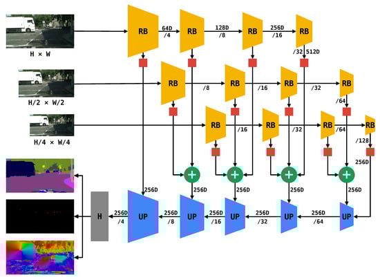
Figure 1. Panoptic SwiftNet with three-way multi-scale feature extraction, pyramidal fusion, common upsampling path, and three prediction heads. Yellow trapezoids denote residual blocks (RB). Red squares represent a $1\times 1$ convolutions that adjust the number of feature maps so that the skip connection can be added to the upsampling stream. Blue trapezoids represent upsampling modules. The gray rectangle represents the three prediction heads. Modules with the same color share parameters. Numbers above the lines (ND) specify the number of channels. Numbers below the lines (/N) specify the downsampling factor with regard to the original resolution of the input image.

The proposed upsampling path has to provide both instance-agnostic features for semantic segmentation as well as instance-aware features for panoptic regression. Consequently, we used 256 channels along the upsampling path, which corresponded to twice the capacity of efficient semantic models [12].

The proposed design differs from the previous work which advocates separate upsampling paths for semantic and instance-specific predictions [22]. Our preliminary validation showed that shared intermediate features can improve panoptic performance when there is enough upsampling capacity.

2.2. Boundary-Aware Learning of Pixel-to-Instance Assignment

Regression of offset centers requires large prediction changes at instance boundaries. A displacement of only one pixel must make a distinction between two completely different instance centers. We conjectured that such abrupt changes require a lot of capacity. Furthermore, it is intuitively clear that the difficulty of offset regression is inversely proportional to the distance from the instance boundary.

Hence, we proposed to prioritize the pixels at instance boundaries by learning offset regression through boundary-aware loss [12,37]. We divided each instance into four regions according to the distance from the boundary. Each of the four regions was assigned a different weight factor. The largest weight factor was assigned to the regions which were closest to the border. The weights diminish as we go towards the interior of the instance. Consequently, we formulated the boundary-aware offset loss as follows:

$$\begin{array}{c}\hfill {\mathcal{L}}_{BAOL}=\frac{1}{H·W}\sum _{i,j}^{H,W}{w}_{i,j}·\left|O_{i,j}-O_{i,j}^{\mathrm{GT}}\right|,w_{i,j}\in \{1,2,4,8\}.\end{array}$$

(1)

In the above equation, H and W represent height and width of the input image, $O_{i,j}$ and $O_{i,j}^{\mathrm{GT}}$ predicted and ground-truth offset vectors at location, and $(i,j)$, and $w_{i,j}$ the boundary-aware weight at the same location.

Note that this is quite different to earlier works [12,37], which are all based on focal loss [38]. To the best of our knowledge, this is the first use of boundary modulation in a learning objective based on L1 regression.

2.3. Compound Learning Objective

We trained our models with the compound loss consisting of three components. The semantic segmentation loss ${\mathcal{L}}_{\mathrm{SEM}}$ is expressed as the usual per-pixel cross entropy [3]. In Cityscapes experiments, we additionally used online hard-pixel mining and considered only the top $20\%$ pixels with the largest loss [25]. The center regression loss ${\mathcal{L}}_{\mathrm{CEN}}$ corresponds to the L2 loss between the predicted centers heatmap and the ground-truth heatmap [22]. This learning objective is common in learning heatmap regression for keypoint detection [39,40]. The offset loss ${\mathcal{L}}_{\mathrm{BAOL}}$ corresponds to the modulated L1 loss as described in (1). The three losses are modulated with hyperparameters ${\lambda }_{\mathrm{SEM}}$, ${\lambda }_{\mathrm{CEN}}$, and ${\lambda }_{\mathrm{BAOL}}$:

$$\begin{array}{c}\hfill \mathcal{L}={\lambda }_{\mathrm{SEM}}·{\mathcal{L}}_{\mathrm{SEM}}+{\lambda }_{\mathrm{CEN}}·{\mathcal{L}}_{\mathrm{CEN}}+{\lambda }_{\mathrm{BAOL}}·{\mathcal{L}}_{\mathrm{BAOL}}.\end{array}$$

(2)

We expressed these hyper-parameters relative to the contribution of the segmentation loss by setting ${\lambda }_{\mathrm{SEM}}=1$. We set ${\lambda }_{\mathrm{CEN}}=200$ in early experiments so that the contribution of the center loss becomes approximately equal to the contribution of the segmentation loss. We validated ${\lambda }_{\mathrm{BAOL}}=0.0025$ in early experiments on the Cityscapes dataset.

Figure 2b shows ground truth targets for a single training example on the BSB Aerial dataset. The semantic segmentation labels associate each pixel with categorical semantic ground truth (top-left). Ground-truth offsets point towards the respective instance centers. Notice abrupt changes at instance-to-instance boundaries (top-right). The ground-truth instance-center heatmap is crafted by Gaussian convolution ($\sigma =5$) of a binary image where ones correspond to instance centers (bottom-left).

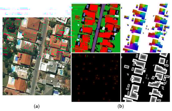
Figure 2. A Panoptic Swiftnet training example consists of an input image (a) and the corresponding ground-truth labels (b): semantic segmentation (top left), offset vectors (top right), heatmap for instance centers (bottom left), and weights for boundary-aware offset loss (bottom right). Offset directions are color coded according to the convention from the previous work in optical flow [41].

We crafted the offset-weight ground-truth by thresholding the distance transform [42] with respect to instance boundaries. Note that pixels at stuff classes do not contribute to the offset loss since the corresponding weights are set to zero (bottom-right).

2.4. Recovering Panoptic Predictions

We recovered panoptic predictions through post-processing of the three model outputs as in Panoptic Deeplab [22]. We first recovered instance centers by non-maximal suppression of the center’s heatmap. Second, each thing pixel was assigned to the closest instance center according to the corresponding displacement from the offset map. Third, each instance was assigned a semantic class by taking arg-max over the corresponding semantic histogram. This voting process presents an opportunity to improve the original semantic predictions, as demonstrated in qualitative experiments. Finally, the panoptic map was constructed by associating instance indices from step 2 with aggregated semantic evidence from step 3.

We greatly improved the execution speed of our Python implementation by implementing custom CUDA modules for steps 3 and 4. Still, the resulting CUDA implementation requires approximately the same time as optimized TensorRT inference in our experiments on Jetson AGX. This suggests that further improvement of the inference speed may require rethinking of the post-processing step.

3. Experiments

We considered multi-scale models with pyramidal fusion based on ResNet-18 [34]. We evaluated the performance of our panoptic models with standard metrics [1]: panoptic quality (PQ), segmentation quality (SQ), and recognition quality (RQ). In some experiments, we also evaluated our panoptic models on semantic and instance segmentation tasks, and show the corresponding performance in terms of mean intersection over union (mIoU) and average precision (AP). For completeness, we now briefly review the used metrics.

Mean intersection over union (mIoU) measures the quality of semantic segmentation. Let $P_c$ and $G_c$ denote all pixels that are predicted and labeled as class c. Then, Equation (3) defines ${\mathrm{IoU}}_c$ as the ratio between the intersection and the union of $P_c$ and $G_c$. This ratio is also known as the Jaccard index. Finally, the mIoU metric is simply an average over all classes $\mathcal{C}$.

$$\begin{array}{c}\hfill {\mathrm{IoU}}_c=\frac{|P_c\cap G_c|}{|P_c\cup G_c|}\mathrm{mIoU}=\frac{{\sum }_{c\in \mathcal{C}}{\mathrm{IoU}}_c}{\left|\mathcal{C}\right|}.\end{array}$$

(3)

Panoptic quality (PQ) measures the similarity between the predicted and the ground truth panoptic segments [1]. Each panoptic segment collects all pixels labeled with the same semantic class and instance index. As in intersection over union, PQ is first computed for each class separately, and then averaged over all classes. In order to compute the panoptic quality, we first needed to match each ground truth segment g with the predicted segment p. The segments were matched if they overlap with $\mathrm{IoU}>0.5$. Thus, matched predicted segments were considered as true positives (TP), unmatched predicted segments as false positives (FP), and unmatched ground truth segments as false negatives (FN). Equation (4) shows that PQ is proportional to the average IoU of true positives, and inversely proportional to the number of false positives and false negatives.

$$\begin{array}{c}\hfill \mathrm{PQ}=\frac{{\sum }_{(p,g)\in \mathit{TP}}\mathrm{IoU}(p,g)}{\left|\mathit{TP}\right|+\frac{1}{2}\left|\mathit{FP}\right|+\frac{1}{2}\left|\mathit{FN}\right|}.\end{array}$$

(4)

PQ can be further factorized into segmentation quality (SQ) and recognition quality (RQ) [1]. This can be achieved by multiplying Equation (4) with $\frac{\left|\mathit{TP}\right|}{\left|\mathit{TP}\right|}$ as shown in Equation (5). The equation clearly indicates that the segmentation quality corresponds to the average IoU of the true positive segment pairs, while the recognition quality corresponds to the F1 score of segment detection for the particular class.

$$\begin{array}{c}\hfill \mathrm{PQ}=\underset{\mathrm{segmentation}\mathrm{quality}\left(\mathrm{SQ}\right)}{\underbrace{\frac{{\sum }_{(p,g)\in \mathit{TP}}\mathrm{IoU}(p,g)}{\phantom{\frac{1}{2}}\left|\mathit{TP}\right|}}}\times \underset{\mathrm{recognition}\mathrm{quality}\left(\mathrm{RQ}\right)}{\underbrace{\frac{\left|\mathit{TP}\right|}{\left|\mathit{TP}\right|+\frac{1}{2}\left|\mathit{FP}\right|+\frac{1}{2}\left|\mathit{FN}\right|}}}.\end{array}$$

(5)

Finally, we briefly recap the average precision (AP) for instance segmentation. In recent years, this name has become a synonym for COCO mean average precision [17]. This metric averages the traditional AP over all possible classes and 10 different IoU thresholds (from 0.5 to 0.95). In order to compute the traditional AP, each instance prediction needs to be associated with a prediction score. The AP measures the quality of ranking induced by the prediction score. It is then computed as the area under the precision-recall curve, which is obtained by considering all possible thresholds of the prediction score. Each prediction is considered a true positive if it overlaps some ground truth instance more than the selected IoU threshold.

Our extensive experimental study considered four different datasets. We first presented our results on the BSB Aerial dataset [6], which collects aerial images. Then, we evaluated our models on two road-driving datasets with high-resolution images: Cityscapes [16] and Mapillary Vistas [18]. Finally, we presented an evaluation on the COCO dataset [17], which gathered a very large number of medium-resolution images from personal collections. Moreover, we provided a validation study of our panoptic model on Cityscapes. We chose Cityscapes for this study because of its appropriate size and high-resolution images which provide a convenient challenge for our pyramidal fusion design. In the end, we measured the inference speed of our models on different GPUs with and without TensorRT optimization.

3.1. BSB Aerial Dataset

The BSB Aerial dataset contains 3000 training, 200 validation, and 200 test images of urban areas in Brasilia, Brazil. All images have the same resolution of $512\times 512$ pixels and are densely labeled with three stuff (street, permeable area, and lake) and eleven thing classes (swimming pool, harbor, vehicle, boat, sports court, soccer field, commercial building, commercial building block, residential building, house, and small construction). The highest number of pixels is annotated as ’permeable area’ because this class considers different types of natural soil and vegetation.

We trained our models for 120,000 iterations on batches consisting of 24 random crops with resolution $512\times 512$ pixels. We used ADAM [43] optimizer with a base learning rate of $3\times {10}^{-4}$ which we polynomially decayed to ${10}^{-7}$. We augmented input images with random scale jitter and horizontal flipping. We also validated image rotation for data augmentation.

Table 1 compares our experimental performance on the BSB Aerial dataset with the related work. Our model based on ResNet-18 outperforms Panoptic FPN with stronger backbones by a large margin. We note improvements over Panoptic FPN with ResNet-50 and ResNet-101 of 5.7 and 4.2 PQ points on the validation data, and 5.9 and 3.1 PQ points on the test data. Besides being more accurate, our model is also significantly faster. In fact, our model is 1.5 times faster than untrained Panoptic-FPN-ResNet-50. Note that we estimated the inference speed of Panoptic FPN with a randomly initialized model which detects less than one instance per image.

Table 1. Performance evaluation of panoptic segmentation methods $512\times 512$ images from the BSB Aerial dataset. FPS denotes frames per second from PyTorch and Python. †—denotes our estimates that measure the inference speed of uninitialized models which on average detect less than 1 instance across the validation dataset.

Model	PQ	SQ	RQ	FPS	GPU
VALIDATION SET
PanopticFPN-R50 [6]	63.8	84.9	74.6	41.3 †	RTX3090
PanopticFPN-R101 [6]	65.3	85.1	76.2	31.8 †	RTX3090
PanopticSwiftNet-RN18 (ours)	69.5	89.3	77.5	64.9	RTX3090
TEST SET
SemSeg-Hybrid [32]	47.4	81.3	58.3	-	-
PanopticFPN-R50 [6]	62.2	85.3	72.2	41.3 †	RTX3090
PanopticFPN-R101 [6]	65.0	85.4	75.5	31.8 †	RTX3090
PanopticSwiftNet-RN18 (ours)	68.1	88.2	76.0	64.9	RTX3090

Image rotation is rarely used for data augmentation on typical road-driving datasets. It makes little sense to encourage the models robustness to rotation if the camera pose is nearly fixed and consistent across all images from both train and validation subsets. However, it seems that rotation in aerial images could simulate other possible poses of the acquisition platform, and thus favor better generalization on test data. Table 2 validates this hypothesis on the BSB aerial dataset. We trained our model in three different setups. The first setup did not use rotation. The second rotated each training example for a randomly chosen angle from the set $\{0^{°},{90}^{°},{180}^{°},{270}^{°}\}$. The third setup rotated each training example for an angle randomly sampled from a range of 0–360$°$. Somewhat surprisingly, the results show that rotated inputs decrease the generalization ability of BSB val. The effect is even stronger when we sampled arbitrary rotations. Visual inspection suggests that this happens due to the constrained acquisition process. In particular, we have noticed that in all inspected images the shadow is pointing at roughly the same direction. We hypothesize that the model learns to use this fact as some sort of orientation landmark for offset prediction. This is similar to road driving scenarios where the models usually learn the bias that the sky covers the top part of the image while the road covers the bottom. Clearly, rotation of the training examples prevents the model from learning these biases, which can hurt the performance on the validation set. The experiments support this hypothesis because the deterioration is much smaller in semantic performance than in panoptic performance. We remind the reader that, unlike panoptic segmentation, semantic segmentation does not require offset predictions.

Table 2. Validation of rotation for data augmentation on the validation set of the BSB Aerial dataset.

Rotation Policy	PQ	SQ	RQ	mIoU
None	69.5	89.3	77.5	75.1
Angle $\in \{0^{°},{90}^{°},{180}^{°},{270}^{°}\}$	68.8	87.8	77.6	74.8
Angle $\in [0^{°},{360}^{°}]$	56.0	86.1	63.9	74.5

Figure 3 shows the predictions of our model on four scenes from BSB Aerial val. The rows show the input image, semantic segmentation, centers heatmap, offset directions, and panoptic segmentation. Panoptic maps designate instances with different shades of the color of the corresponding class.

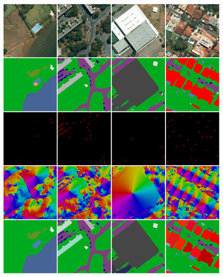
Figure 3. Qualitative results on four scenes from BSB val. Rows show: (first) input image, (second) semantic segmentation, (third) centers heatmap, (fourth) offset directions, and (fifth) panoptic segmentation.

The presented scenes illustrate the diversity of the BSB dataset. We can notice a large green area near the lake (col. 1), but also an urban area with streets and houses (col. 4). There is a great variability in object size. For example, some cars in column 2 are only 10 pixels wide, while the building in column 3 is nearly 400 pixels wide. Our model deals with this variety quite well. We can notice that we correctly detected and segmented most of the cars, and also larger objects such as buildings. However, in the first column we can notice that most of the soccer field in the top-right part of the image is mistakenly segmented as a permeable area. Interestingly, center detection and offset prediction seem quite accurate, but semantic segmentation failed to discriminate between the two classes. This is a fairly common and reasonable mistake because the two classes are visually similar. In the last column, we notice that the road segments are not connected. However, this is caused by the labeling policy which considers trees above the road as a permeable area or unlabeled.

3.2. Cityscapes

The Cityscapes dataset contains 2975 training, 500 validation, and 1525 test images. All images are densely labeled. We trained the models for 90,000 iterations with the ADAM optimizer on $1024\times 2048$ crops with batch size 8. This can be carried out on two GPUs, each with 20 GiB of RAM. We augmented the crops through horizontal flipping and random scaling with a factor between 0.5 and 2.0. As before, we decayed the learning rate from $5\times {10}^{-5}$ to ${10}^{-7}$.

Table 3 compares our panoptic performance and inference speed with other methods from the literature. Panoptic SwiftNet based on ResNet-18 (PSN-RN18) delivers a competitive panoptic performance with respect to models with more capacity, while being significantly faster. In comparison with Panoptic Deeplab [22] based on MobileNet v2, we observed that our method is more accurate in all three subtasks and also faster for $61\%$ when measured in the same runtime environment. We observe that methods based on Mask R-CNN [7,9] achieve poor inference speed and non-competitive semantic segmentation performance in spite of a larger backbone.

Table 3. Panoptic segmentation performance on Cityscapes val. Sections correspond to top-down methods based on Mask R-CNN (top), bottom up methods (middle), and our methods based on pyramidal fusion (bottom). FPS denotes frames per second from PyTorch and Python. FPS* denotes frames per second with FP16 TensorRT optimization. †—denotes our measurements.

Model	PQ	AP	mIoU	FPS	FPS*	GPU
PanopticFPN-RN101 [7]	58.1	33.0	75.7	-	-	-
UPSNet [8]	59.3	33.3	75.2	4.2	-	GTX 1080Ti
SeamLess-RN50 [9]	60.9	33.3	74.9	6.7	-	V100
RTPS-RN50 [10]	58.8	29.0	77.0	10.1	30.3	V100
DeeperLab-WMNv2 [21]	52.2	-	-	4.0	-	V100
PDL-MNv3 [22]	55.4	-	-	15.9	-	V100
PDL-MNv2 [22]	55.1	23.3	75.8	17.8 †	42.2 †	RTX3090
PSN-RN18 (ours)	55.9	26.1	77.2	28.6	61.7	RTX3090

3.3. COCO

The COCO dataset [17] contains digital photographs collected by Flickr users. Images are annotated with 133 semantic categories [44]. The standard split proposes 118,000 images for training, 5000 for validation and 20,000 for testing. We trained for 200,000 iterations with an ADAM optimizer on $640\times 640$ crops with batch size 48. This can be carried out on two GPUs, each with 20 GiB of RAM. We set the learning rate to $4\times {10}^{-4}$ and used polynomial rate decay.

Table 4 presents our results on the COCO validation set. We compared our performance with previous work by evaluating $640\times 640$ crops. We achieved the best accuracy among the methods with real-time execution speed. Although designed for large-resolution images, the pyramidal fusion performs competitively even on COCO images with a median resolution of $640\times 480$ pixels.

Table 4. Panoptic segmentation performance of pyramidal fusion models on COCO val. We do not optimize our models with TensorRT in order to ensure a fair comparison with the previous work. Sections correspond to top-down methods based on Mask R-CNN (top), bottom-up methods (middle), and our method based on pyramidal fusion (bottom).

Model	PQ	PQth	PQst	FPS	GPU
PanopticFPN-RN101 [7]	40.3	47.5	29.5	-	-
RTPS-RN50 [10]	37.1	41.0	31.3	15.9	V100
DeeperLab-WMNv2 [21]	28.1	30.8	24.1	12.0	V100
Max-Deeplab-S [24]	48.4	53.0	41.5	14.9	V100
PanopticFCN-RN50 [23]	42.8	47.9	35.1	16.8	V100
PDL-MNV3 [22]	30.0	-	-	26.3	V100
PSN-RN18 (ours)	30.5	32.1	28.1	64.5	RTX3090

3.4. Mapillary Vistas

The Mapillary Vistas dataset [18] collects high-resolution images of road driving scenes taken under a wide variety of conditions. It contains 18,000 train, 2000 validation and 5000 test images, densely labeled with 65 semantic categories. We trained for 200,000 iterations with an ADAM optimizer. We increased the training speed with respect to the Cityscapes configuration by reducing the crop size to $1024\times 1024$ and increasing the batch size to 16. We composed the training batches by over-sampling crops of rare classes. During evaluation, we resized the input image so that the longer side was equal to 2048 pixels while maintaining the original aspect ratio [22]. Similarly, during training we randomly resized the input image so that the mean resolution was the same as in the evaluation.

Table 5 presents the performance evaluation on Vistas val. Our model achieves comparable accuracy with regard to the literature, while being much faster. These models are slower than their Cityscapes counterparts from Table 3 for two reasons. First, the average resolution of Vistas images in our training and evaluation experiments is $1536\times 2048$ while the Cityscapes resolution is $1024\times 2048$. Second, these models also have slower classification and post-processing steps due to larger numbers of classes and instances.

Table 5. Panoptic segmentation performance of pyramidal fusion model on Mapillary Vistas val. We report average FPS over all validation images.

Model	PQ	mIoU	FPS	GPU
DeeperLab-WMNV2 [21]	22.4	/	3.3	V100
PDL-MNv3 [22]	28.8	/	6.8	V100
PDL-RN50 [22]	33.3	/	3.5	V100
PSN-RN18 (ours)	28.6	47.8	17.0	RTX3090

3.5. Qualitative Experiments

Figure 4 shows the qualitative results on three scenes from validation sets of Cityscapes, Mapillary Vistas and COCO. The rows show the input image, semantic segmentation, centers heatmap, offset directions and the panoptic segmentation. Column 1 shows a Cityscapes scene with a large truck on the left. Semantic segmentation mistakenly recognizes a blob of pixels in the bottom-left as class bus instead of class truck. However, the panoptic map shows that the post-processing step succeeds in correcting the mistake since the correct predictions outvoted the incorrect ones. Hence, the instance segmentation of the truck was completely correct. Column 2 shows a scene from Mapillary Vistas. We observed that our model succeeds in correctly differentiating all distinct instances. Column 3 shows a scene from COCO val. By looking at the offset predictions, we can notice that the model hallucinates an object in the top-right part. However, this does not affect the panoptic segmentation because that part of the scene is classified as the sky (stuff class) in semantic segmentation. Thus, the offset predictions in these pixels are not even considered.

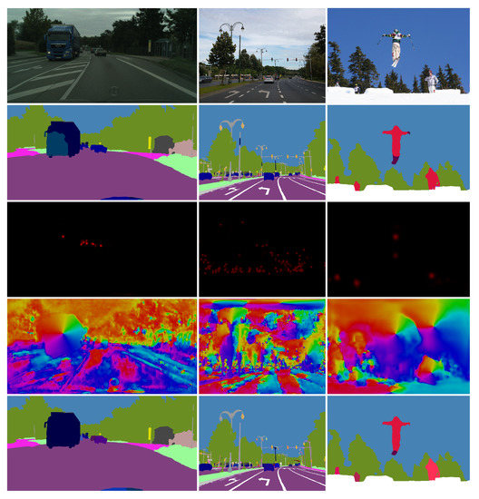
Figure 4. Qualitative results on three scenes from Cityscapes, Mapillary Vistas and COCO. Rows show: (first) input image, (second) semantic segmentation, (third) centers heatmap, (fourth) offset directions, and (fifth) panoptic segmentation.

Figure 5 presents a comparison between our predictions and those of the box-based Panoptic-FPN-R101.

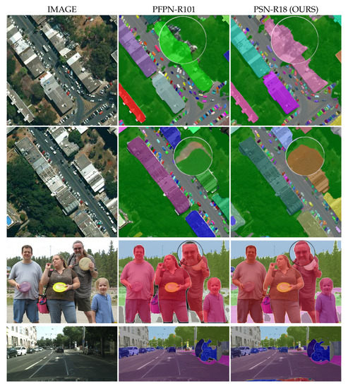
Figure 5. Qualitative comparison between our method (column 3) and Panoptic FPN (column 2) on BSB Aerial dataset (rows 1 and 2), COCO (row 3), and Cityscapes (row 4) [6,7].

The rows show two scenes from the BSB Aerial dataset and one scene each from COCO and Cityscapes. The columns present the input image alongside the corresponding panoptic predictions. We zoomed in on onto circular image regions where the differences between the two models are the most significant. The figure reveals that our model produces more accurate instance masks on larger objects. Conversely, Panoptic FPN often misclassifies boundary pixels as the background instead of a part of the instance. This is likely due to generating instance segmentation masks on a small, fixed-size grid [20]. In contrast, our pixel-to-instance assignments were trained on a fine resolution with a boundary-aware objective. We also observe that our model sometimes merges clusters of small instances in the distance. We believe this is because of the center-point-based object detection and corresponding non-maximum suppression. Box-based approaches perform better in such scenarios, which is consistent with the AP evaluation in Table 3.

3.6. Validation Study on the Cityscapes Dataset

This study quantified the contribution of pyramidal fusion and boundary-aware offset loss to panoptic segmentation accuracy. Table 6 compares pyramidal fusion with spatial pyramid pooling [35,45] as alternatives for providing global context. We trained three separate models with 1, 2, and 3 levels of pyramidal fusion, as well as a single-scale model with spatial pyramidal pooling of $32\times$ subsampled features [43,44,45]. We observed that spatial pyramid pooling improves AP and mIoU by almost four percentage points (cf. rows 1 and 2). This indicates that standard models are unable to capture global context due to an undersized receptive field. This is likely exacerbated by the fact that we initialized with the parameters obtained by training on $224\times 224$ ImageNet images. We note that two-level pyramidal fusion outperforms the SPP model across all metrics. Three-level pyramid fusion achieves further improvements across all metrics. PYRx3 outperforms PYRx2 for 1 PQ point, 2.8 AP points, and 1.1 mIoU points.

Table 6. Comparison of pyramidal fusion with spatial pyramid pooling [35] on Cityscapes val. Both PYRx1 and SPP models operate on single resolution and hence can not exploit pyramidal fusion. The SPP model applies spatial pyramid pooling to $32\times$ subsampled abstract features at the far end of the backbone [45].

Method	PQ	SQ	RQ	AP	mIoU	FPS
PSN-RN18 single	51.7	78.4	64.3	18.7	71.2	34.5
PSN-RN18 SPP	53.5	78.8	66.3	22.4	75.1	32.2
PSN-RN18 PYRx2	54.9	79.2	67.8	23.3	76.1	30.3
PSN-RN18 PYRx3	55.9	79.5	68.9	26.1	77.2	28.6

Table 7 explores the upper performance bounds with regard to particular model outputs. These experiments indicate that semantic segmentation represents the most important challenge to achieving accurate panoptic segmentation. Perfect semantic segmentation improves panoptic quality by roughly 20 points. However, we believe that rapid progress in semantic segmentation accuracy is not very likely due to the wide popularity of the problem. When comparing the oracle center and oracle offsets, we observed that the latter brings significantly larger improvements: 3 PQ and 10 AP points over the regular model. In early experiments, most of the offset errors were located at instance boundaries, so we introduced the boundary-aware offset loss (1).

Table 7. Evaluation of models with different oracle components. Labels +GT X denote models which use ground truth information for the prediction X. Note that c&o denotes centers and offsets.

Model	PQ	SQ	RQ	AP	mIoU
PSN-RN18	55.9	79.5	68.9	26.1	77.2
+GT semseg	76.2	91.0	82.5	39.6	100.0
+GT centers	56.9	79.5	70.1	22.9	77.2
+GT offsets	59.1	83.0	70.4	36.8	77.2
+GT c&o	61.6	83.3	73.2	38.2	77.2

Table 8 explores the influence of the boundary-aware offset loss (1) on the PSN-18 accuracy. We considered three variants based on the number of regions that divide each instance. In each variant, we set the largest weight equal to eight for the region closest to the border, and then gradually reduce it to one for the most distant region. Note that we set the overall weight of the offset loss to $\lambda =0.01$ when we did not use the the boundary-aware Formulation (1). We observed that the boundary-aware loss with four regions per instance brings noticeable improvements across all metrics. The largest improvement is in instance segmentation performance, which increases by 1.1 AP points.

Table 8. Validation of boundary-aware offset loss for the PSN-RN18 PYRx3 model on Cityscapes val. The presented results are average over two runs.

Offset Loss	PQ	SQ	RQ	AP	mIoU
L1	55.2	79.2	68.2	25.2	76.3
L1-BAL (3 regions per instance)	55.2	79.2	68.2	25.5	76.6
L1-BAL (4 regions per instance)	55.9	79.5	68.9	26.3	76.6
L1-BAL (8 regions per instance)	55.5	79.3	68.5	25.2	76.8

3.7. Inference Speed after TensorRT Optimization

Figure 6 evaluates the speed of our optimized models across different input resolutions. All models were run from Python within the TensorRT execution engine. We used TensorRT to optimize the same model for two graphics cards and two precisions (FP16 and FP32). Note, however, that these optimizations involved only the network inference, while the post-processing step was executed with a combination of Pytorch [46] and cupy [47].

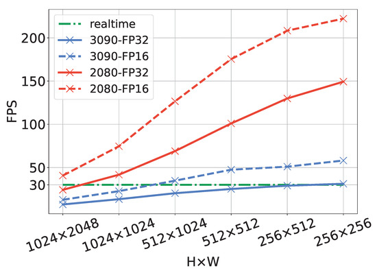
Figure 6. Inference speed of a three-level PSN-RN18 across different input resolutions for two graphics cards and two precisions. All configurations involve the same model after optimizing it with TensorRT. All datapoints are averaged over all images from Cityscapes val in order to account for the dependence of the post-processing time on scene complexity.

Interestingly, FP16 brings almost a $2\times$ improvement across all experiments, although RTX3090 declares the same peak performance for FP16 and FP32. This suggests that it is likely that our performance bottleneck corresponds to memory bandwidth rather than computing power.

We started the clock when an image was synchronized in CUDA memory and stopped it when the post-processing was completed. We captured realistic post-processing times by expressing all datapoints as average inference speed over all images from Cityscapes val. The figure shows that our model achieves real-time inference speed even on high-resolution 2MPx images. Our PSN-RN18 model achieves more than 100 FPS on 1MPx resolution with FP16 RTX3090.

4. Conclusions

We have proposed a novel panoptic architecture based on multi-scale features, cross-scale blending, and bottom-up instance recognition. Ablation experiments indicate clear advantages of the multi-scale architectures and boundary-aware learning for the panoptic performance. Experiments with oracle components suggest that semantic segmentation represents a critical ingredient of panoptic performance. Panoptic SwiftNet-RN18 achieves a state-of-the-art generalization performance and the fastest inference on the BSB Aerial dataset. The proposed method is especially appropriate for remote sensing applications as it is able to efficiently process very large resolution inputs. It also achieves a state-of-the-art performance on Cityscapes as well as a competitive performance on Vistas and COCO, compared with all models aiming at real-time inference. The source code will be publicly available upon acceptance.

References

- Kirillov, A.; He, K.; Girshick, R.; Rother, C.; Dollár, P. Panoptic segmentation. In Proceedings of the IEEE/CVF Conference on Computer Vision and Pattern Recognition, Long Beach, CA, USA, 15–20 June 2019; pp. 9404–9413. [Google Scholar]
- Ren, S.; He, K.; Girshick, R.; Sun, J. Faster r-cnn: Towards real-time object detection with region proposal networks. Adv. Neural Inf. Process. Syst. 2015, 28, 1497. [Google Scholar] [CrossRef] [PubMed]
- Long, J.; Shelhamer, E.; Darrell, T. Fully convolutional networks for semantic segmentation. In Proceedings of the IEEE Conference on Computer Vision and Pattern Recognition, Boston, MA, USA, 7–12 June 2015; pp. 3431–3440. [Google Scholar]
- Zendel, O.; Schörghuber, M.; Rainer, B.; Murschitz, M.; Beleznai, C. Unifying panoptic segmentation for autonomous driving. In Proceedings of the IEEE/CVF Conference on Computer Vision and Pattern Recognition, New Orleans, LA, USA, 18–24 June 2022; pp. 21351–21360. [Google Scholar]
- Garnot, V.S.F.; Landrieu, L. Panoptic segmentation of satellite image time series with convolutional temporal attention networks. In Proceedings of the IEEE/CVF International Conference on Computer Vision, Montreal, BC, Canada, 11–17 Qctober 2021; pp. 4872–4881. [Google Scholar]
- De Carvalho, O.L.F.; de Carvalho Júnior, O.A.; Silva, C.R.E.; de Albuquerque, A.O.; Santana, N.C.; Borges, D.L.; Gomes, R.A.T.; Guimarães, R.F. Panoptic segmentation meets remote sensing. Remote Sens. 2022, 14, 965. [Google Scholar] [CrossRef]
- Kirillov, A.; Girshick, R.; He, K.; Dollár, P. Panoptic feature pyramid networks. In Proceedings of the EEE/CVF Conference on Computer Vision and Pattern Recognition, Long Beach, CA, USA, 15–20 June 2019; pp. 6399–6408. [Google Scholar]
- Xiong, Y.; Liao, R.; Zhao, H.; Hu, R.; Bai, M.; Yumer, E.; Urtasun, R. Upsnet: A unified panoptic segmentation network. In Proceedings of the IEEE/CVF Conference on Computer Vision and Pattern Recognition, Long Beach, CA, USA, 15–20 June 2019; pp. 8818–8826. [Google Scholar]
- Porzi, L.; Bulo, S.R.; Colovic, A.; Kontschieder, P. Seamless Scene Segmentation. In Proceedings of the IEEE/CVF Conference on Computer Vision and Pattern Recognition (CVPR), Long Beach, CA, USA, 15–20 June 2019. [Google Scholar]
- Hou, R.; Li, J.; Bhargava, A.; Raventos, A.; Guizilini, V.; Fang, C.; Lynch, J.; Gaidon, A. Real-Time Panoptic Segmentation From Dense Detections. In Proceedings of the IEEE/CVF Conference on Computer Vision and Pattern Recognition (CVPR), Seattle, DC, USA, 14–19 June 2020. [Google Scholar]
- Farabet, C.; Couprie, C.; Najman, L.; LeCun, Y. Learning hierarchical features for scene labeling. IEEE Trans. Pattern Anal. Mach. Intell. 2012, 35, 1915–1929. [Google Scholar] [CrossRef] [PubMed]
- Oršić, M.; Šegvić, S. Efficient semantic segmentation with pyramidal fusion. Pattern Recognit. 2021, 110, 107611. [Google Scholar] [CrossRef]
- Krešo, I.; Čaušević, D.; Krapac, J.; Šegvić, S. Convolutional scale invariance for semantic segmentation. In Proceedings of the German Conference on Pattern Recognition, Hannover, Germany, 27 August 2016; Springer: Cham, Switzerland, 2016; pp. 64–75. [Google Scholar]
- Yao, J.; Fidler, S.; Urtasun, R. Describing the scene as a whole: Joint object detection, scene classification and semantic segmentation. In Proceedings of the 2012 IEEE Conference on Computer Vision and Pattern Recognition, Providence, RI, USA, 16–20 June 2012; IEEE: Piscataway, NJ, USA, 2012; pp. 702–709. [Google Scholar]
- Dvornik, N.; Shmelkov, K.; Mairal, J.; Schmid, C. Blitznet: A real-time deep network for scene understanding. In Proceedings of the IEEE International Conference on Computer Vision, Venice, Italy, 22–29 October 2017; pp. 4154–4162. [Google Scholar]
- Cordts, M.; Omran, M.; Ramos, S.; Rehfeld, T.; Enzweiler, M.; Benenson, R.; Franke, U.; Roth, S.; Schiele, B. The Cityscapes Dataset for Semantic Urban Scene Understanding. In Proceedings of the IEEE Conference on Computer Vision and Pattern Recognition (CVPR), Las Vegas, NA, USA, 27–30 June 2016. [Google Scholar]
- Lin, T.Y.; Maire, M.; Belongie, S.; Hays, J.; Perona, P.; Ramanan, D.; Dollár, P.; Zitnick, C.L. Microsoft coco: Common objects in context. In Proceedings of the European Conference on Computer Vision, Zurich, Switzerland, 6–12 September 2014; Springer: Cham, Switzerland, 2014; pp. 740–755. [Google Scholar]
- Neuhold, G.; Ollmann, T.; Rota Bulo, S.; Kontschieder, P. The mapillary vistas dataset for semantic understanding of street scenes. In Proceedings of the IEEE International Conference on Computer Vision, Venice, Italy, 22–29 October 2017; pp. 4990–4999. [Google Scholar]
- Mohan, R.; Valada, A. Efficientps: Efficient panoptic segmentation. Int. J. Comput. Vis. 2021, 129, 1551–1579. [Google Scholar] [CrossRef]
- He, K.; Gkioxari, G.; Dollár, P.; Girshick, R. Mask r-cnn. In Proceedings of the IEEE International Conference on Computer Vision, Venice, Italy, 22–29 October 2017; pp. 2961–2969. [Google Scholar]
- Yang, T.J.; Collins, M.D.; Zhu, Y.; Hwang, J.J.; Liu, T.; Zhang, X.; Sze, V.; Papandreou, G.; Chen, L.C. Deeperlab: Single-shot image parser. arXiv 2019, arXiv:1902.05093. [Google Scholar]
- Cheng, B.; Collins, M.D.; Zhu, Y.; Liu, T.; Huang, T.S.; Adam, H.; Chen, L.C. Panoptic-DeepLab: A Simple, Strong, and Fast Baseline for Bottom-Up Panoptic Segmentation. In Proceedings of the IEEE/CVF Conference on Computer Vision and Pattern Recognition (CVPR), Seattle, WA, USA, 13–19 June 2020. [Google Scholar]
- Li, Y.; Zhao, H.; Qi, X.; Wang, L.; Li, Z.; Sun, J.; Jia, J. Fully Convolutional Networks for Panoptic Segmentation. In Proceedings of the IEEE/CVF Conference on Computer Vision and Pattern Recognition (CVPR), Nashville, TN, USA, 20–25 June 2021; pp. 214–223. [Google Scholar]
- Wang, H.; Zhu, Y.; Adam, H.; Yuille, A.; Chen, L.C. MaX-DeepLab: End-to-End Panoptic Segmentation with Mask Transformers. In Proceedings of the IEEE/CVF Conference on Computer Vision and Pattern Recognition (CVPR), Nashville, TN, USA, 20–25 June 2021; pp. 5463–5474. [Google Scholar]
- Chen, L.C.; Zhu, Y.; Papandreou, G.; Schroff, F.; Adam, H. Encoder-Decoder with Atrous Separable Convolution for Semantic Image Segmentation. In Proceedings of the ECCV, Munich, Germany, 8–14 September 2018. [Google Scholar]
- Cheng, B.; Schwing, A.; Kirillov, A. Per-pixel classification is not all you need for semantic segmentation. Adv. Neural Inf. Process. Syst. 2021, 34, 17864–17875. [Google Scholar]
- Li, F.; Zhang, H.; Xu, H.; Liu, S. Mask dino: Towards a unified transformer-based framework for object detection and segmentation. arXiv 2022, arXiv:2206.02777. [Google Scholar]
- Xu, Z.; Zhang, W.; Zhang, T.; Li, J. HRCNet: High-resolution context extraction network for semantic segmentation of remote sensing images. Remote Sens. 2020, 13, 71. [Google Scholar] [CrossRef]
- Liu, Y.; Ren, Q.; Geng, J.; Ding, M.; Li, J. Efficient patch-wise semantic segmentation for large-scale remote sensing images. Sensors 2018, 18, 3232. [Google Scholar] [CrossRef] [PubMed]
- Zhang, J.; Lin, S.; Ding, L.; Bruzzone, L. Multi-scale context aggregation for semantic segmentation of remote sensing images. Remote Sens. 2020, 12, 701. [Google Scholar] [CrossRef]
- Li, Z.; Yang, J.; Wang, B.; Li, Y.; Pan, T. Maskformer with Improved Encoder-Decoder Module for Semantic Segmentation of Fine-Resolution Remote Sensing Images. In Proceedings of the 2022 IEEE International Conference on Image Processing (ICIP), Bordeaux, France, 16–19 October 2022; pp. 1971–1975. [Google Scholar] [CrossRef]
- De Carvalho, O.L.; de Carvalho Júnior, O.A.; Anesmar, O.; Santana, N.C.; Borges, D.L. Rethinking panoptic segmentation in remote sensing: A hybrid approach using semantic segmentation and non-learning methods. IEEE Geosci. Remote Sens. Lett. 2022, 19, 3512105. [Google Scholar] [CrossRef]
- Hua, X.; Wang, X.; Rui, T.; Shao, F.; Wang, D. Cascaded panoptic segmentation method for high resolution remote sensing image. Appl. Soft Comput. 2021, 109, 107515. [Google Scholar] [CrossRef]
- He, K.; Zhang, X.; Ren, S.; Sun, J. Deep Residual Learning for Image Recognition. In Proceedings of the IEEE Conference on Computer Vision and Pattern Recognition (CVPR), Las Vegas, NA, USA, 37–30 June 2016. [Google Scholar]
- Zhao, H.; Shi, J.; Qi, X.; Wang, X.; Jia, J. Pyramid scene parsing network. In Proceedings of the IEEE Conference on Computer Vision and Pattern Recognition, Honolulu, HI, USA, 21–26 July 2017; pp. 2881–2890. [Google Scholar]
- He, K.; Zhang, X.; Ren, S.; Sun, J. Identity mappings in deep residual networks. In Proceedings of the Computer Vision–ECCV 2016: 14th European Conference, Amsterdam, The Netherlands, 11–14 October 2016; Springer: Cham, Switzerland, 2016; pp. 630–645. [Google Scholar]
- Zhen, M.; Wang, J.; Zhou, L.; Fang, T.; Quan, L. Learning fully dense neural networks for image semantic segmentation. In Proceedings of the AAAI Conference on Artificial Intelligence, Honolulu, HI, USA, 27 January–1 February 2019; Volume 33, pp. 9283–9290. [Google Scholar]
- Lin, T.Y.; Goyal, P.; Girshick, R.; He, K.; Dollár, P. Focal loss for dense object detection. In Proceedings of the IEEE International Conference on Computer Vision, Venice, Italy, 22–29 October 2017; pp. 2980–2988. [Google Scholar]
- Xiao, B.; Wu, H.; Wei, Y. Simple baselines for human pose estimation and tracking. In Proceedings of the European Conference on Computer Vision (ECCV), Munich, Germany, 8–14 September 2018; pp. 466–481. [Google Scholar]
- Newell, A.; Yang, K.; Deng, J. Stacked hourglass networks for human pose estimation. In Proceedings of the Computer Vision–ECCV 2016: 14th European Conference, Amsterdam, The Netherlands, 11–14 October 2016; Springer: Cham, Switzerland, 2016; pp. 483–499. [Google Scholar]
- Baker, S.; Scharstein, D.; Lewis, J.; Roth, S.; Black, M.J.; Szeliski, R. A database and evaluation methodology for optical flow. Int. J. Comput. Vis. 2011, 92, 1–31. [Google Scholar] [CrossRef]
- Borgefors, G. Distance transformations in digital images. Comput. Vis. Graph. Image Process. 1986, 34, 344–371. [Google Scholar] [CrossRef]
- Kingma, D.P.; Ba, J. Adam: A Method for Stochastic Optimization. In Proceedings of the 3rd International Conference on Learning Representations, ICLR 2015, San Diego, CA, USA, 7–9 May 2015; Bengio, Y., LeCun, Y., Eds.; IEEE: Piscataway, NJ, USA, 2015. [Google Scholar]
- Caesar, H.; Uijlings, J.; Ferrari, V. Coco-stuff: Thing and stuff classes in context. In Proceedings of the IEEE Conference on Computer Vision and Pattern Recognition, Salt Lake City, UT, USA, 18–23 June 2018; pp. 1209–1218. [Google Scholar]
- Krešo, I.; Krapac, J.; Šegvić, S. Efficient ladder-style densenets for semantic segmentation of large images. IEEE Trans. Intell. Transp. Syst. 2020, 22, 4951–4961. [Google Scholar] [CrossRef]
- Paszke, A.; Gross, S.; Massa, F.; Lerer, A.; Bradbury, J.; Chanan, G.; Killeen, T.; Lin, Z.; Gimelshein, N.; Antiga, L.; et al. Pytorch: An imperative style, high-performance deep learning library. Adv. Neural Inf. Process. Syst. 2019, 32, 8026–8037. [Google Scholar]
- Okuta, R.; Unno, Y.; Nishino, D.; Hido, S.; Loomis, C. CuPy: A NumPy-Compatible Library for NVIDIA GPU Calculations. In Proceedings of the Workshop on Machine Learning Systems (LearningSys) in The Thirty-First Annual Conference on Neural Information Processing Systems (NIPS), Long Beach, CA, USA, 4–9 December 2017. [Google Scholar]
Disclaimer/Publisher’s Note: The statements, opinions and data contained in all publications are solely those of the individual author(s) and contributor(s) and not of MDPI and/or the editor(s). MDPI and/or the editor(s) disclaim responsibility for any injury to people or property resulting from any ideas, methods, instructions or products referred to in the content. |
© 2023 by the authors. Licensee MDPI, Basel, Switzerland. This article is an open access article distributed under the terms and conditions of the Creative Commons Attribution (CC BY) license (https://creativecommons.org/licenses/by/4.0/).