Article

Evaluation of Airborne HySpex and Spaceborne PRISMA Hyperspectral Remote Sensing Data for Soil Organic Matter and Carbonates Estimation

1
Laboratory of Remote Sensing, Spectroscopy, and GIS, Department of Agriculture, Aristotle University of Thessaloniki, 54124 Thessaloniki, Greece
2
Helmholtz Center, Potsdam GFZ German Research Centre for Geosciences, Section Remote Sensing and Geoinformatics, 14473 Potsdam, Germany
3
Institute of Soil Science, Leibniz University Hannover, Herrenhäuser Str. 2, 30419 Hannover, Germany
4
Institute of Methodologies for Environmental Analysis (IMAA), National Council of Research (CNR), C. da S. Loja, Tito Scalo, 85050 Potenza, Italy
5
School of Science and Technology, International Hellenic University, 14th km Thessaloniki—N. Moudania, 57001 Thermi, Greece
6
Institute for Space Sciences, Free University Berlin, 12165 Berlin, Germany
7
Centre of Research and Technology—Hellas (CERTH), Institute for Bio—Economy and Agri—Technology (iBO), 57001 Thessaloniki, Greece
*
Author to whom correspondence should be addressed.
Remote Sens. 2023, 15(4), 1106; https://doi.org/10.3390/rs15041106
Submission received: 23 December 2022 / Revised: 5 February 2023 / Accepted: 12 February 2023 / Published: 17 February 2023
(This article belongs to the Special Issue Remote Sensing for Soil Organic Carbon Mapping and Monitoring)

Abstract

:
Remote sensing and soil spectroscopy applications are valuable techniques for soil property estimation. Soil organic matter (SOM) and calcium carbonate are important factors in soil quality, and although organic matter is well studied, calcium carbonates require more investigation. In this study, we validated the performance of laboratory soil spectroscopy for estimating the aforementioned properties with referenced in situ data. We also examined the performance of imaging spectroscopy sensors, such as the airborne HySpex and the spaceborne PRISMA. For this purpose, we applied four commonly used machine learning algorithms and six preprocessing methods for the evaluation of the best fitting algorithm.. The study took place over crop areas of Amyntaio in Northern Greece, where extensive soil sampling was conducted. This is an area with a very variable mineralogical environment (from lignite mine to mountainous area). The SOM results were very good at the laboratory scale and for both remote sensing sensors with R2 = 0.79 for HySpex and R2 = 0.76 for PRISMA. Regarding the calcium carbonate estimations, the remote sensing accuracy was R2 = 0.82 for HySpex and R2 = 0.36 for PRISMA. PRISMA was still in the commissioning phase at the time of the study, and therefore, the acquired image did not cover the whole study area. Accuracies for calcium carbonates may be lower due to the smaller sample size used for the modeling procedure. The results show the potential for using quantitative predictions of SOM and the carbonate content based on soil and imaging spectroscopy at the air and spaceborne scales and for future applications using larger datasets.

1. Introduction

The important role of soil organic matter (SOM) in supporting soil functions has been widely demonstrated [1]. SOM directly benefits soils and plants by sequestering nutrients and water, while a reduction in SOM can lead to soil erosion and structure loss. In recent years, research has focused on the role of SOM, and more specifically on its component soil organic carbon (SOC), SOC contributes to climate change mitigation and adaptation and, subsequently, to the attainment of sustainable development goals (SDGs) [2]. Climate is one of the most important factors that affects SOM, which makes the relationship bidirectional [3]. Carbonate minerals may impact the global carbon cycle, as they are considered one of the largest C reservoirs on Earth [1,4]. Calcium carbonate (CaCO3) is one of the most common carbonate minerals in soils. The physical, chemical, and biological properties of soils are affected by the amount and distribution of carbonates. Carbonates affect soil pH levels, acting as a buffer, and also affect the heavy metal bioavailability [5,6].
Agricultural and environmental applications require knowledge about the soil conditions. However, large soil sampling campaigns can be tedious and expensive tasks. One has to consider the soil properties in question and select a proper soil sampling design that can also be accomplished with the respective budget [7]. The subsequent soil chemical analyses lead to additional costs and can have an environmental impact due to the chemical reagents used. In some cases, the spatial variation of different soil properties occurs at a finer spatial scale than is feasible for soil sampling and laboratory analyses [8]. Therefore, alternative methods are needed to minimize the cost and time needed for soil property estimation. Soil reflectance spectroscopy in the Vis-NIR-SWIR (400–2500 nm) relies on energy matter interactions [9] and has been widely assessed in previous decades. The evolution of sensors in terms of their spectral and spatial resolution has increased the ability to estimate soil properties from local to global scales by using proximal and remote sensing techniques [10,11,12,13].
Soil reflectance spectroscopy is considered an effective way to quantitatively estimate soil properties under laboratory conditions [14,15]. Measurements are acquired under controlled conditions, and while most laboratories use similar protocols to perform them, effort is currently being made to establish a standard protocol. Another advantage of laboratory soil spectroscopy is that the instruments used have a high spectral resolution of approximately 1 nm, which provides information regarding the relationship between soil properties and specific spectral wavelengths. However, this procedure has the disadvantage of a low spatial resolution. In order to generate prediction maps of soil properties from laboratory measurements, one has to apply geostatistical methods, such as kriging interpolation. The use of airborne and spaceborne hyperspectral sensors offers an alternative, highly promising method to generate maps of soil properties at larger spatial scales with a slightly lower spectral resolution than that achieved with laboratory measurements. An extensive amount of literature exists on the prediction of soil properties based on airborne hyperspectral remote sensing [13,16,17,18].
The most important wavelengths for SOM/SOC estimation are located in the visible region around 550–700 nm, in the NIR region around 850 nm, and in the SWIR region from 1700 to 1900 nm and from 2100 to 2400 nm [19]. The accuracy of soil property estimations drops from airborne to spaceborne sensors due to a lower signal-to-noise ratio, a coarser spectral and spatial resolution along with atmospheric effects, and surface disturbing effects (soil roughness, soil moisture, vegetation cover) [18,20]. Despite this, results of studies using airborne and spaceborne sensors are very promising, with accuracies of R2 = 0.85 for the airborne HyMap sensor [21] and R2 = 0.67 for the spaceborne EnMAP sensor [22,23], while simulated EnMAP imagery in a local PLSR approach was shown to perform better with R² = 0.77 [24]
Carbonates have distinctive features, mostly in the SWIR region. When light interacts with carbonates, it is absorbed by vibrational processes in the carbonate ion and water, as well as by electronic processes due to the presence of metal cations. The vibrational processes can produce specific overtone bands in the infrared region. In particular, there are two strong absorption bands near 2300–2350 nm and 2500–2550 nm and weaker absorption bands near 1850–1870 nm, 1970–2000 nm, and 2120–2160 nm [25]. These distinctive absorption features also depend on the particle size and porosity. Studies have shown relative good results with the application of both proximal [26,27,28,29,30] and remote sensing techniques [31].
Important factors affecting the accuracy of the predictions, apart from the number of samples, are the choice of preprocessing method, the data mining algorithm used, and the combination of the two [32]. The partial least squares regression (PLSR) was the most widely used method in early studies and is still preferred today. The use of machine learning algorithms is gaining relevance due to collaborations with scientists in the field of data analytics. These methods have created more accurate results, specifically for large datasets i.e., soil spectral libraries that are created all around the world [33].
In this study, we aim to further demonstrate the usefulness of hyperspectral data at different scales, from laboratory to remote sensing hyperspectral sensors for topsoil SOM and CaCO3 estimation by exploring the potential of new spaceborne sensors, such as PRISMA. This is the first study to evaluate imaging spectroscopy data at both airborne and spaceborne scales from HySpex and PRISMA. We also aim to explore the effects of various preprocessing and data mining algorithms on the model accuracy.

2. Materials and Methods
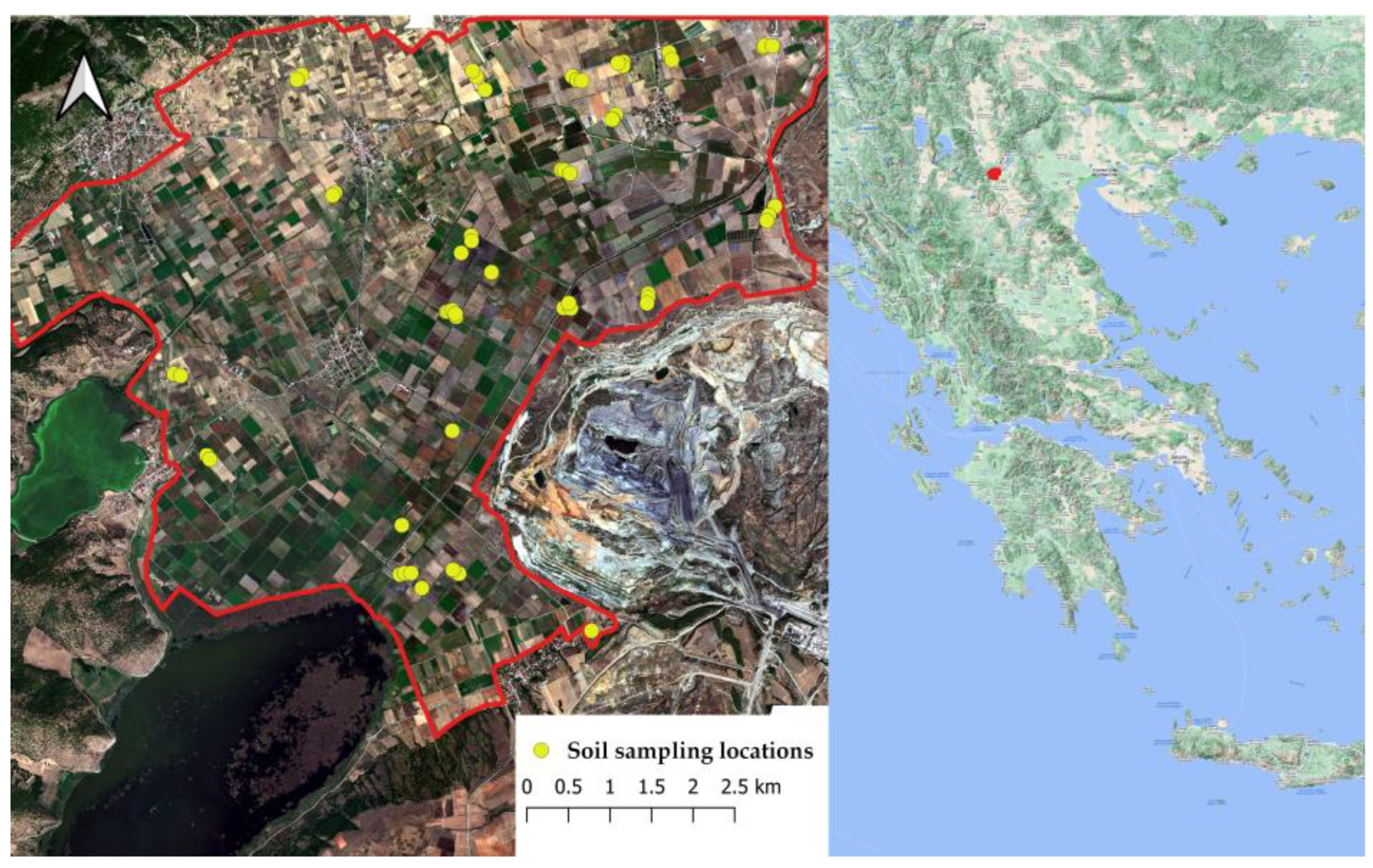
The procedure applied in this study involves four main steps. Firstly, field campaigns were organized in 2018 and 2019 to collect soil samples for chemical analyses. Secondly, laboratory soil spectral measurements were performed under controlled conditions (dark box) with the PSR+ 3500 instrument (Spectral Evolution Inc., Lawrence, MA, USA). Thirdly, airborne hyperspectral imaging with the HySpex sensor from 2019 was used to estimate SOM and CaCO3. Lastly, spaceborne hyperspectral imagery from the PRISMA satellite was used to estimate the aforementioned properties. Model calibration was done using different multivariate regression algorithms (PLSR, Cubist, Random Forest, and Support Vector Machines) and six different preprocessing approaches.

2.1. Study Area

The study area is located in the municipality of Amyntaio in the regional unit of Florina in the region of West Macedonia, Greece at 40°37′59″N 21°34′59″E (Figure 1). The area is 46.10 km2 in size and is mainly agricultural with fields of alfalfa, winter wheat, and corn.
The area is characterized by heterogeneous terrain which is the reason for the high variability in the soil properties in terms of the carbonate and organic matter contents, which range from a very high carbonate content in the northeast to very high organic matter content in the southwest (Figure 2). Soils mainly consist of tertiary and quaternary sediments in the central area and Triassic-Jurassic limestones in the northeast. To the south of the study area there is a Lignite mine, where the Public Power Company of Greece is undergoing intensive mining activity. More information about the area can be also found in [34,35].

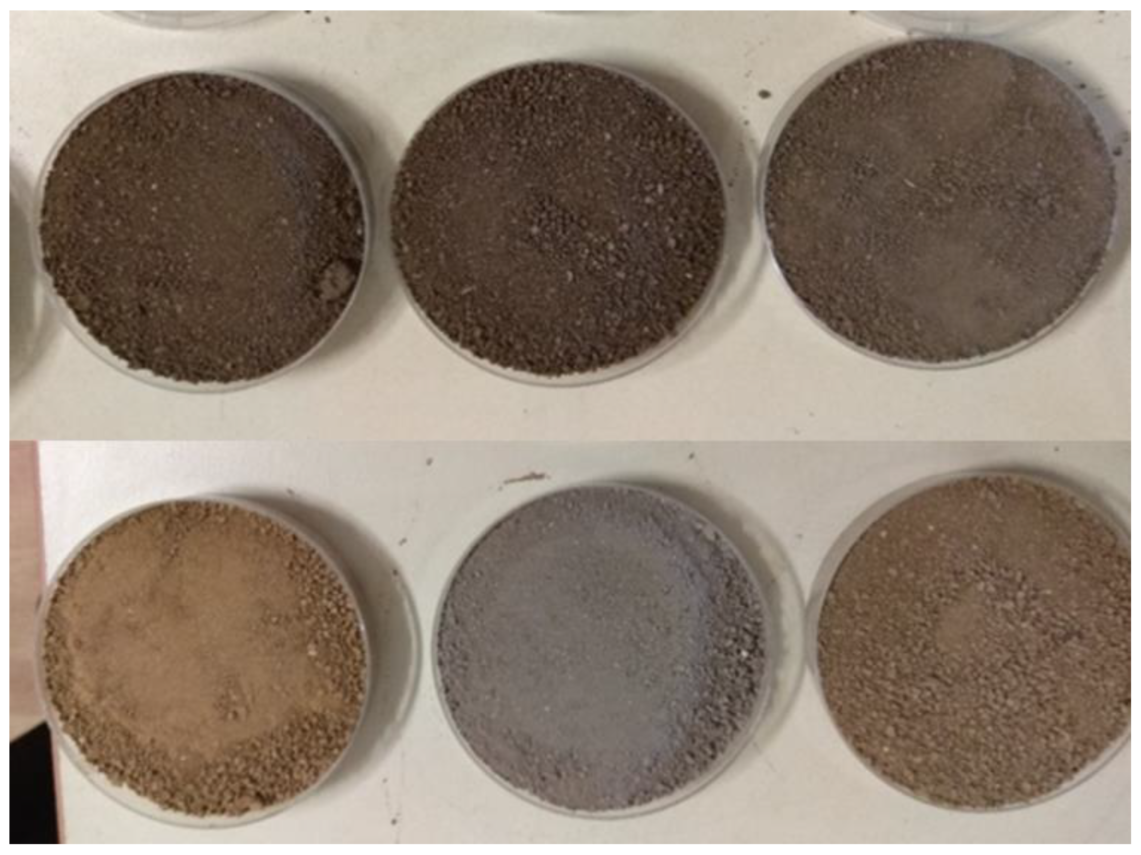
2.2. Soil Sampling and Chemical Analysis

Two extensive field campaigns took place to collect soil samples during September of 2018 and 2019. To select the sampling points, a random sampling design was performed prior to field visits to avoid systematic bias. For this, the sampling areas were preselected based on a bare/semi-bare soil mask based on Sentinel-2 imagery, and then, once in the field, this preselection was adjusted for some of the points to ensure that they were located in bare soil, as Sentinel-2 has some limitations in terms of the distinction of crops covered with residues and bare soil crops. Fifty-five (55) of these topsoil samples (0–10 cm) were utilized in this study. The respective soil samples were air-dried and large stones and plant residues were removed and then passed through a 2 mm sieve. The samples were separated into two subsamples and stored in sealed plastic bags for chemical analysis and spectral measurements. The SOM content was determined via the Walkley Black method i.e., soil C was estimated via a wet chemical method using potassium dichromate as an oxidizing agent [36], and the CaCO3 content was determined with the calcimeter method, where the calcium carbonate concentration is determined by the dissolution of carbonate in excess of 1N HCl [37]. The soil texture was also determined with the Bouyoucos method, where the size of the solids in the suspension was estimated from the density of the solution measured using the hydrometer [38].

2.3. Laboratory Spectral Measurements

The laboratory spectral measurements were performed in a controlled environment inside a dark box at the University of Thessaloniki. The instrument used was the PSR+ 3500, which has a spectral range of 350 to 2500 nm. The procedure was conducted in accordance with the protocol suggested by [39]. Initially, a white reference plate was measured for the calibration of the instrument, and then two distinct internal soil standards (ISS) were measured (Wylie Bay and Lucky Bay) The ISS were used to minimize systematic effects through the use of an agreed-upon and well-known material to align the readings of any method. In our case, two sand samples that maintain their properties over time were employed [39]. Lastly three measurements of each soil sample were taken and subsequently averaged. The same procedure was repeated in the same order after the measurement of five soil samples. Afterwards, the reflectance spectra were corrected using the ISS correction method.

2.4. HySpex Data Acquisition

The HySpex data were acquired during the EnMAP airborne Greece campaign, which was organized jointly by the GFZ Potsdam and the Free University Berlin and funded by the DLR/BMWi. The HySpex sensor consists of two separated push broom hyperspectral cameras, the HySpex VNIR-680 and the HySpex -SWIR 320m-e, which are manufactured by Norsk Elektro Optikk AS (NEO). The sensors have a spectral range of 400–2500 nm and a spectral sampling interval of 3.7 nm for VNIR (420–990 nm) and 6.0 nm for SWIR (970–2500 nm), resulting in a total of 408 spectral bands. The data were acquired on 16 September 2019 on a clear day, providing imagery with a spatial resolution of 1.9 m for the VNIR spectrometer and 4.0 for the SWIR-320m-e camera.
The hyperspectral images were radiometrically corrected and georectified, and the VNIR-SWIR was co-registered (for further details, see [40]). Physically based atmospheric correction of the HySpex data was carried out using sensor geometry for the separated VNIR and SWIR sensors with ATCOR-4 software [40], which is based on the atmospheric radiative transfer model MODTRAN 5. A rural aerosol model, a water vapor column of 1.0 g m−2, and a visibility of 120 km were selected as the atmospheric input parameters [41]. Finally, the single flight lines were mosaicked, providing imagery with a spatial resolution of 5 m in the finally processed georeferenced and stacked HySpex VNIR-SWIR mosaic data cube.
We excluded the spectral bands at 414–421 nm and 2413–2497 nm because of excessive noise. Additional bands (847–912 nm, 1321–1496 nm, and 1784–2025 nm) related to strong atmospheric absorptions were also removed from further analysis. Data were smoothed using a third-order Savitzky–Golay with a window size of 11 to make them more similar to the laboratory hyperspectral measurements.

2.5. PRISMA Data Acquisition

The Italian PRISMA (PRecursore IperSpettrale della Missione Applicativa) satellite, was launched in March 2019. It is equipped with a Hyperspectral Imager that uses a prism spectrometer and a panchromatic camera. The payload consists of the Hyp/Pan, optical heads, and the main electronics box units. A complete technical description is given in [42] including the pre- and in-flight radiometric calibration procedures as well as in [43,44]. The hyperspectral design is push-broom with 237 spectral bands at a spatial resolution of 30 m with a swath of 1000 pixels, while PAN provides images at a spatial resolution of 5 m (Table 1).
For the radiometric and geometric correction of the PRISMA L1B at-sensor radiance product, a processing chain originally developed for EO-1 Hyperion data [45,46] was adapted to provide PRISMA georeferenced surface reflectance imagery. Radiometric correction includes the removal of spectrally overlapping bands, bad band detection, and reductions for dead pixel and erroneous detector columns. An implementation of MODTRAN LUT based radiative transfer modeling proposed by [47] and originally designed for the EnMAP-Box [48] was used for the correction of atmospheric influence. It includes Aerosol Optical Thickness (AOT) and Columnar Water Vapor (CWV) retrieval as well as spectral Smile and adjacency correction [49]. For georeferencing, the original geographic LUT provided in the PRISMA L1B ancillary information was used to reproject the data by using the Bowtie Correction routine available in ENVI 5.56 software (L3Harris Technologies, Inc., Melbourne, FL, USA). Afterwards, a remaining geometric offset of 1–2 pixels (30–60 m) was further corrected by applying second-order polynomial rectification after the manual selection of in-scene Ground Control Points (GCPs) in QGIS3 (QGIS Association). The data acquisition occurred on 13 October 2019.

2.6. Data Preprocessing

Spectral data can be significantly influenced by effects like light scatter, which can be observed as baseline shifts or non-linearities [50]. In this study, several individual preprocessing methods and a combination of them were applied prior to the modeling procedure (Table 2). Specifically, the spectral data were converted from reflectance to absorbance data to highlight the absorption and potential underlying linear relationships between the absorption and properties. The first and second derivatives (1st and 2nd Savitzky–Golay derivatives) were used to determine the rate of change of the increase or decrease in absorption in order to normalize and differentiate the signal. The window size was adjusted to the spectral resolution of each sensor, as follows: laboratory, 101; HySpex, 29; and PRISMA, 11. The final preprocessing technique used was the normalization of the transformed data with the standard normal variate (SNV) to standardize the spectrum based on a mean value of 0 and a standard deviation of 1 in order to minimize the effects of scattering, noise, and extremes.

2.7. Predictive Algorithms

The multivariate data analysis was performed using the most common soil spectroscopy methods. These methods were the PLSR, Cubist, Random Forest, and Support Vector Machines. PLSR is used as the default method in the majority of the studies. Its usefulness is due to its ability to analyze data with many noisy, collinear, and even incomplete dependent and independent variables [51]. Unlike standard regression techniques (i.e., Ordinary Least Squares regression), PLSR is not affected by multicollinearity, which may occur when modeling a large number of independent variables and especially in datasets with a limited number of training instances. Furthermore, PLSR offers a reliable solution that combines dimensionality reduction through appropriate selection of the number of latent variables and the option to model multiple outcome variables. Cubist is an algorithm that was developed by Quinlan [52] and is used for the generation of rule-based models that produce accurate estimations by also maintaining a high degree of explainability. The Cubist algorithm combines the substantial parts of decision trees, rule-based approaches, and regression. Initially, a tree structure is created with every finite path deducted into a rule to define a subset. As a final step, regression is performed on each subset defined by the rules of the previous part of the algorithm. The tuning of Cubist algorithms enables the optimal selection of the number of neighbors and committees. Committees are sequential creations of iterative tree models, where the final prediction is the average of each model prediction. The Cubist algorithm uses a predefined set of nearest neighbors to adjust the rule-based model estimations by adjusting each prediction value according to the values of the training instances inside its neighborhood. This adjustment is weighted according to the inverse distance of each data point from the predicted value, so that proximal points contribute more to the adjustment. Random Forest (RF) regression is an ensemble learning algorithm that is widely used for the development of calibration models between diffuse reflectance measurements of soils and physicochemical analyses. It is classified as a supervised ensemble learning method that is based on a set of decision trees that are developed in parallel, and the output is the average of the estimations induced from each decision tree. The tuning of an RF model can be performed by assigning values to its three hyperparameters, the number of decision trees fitted, the number of variables over which each decision tree is developed, and the minimum node size, to control the size of each intermediate node and the size of the tree’s leaves. This parameter determines the nature of the algorithm, since the selection of a minimum node size of 1 will cause the algorithm to be a classifier, while larger values will enable the RF algorithm to perform a regression. In addition to the abovementioned techniques, the Support Vector Machines regressor was also evaluated for its capacity to produce accurate estimations of the SOM and CaCO3. The SVM is regarded as a nonparametric technique, since it does not rely on probability distributions but on kernel functions. The rationale for the functionality of this algorithm is to find a hyperplane that optimally separates the features into distinct groups. When features are not linearly separable, the Gaussian Kernel (or Radial basis function kernel), whose function is based on the feature distance from some initial point, can be employed. SVM tuning is performed by assigning values to the C and Gamma hyperparameters. C denotes the inverse of the strength of regularization and is thus the hyperparameter that defines the error tolerance of the algorithm, while Gamma defines the hyperplane’s curvature. In both cases, high values will result in model overfitting.
Model tuning was performed in each case through a grid search that extended to a wide range of hyperparameter values by exhaustively considering all parameter combinations. The values that induced minimized errors were selected as optimal.
The dataset used for the laboratory measurements was separated 30:70 into training and testing subsets, only considering information from spectral data captured from the PSR+ 3500. The split remained constant for each dataset and model iteration to enable a comparison between methods. For this purpose, the conditioned Latin Hypercube sampling (cLHS) algorithm was selected [53]. Each model was trained over the training dataset by employing the leave-one-out cross validation (LOOCV) method for hyperparameter tuning, while the overall performance of each trained model was evaluated through the testing subset.
For the HySpex and PRISMA spectral data, the LOOCV was utilized, as it was considered to be more appropriate for the small dataset [54]. The selection of the best-fitted model was performed through the quantification of model performance using typical error and variation-based metrics. The Root Mean Squared Error (RMSE), coefficient of determination (R2), and Ratio of Performance to InterQuartile distance (RPIQ) were calculated. These metrics were derived through a comparison between the observed (reference) and estimated property values (SOM and CaCO3) with the aim being to describe the relationships and the spread of residuals between these two sets of values. The analytical expressions of the abovementioned metrics are given below:
R M S E = i = 1 n ( y ^ i y i ) 2 n
R 2 = 1 i = 1 n ( y ^ i y i ) 2 i = 1 n ( y ¯ i y i ) 2
R P I Q = I Q y R M S E
where y ^ i denotes the estimated property values, y i represents the observed values, y ¯ i corresponds to the average observed value, and I Q y is the interquartile distance calculated from the observed values. The interpretation of the accuracy was in conducted in accordance with [55,56].
For the graphical representation of the modeling evaluation, a barplot with the values for each of the aforementioned metrics for the assessed model is provided. The best fitting model is represented by a scatterplot depicting the predicted against the observed values, including the 95% confidence interval. Data preparation, preprocessing, and analysis were performed with the R base package, while the modeling part was completed with the Caret package [57].

2.8. Datasets Used for Modeling

In this study, different datasets were used to perform the spectral modeling. The laboratory and HySpex datasets were the same. However, the PRISMA dataset was smaller because the acquired image did not cover the whole study area. The hyperspectral images (HySpex and PRISMA) were both taken in 2019. The HySpex image was acquired at the same time that soil sampling was performed, while the PRISMA image was acquired approximately four weeks later. Considering that SOM and CaCO3 do not show great changes within a year, we added samples from 2018 to the calibration/validation dataset. To select these samples, we applied a combination of two spectral indices and their respective thresholds in accordance with [58], i.e., a normalized difference vegetation index (NDVI) of <0.25 and a normalized Cellulose Absorption Index(nCAI) of <0.03, to identify bare soils in 2019. The outcome was a total of 55 soil samples to be utilized for the SOM estimation with the HySpex sensor and for the reference laboratory spectral measurements. As mentioned before, the PRISMA image did not cover the whole study area, and therefore, some of the soil samples were not included, resulting in a total of 30 samples being used. A laboratory chemical analysis of the CaCO3 content was only available for the 2019 field campaign, minimizing the size of the previous datasets. The datasets were defined as follows: 43 samples for the laboratory and HySpex calibration datasets and 25 samples for the PRISMA dataset (Table 3).

3. Results and Discussion

3.1. Soil Property Estimation

The results of the soil chemical analysis showed high variability in the SOM content, ranging from 0.9 to 8.6% (gravimetric percentage) with an average value of 3.5% and a standard deviation of 2.4. High SOM values were mainly located in the south, close to the mining area. The soils were shown to be rich in clay and showed a positive correlation with an increased SOM content. This was expected, as fine particles contribute to organic matter protection due to the formation of organo-mineral complexes that are resistant to microbial degradation [59]. The CaCO3 content also showed great variability, ranging from 0.5% to 62.3%, with an average value of 11.68% and a standard deviation of 18.52 (Table 4). This is attributed to the geological depositions of the region that belongs to the Pelagonian zone, where two separate carbonate covers were deposited on the margins east and west of this zone during the Triassic-Jurassic period [51]. Although the highest values were found to be located in the northern part of the study area, the majority of the samples had low values. The above findings are in accordance with the results of an independent study conducted by the prefecture of West Macedonia in the region.

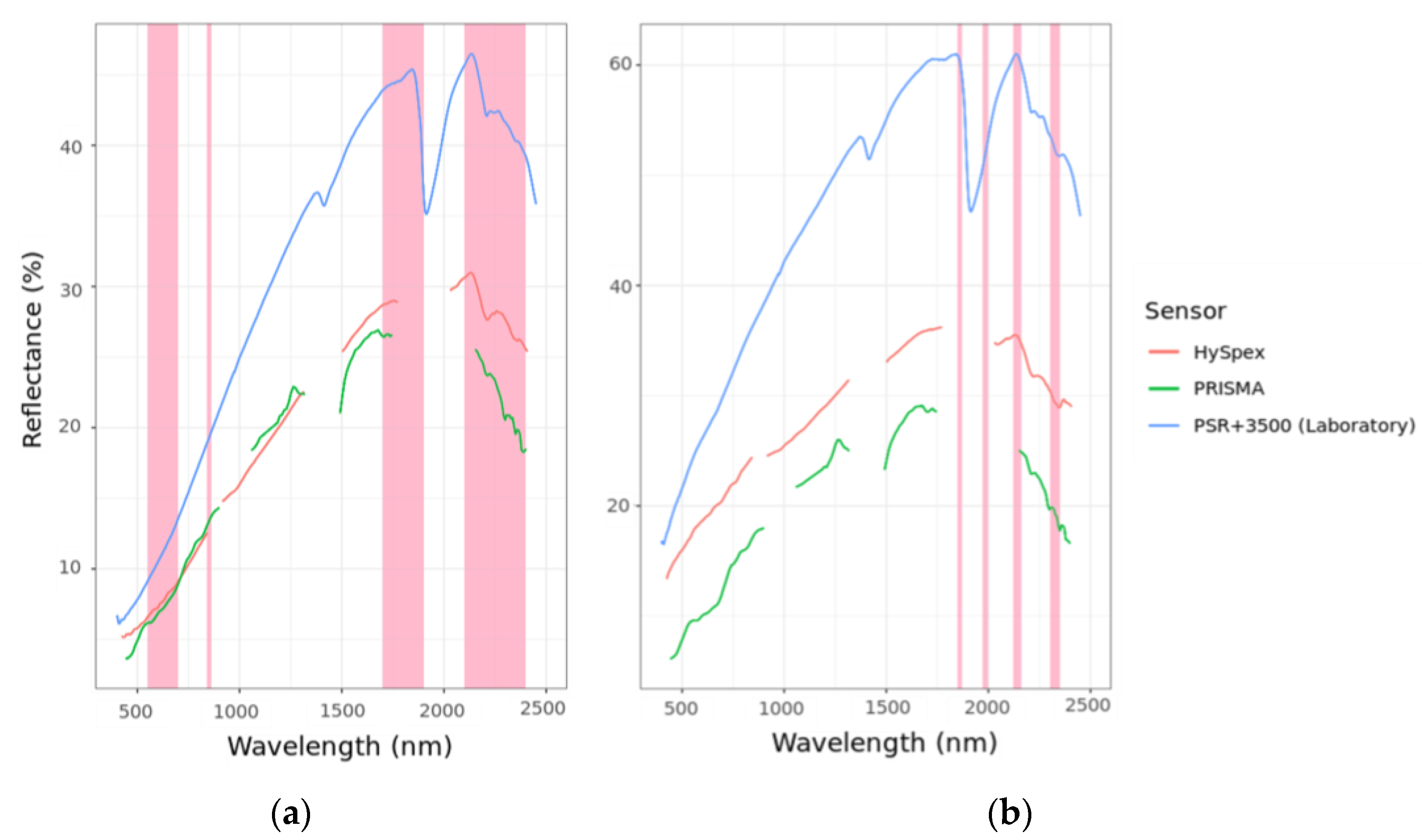
3.2. Spectral Data from the Three Different Sensors

The spectral signatures of the PSR+ 3500, HySpex, and PRISMA data are shown in Figure 3. Due to the controlled laboratory conditions used for the PSR+ 3500 measurements, reflectance was generally higher compared to that obtained with HySpex and PRISMA. This is due to differences in the field-of-view for acquisitions that are influenced by shading effects caused by rough terrain, like ploughing ridges. The reflectance intensity of soil samples with a high organic matter (OM) content was lower than the reflectance intensity of samples with a high CaCO3 content. This is to be expected, as soils rich in OM appear darker, while soils with a high carbonate content are usually lighter. This was also shown in the visible region by greater absorption in the shoulder of the spectral curve. The absorbance by carbonates can also be observed by the absorption peaks in the region, which were above 2100 nm [25] for all three sensors.

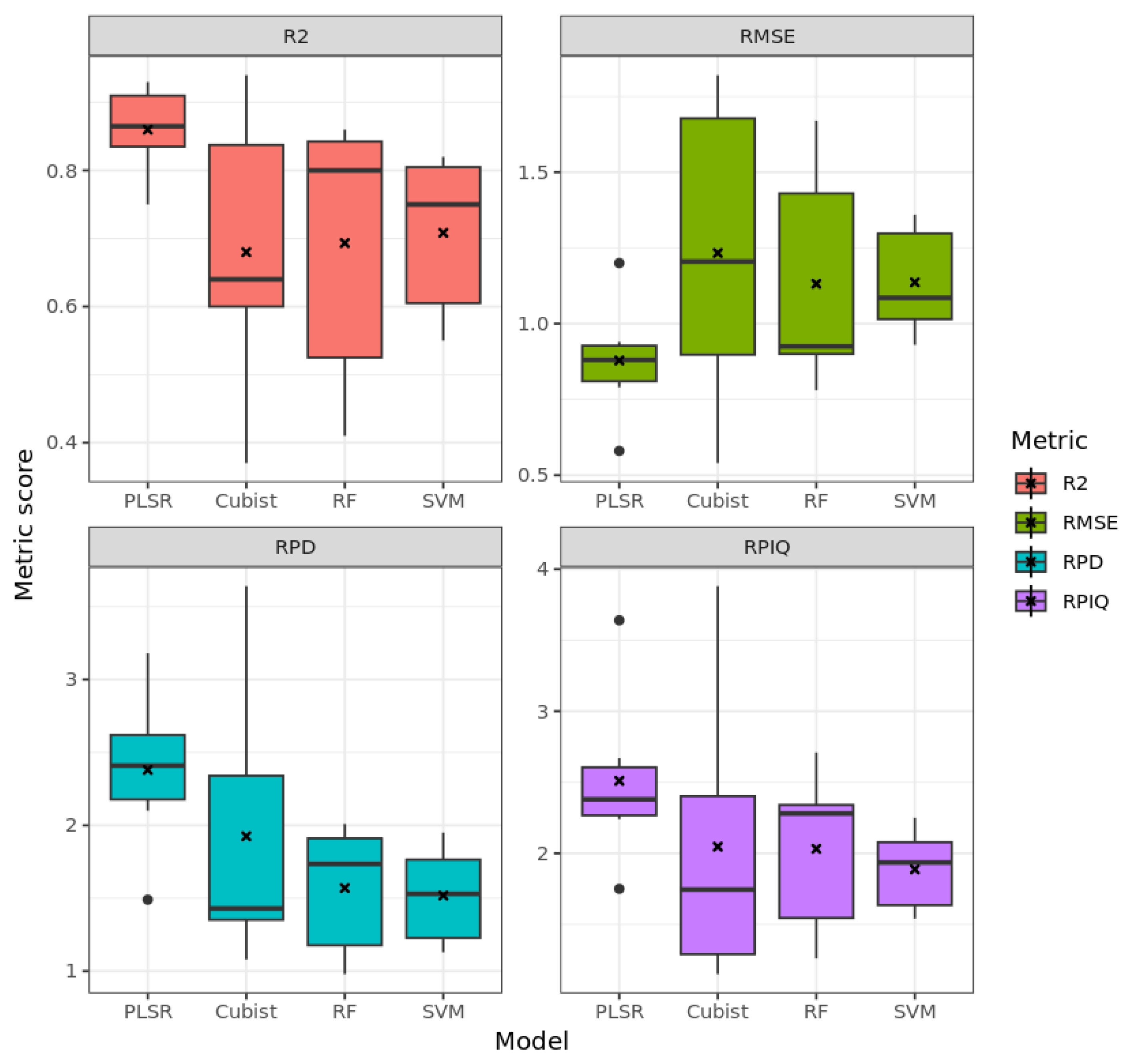
3.3. Model Performance for SOM

3.3.1. Laboratory Measurements

Four different modeling techniques, PLSR, Cubist, Random Forests (RF) and Support Vector Machines (SVM), were utilized (Figure 4). Laboratory spectral measurements showed great accuracy, with the Cubist algorithm and the combination of the log10(1/R) transformation, the 2nd Savitzky–Golay (w = 101), and a third-order polynomial coupled with Standard Normal Variate performing the best. Specifically, the RMSE was 0.54% and the R2 was 0.94 (Figure 5). The table with all the results can be found in Appendix A (Table A1).
In general, raw spectra showed the worst performance for all modeling algorithms. Studies have shown that using the 1st and 2nd derivatives improves the predictive performance of models [60] (Figure 6). The SNV results for the laboratory spectral measurements are consistent with those of previous studies as, in general, this method has a high accuracy. Specifically, for SOM/SOC estimations, R2 values of >0.81 have been reported [61,62,63,64]. PLSR had the highest R2 value, irrespective of the preprocessing method used, underlining why PLSR is so commonly used, especially for small datasets. However, the preprocessing method used did play an important role for other methods, particularly for the Cubist algorithm. Using the same combination of preprocessing methods as in this study, Ng et al. [65] reported a higher accuracy with PLSR than with the Cubist algorithm. In general, the use of a combination of preprocessing techniques improved the accuracy in most cases. When using the RF algorithm, it has been shown that the additional use of SNV does not improve the model’s accuracy and, in fact, reduces it. De Santana et al. [66] reported marginally better results when using RF compared with PLSR to predict the SOM content. The achievement of better results with the SVM algorithm compared with the PLSR were also reported by [67,68], while Stevens et al. [14] obtained a better performance with the Cubist algorithm over the SVM.

3.3.2. HySpex Data

The results based on the airborne HySpex imagery showed good accuracy, despite being lower than that of the laboratory measurements, which was expected due to the lower spectral resolution used (Figure 7). The best performing model (R2 = 0.79; RMSE = 1.07, RPD = 2.23) was the Cubist algorithm with preprocessing by absorbance transformation (log10(1/R)), the 1st derivative Savitzky–Golay (w = 29), and a 3rd-order polynomial (Figure 8). The use of the 1st derivative led to a better performance than the use of the 2nd derivative, irrespective of the use of SNV, expect for in the RF algorithm (Figure 9). The table with all the results can be found in Appendix A (Table A2).
These results are in accordance with those of other studies [32,69]. This may be attributed to the effects of the 1st and 2nd derivatives on the spectra. The 2nd derivative may reduce the quality of the spectra due to noise sensitivity and represents the curvature of the spectra, while the 1st derivative represents the slope of the spectra [70]. Looking at the results from all models, one can observe consistency in the accuracy level, with the exception of the SVM algorithm. In contrast to the results of our study, Xuemei et al. [68] reported that PLSR is not suitable for the estimation of the SOC from hyperspectral data. Stevens et al. [71] showed that the PLSR can perform marginally better than the SVM for regional calibrations with airborne hyperspectral data. The use of the SNV as an additional preprocessing method was shown to result in an improvement in the model accuracy, only for the RF algorithm.
Similar to the laboratory prediction models, the Cubist algorithm showed the best accuracy level. Regarding the preprocessing methods, the accuracy was affected by the order of the derivative. The Cubist algorithm produced more consistent results for the airborne, irrespective of the preprocessing methods used, while in the case of the laboratory measurements, the PLSR was most consistent.

3.3.3. PRISMA Data

The modeling results from the PRISMA spaceborne data showed a marginally reduced accuracy level compared to the airborne HySpex imagery (Figure 10). The best model performance (R2 = 0.76, RMSE = 1.22, RPD = 2.06, RPIQ = 3.31) was obtained with the Cubist algorithm with the following preprocessing methods: the 2nd derivative Savitzky–Golay (w = 11), 3rd-order polynomial, and SNV (Figure 11). The table with all the results can be found in Appendix A (Table A3).
Compared with the laboratory models, PRISMA data showed a greater accuracy with the addition of SNV preprocessing. This likely due to the usefulness of the SNV for correcting spectra for changes in the optical path length and light scattering. For the PRISMA data, there was no consistency regarding the accuracy and the order of the derivatives, and there were no high absorbance peaks, as indicated in the HySpex data (Figure 12). For the PLSR and SVM models, the accuracy dropped with an increase in the derivative order, while for the Cubist and RF algorithms, the opposite occurs. Τhese results are similar to those of Mzid et al. [72], who also reported a high level of accuracy for SOC estimations with the Cubist algorithm. Studies that utilized other satellite data (EO-1 Hyperion, Landsat ETM+, Sentinel-2) [16,73,74,75] have found lower accuracy levels than those obtained with PRISMA, which could be attributed to the lower spectral resolution used. PRISMA performs well for OM content estimations due to its high spectral resolution at the regions of the important wavelengths that indicate the presence of OM.

3.4. Model Performance for Carbonate Estimation (CaCO3)

3.4.1. Laboratory Data

All algorithms showed good results with the laboratory spectral measurements (Figure 13). The best performing models were the PLSR (R2 = 0.85, RMSE = 5.74) with preprocessing with absorbance (log10(1/R)), the 2nd derivative Savitzky–Golay (w = 101), and the SNV; and SVM (R2 = 0.8, RMSE = 5.22) without the SNV (Figure 14). The table with all the results can be found in Appendix A (Table A4).
The results are in accordance with a recent study by Asgari et al. [76], who also reported a high level of accuracy with the use of PLSR and SVM. Similar results were also reported by Conforti et al. [77], using PLSR. Overall, the models showed inconsistencies regarding the best preprocessing method, with the lowest accuracy generated with the Cubist algorithm. The use of the 2nd derivative gave better results in general, highlighting strong absorbance, except with the use of the Cubist algorithm (Figure 15). In comparison, Mammadov et al. [78], obtained more consistent results with this algorithm, irrespective of the preprocessing method. This could be attributed to the larger sample size needed for algorithms like Cubist. To improve the prediction accuracy, Qi et al. [79] developed a method to group spectral data according to their similarities. This method provided better results than grouping spectral data according to soil groups and could be useful for modeling data from different regions. Gomez et al. [80] showed that PLSR prediction models are not highly affected by the spatial extent of the study area, as CaCO3 predictions seem to fundamentally depend on the CO3 absorption bands that occur in the SWIR region.

3.4.2. HySpex Data

The CaCO3 estimation results showed large variability between models (Figure 16). The best predictive model (R2 = 0.82, RMSE = 7.85) from the HySpex data for the CaCO3 estimations was PLSR with no preprocessing (Figure 17). The table with all the results can be found in Appendix A (Table A5).
These results are comparable to those obtained in the study of Gomez et al. [30], who achieved a PLSR accuracy of R² = 0.77 for the carbonate content based on airborne HyMap data acquired in Southern France with similar preprocessing. The Cubist and RF algorithms showed moderate accuracy levels (R2 < 0.62), again without the use of preprocessing. In most cases, the use of the 1st derivative provided better results, i.e., for the PLRS 1st derivative, R2 = 0.5 and for the 2nd derivative, R2 = 0.39. However, in general, the models that underwent no preprocessing had higher accuracy levels. This could be attributed to the loss of the relatively sharp carbonate absorption feature in the SWIR region after the application of spectral smoothing (such as Savitzky–Golay filtering) (Figure 18). In general, PLS and machine learning approaches that exploit the full spectral range seem to provide more accurate retrieval of the carbonate content compared with feature-based spectral parametrizations, such as the Continuum Removal Absorption Depth (CRAD). This has been shown by Lagacherie et al. [31] on HyMap data (R2 = 0.61) and, recently, in a study by Mitran et al. [81], who used AVIRIS-NG airborne hyperspectral imagery for carbonate estimation based on a CRAD linear regression (R2 = 0.58).
Compared to laboratory predictive models, HySpex data showed better accuracy when the PLSR algorithm was used with no preprocessing. However, regarding the SVM algorithm, less accurate predictions were obtained compared to those obtained with laboratory data, which could be due to the lower data content.

3.4.3. PRISMA Data

PRISMA data showed lower accuracy levels compared to HySpex and laboratory data with significant differences between models (Figure 19). These differences were more evident compared to laboratory prediction models, which is explained by the large dissimilarities between the datasets. Similar to HySpex, the, best model (R2 = 0.36, RMSE = 11.25) had no preprocessing (Figure 20). The table with all the results can be found in Appendix A (Table A6).
In general, greater accuracy was attained with raw data, although this was still very low, and in this case, the use of the 1st derivative was better than the use of the 2nd derivative (Figure 21). These results are in accordance with those of Castaldi et al. [82] who also reported a low accuracy level when using Sentinel-2 and Landsat-8 data for CaCO3 predictions. These results can be attributed to the lack of exploitation of narrow spectral features in the SWIR region related to carbonates [83]. The poor results could also be attributed to the carbonate spectral range that shows distinctive absorption (>2100 nm). This is a region in which a low SNR could result in a loss of information for wavelengths of greater than 2300 nm. Another factor to consider is that the PRISMA image was acquired in the commissioning stage, and the final preprocessing procedure was not available at the time of data analysis. Other significant factors that can cause these inaccuracies for remote sensing applications are (i) the soil moisture; (ii) the soil roughness and mixed pixels with vegetation cover; and (iii) samples with low CaCO3 values that may be nondetectable from a spaceborne platform. In addition to this, PRISMA and HySpex images were acquired on different dates and thus are characterized by different environmental conditions (atmospheric, soil moisture, residual vegetation cover), which could have also caused differences in the accuracy level between the two sensors.

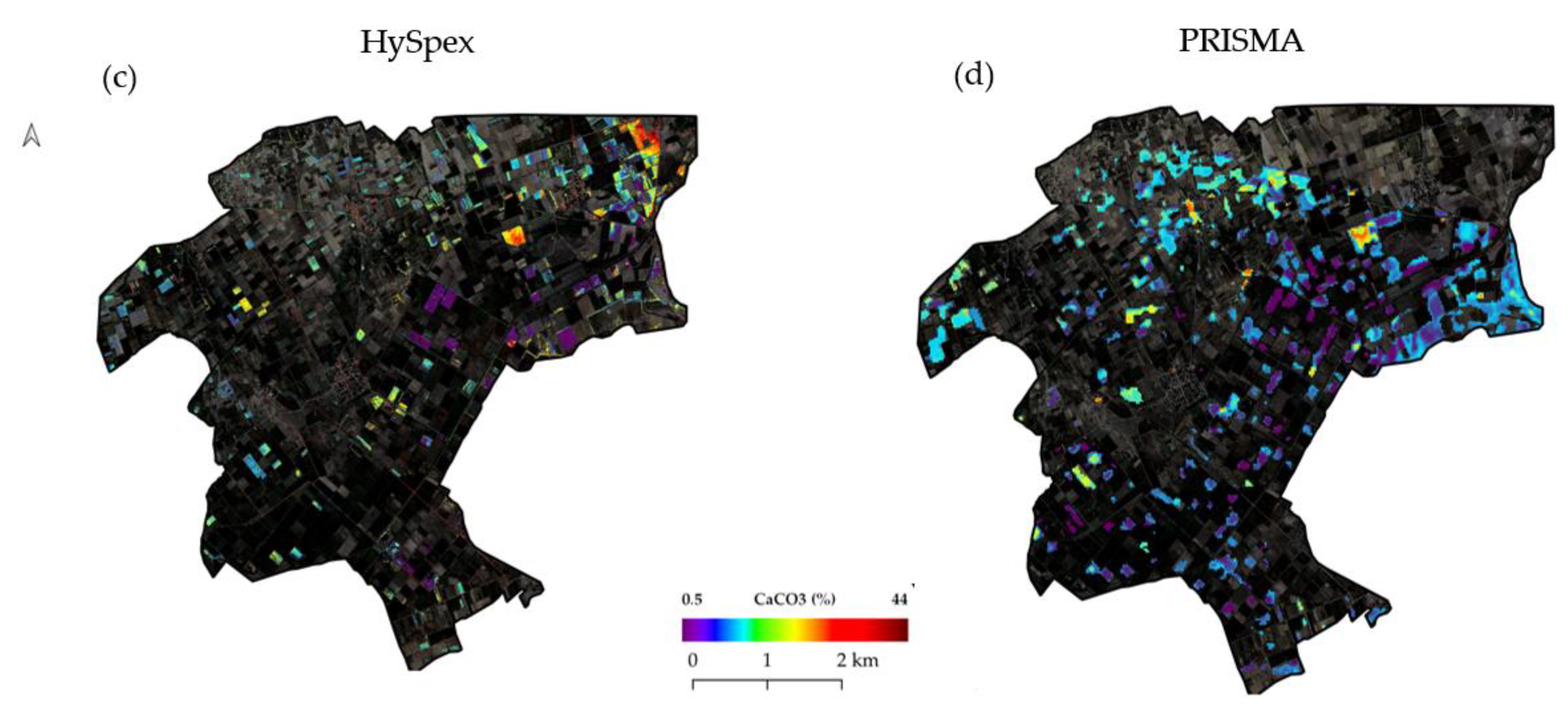
3.5. Spatial Distribution of Soil Properties

The spatial distribution of the soil properties was generated from the best models for each sensor and was applied to bare soil areas (Figure 22). Differences in the extent of the bare soil areas between the sensors are attributed to the different data acquisition dates. The PRISMA image was acquired one month later than the HySpex image, which resulted in more bare fields being present. In the northeast of the PRISMA acquisition area, no data were acquired due to reduced coverage. The OM prediction maps show similar spatial patterns of high and low concentrations, which are supported by the chemical analyses.
The best HySpex model was able to predict the mean concentrations of CaCO3 more accurately than the PRISMA model. However, areas with low CaCO3 contents were well predicted by both sensors. High values that were observed through chemical analyses in the northern study area were not well predicted by either sensor.

4. Conclusions

This study tested various preprocessing and calibration methods to estimate the SOM and CaCO3 contents on three different scales (laboratory, airborne, and spaceborne). The conclusions highlight the significance of selecting the proper preprocessing methods as well as the ideal calibration algorithm. As expected, the laboratory measurements showed a high level of accuracy, indicating the value of laboratory spectroscopy for estimating soil properties. The PLSR and Cubist algorithms were found to be the best models for predicting the SOM content. For the estimation of carbonates, all models showed good levels of accuracy; however, there was no particular consistency in terms of the preprocessing method. In most cases, however, the first derivative gave better prediction models than the second.
Both HySpex and PRISMA data were able to estimate the SOM content satisfactorily with comparable R2 and RPD values, and in some cases, the accuracy level was higher than previously reported in the literature using similar sensors. Slightly lower accuracy levels were obtained with PRISMA data, although this could be attributed to the lower SNR of the sensor, the spectral resolution, and the exclusion of significant bands during preprocessing. The results highlight the potential for the use of HySpex and PRISMA data for the estimation of SOM and CaCO3 contents from small datasets. Although carbonate prediction is still challenging at the spaceborne scale due to the low SNR in the SWIR, the modeling results at the laboratory and airborne scales mean that the estimation of the carbonate content with hyperspectral data can be considered feasible. Further research should focus on improving carbonate estimates using SWIR, preferably by employing larger and more diversified datasets. Our initial findings support the need for this further research, as the accuracy levels of PRISMA and HySpex signify possible underlying correlations that have not been fully exploited.
Model transferability from laboratory to airborne and spaceborne images is a concept that could highly benefit remote sensing applications, but further evaluation and more auxiliary properties are required to optimize the model’s performance.
The results of this study are very promising for future applications and the scientific use of PRISMA data for SOM estimation. Given that these were preliminary data obtained from the commissioning phase, one would expect that with the continued improvement of PRISMA products, they will become an invaluable asset in spaceborne hyperspectral imaging.

Author Contributions

Conceptualization, T.A., S.C. and G.Z.; methodology, T.A., R.M. and K.K.; software, T.A., R.M. and K.K.; validation, S.C., S.P. and G.Z.; formal analysis, T.A., R.M. and K.K.; investigation, T.A.; resources, S.C., S.P. and G.Z.; data curation, T.A., K.K., R.M., M.B. and T.R.; writing—original draft preparation, T.A., K.K. and R.M.; writing—review and editing, T.A., S.C., S.P., D.B. and G.Z.; visualization, T.A., K.K. and R.M.; supervision, T.A., S.C., S.P., D.B. and G.Z. All authors have read and agreed to the published version of the manuscript.

Funding

The authors acknowledge the EnMAP scientific preparation program (grant number 50EE1529) under the DLR Space Agency with resources from the German Federal Ministry for Economic Affairs and Climate actions for the funding of the 2019 Greece field and airborne campaign and associated research at the GFZ, co-funded by the Italian Space Agency (ASI) within the TEHRA project, Contract N. 2022-6-U.0, CUP F83C2200016000.

Acknowledgments

T.A. acknowledges an ERASMUS + grant for student traineeships at the GFZ-Potsdam. S.C., R.M. and M.B. thank the EnMAP science program funded by the German Federal Ministry for Economic Affairs and Climate actions and contributions through the DLR Space Agency. S.P. acknowledges co-funding from the Italian Space Agency (ASI) within the TEHRA project, Contract N. 2022-6-U.0, CUP F83C22000160005.

Conflicts of Interest

The authors declare no conflict of interest.

Appendix A

Table A1. Statistical evaluation of the models used to predict the soil organic matter (SOM) content from the laboratory data.
Laboratory (PSR+ 3500) (SOM)
PreprocessingModelRMSER2RPDRPIQ
1PLSR1.20.751.491.75
2PLSR0.890.832.12.35
3PLSR0.870.852.412.41
4PLSR0.940.882.412.24
5PLSR0.790.922.692.67
6PLSR0.580.933.183.64
1Cubist1.820.631.421.15
2Cubist1.820.371.081.16
3Cubist1.160.651.441.81
4Cubist0.540.943.643.88
5Cubist0.810.92.642.6
6Cubist1.250.591.331.68
1RF1.590.441.021.32
2RF1.670.410.981.26
3RF0.780.862.012.71
4RF0.90.851.942.34
5RF0.950.781.652.22
6RF0.90.821.822.34
1SVM1.360.561.131.54
2SVM1.360.551.181.55
3SVM1.060.761.791.98
4SVM1.110.741.371.89
5SVM0.930.821.952.25
6SVM10.821.692.11
Table A2. Statistical evaluation of the models used to predict the soil organic matter (SOM) content from the HySpex data.
HySPEX (SOM)
PreprocessingModelRMSER2RPDRPIQ
1PLSR1.430.661.682.77
2PLSR1.340.71.792.95
3PLSR1.340.71.792.95
4PLSR1.650.571.462.4
5PLSR1.260.721.913.15
6PLSR1.340.691.792.95
1Cubist1.480.611.622.67
2Cubist1.40.651.712.82
3Cubist1.070.792.233.69
4Cubist1.280.711.883.1
5Cubist1.160.762.073.42
6Cubist1.260.731.913.15
1RF1.670.511.442.38
2RF1.660.511.442.38
3RF1.360.691.772.92
4RF1.530.621.572.6
5RF1.40.671.722.83
6RF1.30.741.853.05
1SVM2.240.251.071.77
2SVM2.220.271.081.78
3SVM1.860.621.292.12
4SVM2.540.210.941.56
5SVM1.90.561.262.09
6SVM2.120.341.131.87
Table A3. Statistical evaluation of the models used to predict the soil organic matter (SOM) content from the PRISMA data.
PRISMA (OM)
PreprocessingModelRMSER2RPDRPIQ
1PLSR1.820.491.372.21
2PLSR1.760.531.432.3
3PLSR1.350.741.862.99
4PLSR1.520.631.652.65
5PLSR1.640.631.532.45
6PLSR1.980.41.272.04
1Cubist2.240.241.121.8
2Cubist1.560.61.612.58
3Cubist1.770.491.412.27
4Cubist1.40.721.792.88
5Cubist1.940.441.292.08
6Cubist1.220.762.063.31
1RF2.170.241.161.86
2RF2.170.231.151.85
3RF1.710.551.472.36
4RF1.660.621.512.42
5RF1.930.441.32.09
6RF1.90.481.322.13
1SVM2.50.161.011.61
2SVM2.530.10.991.59
3SVM1.970.511.272.04
4SVM2.50.271.011.61
5SVM2.010.471.252.00
6SVM2.090.441.21.93
Table A4. Statistical evaluation of the models used to predict the calcium carbonate content (CaCO3) from the laboratory data.
Laboratory (PSR+ 3500) (CaCO3)
PreprocessingModelRMSER2RPDRPIQ
1PLSR8.870.71.851.16
2PLSR5.740.852.551.79
3PLSR7.810.742.011.32
4PLSR9.60.711.81.07
5PLSR8.940.782.021.15
6PLSR4.660.852.531.88
1Cubist6.980.691.241.48
2Cubist7.770.742.011.33
3Cubist10.570.511.470.97
4Cubist10.730.341.130.96
5Cubist9.730.421.211.058
6Cubist14.930.030.480.59
1RF7.880.561.11.31
2RF7.760.571.131.33
3RF6.080.821.261.7
4RF8.330.661.181.24
5RF11.850.10.640.87
6RF8.080.60.741.09
1SVM7.290.621.261.41
2SVM6.750.71.241.53
3SVM7.060.661.621.46
4SVM5.220.861.731.97
5SVM7.370.621.221.4
6SVM6.240.81.411.41
Table A5. Statistical evaluation of the models used to predict the calcium carbonate content (CaCO3) from the HySpex data.
HySPEX (CaCO3)
PreprocessingModelRMSER2RPDRPIQ
1PLSR7.850.822.361.77
2PLSR13.120.541.411.06
3PLSR13.530.51.371.03
4PLSR16.380.391.130.85
5PLSR14.240.471.30.97
6PLSR14.130.521.310.98
1Cubist11.910.591.551.17
2Cubist11.580.61.61.2
3Cubist13.320.471.391.04
4Cubist17.050.231.080.81
5Cubist16.070.261.150.86
6Cubist19.450.030.950.71
1RF11.850.61.561.17
2RF11.730.621.581.18
3RF13.660.531.351.02
4RF16.920.161.090.82
5RF16.040.231.150.86
6RF16.050.251.150.86
1SVM17.830.391.040.78
2SVM17.930.381.360.77
3SVM19.50.460.950.71
4SVM19.860.170.930.7
5SVM18.080.131.020.77
6SVM18.690.020.990.74
Table A6. Statistical evaluation of the models used to predict the calcium carbonate content (CaCO3) from the PRISMA data.
PRISMA (CaCO3)
PreprocessingModelRMSER2RPDRPIQ
1PLSR11.250.361.240.2
2PLSR12.230.241.140.18
3PLSR13.30.161.050.17
4PLSR14.210.050.980.16
5PLSR13.780.141.010.16
6PLSR13.850.091.010.16
1Cubist12.540.271.110.18
2Cubist12.210.281.140.18
3Cubist16.260.040.860.14
4Cubist18.780.010.740.12
5Cubist13.430.151.040.17
6Cubist14.370.070.970.16
1RF13.820.041.010.16
2RF13.770.051.010.16
3RF12.820.151.090.17
4RF13.590.031.020.16
5RF13.10.091.060.17
6RF13.150.081.060.17
1SVM14.50.130.960.15
2SVM14.570.080.960.15
3SVM13.180.281.060.17
4SVM14.520.110.960.15
5SVM13.10.251.060.17
6SVM13.360.221.040.17

References

  1. FAO. Soil Organic Carbon the Hidden Potential; Food and Agriculture Organization: Rome, Italy, 2017; ISBN 9789251096819. [Google Scholar]
  2. Keesstra, S.D.; Bouma, J.; Wallinga, J.; Tittonell, P.; Smith, P.; Cerdà, A.; Montanarella, L.; Quinton, J.N.; Pachepsky, Y.; Van Der Putten, W.H.; et al. The significance of soils and soil science towards realization of the United Nations sustainable development goals. Soil 2016, 2, 111–128. [Google Scholar] [CrossRef] [Green Version]
  3. Osland, M.J.; Gabler, C.A.; Grace, J.B.; Day, R.H.; McCoy, M.L.; McLeod, J.L.; From, A.S.; Enwright, N.M.; Feher, L.C.; Stagg, C.L.; et al. Climate and plant controls on soil organic matter in coastal wetlands. Glob. Chang. Biol. 2018, 24, 5361–5379. [Google Scholar] [CrossRef]
  4. Scharlemann, J.P.; Tanner, E.V.; Hiederer, R.; Kapos, V. Global soil carbon: Understanding and managing the largest terrestrial carbon pool. Carbon Manag. 2014, 5, 81–91. [Google Scholar] [CrossRef]
  5. Wang, C.; Li, W.; Yang, Z.; Chen, Y.; Shao, W.; Ji, J. An invisible soil acidification: Critical role of soil carbonate and its impact on heavy metal bioavailability. Sci. Rep. 2015, 5, 12735. [Google Scholar] [CrossRef] [Green Version]
  6. Martin, J.B. Carbonate minerals in the global carbon cycle. Chem. Geol. 2017, 449, 58–72. [Google Scholar] [CrossRef]
  7. Goovaerts, P. Estimation or simulation of soil properties? An optimization problem with conflicting criteria. Geoderma 2000, 97, 165–186. [Google Scholar] [CrossRef]
  8. Ladoni, M.; Bahrami, H.A.; Alavipanah, S.K.; Norouzi, A.A. Estimating soil organic carbon from soil reflectance: A review. Precis. Agric. 2010, 11, 82–99. [Google Scholar] [CrossRef]
  9. Chabrillat, S.; Ben-Dor, E.; Rossel, R.A.V.; Demattê, J.A.M. Quantitative soil spectroscopy. Appl. Environ. Soil Sci. 2013, 2013, 1–3. [Google Scholar] [CrossRef] [Green Version]
  10. Stenberg, B.; Viscarra Rossel, R.A.; Mouazen, A.M.; Wetterlind, J. Visible and near infrared spectroscopy in soil science. Adv. Agron. 2010, 107, 163–215. [Google Scholar]
  11. Nocita, M.; Stevens, A.; van Wesemael, B.; Aitkenhead, M.; Bachmann, M.; Barthès, B.; Ben Dor, E.; Brown, D.J.; Clairotte, M.; Csorba, A.; et al. Soil Spectroscopy: An Alternative to Wet Chemistry for Soil Monitoring. Adv. Agron. 2015, 132, 139–159. [Google Scholar]
  12. Terra, F.S.; Demattê, J.A.M.; Viscarra Rossel, R.A. Spectral libraries for quantitative analyses of tropical Brazilian soils: Comparing vis-NIR and mid-IR reflectance data. Geoderma 2015, 255, 81–93. [Google Scholar] [CrossRef]
  13. Chabrillat, S.; Ben-Dor, E.; Cierniewski, J.; Gomez, C.; Schmid, T.; van Wesemael, B. Imaging Spectroscopy for Soil Mapping and Monitoring. Surv. Geophys. 2019, 40, 361–399. [Google Scholar] [CrossRef] [Green Version]
  14. Stevens, A.; Nocita, M.; Tóth, G.; Montanarella, L.; van Wesemael, B. Prediction of Soil Organic Carbon at the European Scale by Visible and Near InfraRed Reflectance Spectroscopy. PLoS ONE 2013, 8, e66409. [Google Scholar] [CrossRef]
  15. Rossel, R.A.V.; Behrens, T. Using data mining to model and interpret soil diffuse reflectance spectra. Geoderma 2010, 158, 46–54. [Google Scholar] [CrossRef]
  16. Castaldi, F.; Hueni, A.; Chabrillat, S.; Ward, K.; Buttafuoco, G.; Bomans, B.; Vreys, K.; Brell, M.; van Wesemael, B. Evaluating the capability of the Sentinel 2 data for soil organic carbon prediction in croplands. ISPRS J. Photogramm. Remote Sens. 2019, 147, 267–282. [Google Scholar] [CrossRef]
  17. Castaldi, F.; Chabrillat, S.; van Wesemael, B. Sampling Strategies for Soil Property Mapping Using Multispectral Sentinel-2 and Hyperspectral EnMAP Satellite Data. Remote Sens. 2019, 11, 309. [Google Scholar] [CrossRef] [Green Version]
  18. Angelopoulou, T.; Tziolas, N.; Balafoutis, A.; Zalidis, G.; Bochtis, D. Remote sensing techniques for soil organic carbon estimation: A review. Remote Sens. 2019, 11, 676. [Google Scholar] [CrossRef] [Green Version]
  19. Angelopoulou, T.; Balafoutis, A.; Zalidis, G.; Bochtis, D. From laboratory to proximal sensing spectroscopy for soil organic carbon estimation-A review. Sustainability 2020, 12, 443. [Google Scholar] [CrossRef] [Green Version]
  20. Ben-Dor, E.; Patkin, K.; Banin, A.; Karnieli, A. Mapping of several soil properties using DAIS-7915 hyperspectral scanner data—A case study over soils in Israel. Int. J. Remote Sens. 2002, 23, 1043–1062. [Google Scholar] [CrossRef]
  21. Vohland, M.; Ludwig, M.; Thiele-Bruhn, S.; Ludwig, B. Quantification of Soil Properties with Hyperspectral Data: Selecting Spectral Variables with Different Methods to Improve Accuracies and Analyze Prediction Mechanisms. Remote Sens. 2017, 9, 1103. [Google Scholar] [CrossRef] [Green Version]
  22. Steinberg, A.; Chabrillat, S.; Stevens, A.; Segl, K.; Foerster, S. Prediction of common surface soil properties based on Vis-NIR airborne and simulated EnMAP imaging spectroscopy data: Prediction accuracy and influence of spatial resolution. Remote Sens. 2016, 8, 613. [Google Scholar] [CrossRef] [Green Version]
  23. Castaldi, F.; Palombo, A.; Santini, F.; Pascucci, S.; Pignatti, S.; Casa, R. Evaluation of the potential of the current and forthcoming multispectral and hyperspectral imagers to estimate soil texture and organic carbon. Remote Sens. Environ. 2016, 179, 54–65. [Google Scholar] [CrossRef]
  24. Ward, K.J.; Chabrillat, S.; Brell, M.; Castaldi, F.; Spengler, D.; Foerster, S. Mapping Soil Organic Carbon for Airborne and Simulated EnMAP Imagery Using the LUCAS Soil Database and a Local PLSR. Remote Sens. 2020, 12, 3451. [Google Scholar] [CrossRef]
  25. Van Der Meer, F. Spectral reflectance of carbonate mineral mixtures and bidirectional reflectance theory: Quantitative analysis techniques for application in remote sensing. Remote Sens. Rev. 1995, 13, 67–94. [Google Scholar] [CrossRef]
  26. Ben-Dor, E.; Banin, A. Near-Infrared Reflectance Analysis of Carbonate Concentration in Soils. Appl. Spectrosc. 1990, 44, 1064–1069. [Google Scholar] [CrossRef]
  27. Summers, D.; Lewis, M.; Ostendorf, B.; Chittleborough, D. Visible near-infrared reflectance spectroscopy as a predictive indicator of soil properties. Ecol. Indic. 2011, 11, 123–131. [Google Scholar] [CrossRef]
  28. Ostovari, Y.; Ghorbani-Dashtaki, S.; Bahrami, H.-A.; Abbasi, M.; Dematte, J.A.M.; Arthur, E.; Panagos, P. Towards prediction of soil erodibility, SOM and CaCO3 using laboratory Vis-NIR spectra: A case study in a semi-arid region of Iran. Geoderma 2018, 314, 102–112. [Google Scholar] [CrossRef]
  29. Khayamim, F.; Wetterlind, J.; Khademi, H.; Robertson, A.H.J.; Cano, A.F.; Stenberg, B. Using visible and near infrared spectroscopy to estimate carbonates and gypsum in soils in arid and subhumid regions of Isfahan, Iran. J. Near Infrared Spectrosc. 2015, 23, 155–165. [Google Scholar] [CrossRef] [Green Version]
  30. Gomez, C.; Coulouma, G. Importance of the spatial extent for using soil properties estimated by laboratory VNIR/SWIR spectroscopy: Examples of the clay and calcium carbonate content. Geoderma 2018, 330, 244–253. [Google Scholar] [CrossRef]
  31. Lagacherie, P.; Baret, F.; Feret, J.B.; Madeira Netto, J.; Robbez-Masson, J.M. Estimation of soil clay and calcium carbonate using laboratory, field and airborne hyperspectral measurements. Remote Sens. Environ. 2008, 112, 825–835. [Google Scholar] [CrossRef]
  32. Gholizadeh, A.; Boruvka, L.; Saberioon, M.M.; Kozák, J.; Vašát, R.; Nemecek, K. Comparing different data preprocessing methods for monitoring soil heavy metals based on soil spectral features. Soil Water Res. 2015, 10, 218–227. [Google Scholar] [CrossRef] [Green Version]
  33. Viscarra Rossel, R.A.; Behrens, T.; Ben-Dor, E.; Brown, D.J.; Demattê, J.A.M.; Shepherd, K.D.; Shi, Z.; Stenberg, B.; Stevens, A.; Adamchuk, V.; et al. A global spectral library to characterize the world’s soil. Earth-Sci. Rev. 2016, 155, 198–230. [Google Scholar] [CrossRef] [Green Version]
  34. Samarinas, N.; Tziolas, N.; Zalidis, G. Improved Estimations of Nitrate and Sediment Concentrations Based on SWAT Simulations and Annual Updated Land Cover Products from a Deep Learning Classification Algorithm. ISPRS Int. J. Geo-Inf. 2020, 9, 576. [Google Scholar] [CrossRef]
  35. Tziolas, N.; Tsakiridis, N.; Ben-Dor, E.; Theocharis, J.; Zalidis, G. Employing a Multi-Input Deep Convolutional Neural Network to Derive Soil Clay Content from a Synergy of Multi-Temporal Optical and Radar Imagery Data. Remote Sens. 2020, 12, 1389. [Google Scholar] [CrossRef]
  36. Allison, L.E.; Black, C. Methods of soil analysis. Part 2. Chemical and microbiological properties. Agron. Monogr. 1965, 9, 1367–1378. [Google Scholar]
  37. Jackson, M.L. Soil chemical analysis-Advanced course, published by the author. Madison Wis. 1956, 991, 96. [Google Scholar]
  38. Bouyoucos, G.J. Hydrometer method improved for making particle size analyses of soils 1. Agron. J. 1962, 54, 464–465. [Google Scholar] [CrossRef]
  39. Ben Dor, E.; Ong, C.; Lau, I.C. Reflectance measurements of soils in the laboratory: Standards and protocols. Geoderma 2015, 245, 112–124. [Google Scholar] [CrossRef]
  40. Brell, M.; Rogass, C.; Segl, K.; Bookhagen, B.; Guanter, L. Improving Sensor Fusion: A Parametric Method for the Geometric Coalignment of Airborne Hyperspectral and Lidar Data. IEEE Trans. Geosci. Remote Sens. 2016, 54, 3460–3474. [Google Scholar] [CrossRef] [Green Version]
  41. Richter, R.; Schläpfer, D. Geo-atmospheric processing of airborne imaging spectrometry data. Part 2: Atmospheric/topographic correction. Int. J. Remote Sens. 2002, 23, 2631–2649. [Google Scholar] [CrossRef]
  42. Coppo, P.; Brandani, F.; Faraci, M.; Sarti, F.; Dami, M.; Chiarantini, L.; Ponticelli, B.; Giunti, L.; Fossati, E.; Cosi, M. Leonardo spaceborne infrared payloads for Earth observation: SLSTRs for Copernicus Sentinel 3 and PRISMA hyperspectral camera for PRISMA satellite. Appl. Opt. 2020, 59, 6888–6901. [Google Scholar] [CrossRef]
  43. Cogliati, S.; Sarti, F.; Chiarantini, L.; Cosi, M.; Lorusso, R.; Lopinto, E.; Miglietta, F.; Genesio, L.; Guanter, L.; Damm, A.; et al. The PRISMA imaging spectroscopy mission: Overview and first performance analysis. Remote Sens. Environ. 2021, 262, 112499. [Google Scholar] [CrossRef]
  44. Pignatti, S.; Amodeo, A.; Carfora, M.F.; Casa, R.; Mona, L.; Palombo, A.; Pascucci, S.; Rosoldi, M.; Santini, F.; Laneve, G. PRISMA L1 and L2 Performances within the PRISCAV Project: The Pignola Test Site in Southern Italy. Remote Sens. 2022, 14, 1985. [Google Scholar] [CrossRef]
  45. Rogass, C.; Guanter, L.; Mielke, C.; Scheffler, D.; Boesche, N.K.; Lubitz, C.; Brell, M.; Spengler, D.; Segl, K. An automated processing chain for the retrieval of georeferenced reflectance data from hyperspectral EO-1 HYPERION acquisitions. In Proceedings of the 34th EARSeL Symposium 2014, Warsaw, Poland, 16–20 June 2014; Volume 16, pp. 3.1–3.7. [Google Scholar]
  46. Milewski, R.; Chabrillat, S.; Behling, R. Analyses of Recent Sediment Surface Dynamic of a Namibian Kalahari Salt Pan Based on Multitemporal Landsat and Hyperspectral Hyperion Data. Remote Sens. 2017, 9, 170. [Google Scholar] [CrossRef] [Green Version]
  47. Guanter, L.; Richter, R.; Kaufmann, H. On the application of the MODTRAN4 atmospheric radiative transfer code to optical remote sensing. Int. J. Remote Sens. 2009, 30, 1407–1424. [Google Scholar] [CrossRef]
  48. Van der Linden, S.; Rabe, A.; Held, M.; Jakimow, B.; Leitão, P.J.; Okujeni, A.; Schwieder, M.; Suess, S.; Hostert, P. The EnMAP-Box—A Toolbox and Application Programming Interface for EnMAP Data Processing. Remote Sens. 2015, 7, 11249–11266. [Google Scholar] [CrossRef] [Green Version]
  49. Guanter, L.; Segl, K.; Sang, B.; Alonso, L.; Kaufmann, H.; Moreno, J. Scene-based spectral calibration assessment of high spectral resolution imaging spectrometers. Opt. Express 2009, 17, 11594–11606. [Google Scholar] [CrossRef] [Green Version]
  50. Rinnan, Å.; van den Berg, F.; Engelsen, S.B. Review of the most common pre-processing techniques for near-infrared spectra. TrAC Trends Anal. Chem. 2009, 28, 1201–1222. [Google Scholar] [CrossRef]
  51. Wold, S.; Sjöström, M.; Eriksson, L. PLS-regression: A basic tool of chemometrics. Chemom. Intell. Lab. Syst. 2001, 58, 109–130. [Google Scholar] [CrossRef]
  52. Breiman, L. Random Forests. Mach. Learn. 2001, 45, 5–32. [Google Scholar] [CrossRef] [Green Version]
  53. Minasny, B.; McBratney, A.B. A conditioned Latin hypercube method for sampling in the presence of ancillary information. Comput. Geosci. 2006, 32, 1378–1388. [Google Scholar] [CrossRef]
  54. Soriano-Disla, J.M.; Janik, L.J.; Viscarra Rossel, R.A.; Macdonald, L.M.; McLaughlin, M.J. The Performance of Visible, Near-, and Mid-Infrared Reflectance Spectroscopy for Prediction of Soil Physical, Chemical, and Biological Properties. Appl. Spectrosc. Rev. 2014, 49, 139–186. [Google Scholar] [CrossRef]
  55. Williams, P. Near-Infrared Technology: Getting the Best out of Light: A Short Course in the Practical Implementation of Near-Infrared Spectroscopy for the User; PDK Projects, Incorporated: Nanaimo, BC, Canada, 2004; ISBN 0975216708. [Google Scholar]
  56. Saeys, W.; Mouazen, A.M.; Ramon, H. AE—Automation and Emerging Technologies Potential for Onsite and Online Analysis of Pig Manure using Visible and Near Infrared Reflectance Spectroscopy. Biosyst. Eng. 2005, 91, 393–402. [Google Scholar] [CrossRef]
  57. Kuhn, M. Building predictive models in R using the caret package. J. Stat. Softw. 2008, 28, 1–26. [Google Scholar] [CrossRef] [Green Version]
  58. Chabrillat, S.; Guillaso, S.; Rabe, A.; Foerster, S.; Guanter, L. From HYSOMA to ENSOMAP—A New Open Source Tool for Quantitative Soil Properties Mapping Based on Hyperspectral Imagery from Airborne to Spaceborne Applications; EGU: Munich, Germany, 2016; Volume 18. [Google Scholar]
  59. Pietrzykowski, M.; Chodak, M. Near infrared spectroscopy—A tool for chemical properties and organic matter assessment of afforested mine soils. Ecol. Eng. 2014, 62, 115–122. [Google Scholar] [CrossRef]
  60. Guerrero, C.; Wetterlind, J.; Stenberg, B.; Mouazen, A.M.; Gabarrón-Galeote, M.A.; Ruiz-Sinoga, J.D.; Zornoza, R.; Viscarra Rossel, R.A. Do we really need large spectral libraries for local scale SOC assessment with NIR spectroscopy? Soil Tillage Res. 2016, 155, 501–509. [Google Scholar] [CrossRef]
  61. Jiang, Q.; Li, Q.; Wang, X.; Wu, Y.; Yang, X.; Liu, F. Estimation of soil organic carbon and total nitrogen in different soil layers using VNIR spectroscopy: Effects of spiking on model applicability. Geoderma 2017, 293, 54–63. [Google Scholar] [CrossRef]
  62. Sithole, N.J.; Ncama, K.; Magwaza, L.S. Robust Vis-NIRS models for rapid assessment of soil organic carbon and nitrogen in Feralsols Haplic soils from different tillage management practices. Comput. Electron. Agric. 2018, 153, 295–301. [Google Scholar] [CrossRef]
  63. Xu, S.; Zhao, Y.; Wang, M.; Shi, X. Comparison of multivariate methods for estimating selected soil properties from intact soil cores of paddy fields by Vis–NIR spectroscopy. Geoderma 2018, 310, 29–43. [Google Scholar] [CrossRef]
  64. Liu, Y.; Shi, Z.; Zhang, G.; Chen, Y.; Li, S.; Hong, Y.; Shi, T.; Wang, J.; Liu, Y.; Liu, Y.; et al. Application of Spectrally Derived Soil Type as Ancillary Data to Improve the Estimation of Soil Organic Carbon by Using the Chinese Soil Vis-NIR Spectral Library. Remote Sens. 2018, 10, 1747. [Google Scholar] [CrossRef] [Green Version]
  65. Ng, W.; Minasny, B.; Malone, B.; Filippi, P. In search of an optimum sampling algorithm for prediction of soil properties from infrared spectra. PeerJ 2018, 2018, e5722. [Google Scholar] [CrossRef] [PubMed] [Green Version]
  66. de Santana, F.B.; de Souza, A.M.; Poppi, R.J. Visible and near infrared spectroscopy coupled to random forest to quantify some soil quality parameters. Spectrochim. Acta Part A Mol. Biomol. Spectrosc. 2018, 191, 454–462. [Google Scholar] [CrossRef] [PubMed]
  67. Vohland, M.; Besold, J.; Hill, J.; Fründ, H.-C. Comparing different multivariate calibration methods for the determination of soil organic carbon pools with visible to near infrared spectroscopy. Geoderma 2011, 166, 198–205. [Google Scholar] [CrossRef]
  68. Xuemei, L.; Jianshe, L. Measurement of soil properties using visible and short wave-near infrared spectroscopy and multivariate calibration. Meas. J. Int. Meas. Confed. 2013, 46, 3808–3814. [Google Scholar] [CrossRef]
  69. Jiang, G.; Zhou, S.; Cui, S.; Chen, T.; Wang, J.; Chen, X.; Liao, S.; Zhou, K. Exploring the Potential of HySpex Hyperspectral Imagery for Extraction of Copper Content. Sensors 2020, 20, 6325. [Google Scholar] [CrossRef]
  70. Hong, Y.; Chen, Y.; Yu, L.; Liu, Y.; Liu, Y.; Zhang, Y.; Liu, Y.; Cheng, H. Combining fractional order derivative and spectral variable selection for organic matter estimation of homogeneous soil samples by VIS-NIR spectroscopy. Remote Sens. 2018, 10, 479. [Google Scholar] [CrossRef] [Green Version]
  71. Stevens, A.; Udelhoven, T.; Denis, A.; Tychon, B.; Lioy, R.; Hoffmann, L.; van Wesemael, B. Measuring soil organic carbon in croplands at regional scale using airborne imaging spectroscopy. Geoderma 2010, 158, 32–45. [Google Scholar] [CrossRef]
  72. Mzid, N.; Castaldi, F.; Tolomio, M.; Pascucci, S.; Casa, R.; Pignatti, S. Evaluation of Agricultural Bare Soil Properties Retrieval from Landsat 8, Sentinel-2 and PRISMA Satellite Data. Remote Sens. 2022, 14, 714. [Google Scholar] [CrossRef]
  73. Gomez, C.; Viscarra, R.A.; Mcbratney, A.B. Soil organic carbon prediction by hyperspectral remote sensing and fi eld vis-NIR spectroscopy: An Australian case study. Geoderma 2008, 146, 403–411. [Google Scholar] [CrossRef]
  74. Mirzaee, S.; Ghorbani-Dashtaki, S.; Mohammadi, J.; Asadi, H.; Asadzadeh, F. Spatial variability of soil organic matter using remote sensing data. Catena 2016, 145, 118–127. [Google Scholar] [CrossRef]
  75. Vaudour, E.; Gomez, C.; Fouad, Y.; Lagacherie, P. Sentinel-2 image capacities to predict common topsoil properties of temperate and Mediterranean agroecosystems. Remote Sens. Environ. 2019, 223, 21–33. [Google Scholar] [CrossRef]
  76. Asgari, N.; Ayoubi, S.; Demattê, J.A.M.; Dotto, A.C. Carbonates and organic matter in soils characterized by reflected energy from 350–25000 nm wavelength. J. Mt. Sci. 2020, 17, 1636–1651. [Google Scholar] [CrossRef]
  77. Massimo Conforti; Gabriele Buttafuoco Vis-NIR Spectroscopy for Determining Physical and Chemical Soil Properties: An Application to an Area of Southern Italy. Glob. J. Agric. Innov. Res. Dev. 2014, 1, 17–26. [CrossRef]
  78. Mammadov, E.; Denk, M.; Riedel, F.; Lewinska, K.; Kaźmierowski, C.; Glaesser, C. Visible and Near-Infrared Reflectance Spectroscopy for Assessment of Soil Properties in the Caucasus Mountains, Azerbaijan. Commun. Soil Sci. Plant Anal. 2020, 51, 2111–2136. [Google Scholar] [CrossRef]
  79. Qi, Y.; Qie, X.; Qin, Q.; Shukla, M.K. Prediction of soil calcium carbonate with soil visible-near-infrared reflection (Vis-NIR) spectral in Shaanxi province, China: Soil groups vs. spectral groups. Int. J. Remote Sens. 2020, 42, 2502–2516. [Google Scholar] [CrossRef]
  80. Gomez, C.; Lagacherie, P.; Coulouma, G. Continuum removal versus PLSR method for clay and calcium carbonate content estimation from laboratory and airborne hyperspectral measurements. Geoderma 2008, 148, 141–148. [Google Scholar] [CrossRef]
  81. Mitran, T.; Sreenivas, K.; Janakirama Suresh, K.G.; Sujatha, G.; Ravisankar, T. Spatial Prediction of Calcium Carbonate and Clay Content in Soils using Airborne Hyperspectral Data. J. Indian Soc. Remote Sens. 2021, 49, 2611–2622. [Google Scholar] [CrossRef]
  82. Castaldi, F. Sentinel-2 and landsat-8 multi-temporal series to estimate topsoil properties on croplands. Remote Sens. 2021, 13, 3345. [Google Scholar] [CrossRef]
  83. Gaffey, S. Spectral reflectance of carbonate minerals in the visible and near infrared (0.35–2.55 um). Anhydrous carbonate minerals. J. Geophys. Res. 1987, 92, 1429–1440. [Google Scholar] [CrossRef]
Figure 1. (right) Location of the study area and (left) true color HySpex imagery of the study area with the locations of the sampling points used for model calibration and validation.
Remotesensing 15 01106 g001
Figure 2. Different soil samples taken from the study area.
Remotesensing 15 01106 g002
Figure 3. Spectral signatures and important wavelengths in the PSR+ 3500, HySpex, and PRISMA data for high (a) OM and (b) CaCO3 values. The important spectral regions are highlighted in pink.
Remotesensing 15 01106 g003
Figure 4. Box plots of the accuracy metrics for the laboratory (PSR+ 3500) estimations of OM with the use of the PLSR, Cubist, RF and SVM algorithms for all preprocessing methods.
Remotesensing 15 01106 g004
Figure 5. Scatter plot of the best fitted model (Cubist, absorbance and Savitzky–Golay 2nd derivative) for OM prediction using the laboratory (PSR+ 3500) data, including the regression line (blue) with the 95% confidence interval (grey).
Remotesensing 15 01106 g005
Figure 6. 1st and 2nd derivatives of the laboratory (PSR+ 3500) spectral signature with a high OM content. The important spectral regions are highlighted in pink. The interval size varies according to the preprocessing method applied.
Remotesensing 15 01106 g006
Figure 7. Box plots for the accuracy metrics for HySpex estimations of OM with the use of the PLSR, Cubist, RF, and SVM algorithms for all preprocessing methods.
Remotesensing 15 01106 g007
Figure 8. Scatter plot of the best fitted model (Cubist, absorbance, and Savitzky–Golay 1st derivative) for the OM prediction using HySpex data, including the regression line (blue) with the 95% confidence interval (grey).
Remotesensing 15 01106 g008
Figure 9. 1st and 2nd derivatives of the HySpex spectral signature with a high OM content. The important spectral regions are highlighted in pink. The interval size varies according to the preprocessing method applied.
Remotesensing 15 01106 g009
Figure 10. Box plots for the accuracy metrics for PRISMA estimations of OM with the use of the PLSR, Cubist, RF and SVM algorithms for all preprocessing methods.
Remotesensing 15 01106 g010
Figure 11. Scatter plot of the best fitted model (Cubist, absorbance, Savitzky–Golay 1st derivative, and SNV normalization) for OM prediction using PRISMA data, including the regression line (blue) with the 95% confidence interval (grey).
Remotesensing 15 01106 g011
Figure 12. 1st and 2nd derivatives of a PRISMA spectral signature with a high OM content. The important spectral regions are highlighted in pink.
Remotesensing 15 01106 g012
Figure 13. Box plots for the accuracy metrics for the laboratory (PSR+ 3500) estimations of CaCO3 with the use of the PLSR, Cubist, RF and SVM algorithms for all preprocessing methods.
Remotesensing 15 01106 g013
Figure 14. Scatter plot of the best fitted model (PLSR, Absorbance, Savitzky–Golay 2nd derivative, and SNV normalization) for the CaCO3 predictions using the laboratory (PSR+ 3500) data, including the regression line (blue) with the 95% confidence interval (grey).
Remotesensing 15 01106 g014
Figure 15. 1st and 2nd derivatives of the laboratory (PSR+ 3500) spectral signature with a high CaCO3 content. The important spectral regions are highlighted in pink. The interval size varies according to the preprocessing method applied.
Remotesensing 15 01106 g015
Figure 16. Box plots for the accuracy metrics for HySpex estimations of CaCO3 with the use of the PLSR, Cubist, RF, and SVM algorithms for all preprocessing methods.
Remotesensing 15 01106 g016
Figure 17. Scatter plot of the best fitted model (PLSR, reflectance) for CaCO3 prediction using HySpex data, including the regression line (blue) with the 95% confidence interval (grey).
Remotesensing 15 01106 g017
Figure 18. 1st and 2nd derivatives of a HySpex spectral signature with a high CaCO3 content. The important spectral regions are highlighted in pink. The interval size varies according to the preprocessing method applied.
Remotesensing 15 01106 g018
Figure 19. Box plots for the accuracy metrics for PRISMA estimations of CaCO3 with the use of the PLSR, Cubist, RF and SVM algorithms for all preprocessing methods.
Remotesensing 15 01106 g019
Figure 20. Scatter plot of the best fitted model (PLSR, reflectance) for the CaCO3 prediction using PRISMA data, including the regression line (blue) with the 95% confidence interval (grey).
Remotesensing 15 01106 g020
Figure 21. 1st and 2nd derivatives of a PRISMA spectral signature with a high CaCO3 content. The important spectral regions are highlighted in pink. The interval size varies according to the preprocessing method applied.
Remotesensing 15 01106 g021
Figure 22. Prediction maps obtained from the best fitted models (a,b) for SOM, and (c,d) for CaCO3.
Remotesensing 15 01106 g022aRemotesensing 15 01106 g022b
Table 1. Main characteristics of PRISMA. The first column reports the MRD requirements, while the last three columns show the sensors’ performance levels, as derived by [43].
RequirementsVNIRSWIRPAN
Spectral range400–2500 nm400–1010 nm920–2500 nm400–700 nm
FWHM<15 nm9–13 nm9–14.5 nm-
Spectral bands 661711
SNR≥160–200 (400–450 nm)161–209 (400–450 nm)
≥200 (450–1000 nm)200–450 (450–1000 nm)
≥200 (1000–1750 nm)
≥100 (1950–2350 nm)
≥100 (PAN)
Swath width30 km; 2.77°
Ground Sampling Distance (GSD) 30 m30 m5 m
Table 2. Preprocessing methods applied to the spectral data (w = window size, p = polynomial order, the different window size numbers represent the different sensors (PSR+ 3500, HySpex and PRISMA respectively).
AbbreviationDescription of the Preprocessing Method
1no-preprocessing
2log10(1/R) reflectance to absorbance
3log10(1/R) and Savitzky–Golay 1st derivative, w = 101/29/11, p = 3
4log10(1/R) and Savitzky–Golay 2nd derivative, w = 101/29/11, p = 3
5log10(1/R) and Savitzky–Golay 1st derivative, w = 101/29/11, p = 3 and SNV
6log10(1/R) and Savitzky–Golay 2nd derivative, w = 101/29/11, p = 3 and SNV
Table 3. Number of samples used for model calibration/validation.
SensorSOMCaCO3
PSR+ 35005543
HySpex5543
PRISMA3025
Table 4. Descriptive statistics for SOM (Soil Organic Matter), CaCO3, and clay (N = 55).
SOM% (55)SOM% (30)CaCO3 (43) CaCO3 (25)Clay%
Min0.91.10.50.55
Max8.68.662.35059.9
Average3.53.811.687.530.39
Standard Deviation2.42.518.521419.02
Disclaimer/Publisher’s Note: The statements, opinions and data contained in all publications are solely those of the individual author(s) and contributor(s) and not of MDPI and/or the editor(s). MDPI and/or the editor(s) disclaim responsibility for any injury to people or property resulting from any ideas, methods, instructions or products referred to in the content.

