Greenhouse Gases Monitoring Instrument on GaoFen-5 Satellite-II: Optical Design and Evaluation

Abstract

The Greenhouse gases Monitoring Instrument on GaoFen-5 satellite-II (GMI-II) uses spatial heterodyne spectroscopy (SHS) for quantitative monitoring of atmospheric greenhouse gases (GHG). Unlike the traditional SHS, the interferometer component of the GMI-II was designed with zero optical path difference offset, effectively improving spectral resolution while maintaining the same detector specifications. The secondary imaging system with non-isometric scaling of spatial and spectral dimensions was designed to decrease the integration time of a frame image or improve the spectral signal-to-noise ratio (SNR) under the same integration time. This paper introduces the design, manufacture, adjustment methods, and test results of the main performance indexes of the GMI-II that indicate that the spectral resolution of the O₂ A-band detection channel is better than 0.6 cm⁻¹ and other channels are better than 0.27 cm⁻¹. Under the typical radiance of other carbon monitors’ on-orbit statistics, the spectral SNR of the GMI-II is more than 300. These test results demonstrate that the GMI-II can be well adapted to quantitative remote sensing monitoring of atmospheric GHG.

1. Introduction

Since the Industrial Revolution, the massive use of fossil fuels such as coal, oil and natural gas and the increase in human activities have altered the natural equilibrium composed of the atmosphere, ocean and biosphere, resulting in the increasing concentration of greenhouse gases (GHG) [1,2,3]. The latest Intergovernmental Panel on Climate Change (IPCC) report states that the global average temperature rise target is to be kept within 1.5 °C or 2 °C of pre-industrial by the end of the century [4]. According to the latest research results, if current emission levels are maintained, the temperature rise targets of 1.5 °C and 2 °C will be reached in 9.5 and 31 years, respectively [5]. Consequently, nations need to conduct more aggressive mitigation activities. Currently, the calculation of national GHG emissions is generally based on “down-up” statistical data such as activity level and emission factors, which has great uncertainty. Especially at the regional scale, the uncertainty is as high as 8–24%. In 2019, IPCC complemented the use of atmospheric concentration observations, particularly GHG fluxes of “up-down” inversion from satellite observations, to verify emissions inventories [6]. The primary detection means of GHG are ground-based observations and spaceborne observations. Ground-based observations are characterised by high detection accuracy and reliability but are subject to limited stations and lack global large-scale observation capability [7,8]. Spaceborne remote sensing technology with characteristics of large scale in space and continuous observation time can observe the North Pole and the South Pole, oceans, deserts, and other areas that are difficult for humans to reach. It is an essential means for the study of global changes in GHG [9].

Main atmospheric GHG, such as carbon dioxide, are permanent trace gases in the atmosphere. Due to atmospheric mixing, there is a tiny relatively concentration background in terms of concentration and concentration gradient. The research indicates that the atmospheric column-averaged CO₂ dry-air mixing ratio (XCO₂) at the regional scale of global observation is only as accurate as 1% (~4 ppm) or superior to decrease its uncertainty in climate research better [10]. It is difficult for GHG monitoring to enhance the detection accuracy of atmospheric CO₂ further and put higher demands on the instrument’s performance.

GHG spaceborne remote sensing detection technology can be divided into active and passive. On 16 April 2022, China launched the world’s first atmospheric environment monitoring satellite equipped with active lidar for CO₂ monitoring, aiming to achieve all-day, high-precision detection of atmospheric CO₂ [11]. Other CO₂ active detection payloads, such as ESA’s A-Scope and NASA’s ASCENDS, are planned [12,13,14]. The development of a combined active and passive payloads layout, with real-time calibration of passive observation through active observation data to compensate for shortcomings of ground-based observation sites, such as the insufficient number and differences in observation paths, may be one of the more promising directions for the future.

Passive remote sensing detection payloads applied in orbit are classified into Michelson interferometry, grating spectroscopy and Fabry-Perot Interferometric imaging spectroscopy (FPI). The OCO-2 (Orbiting Carbon Observatory-2) and OCO-3 launched by the United States in July 2014 and May 2019 [15,16,17], respectively, the ACGS (Atmospheric Carbon dioxide Grating Spectrometer) on China’s TanSat (Tan-Satellite) launched in December 2016 [18,19], and TROPOMI (TROPOspheric Monitoring Instrument) on board the ESA Sentinel-5 Precursor launched in October 2017 are all GHG detection payloads based on grating spectroscopy [20]. The GOSAT-FTS (Greenhouse gases Observing SATellite-Fourier Transform Spectrometer) on the GOSAT and the GOSAT2-FTS on the GOSAT2 launched by JAXA (Japan Aerospace Exploration Agency) in 2009 and 2019 [21,22], respectively, and the GAS (Greenhouse-gases Absorption Spectrometer) on the Chinese meteorological satellite FY-3D launched in 2017 [23] are all GHG detection payloads based on Michelson interferometric spectroscopy. Canada has launched six GHGSat payloads based on FPI in 2016, 2020, 2021 and 2022, respectively, and plans to launch a total constellation of 10 satellites by 2023 to monitor point-source emission fluxes at 25 m spatial resolution [24].

China launched GaoFen-5 Satellite-I (GF-5-I) and GF-5-II on 9 May 2018 and 7 September 2021 [25,26,27], respectively, carrying the Greenhouse gases Monitoring Instrument-I (GMI-I) and GMI-II, both developed by Anhui Institute of Optics and Precision Machinery, Chinese Academy of Sciences, which are based on spatial heterodyne spectroscopy (SHS) developed from Michelson interferometry. The GMI series of payloads are the first to apply SHS to the quantitative remote sensing monitoring of the absorption spectrum of GHG on board to obtain the global distribution of the concentration of CO₂ and CH₄, providing primary data for climate change research. GF-5-II carry six payloads, among which the DPC-II (Directional Polarization Camera-II) can detect optical and microphysical parameters of global atmospheric aerosols and clouds and provide effective data support for cloud discrimination and high-precision atmospheric radiation correction of the GMI-II.

In this paper, the interferometer assembly with Zero Optical Path Difference (ZOPD) offset and the secondary imaging system with non-isometric scaling in spatial and spectral dimensions are optimally designed according to the main technical specifications of the GMI-II. The assembly process has been optimised to enhance each detection channel’s spectral resolution and response under area array detectors with a limited number of pixels through the secondary matching of the interferometer zero frequency and spectral filter curves in the grating glueing process. The main performance indicators of the GMI-II have been tested. This paper provides a basis and reference for the on-orbit observation and data inversion of the GMI-II, thus ensuring that the CO₂ detection accuracy is better than 2~3 ppm. The GMI-II has completed testing and parameter optimisation on-orbit, and the data products have been produced monthly.

2. Detection Principle and Optimisation Design of the GMI-II

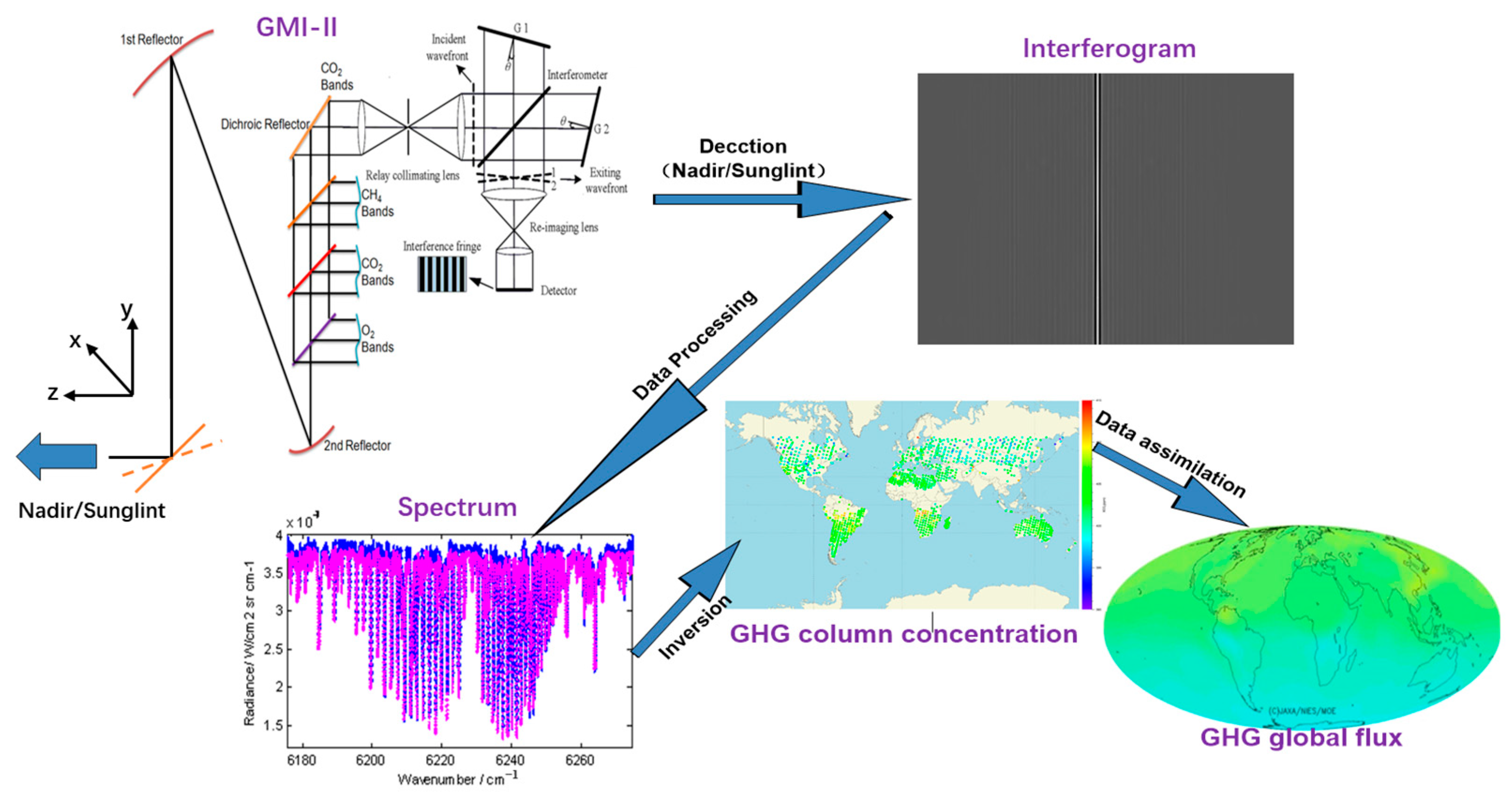
2.1. Detection Principle of the GMI

The GMI-II receives surface-reflected radiance, and the column concentration of GHG can be retrieved through the absorption spectrum. Similar to other carbon monitors, the GMI-II, designed with four spectral channels, selects visible and near-infrared (NIR) spectral regions as remote sensing spectral bands [28,29,30,31]. The selection basis and functions of each spectral channel are as follows.

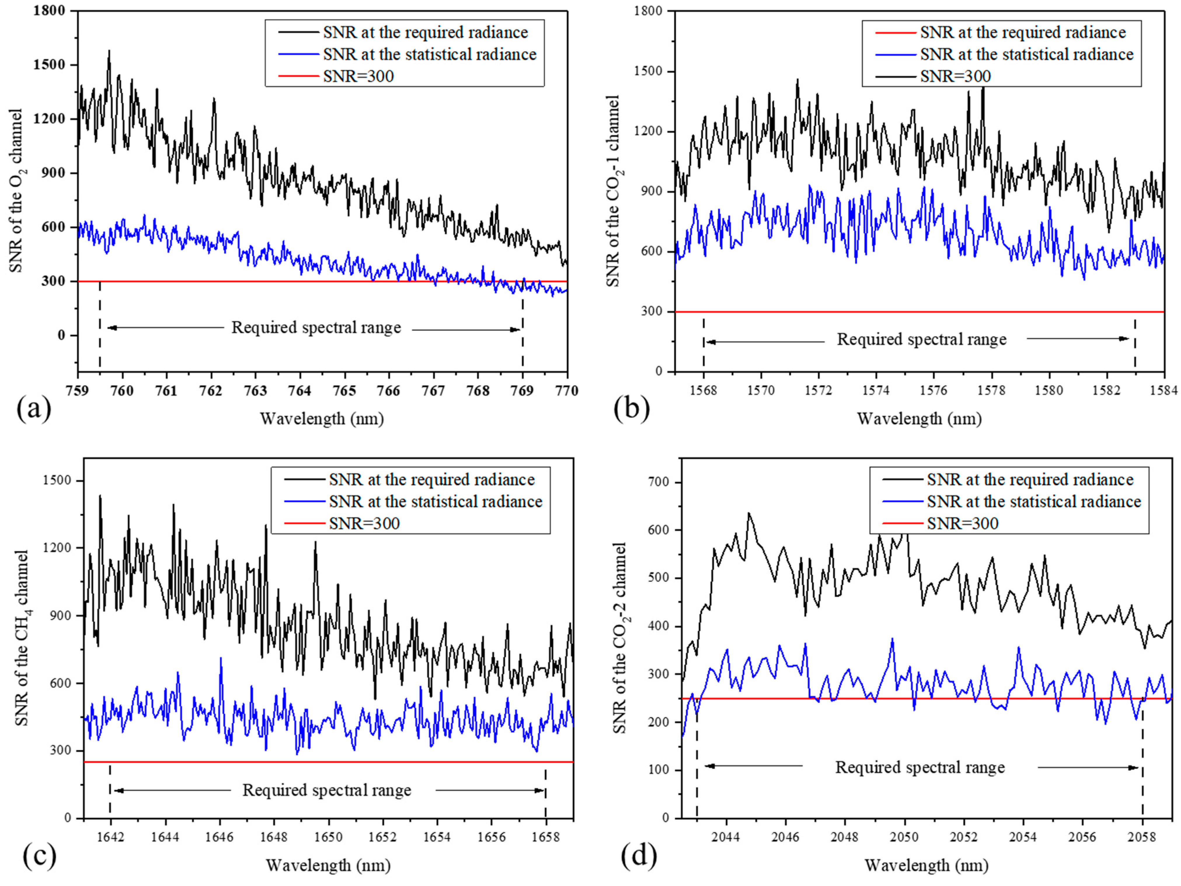
• Band 1: O₂ auxiliary observation channel (759–769 nm) is used to constrain the total atmospheric pressure of the surface, correct the systematic error of surface pressure, and also be used for cloud judgment and estimation of multiple scattering effects of aerosol under complex pollution conditions;
• Band 4: CO₂-1 channel (1568–1583 nm), the CO₂ weak absorption spectrum sensitive to concentration changes and fewer disturbing gases, used for inversion CO₂ column concentration in near-surface and troposphere;
• Band 3: CH₄ channel (1642–1658 nm), which is sensitive to CH₄ concentration changes and has fewer disturbing gases, is used to invert CH₄ column concentration;
• Band 2: CO₂-2 channel (2043–2058 nm), the CO₂ strong absorption spectrum, is weakly dependent on CO₂ concentration but sensitive to clouds and aerosols, synergistically correcting for the influence of ice clouds and aerosol scattering features on XCO2 and XCH4 in the NIR band during observations.

The detection principle of the GMI-II is illustrated in Figure 1. Firstly, the interferograms of four channels are directly obtained by the GMI-II, and the observed spectral curves are obtained by interference data processing. Then combines auxiliary parameters such as atmospheric conditions, surface characteristics and other information to produce GHG column concentration data products and carry out error analysis. Finally, the GMI-II produces GHG global flux data products after mapping and averaging [32].

The main specifications of the GMI-II are shown in

Table 1. Main specifications of the GMI-II.

Specifications	Values
	Band 1	Band 4	Band 3	Band 2
Detection gas	O2	CO2-1	CH4	CO2-2
Band range (nm)	759–769	1568–1583	1642–1658	2043–2058
Spectral resolution (cm−1)	0.6	0.27
SNR (albedo = 0.3; sun elevation = 30°)	300		250
Radiometric calibration	absolute accuracy: 5%; relative accuracy: 2%
FOV	14.6 mrad (10.3 km @ 705 km)
Scan	cross track: $\pm 35°$; along track: $\pm 20°$
Observation modes	nadir: 1, 5, 7, 9 points (default mode is 5 points); sun-glint

. The observation mode of the GMI-II is divided into the Nadir and Sun-glint modes. In the Nadir mode, the instantaneous spatial resolution is 10.3 km, and the width is realised by the rail-crossing point method of a two-dimensional tracking mirror. The four working modes are one point, five points, seven points, and nine points. The default working mode is five points, and the sampling point spacing is 100 km. In the Sun-glint mode, Sun-glint can be tracked autonomously according to solar azimuth, satellite attitude and other parameters. Nadir pointing accuracy and Sun-glint tracking accuracy of the two-dimensional tracking mirror are better than ± 0.1°.

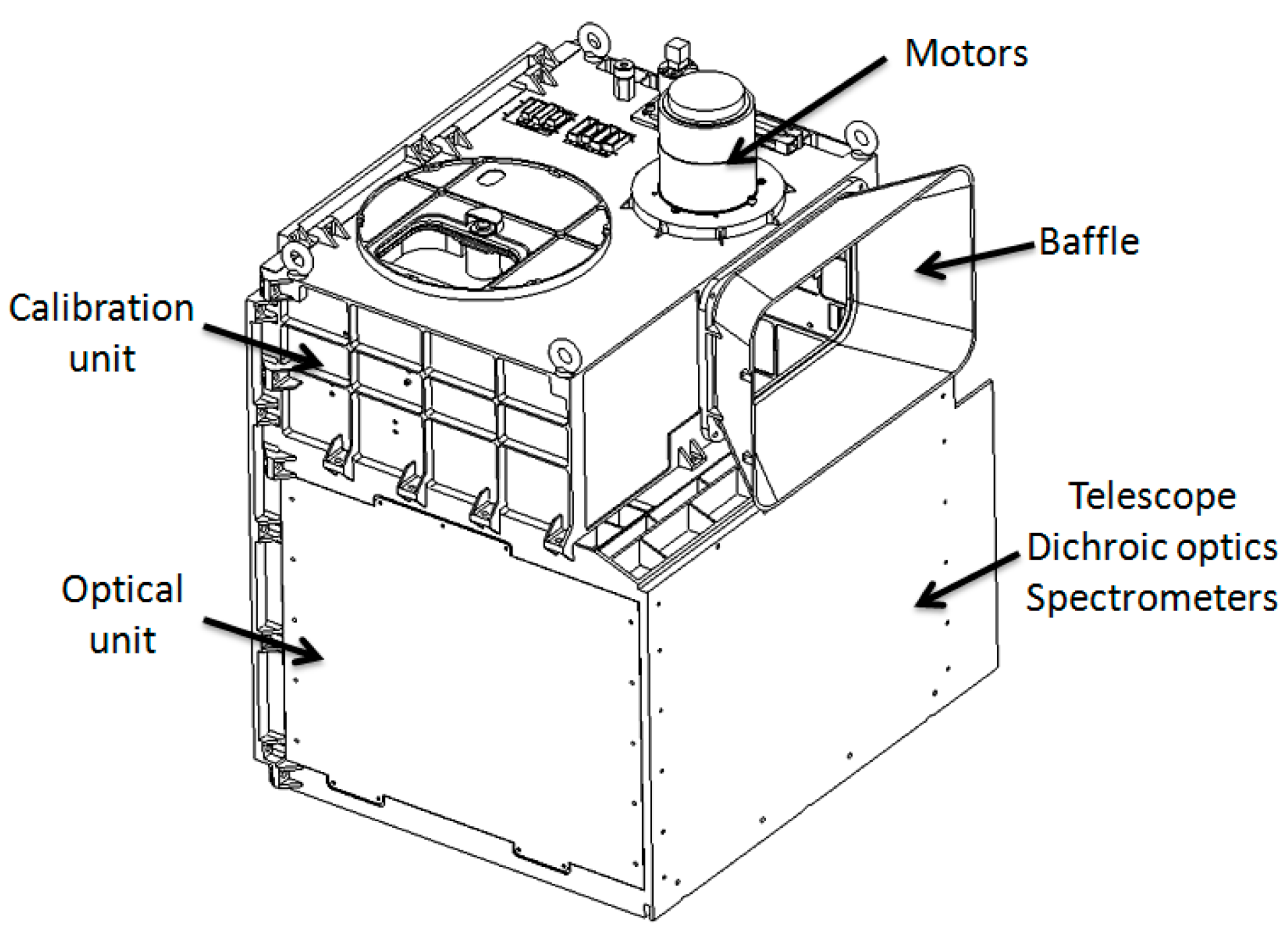
According to the function and performance requirements in Table 1, the GMI-II consists of the primary optics machine unit and calibration unit, as shown in Figure 2. The calibration unit mainly includes the 2D tracking mirror, calibration gate, light trap, diffuse reflector plate, and radiometer [33]. On the one hand, the 2D tracking mirror brings the sunlight into the instrument via a calibrated optical path to monitor changes in the instrument’s response in orbit. On the other hand, it enables wide-area spatial sampling by scanning along the track and cross-track. The primary optics machine unit is divided into five parts: telescope system, dichroic reflector module, collimation relay system, SHS, and secondary imaging system. The incident light is reflected by the 2D tracking mirror and enters the Gregory reflector telescope. Then the beam diameter is compressed and enters the dichroic reflectors. It is divided into four bands, and the SHS modulates the incident light of each band. The secondary imaging system images the interferogram to a CCD detector (759~769 nm band), a HgCdTe (MCT) detector (2043~2058 nm band), and two InGaAs detectors (1568~1583 nm, 1642~1658 nm band).

2.2. Optical Design of Telescope System and Collimation Relay System

According to the performance of the application requirements (spatial resolution, spectral resolution, spectral range, SNR, and others), specifications and performance of the selected detector (pixel size, pixel number, sensitivity, spectral response, and others) and constraints on resources provided by the satellite platform (volume, weight), the optical system scheme and design parameters (aperture, field of view (FOV) angle, spectral response) of the GMI-II are determined by a comprehensive engineering trade-off.

The primary optical system of the GMI-II is divided into five parts, whose functions are as follows.

• The telescope system, composed of the Gregorian off-axis telescoping system, gathers radiation information of surface reflection and atmospheric scattering of the spatial resolution element. The FOV angle of the telescope system, which is 14.6 mrad, is determined by the 708.45 km orbit altitude of the satellite, observation mode and corresponding spatial resolution of 10.5 km. The telescope system compresses the optical path with an aperture of 14.6 mrad small FOV and 105 mm large diameter in the clear aperture to reduce the size and weight of subsequent optical paths.
• The dichroic reflector component pre-distinguishes the effective spectral range of the four channels.
• The collimation relay system collimates the parallel light from the telescope system for a second time to meet the effective clear aperture, FOV and interference wavefront of the interferometer assembly and positions the exit pupil on the grating surface to maximise the illumination uniformity and energy utilisation of the interferogram.
• The SHS assembly, composed of ten optical components including a beamsplitter, spacers, field-widened prisms and gratings, combines spatial interference and grating diffraction to modulate light of different wavelengths into interference fringes of different spatial frequencies at the interference localisation plane.
• The secondary imaging system requires a specific scaling ratio in the grating dispersion direction, i.e., the image size of the interferometric localisation plane (determined by the spectral resolution and grating groove density) to be scaled in a fixed proportion to the focal plane and requires the energy to be focused on the focal plane as much as possible in the grating groove direction [34].

The design of the optical system starts from the interferometer assembly, takes the SNR requirement as the premise, and combines the grating groove density that can be obtained and manufactured, spectral resolution, optional detector parameters, and other information to determine the incident FOV and clear aperture of the interferometer assembly for each channel. Then the incident pupil diameter and the zoom ratio of the telescope system are computed, and the second imaging system is designed for each channel.

In the nadir observation mode, the SNR of the instrument is mainly related to the detector performance and optical system design parameters. The SNR is calculated as follows [35].

$$SNR=\frac{S}{{\epsilon }_{eff}}=\frac{S}{\sqrt{{\epsilon }_D^2+{\epsilon }_R^2+S}},$$

(1)

where, ${\epsilon }_D$ is a dark scattering noise, a random noise generated by the detector’s dark current, independent of the signal level and related to the integration time and detector’s operating temperature; ${\epsilon }_R$ is a readout noise generated during the generation of an electronic signal, independent of both the signal level and detector’s operating temperature, and caused by the detector’s drive design; $S$ the number of photons on each pixel. In addition to the above factors, the SNR of SHS in the spectral domain is also related to the interferometric modulation efficiency, which is generally considered 0.75 or more for monochromatic light [36].

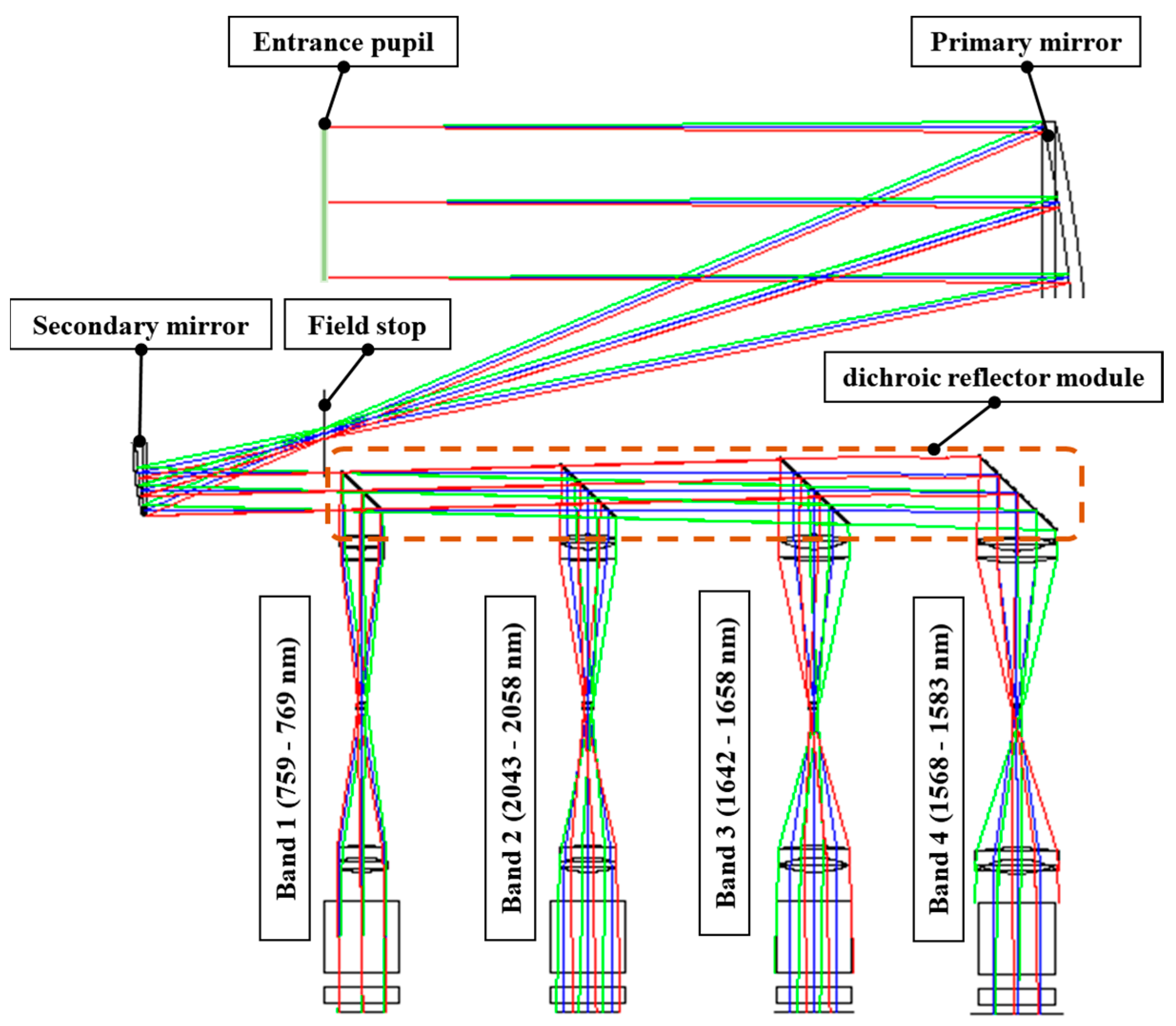
Based on the SNR review and the engineering experience of the preliminary principle prototype development, the interferometer components were pre-designed. Then the detailed design of the front telescope system, four-channel colour separation components and corresponding collimation system optical path were completed, and the front optical path layout is illustrated in Figure 3. Due to the wide detection band (757 nm to 2043 nm) and small FOV (14.6 mrad), a reflective system was considered, with a Gregorian off-axis telescope system consisting of parabolic and ellipsoidal mirrors without central blocking. The light beam is reflected by each channel’s corresponding dichroic reflector component into the corresponding collimation relay system to avoid achromatic aberrations. At the same time, considering that there are only two surfaces in the reflective optical system, we have used aspherical surfaces to control aberrations. In the design of the telescope system, in order to reduce the machining difficulty of the 2D tracking mirror and consider the necessary space required for the installation and movement of the 2D tracking mirror, we selected the 2D tracking mirror as the instrument entrance pupil to design the front function component of the optical system.

According to the above requirements, the results of the design of the front telescope system are as follows.

• The telescopic system with a scaling ratio of 5:1 and an exit pupil diameter of 21 mm;
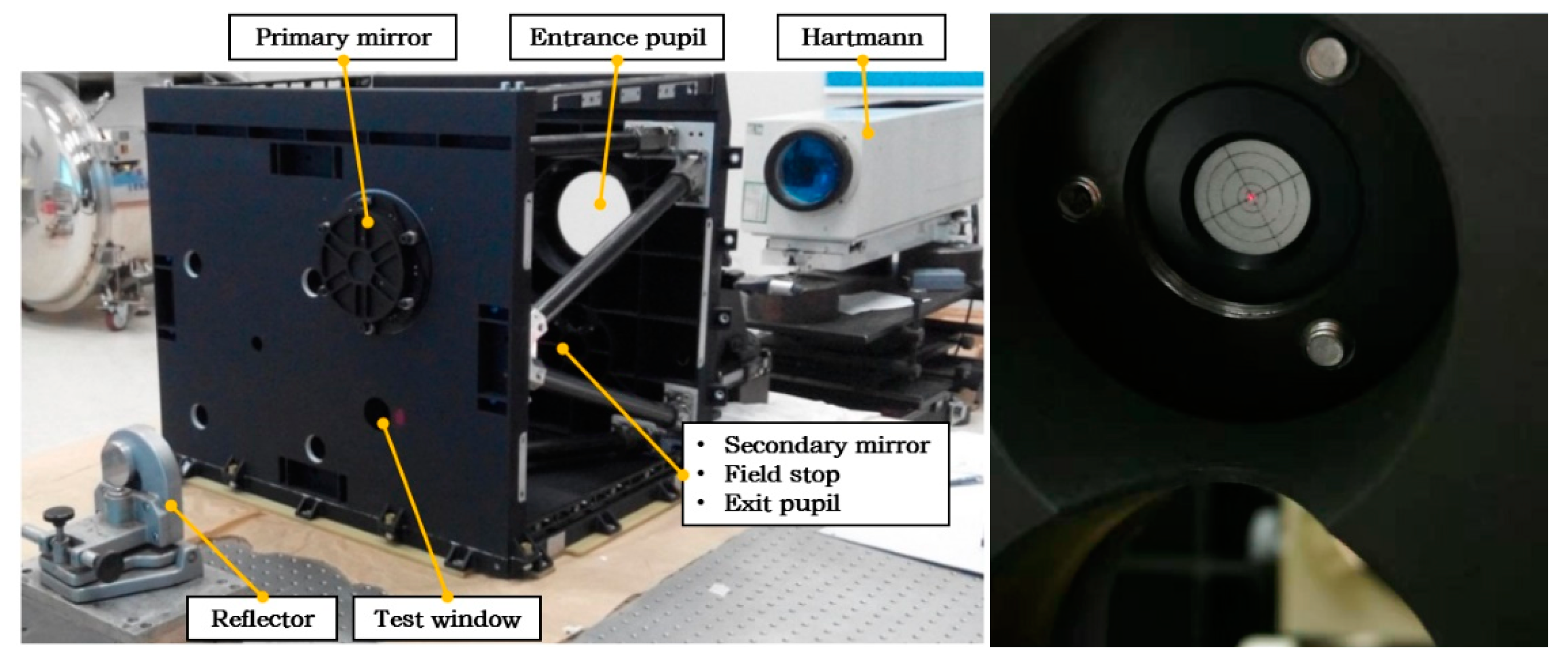
• The spacing between the primary and secondary mirrors is 198 mm, and the off-axis dimensions of the primary and secondary mirrors are 165 mm and 33 mm, respectively, to provide effectively installed space for the field stop, aperture for eliminating stray light and four-channel spectrometers;
• The field stop is located at the real image plane of the primary mirror, and the FOV of the four channels are unified through the field stop;
• A polariser is installed at the telescope system’s exit pupil to decrease the residual polarisation sensitivity of the GMI-II;
• The interferometric localisation planes of the four channels are the conjugate plane of the exit pupil of the telescope system to ensure uniformity of illumination at the interference fringe;
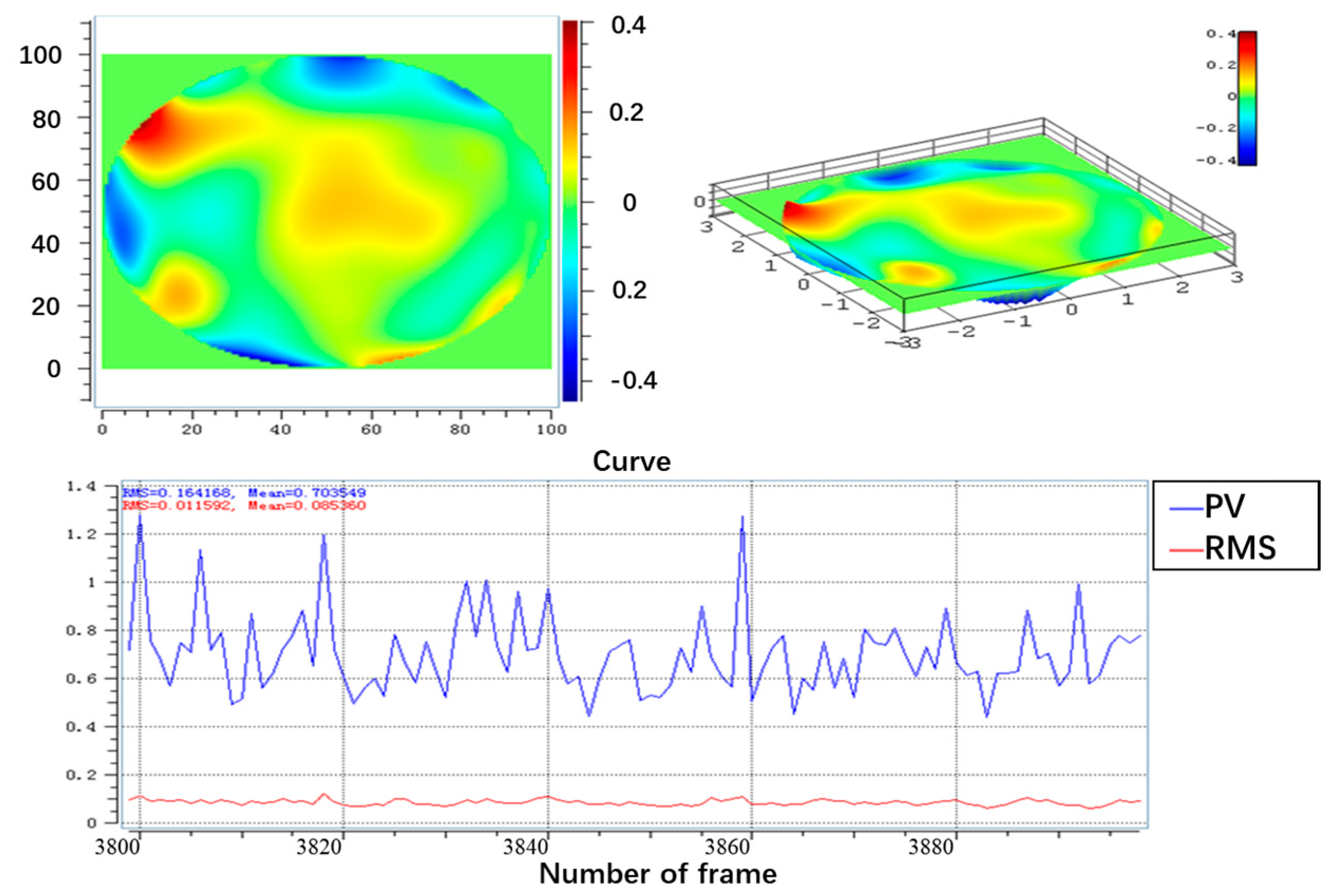
• The root means square (RMS) of the exiting wavefront is better than 1/4 wavelength for each channel.

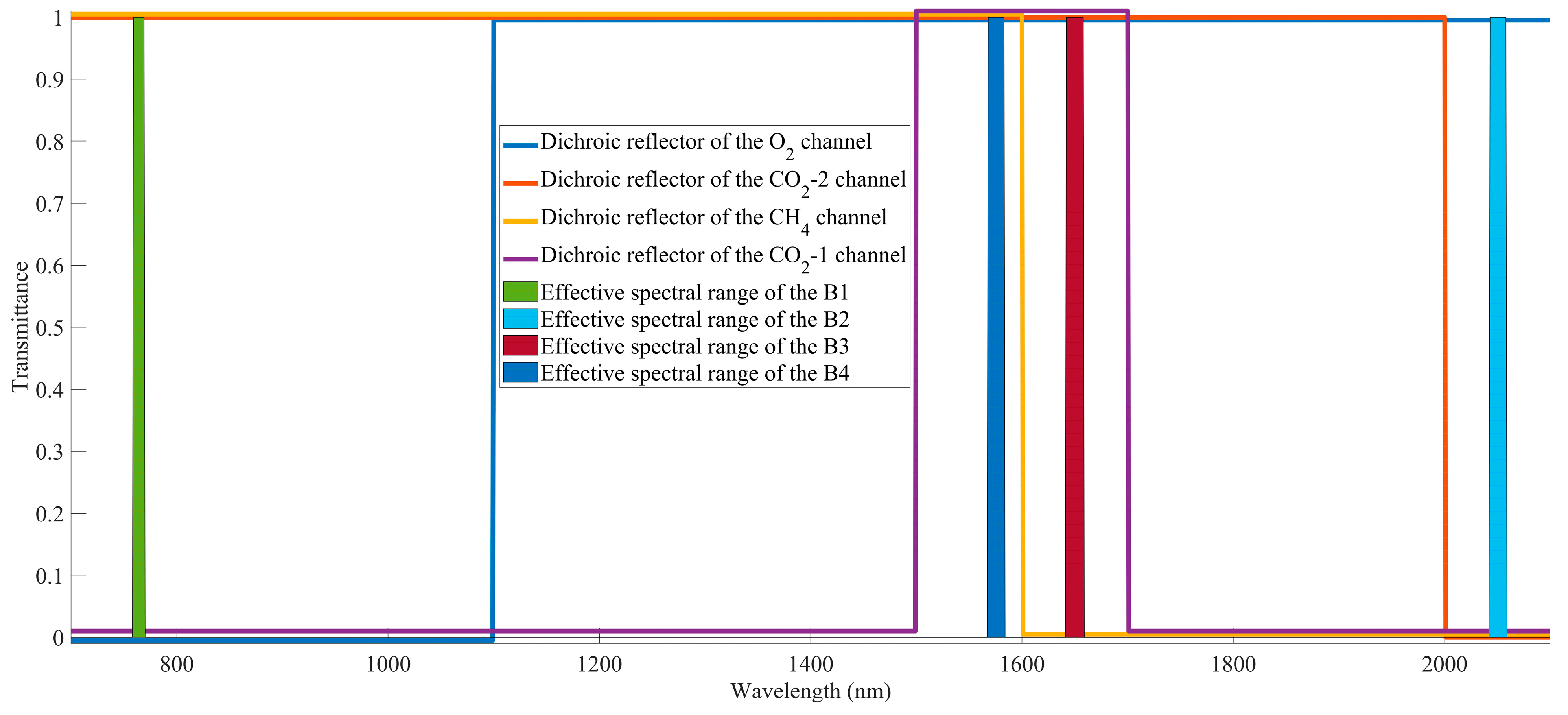
Figure 4 illustrates the distribution of spectral curves of the dichroic reflectors of four channels based on the reflection system’s spectral range (700~2100 nm). The GMI-II does not simply follow a wavelength sequence in its optical layout. First, the light below 1100 nm is reflected by the O₂ channel; then, the 1550–1680 nm light is transmitted by the dichroic reflector of the CO₂-2 channel. The channel layout is to reduce the pressure of the dichroic reflectors of the two adjacent spectral channels, CO₂-1 and CH₄, and to ensure the optical system efficiency of the short-wave infrared (SWIR) CO₂-2 channel as much as possible.

The spacing of the dichroic reflectors determines the installation space of the spectrometers of each channel. It is necessary to consider the compact design of lens components, the driving circuit size of focal plane components and the installation structure of the thermal control module.

2.3. Optical Design of Asymmetric Interferometers

The interferometer assembly is the core module for the main technical specifications, such as spectral range, resolution, and luminous flux, and is the primary starting point for the optical design of the GMI-II. According to the technical index requirements described in Table 1, the pixel number of available detectors for the three main observation channels cannot simultaneously meet spectral resolution and range requirements. Consequently, the interferometer design with ZOPD offset is carried out for the three main observation channels to solve the difficulties of high spectral resolution, spectral range and sampling ratio to satisfy the technical index requirements simultaneously under the restricted detector pixel number [37].

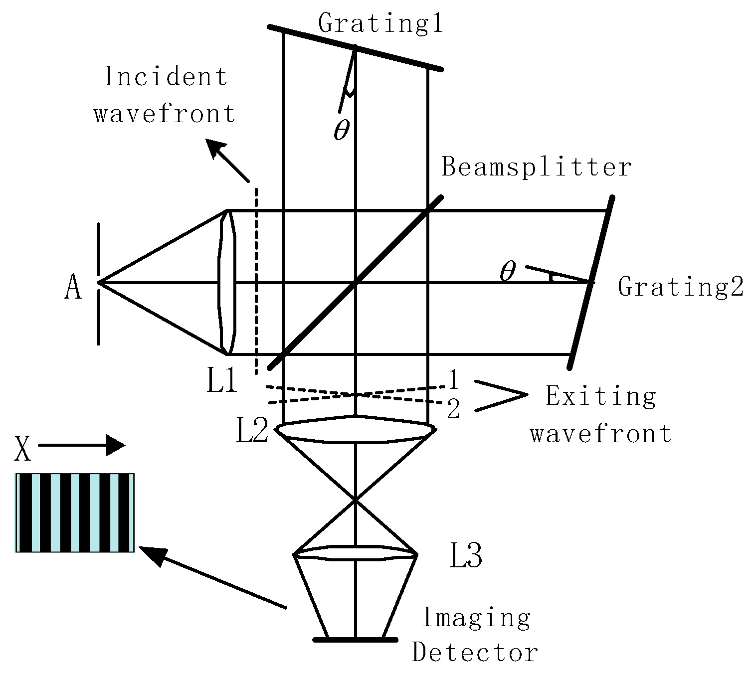
The principle of traditional SHS is illustrated in Figure 5. The collimating lens transforms the light source or target with a specific FOV into a parallel beam incident to the beamsplitter and then becomes two coherent beams with approximately equal energy. The beams are diffracted by gratings in two arms and are returned to the beamsplitter. Interference fringes are formed on the grating surface, i.e., the localisation surface, finally scaled by the secondary imaging system and received by the detector. A reference wavelength is selected to effectively form measurable low-frequency spatial interference fringes, giving a very high spectral resolution in narrow spectra.

The interferometer essentially follows the principle of two-beam interference. Considering only monochromatic light σ in the dispersion direction, the interference intensity $I\left(x,f_{\sigma }\right)$ produced by the wave vectors of two arms can be expressed as:

$$I\left(x,f_{\sigma }\right)=I_1+I_2+2\sqrt{I_1{I}_2}cos(2\pi x{f}_{\sigma }),$$

(2)

$$f_{\sigma }=4\left(\sigma -{\sigma }_0\right)tan{\theta }_L,$$

(3)

where, $I_1, I_2$ are the radiation intensity of the two beams; x denotes the coordinates of the dispersion direction relative to the ZOPD position; $f_{\sigma }$ represents the spatial frequency of interference fringe corresponding to wavenumber $\sigma$; ${\sigma }_0$ and ${\theta }_L$ are the reference wavenumber and Littrow angle, respectively, and the interference frequency of the incident light satisfying these two parameters is 0.

When the two arms are equal in length along the optical axis direction, as shown in Figure 5, the optical axis (i.e., x = 0) is located at the ZOPD position, and the expression of optical path difference (OPD) U and the coordinate x of relative ZOPD in the dispersion direction is

$$U=4\times x\times tan{\theta }_L.$$

(4)

The value range of the coordinate x and OPD U is shown in Equation (5).

$$\{\begin{array}{l}x\in \left[-\frac{1}{2}Wcos{\theta }_L, \frac{1}{2}Wcos{\theta }_L\right]\\ U\in \left[-Wsin{\theta }_L, Wsin{\theta }_L\right]\end{array},$$

(5)

where W is the grating illumination width. The spectral resolution interval $\delta \sigma$ is determined by the maximum OPD $U_{max}$, as shown in Equation (6). The actual spectral resolution is determined by spectral resolution interval and sampling rate.

$$\{\begin{array}{l}{U}_{max}=4x_{max}tan{\theta }_L=2Wsin{\theta }_L\\ \delta \sigma =\frac{1}{2U_{max}}=\frac{1}{4Wsin{\theta }_L}\end{array}.$$

(6)

The theoretical spectral range $\mathsf{\Delta }\sigma$ is determined by the pixel number N of the detector in spectral dimension and the spectral resolution interval, as shown in Equation (7).

$$\mathsf{\Delta }\sigma =\frac{1}{2}N\delta \sigma =\frac{N}{8Wsin{\theta }_L}.$$

(7)

However, the effective spectral range of interferometric instruments is affected by two aspects of spectral aliasing: (1) interference aliasing on the other side of the reference wavelength at the low frequency; (2) interference aliasing beyond the detector sampling frequency. The narrowband filter limits these two effects in the spectral range [38]. The better the rectangularity of the narrowband filter, the wider the effective spectral range of the instrument can achieve. At the current coating levels, a narrowband filter’s full width at half maximum (FWHM) cannot be less than 0.4% of the central wavelength.

Assuming that the narrow band filter’s FWHM is the effective spectral range $\mathsf{\Delta }{\sigma }_{\mathrm{eff}}$ of the instrument, the relationship with the theoretical spectral range $\mathsf{\Delta }\sigma$ is shown in Equation (8), where k is the percentage of the spectral range occupied by the filter’s FWHM. Therefore, the narrowband filter and plane array detector are the critical devices that restrict the effective spectral bandwidth in hyperspectral interferometry.

$$\mathsf{\Delta }{\sigma }_{\mathrm{eff}}=\mathrm{k}\times \mathsf{\Delta }\sigma =\frac{k}{2}N\times \delta \sigma =\frac{k N}{8Wsin{\theta }_L}.$$

(8)

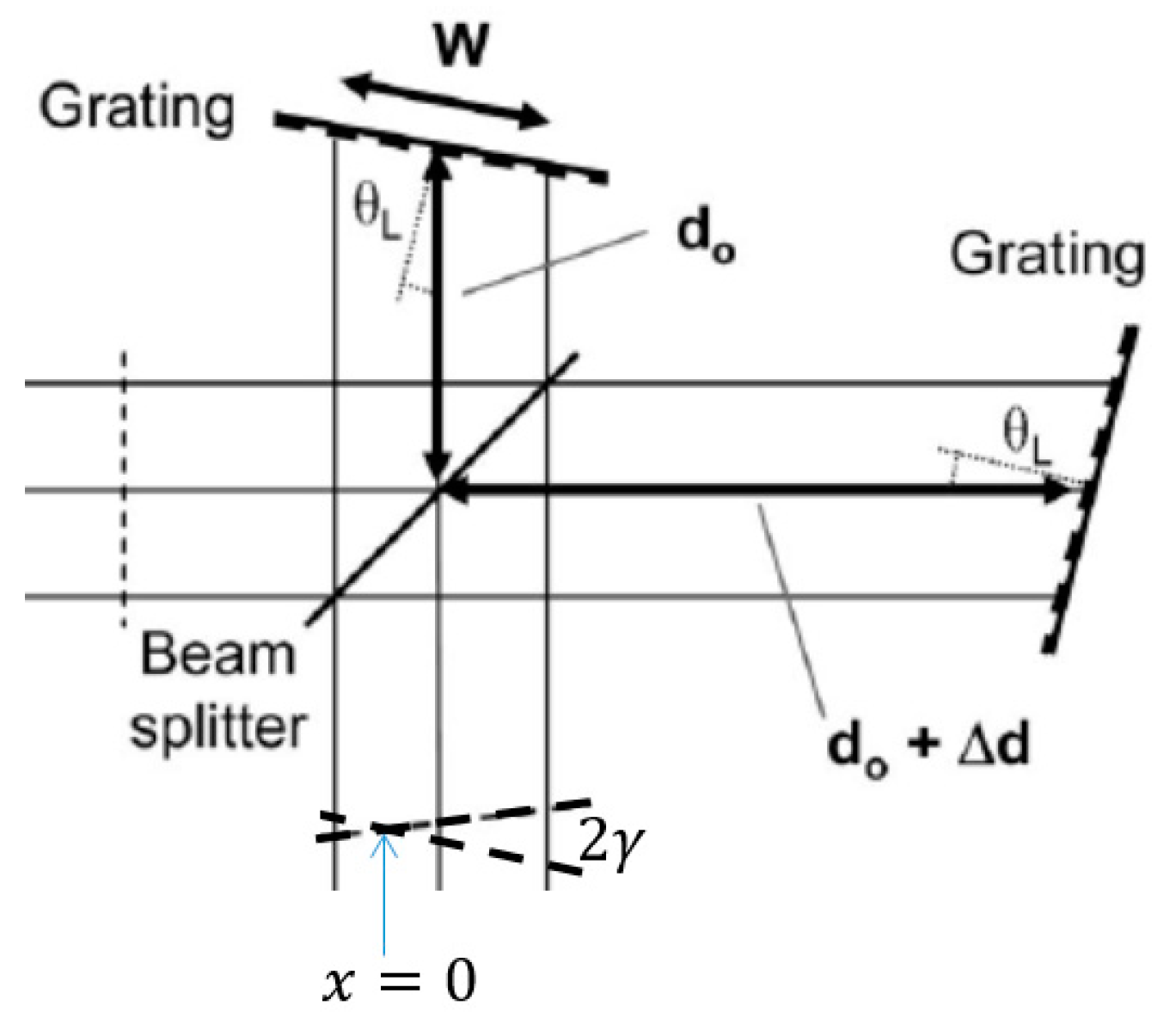
To alleviate the conflict between the effective pixel number N and spectral range $\mathsf{\Delta }{\sigma }_{\mathrm{eff}}$, the GMI-II introduces an asymmetric interferometric component design into the conventional SHS. As shown in Figure 6, by adjusting the distance between the grating of one arm and the beamsplitter from the original $d_0$ to $\mathsf{\Delta }d+d_0$, the ZOPD position is almost shifted from the optical axis position to the left side of the optical axis.

Compared to the conventional SHS, the range of the coordinates $x^{\prime }$ concerning the ZOPD and OPD $U^{\prime }$ in the dispersion direction is changed from Equation (5) to Equation (9).

$$\{\begin{array}{l}{x}^{\prime }\in \left[-\frac{1}{2}Wcos{\theta }_L+\frac{\mathsf{\Delta }d}{2tan{\theta }_L}, \frac{1}{2}Wcos{\theta }_L+\frac{\mathsf{\Delta }d}{2tan{\theta }_L}\right]\\ U^{\prime }\in \left[-Wsin{\theta }_L+\Delta d, Wsin{\theta }_L+\Delta d\right]\end{array}.$$

(9)

The expression for the maximum OPD ${U^{\prime }}_{\max }$ and spectral resolution interval $\delta {\sigma }^{\prime }$ is shown in Equation (10).

$$\{\begin{array}{l}{U^{\prime }}_{\max }=4{x^{\prime }}_{max}tan{\theta }_L=2Wsin{\theta }_L+2\Delta d\\ \delta {\sigma }^{\prime }=\frac{1}{2{U^{\prime }}_{\max }}==\frac{1}{4\left(Wsin{\theta }_L+\mathsf{\Delta }d\right)}\end{array}.$$

(10)

The asymmetric SHS effectively increases the spectral resolution interval of the instrument without changing the spectral range, as shown in Equation (11), while keeping the effective pixel number of the detector constant.

$$\Delta {\sigma }^{\prime }=\frac{1}{2}N\frac{Wsin{\theta }_L+\mathsf{\Delta }d}{Wsin{\theta }_L}\delta {\sigma }^{\prime }=\frac{N}{8Wsin{\theta }_L}=\Delta \sigma .$$

(11)

We can also expand the exit pupil diameter of the front system, increase the size of the object surface of the secondary imaging mirror group, and obtain the asymmetric interferogram only through the focal plane offset. Nevertheless, there are two problems caused by this: (1) energy loss; (2) the size of the interferometer and secondary imaging mirror group will expand. Based on the above considerations, we choose to change the centre thickness of the two arms’ field-widened prisms to carry out the bias design of ZOPD in the interferometer component of the main observation channel.

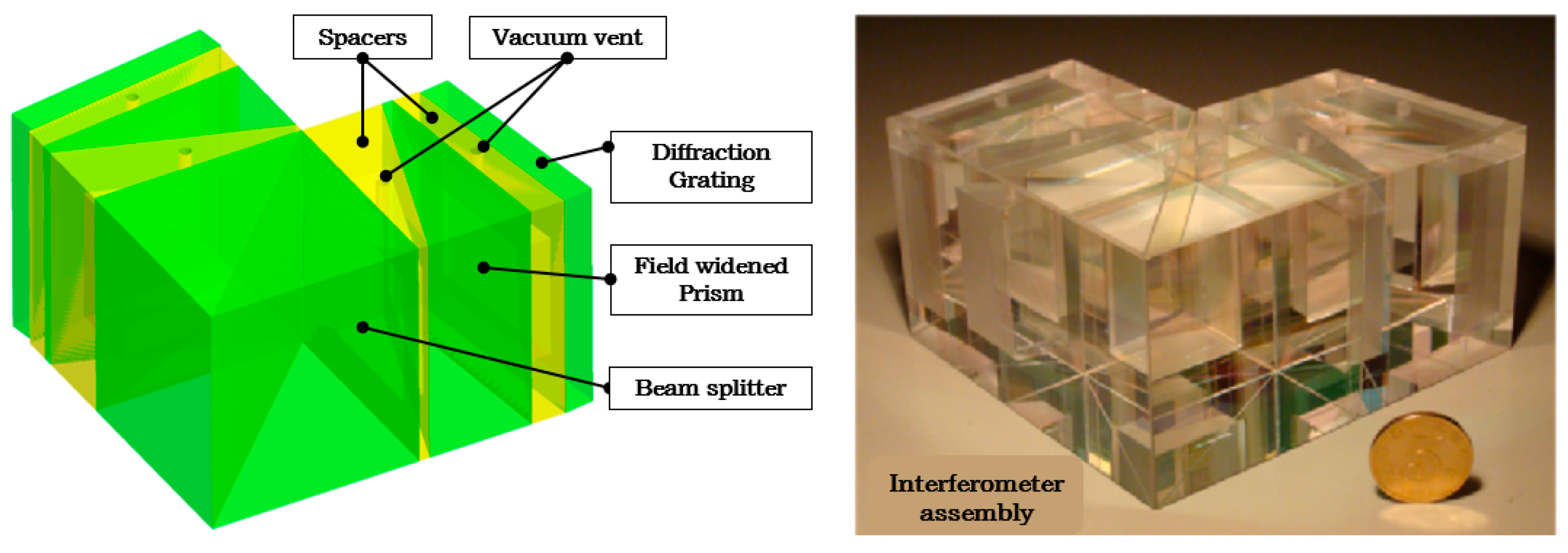
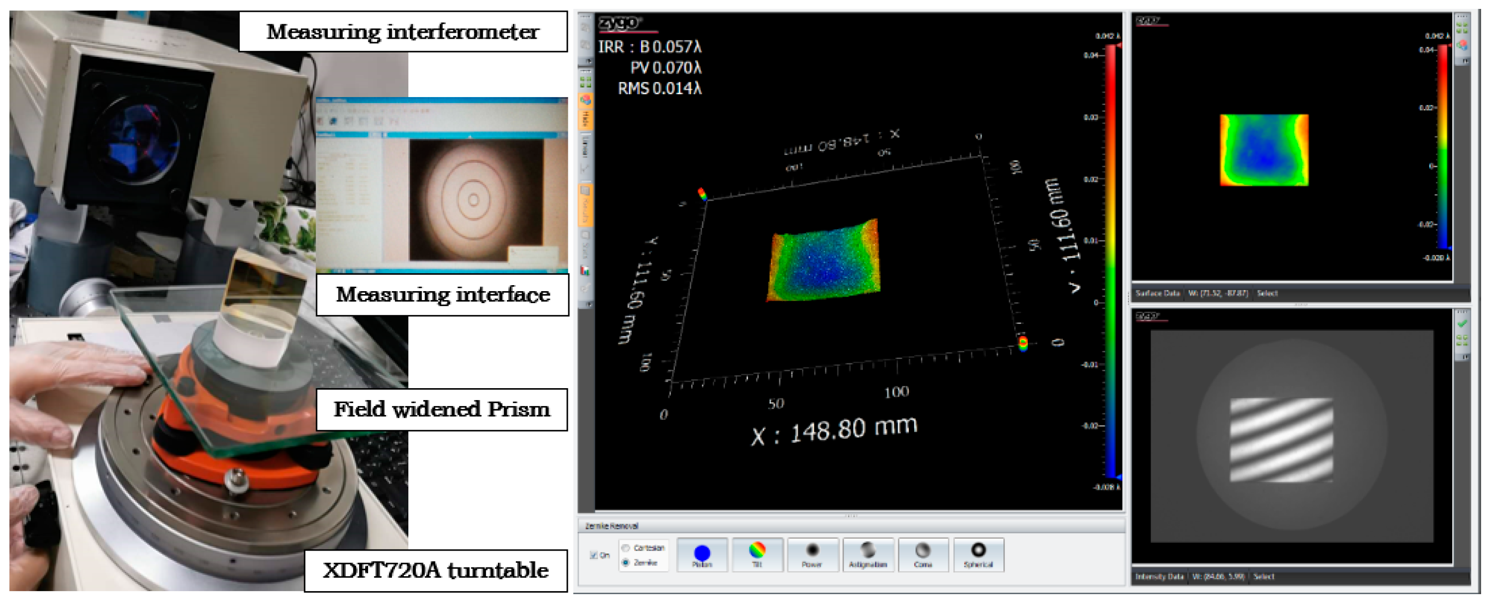
Compared to the air spacing thickness deviation $\mathsf{\Delta }d$, the thickness deviation of the field-widened optical wedge prisms is $\mathsf{\Delta }d/n$, where n is the refractive index of the field-widened prisms. Figure 7 shows the model diagram of the integrated glued interferometer assembly. The optical prisms and spacers with certain angles are glued together by optical glue, which can crack under the influence of external forces. Consequently, in order to enhance the spatial environmental adaptability of the integrated interferometer assembly, we used epoxy structural glue to bond glass cover plates of the same material on both the top and bottom of the interferometer assembly to prevent the loosening of the interferometer component due to stress changes in environmental conditions.

At the same time, the offset design of SHS cannot be carried out without restrictions. In addition to considering the spectral resolution requirements of the instrument, the ZOPD offset design is limited by the minimum sampling points of the short side past the ZOPD position of the interferogram. The instrument’s spectral resolution increases with offset, which is beneficial for fine spectra detection and high-precision concentration inversion for atmospheric GHG molecules. Nonetheless, phase errors, whose form factors are complex, are bound to exist in interferometric spectrometers, and the fewer the number of the short-side sampling points past the ZOPD position, the more difficult it is to correct the phase. Therefore, it is necessary to design the offset value of ZOPD reasonably. The parameters of the three main observation channels’ interferometers are shown in

Table 2. The parameters of asymmetric interferometers.

Specifications	Values
	CO2-1	CH4	CO2-2
Band range (nm)	1568–1583	1642–1658	2043–2058
Littrow wavelength (nm)	1564	1638.5	2038.5
Groove of grating (gr/mm)	450	450	300
Spectral dimension sampling point (pixel)	640	640	320
Field-widened prism material	F_SiLiCa	H-ZF88	H-ZF88
Thickness difference of field widened prism (mm)	1.30	1.20	1.80
Long side sampling point (pixel)	400	400	230
Proportion of short side to total sampling points	37.5%	37.5%	28.1%
$\delta {\sigma }^{\prime }$ of asymmetric SHS (cm−1)	0.218	0.217	0.220
Ratio of effective spectral bandwidth	69.1%	67.7%	70.4%

.

As can be seen from Table 2, we have chosen the sampling points of the short side past the ZOPD position of not less than 20% to meet the needs of phase correction on the one hand and to take into account the grating parameters, narrowband filters, primary technical specifications for the main observation channels to match the design as well as. The transmittance of the narrowband filters for the four channels is no more than 5% at the fundamental and spatial frequency cut-off wavelengths, and the transmittance of the effective spectral bandwidth should be as high as possible. It is worth noting that the accuracy requirement of the centre wavelength of the narrowband filter is less significant for the GMI-II than for conventional applications because each spectral absorption peak in this band is equally important for the inversion.

The above design not only meets the main specifications of the GMI-II, such as spectral resolution and effective spectral range, but also meets the constraints and limitations of the processing technology level of core components, such as blazing grating and narrowband filter. The final spectral resolution of the instrument is also related to the scaling ratio of the imaging system in the direction of the grating dispersion, i.e., the spectral dimension, as the scaling ratio is directly related to the size ${x^{\prime }}_{max}$ at the localisation plane of the interference fringe conjugate to the detector sensing plane.

2.4. Secondary Imaging System with Non-Isometric Scaling in the Meridian and Sagittal Planes

The role of the secondary imaging system is to scale the interference fringe in the localisation domain plane and to image it on the plane array detector. According to the parameters of the interferometer in Section 2.3 (the effective width of grating in the dispersion direction, interferometer field of view angle, interferometer optical material and size, etc.) and array detector parameters (spectral response curve, pixel number, pixel size, etc.), the observation channel design parameters of the imaging system is obtained.

The design inputs include the following four requirements: (1) the object plane height, i.e., the exiting pupil position and the size of the collimating unit; (2) the object space NA (Numerical Aperture), which contains the grating dispersion in the effective wavelength range; (3) the object space telecentric system, i.e., the input to the collimating system is a quasi-parallel beam; (4) a fixed scaling ratio in the dispersion direction. At the same time, it is required that the length of the four channels’ imaging system should be the same as possible because, in the thermal design scheme, the cooling and heat dissipation surface of the detector with four channels is transmitted to the whole satellite +Y plane through the same panel.

In the main observation channels, the low spectral response efficiency and the long integration time of the detector lead to excessive dark current. The secondary imaging system of the main observation channels was designed with energy compression along the grating groove direction, i.e., perpendicular to the dispersion direction, which effectively solves the problem that the signal energy is limited by the integration time, or the dark current is too large for the effective signal to be swamped.

The imaging system of the O₂ channel has the same scaling in the meridian plane (grating dispersion cross-section) and sagittal plane, both of which are −0.6208. At the same time, the imaging system should be designed to minimise geometric distortion as much as possible, which can generally be ignored at < 0.1%, and geometric distortion correction is not required for the interferometric image pre-processing process.

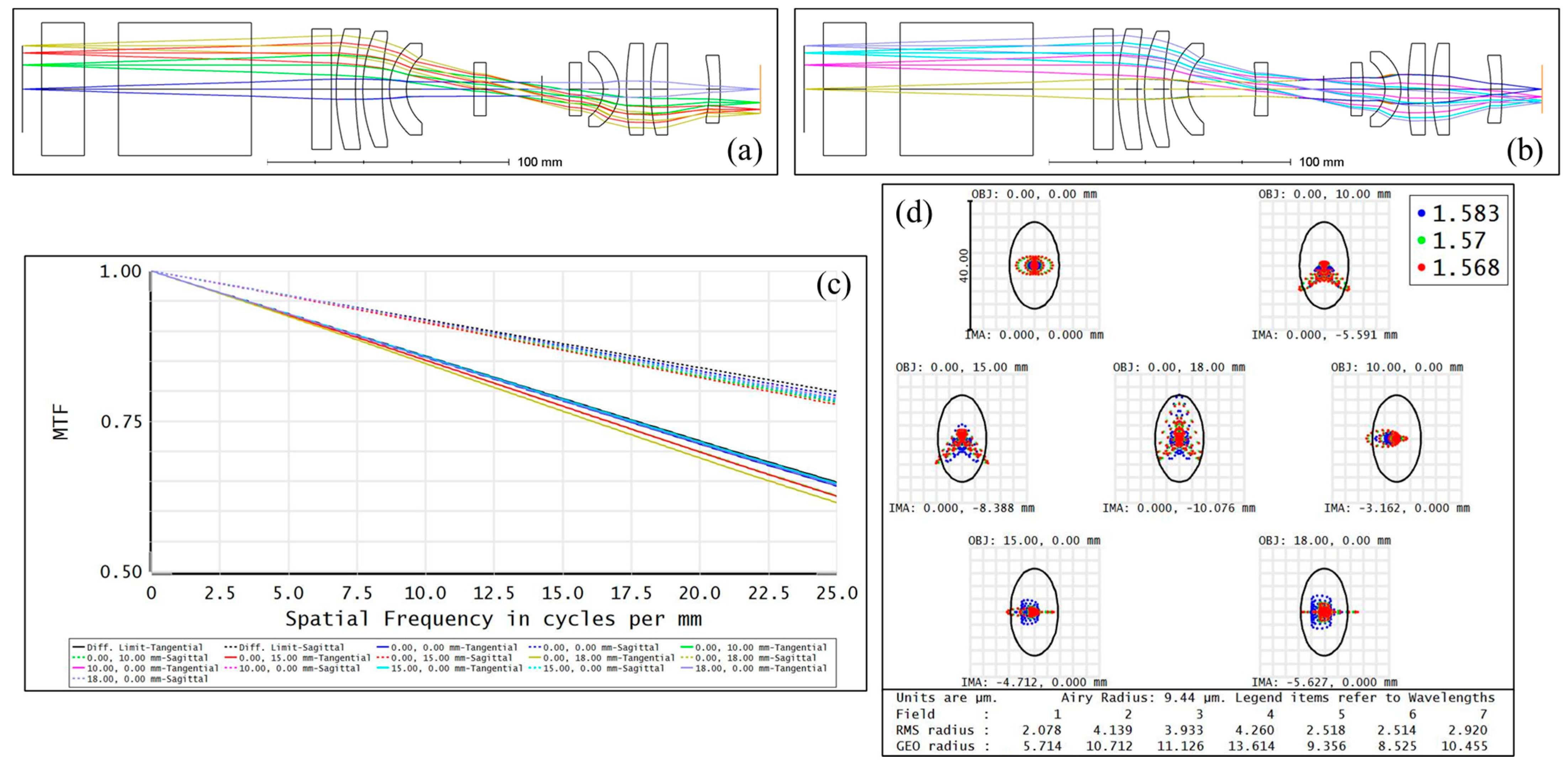
The imaging systems of the CO₂-2, CH₄ and CO₂-1 channels simultaneously achieve the effective sampling of the maximum OPD in the spectral dimension and energy compression in the spatial dimension. Figure 8a,b shows the CO₂-2 channel’s optical path diagrams of the grating and vertical dispersion direction, respectively. By using the curvature difference between the two mirrors of the middle image plane in the meridian plane and the sagittal plane, namely, the concave cylindrical mirror and convex cylindrical mirror, the different imaging ratios of spatial and spectral dimensions are realized, which are −0.5594 and −0.3108 respectively.

Correspondingly, the diffraction limits of the meridian and sagittal planes are different, as shown in Figure 8c at the detector Nyquist sampling frequency of 25.0 lp/mm, where the corresponding MTF in the meridian and sagittal planes reaches 0.65 and 0.80, respectively. The Airy spot also exhibits an elliptical shape, as shown in Figure 8d. It should be noted that the relative distortion of the spectral dimension is better than 0.1%, and that of the spatial dimension is about 2% as far as possible. Therefore, the relative distortion of spatial dimension needs to be corrected in the subsequent data processing. The design results of imaging systems are shown in

Table 3. Design results of the imaging systems.

Specifications	Values
	O2	CO2-1	CH4	CO2-2
Band range (nm)	759–769	1568–1583	1642–1658	2043–2058
Height of object space (mm)	34	35	35	34
Scaling ratio in the spectral dimension	−0.6208	−0.5594	−0.5519	−0.4430
Energy compression ratio in spatial dimensional	$\frac{-0.6208}{1.00}$	$\frac{-0.5594}{1.80}$	$\frac{-0.5519}{1.80}$	$\frac{-0.4430}{1.90}$
Secondary imaging system length (mm)	285	297	297	297

.

3. Fabrication and Alignment

3.1. Telescopic System Test

The telescope system was tested using the Shack-Hartmann wavefront sensor, and the alignment layout is shown in Figure 9. The light emitted from the Shack-Hartmann wavefront sensor is modulated by the primary mirror of the telescope system, the field stop, and the secondary mirror into parallel light emitted to the observation window at the end of the primary mirror. Then the parallel emitted light was reflected by the reflector, returned along the original optical path, and finally received by the sensor, which dynamically monitored the alignment state of the primary and secondary mirrors through the interference wavefront. As shown on Figure 10, the exiting wavefront of the axial light of the telescope system after accurate alignment is better than 0.1 waves @ 632.8 nm, which is equivalent to the design result.

3.2. Non-Isometric Compression Secondary Imaging System Test

Under the illumination in the specific field angle and spectral band, the standard plate on the measured object plane can be clearly imaged in the effective spectral band using the detector. Through data processing, the scaling ratio and limit resolution of the secondary imaging system are calculated.

The test layout is shown in Figure 11, and the test process is as follows: (a) the integrating sphere light source is selected, and the distance between the integrating sphere and the secondary imaging system is adjusted so that the illumination meets the requirements of the secondary imaging system object space NA; (b) adjust the consistency of the normal direction of the discriminant plate, the optical axis of the measured secondary imaging system (including the filter) and the normal direction of the detector’s photosensitive surface, and the discriminant plate is located in the object distance as described in

Table 4. Requirements for the testing parameters of the secondary imaging systems of the four channels.

Index		O2	CO2-2	CH4	CO2-1
Object distance (mm)		77.5	86.9	85.2	90.3
Scaling ratio	Spectral dimension	0.6209	0.4436	0.5927	0.5595
	Spatial dimension	0.6209	0.2361	0.3282	0.3131
Resolution (lp/mm)	Spectral dimension	23.88	7.39	14.82	14.3
	Spatial dimension	23.88	3.93	8.21	8.00
Detector parameters		1024 × 1024 @ 13 μm	320 × 256 @ 30 μm	640 × 512 @ 20 μm

; (c) adjust the position of the detector relative to the secondary imaging system on the optical axis so that it can image the most clearly on the discriminator plate, collect the imaging data, and record the dark current data at the corresponding integration time; (d) carry out data processing, and calculate the scaling ratio and limit resolution of the secondary imaging system listed in

Table 5. List of measured results of the imaging systems of the four channels.

Index		O2	CO2-2	CH4	CO2-1
Square nominal value (mm)		2.228
Spectral dimension	Measured pixel number	106 (13 μm)	33.5 (30 μm)	65.5 (20 μm)	63 (20 μm)
	Measured scaling ratio	0.6185	0.4511	0.5880	0.5655
	Ratio error	0.39%	1.69%	0.80%	1.08%
	Resolution (lp/mm)	25.4	7.13	14.3	16.0
Spectral dimension	Measured pixel number	106 (13 μm)	17.5 (30 μm)	38 (20 μm)	35.5 (20 μm)
	Measured scaling ratio	0.6185	0.2356	0.3411	0.3187
	Ratio error	0.39%	0.20%	3.93%	1.78%
	Resolution (lp/mm)	25.4	4.49	8.98	8.00

.

During the test, the size and number of the test detector are consistent with the parameters of the GMI-II photographic chip. The diameter D of the integrating sphere and the distance L between the integrating sphere and the object surface of the imaging system should satisfy the equivalent object space NA of the secondary imaging system. The narrowband filter of each channel is located between the standard plate and the secondary imaging system, and the USAF-1951 bar target on the object surface is installed in the test fixture of each channel imaging system.

3.3. Single-Channel Spectrometer Alignment and Assembly

After the collimation and imaging systems are assembled, the interferometer can be glued and tested. The interferometer assembly comprises several optical prisms with particular angles accuracy better than 2″ and prism spacers. The surface accuracy of individual optical elements should be better than 0.5 fringes, and the local irregularity should be better than 0.2 fringes (@ 633 nm) to ensure the quality and angular accuracy of the adhesive. Figure 12 shows the angular measurement process and face shape test result of a field-widened prism. The angular measurement was performed with a multi-tooth dividing turntable with 0.2″ angular accuracy combined with an interferometer.

Each channel interferometer uses semi-customised grating. We commission the fabrication of grating substrates of specific materials and sizes, and then the grating manufacturer replicates it as required. To reduce the polarisation sensitivity of the GMI-II, we used a beamsplitter prism with equal proportion and non-polarising, and gratings with similar TE/TM diffraction efficiency.

During the glueing process, we only adjusted the grating tilt angle, used polychromatic light illumination to obtain interferograms and recovered the spectrum to determine whether the spectral response curve covered the effective spectral range, i.e., the number of spectral sampling points for low and high-frequency aliasing was as equal as possible.

The focal plane of the single-channel spectrometer is adjusted after the grating has been glued, including the optimum image plane adjustment in the direction of the optical axis, the adjustment of the focal plane rows/columns with respect to the grating groove direction, and the adjustment of the interferometric ZOPD position in the column position on the focal plane. Considering a certain amount of defocusing in a vacuum environment, the adjustment shims are selected in favour of the optimum shim thickness in the vacuum. The spacers are made of polyimide or fibreglass and hollowed out to minimise heat exchange between the imaging system and the focal plane assembly.

3.4. GMI-II Optical Unit Alignment

The alignment of the optics machine head is mainly the alignment of the optical unit, including the following contents.

(1) The telescope system’s alignment includes field stop and field test alignment. The optical axis reference plane of the GMI-II is located within the range of φ200 mm near the optical inlet, of which φ110 mm is the through-optical aperture.

(2) The collimating and secondary imaging systems were centring aligned, and the secondary imaging systems were tested for MTF, scaling ratio and other major performance indicators.

(3) Single-channel spectrometer alignment, including interferometer assembly grating glueing, optimal image plane position alignment and consistency adjustment of image plane row/column and grating groove direction, etc.

(4) The four channels’ spectrometers and telescope systems can be effectively spliced using dichroic reflectors. In the process of dichroic reflector adjustment, four channels are needed to coordinate the adjustment. The lift of the optical axis caused by the angle and thickness of the dichroic reflectors will affect the FOV and light-passing state of subsequent optical paths. The optimal condition is when the dichroic reflectors are adjusted to the maximum average Digital Number (DN) value of the focal plane. In practice, we use average DN and interference modulation to evaluate the alignment process comprehensively.

(5) After testing each of the above functional components, thermal control is implemented, including the adhesion of the heating pad and thermistor.

(6) Finally, the optical and calibration units (including the 2D tracking mirror, diffuse reflector plate, calibration gate, etc.) are assembled. The calibration of the sub-satellite point of the 2D tracking mirror in the calibration unit is completed, i.e., the optical axis of the optical unit is transferred to the X and Y axis motor fixed coding values of the 2D tracking mirror.

4. Performance Parameter Test and Calibration

This section focuses on the spectral calibration results for spectral resolution, spectral range, central wavelength, and other technical specifications of the GMI-II optics machine head. The SNR of the GMI-II is evaluated and tested under the typical radiance of the GMI-I statistics in orbit for two years. According to the observation data of the GMI-II in orbit, the GHG inversion test was carried out.

4.1. Spectral Calibration

The spectral calibration test of the GMI mainly includes the detection of the payload’s spectral resolution, spectral range, central wavelength and other indicators, which are detected by utilising a tunable laser (± 5 pm wavelength accuracy). The interferogram obtained from the SHS is Fourier transformed to obtain the spectral data [39]. Assuming that the bilinear spectra are ${\lambda }_1, {\lambda }_2 ({\lambda }_1>{\lambda }_2)$, respectively, the coordinates of the Fourier transformed spectral point are $x_1, x_2$, respectively. According to the pixel number $N_{fwhm}$ of FWHM, the system parameters can be calculated. If there are more than two spectral lines, the spectral lines can verify the system parameters with each other. The parameters are calculated as follows.

• Sampling resolution $\delta {\lambda }_1$: $\delta {\lambda }_1=\left({\lambda }_1-{\lambda }_2\right)/\left|x_1-x_2\right|$;
• Spectral resolution $\delta {\lambda }_2$: $\delta {\lambda }_2=\delta {\lambda }_1\cdot N_{fwhm}$;
• Spectral range $\mathsf{\Delta }\lambda$: $\mathsf{\Delta }\lambda ={\lambda }_{max}-{\lambda }_{min}$, where ${\lambda }_{max}={\lambda }_2-x_2·\delta {\lambda }_1$ and ${\lambda }_{min}={\lambda }_2+\left(1024-x_2\right)\delta {\lambda }_1$.

A spectral resolution test set-up is constructed using a tunable laser (± 5 pm wavelength accuracy), homogeneous integrating sphere, wavelength meter and power meter. The laser emits a monochromatic spectrum, which is introduced into the integrating sphere to form a uniform, quasi-Lambert surface light source at the exit. The wavelength and power meters are used to monitor the wavelength and power of the laser output. By collecting monochromatic interferograms of different wavelengths, spectral restoration was performed to obtain the instrument’s linear shape (ILS) at different wavelengths, and spectral resolution values were obtained after measuring FWHM values [40]. The monochromatic light recovery spectra and spectral calibration fit results of the CO₂-1 channel are shown in Figure 13. The spectral resolution of the CO₂-1 channel varies from 0.260 to 0.268 cm⁻¹.

The CO₂-2 channel test requires the detector to be heat-sink cooled to ensure that the focal plane of the channel is stable at 185 K. Therefore, the channel is placed in a vacuum tank with a fused quartz glass window, which the integrating sphere or monochromatic light is incident on the instrument through. The angle of the scanning mirror is adjusted so that the channel can be uniformly illuminated. The spectral calibration results for each channel are shown in

Table 6. Spectral calibration results for each channel.

Channel	Required Value (cm−1)	Measured Value (cm−1)	Uncertainty (cm−1)
O2	≤0.6	0.582	0.0083
CO2-1	≤0.27	0.263	0.0089
CH4	≤0.27	0.262	0.0112
CO2-2	≤0.27	0.268	0.0044

. The spectral calibration uncertainty in Table 6 is determined by the following factors: (1) uncertainty in the output wavelength of the laser, quoting product parameter data; (2) uncertainty in the regression analysis containing the spectral recovery uncertainty and the peak localisation uncertainty, estimated using the standard deviation of the residuals.

As seen in Table 6, the spectral resolution of each channel meets the requirement of technical indicators, and the spectral calibration uncertainty is better than 0.05 cm⁻¹. The spectral range is not listed in the table because the spectral range needs to meet the requirement of the SNR. It will be described after the SNR test is completed.

4.2. Absolute Radiometric Calibration

Absolute radiometric calibration mainly establishes a quantitative relationship between the instrument’s output signal and the input spectral radiance. The GMI-II uses an integrating sphere radiometric calibration system characterised by high output energy, excellent surface uniformity and angular properties (Lambertianity). The integrating sphere with a diameter of 3 m is used to simulate the brightness change of the incident pupil by changing the current or lamp number in the integrating sphere, representing different surface reflectance during earth observation. The GMI-II observes the radiation source of the integrating sphere and acquires interferograms and dark background data.

The absolute radiometric calibration process is as follows. First of all, a standard lamp with a known spectral radiance is needed to calibrate the radiance of the integrating sphere. By transferring the spectral radiance of the standard lamp to the integrating sphere, the spectral radiance at the opening of the integrating sphere is calibrated, and then the integrating sphere is used to calibrate the radiance to the calibration payload.

The absolute radiometric calibration accuracy is determined by: (1) the absolute radiometric uncertainty $u\left(a\right)$ of the integrating sphere radiation source, quoting product parameters; (2) non-stability $\overline{u\left(b\right)}$ of the payload and (3) spectral response non-linearity $\overline{u\left(l\right)}$ of the payload. Multiple measurements of the integrating sphere radiation source under the same conditions were used to perform spectral recovery of the interferogram and to assess the stability and spectral response linearity of the spectral points. Figure 14 shows the spectral data stability and spectral response of the CO₂-1 channel. The calculation of the non-stability $u{(b)}_{\lambda }$ and spectral response non-linearity $u{(l)}_{\lambda }$ at wavelength $\lambda$ is shown in Equation (12).

$$\{\begin{array}{c}u{(b)}_{\lambda }=\frac{1}{\langle Y\left(\lambda \right)\rangle }\sqrt{\frac{{{\displaystyle \sum }}_{t=1}^T{[Y\left(\lambda ,t\right)-\langle Y\left(\lambda ,t\right)\rangle ]}^2}{T-1}}\times 100\%\\ u{(l)}_{\lambda }=\left[\frac{RMSE\left(\lambda \right)}{\langle Y\left(\lambda \right)\rangle }\right]\times 100\%\end{array}.$$

(12)

The non-stability $\overline{u\left(b\right)}$ and spectral response non-linearity $\overline{u\left(l\right)}$ of the payload are the mean value of $u{(b)}_{\lambda }$ and $u{(l)}_{\lambda }$ in the effective spectral range, respectively. The absolute radiometric calibration accuracy for all four channels of the GMI-II is better than 5%, as shown in

Table 7. Absolute radiometric calibration accuracy for each channel of the GMI-II.

Uncertainty Factor	O2	CO2-1	CH4	CO2-2
Integrating sphere radiometric uncertainty $u\left(a\right)$	2.30%	2.74%	2.71%	3.90%
Non-stability $\overline{u\left(b\right)}$	0.13%	0.26%	0.08%	0.18%
Spectral response non-linearity $\overline{u\left(l\right)}$	0.38%	0.43%	0.62%	0.90%
Absolute radiometric calibration accuracy	2.33%	2.79%	2.78%	4.01%

.

4.3. SNR Test

The GMI-II performed the vacuum tank’s performance test on 26 March 2020. The radiance of two years’ on-orbit observation data of the same type of payloads in the world was comprehensively analysed, as shown in

Table 8. Statistical radiance on-orbit observation and required radiance of the GMI-II.

Channel	Statistical Radiance	Required Radiance
O2	42 W/(m2⋅sr⋅μm)	60 W/(m2⋅sr⋅μm)
CO2-1	10 W/(m2⋅sr⋅μm)	20 W/(m2⋅sr⋅μm)
CH4	10 W/(m2⋅sr⋅μm)	20 W/(m2⋅sr⋅μm)
CO2-2	3 W/(m2⋅sr⋅μm)	8 W/(m2⋅sr⋅μm)

. The required radiance is calculated under the condition that albedo = 0.3 and sun elevation = 30°. Figure 15 shows the SNR test results of the GMI-II at statistical and required irradiance. The average SNR of the GMI-II at the required radiance is better than the performance specifications in Table 1, as shown in

Table 9. The average SNR test results of the GMI-II at the required radiance.

Channel	Required Spectral Range	Effective Spectral Range	Average SNR
O2	759–769 nm	758–770 nm	887
CO2-1	1568–1583 nm	1569–1584 nm	1082
CH4	1642–1658 nm	1641–1659 nm	853
CO2-2	2043–2058 nm	2042.5–2059 nm	492

.

After the thermal vacuum and thermal equilibrium tests, the stability of the GMI-II was tested using a dedicated ground-check light source, as shown in

Table 10. Comparison of ground-checked light source results.

Time	B1			B4			B3
	DN	Dark	ZOPD	DN	Dark	ZOPD	DN	Dark	ZOPD
Pre-test	10,717	1235	501	7945	714	236	5410	1132	406
Post-test	10,669	1247	501	7871	721	237	5359	1135	406
Rate of change	0.45%	−0.96%	0.0	0.94%	−0.97%	1.0	0.95%	−0.26%	0.0

. The ZOPD position offset changes in a pixel before and after the test, which indicates that the micro-stress state of the interferometer installation and glueing is good. The change in DN value may be caused by repeated positioning errors of the ground-check light source installed before and after the test because only two M6 screws are used for the light source and GMI-II without the positioning pin structure. However, the change in DN value before and after the test was still within 1%.

4.4. In-Orbit Data Testing

The GMI-II observation data from 25 October to 2 November 2021 were used to carry out the inversion tests for column-averaged dry-air mole fraction of CO₂ and CH₄ (XCO₂ and XCH₄). The inversion calculation method uses the best estimate method [41].

The XCO₂ inversion sites of the GMI-II have 869 sites on a global scale. The global mean value of XCO₂ from the GMI-II is 413.41 ppm, corresponding to a regional mean value of 413.38 ppm for the GOSAT XCO₂ product. The mean values of CO₂ concentrations detected by the GMI-II and GOSAT are consistently high, and the trend in the global distribution of CO₂ concentrations is consistent, as shown in Figure 16.

The XCH₄ inversion sites of the GMI-II have 886 sites on a global scale. The global mean value of XCH₄ from the GMI-II is 1.8879 ppm, corresponding to a regional mean value of 1.8946 ppm for the GOSAT XCH₄ product. The mean CH₄ concentrations detected by the GMI-II are slightly higher than those detected by the GOSAT, and the global distribution of CH₄ concentrations follows the same trend, as shown in Figure 17.

The global trends of XCO₂ and XCH₄ from the GMI-II observations are in good agreement with the GOSAT. The average deviation of XCO₂ detected by the GMI-II compared to the GOSAT was 0.16 ppm with a standard deviation of 0.52%, which is better than the 1% accuracy requirement. The average deviation of XCH₄ detected by the GMI-II compared to the GOSAT was 0.0022 ppm with a standard deviation of 1.16%, which is better than the 2% accuracy requirement.

5. Conclusions

The GMI-II was designed and developed for quantitative remote sensing monitoring of the main GHG in the atmosphere. The main performance parameters of the GMI-II have been tested in the laboratory, which proves the effectiveness of quantitative monitoring of GHG column concentrations. The interferometer assembly with ZOPD position offset has been designed optimally to improve the spectral resolution by more than 20% while keeping the number of the detector’s pixels in the spectral dimension unchanged. The secondary imaging system is designed to compress the energy in the spatial dimension, which can increase the energy of a single pixel and improve the spectral SNR of a single-frame interferogram within a limited integration time.

References

1. Bruhwiler, L.; Basu, S.; Butler, J.H.; Chatterjee, A.; Dlugokencky, E.; Kenney, M.A.; McComiskey, A.; Montzka, S.A.; Stanitski, D. Observations of greenhouse gases as climate indicators. Clim. Chang. 2021, 165, 12. [Google Scholar] [CrossRef] [PubMed]
2. Betts, A.K.; Ball, J.H.; Beljaars, A.; Miller, M.J.; Viterbo, P.A. The land surface-atmosphere interaction: A review based on observational and global modeling perspectives. J. Geophys. Res.-Atmos. 1996, 101, 7209–7225. [Google Scholar] [CrossRef] [Green Version]
3. Manabe, S.; Wetherald, R.T. Distribution of Climate Change Resulting from an Increase in CO2 Content of the Atmosphere. J. Atmos. Sci. 1980, 37, 99–118. [Google Scholar] [CrossRef]
4. IPCC. Global Warming of 1.5 °C: IPCC Special Report on Impacts of Global Warming of 1.5 °C above Pre-industrial Levels in Context of Strengthening Response to Climate Change, Sustainable Development, and Efforts to Eradicate Poverty; IPCC: Cambridge, UK, 2022. [Google Scholar]
5. Liu, Z.; Deng, Z.; Davis, S.J.; Giron, C.; Ciais, P. Monitoring global carbon emissions in 2021. Nat. Rev. Earth Environ. 2022, 3, 217–219. [Google Scholar] [CrossRef] [PubMed]
6. Calvo Buendia, E.; Tanabe, K.; Kranjc, A.; Baasansuren, J.; Fukuda, M.; Ngarize, S.; Osako, A.; Pyrozhenko, Y.; Shermanau, P.; Federici, S. 2019 Refinement to the 2006 IPCC Guidelines for National Greenhouse Gas Inventories; IPCC: Geneva, Switzerland, 2019; ISBN 978-4-88788-232-4. [Google Scholar]
7. Breon, F.M.; Ciais, P. Spaceborne remote sensing of greenhouse gas concentrations. Comptes Rendus Geosci. 2010, 342, 412–424. [Google Scholar] [CrossRef]
8. Wunch, D.; Toon, G.C.; Blavier, J.; Washenfelder, R.A.; Notholt, J.; Connor, B.J.; Griffith, D.; Sherlock, V.; Wennberg, P.O. The Total Carbon Column Observing Network. Philos. Trans. R. Soc. A-Math. Phys. Eng. Sci. 2011, 369, 2087–2112. [Google Scholar] [CrossRef] [Green Version]
9. Palmer, P.I. Quantifying sources and sinks of trace gases using space-borne measurements: Current and future science. Philos. Trans. R. Soc. A-Math. Phys. Eng. Sci. 2008, 366, 4509–4528. [Google Scholar] [CrossRef]
10. Mao, J.; Kawa, S.R. Sensitivity studies for space-based measurement of atmospheric total column carbon dioxide by reflected sunlight. Appl. Opt. 2004, 43, 914–927. [Google Scholar] [CrossRef]
11. Zhang, X.; Wang, F.; Wang, W.; Huang, F.; Chen, B.; Gao, L.; Wang, S.; Yan, H.; Ye, H.; Si, F.; et al. The development and application of satellite remote sensing for atmospheric compositions in China. Atmos. Res. 2020, 245, 105056. [Google Scholar] [CrossRef]
12. Obland, M.D.; Corbett, A.M.; Lin, B.; Meadows, B.; Campbell, J.F.; Kooi, S.; Fan, T.F.; Carrion, W.; Hicks, J.; Sparrow, J.; et al. Advancements towards active remote sensing of CO2 from space using Intensity-Modulated, Continuous-Wave (IM-CW) lidar. In Sensors, Systems, and Next-Generation Satellites XXII; SPIE: Bellingham, WA, USA, 2018. [Google Scholar]
13. Allan, G.R.; Abshire, J.B.; Stephen, M.A.; Ramanathan, A.; Riris, H.; Hasselbrack, W.; Chen, J.; Yu, A.; Sung, X.L.; Numata, K.; et al. CO2 Sounder Lidar Development at NASA-GSFC for the ASCENDS Mission. In Proceedings of the Conference on Lasers and Electro-Optics: Science and Innovations 2016, San Jose, CA, USA, 5–10 June 2016; p. STh1H.3. [Google Scholar] [CrossRef]
14. Caron, J.; Durand, Y. Operating wavelengths optimization for a spaceborne lidar measuring atmospheric CO2. Appl. Opt. 2009, 48, 5413–5422. [Google Scholar] [CrossRef]
15. Crisp, D.; Pollock, H.R.; Rosenberg, R.; Chapsky, L.; Lee, R.; Oyafuso, F.A.; Frankenberg, C.; O’Dell, C.W.; Bruegge, C.J.; Doran, G.B.; et al. The on-orbit performance of the Orbiting Carbon Observatory-2 (OCO-2) instrument and its radiometrically calibrated products. Atmos. Meas. Tech. 2017, 10, 59–81. [Google Scholar] [CrossRef] [Green Version]
16. Basilio, R.R.; Bennett, M.W.; Eldering, A.; Lawson, P.R.; Rosenberg, R.A. Orbiting Carbon Observatory-3 (OCO-3) remote sensing from the International Space Station (ISS). In Sensors, Systems, and Next-Generation Satellites XXIII; SPIE: Bellingham, WA, USA, 2019. [Google Scholar]
17. Eldering, A.; Taylor, T.E.; O’Dell, C.W.; Pavlick, R. The OCO-3 mission: Measurement objectives and expected performance based on 1 year of simulated data. Atmos. Meas. Tech. 2019, 12, 2341–2370. [Google Scholar] [CrossRef] [Green Version]
18. Liu, Y.; Wang, J.; Yao, L.; Chen, X.; Cai, Z.N.; Yang, D.X.; Yin, Z.S.; Gu, S.Y.; Tian, L.F.; Lu, N.M.; et al. The TanSat mission: Preliminary global observations. Sci. Bull. 2018, 63, 1200–1207. [Google Scholar] [CrossRef] [PubMed] [Green Version]
19. Yang, D.X.; Liu, Y.; Feng, L.; Wang, J.; Yao, L.; Cai, Z.N.; Zhu, S.H.; Lu, N.M.; Lyu, D.R. The First Global Carbon Dioxide Flux Map Derived from TanSat Measurements. Adv. Atmos. Sci. 2021, 38, 1433–1443. [Google Scholar] [CrossRef]
20. Veefkind, J.P.; Aben, I.; McMullan, K.; Forster, H.; de Vries, J.; Otter, G.; Claas, J.; Eskes, H.J.; de Haan, J.F.; Kleipool, Q.; et al. TROPOMI on the ESA Sentinel-5 Precursor: A GMES mission for global observations of the atmospheric composition for climate, air quality and ozone layer applications. Remote Sens. Environ. 2012, 120, 70–83. [Google Scholar] [CrossRef]
21. Nakajima, M.; Suto, H.; Yotsumoto, K.; Shiomi, K.; Hirabayashi, T. Fourier transform spectrometer on gosat and gosat-2. In International Conference on Space Optics—ICSO 2014; SPIE: Bellingham, WA, USA, 2014. [Google Scholar]
22. Nakajima, M.; Kuze, A.; Suto, H. The current status of GOSAT and the concept of GOSAT-2. In Sensors, Systems, and Next-Generation Satellites XVI; SPIE: Bellingham, WA, USA, 2012. [Google Scholar]
23. Zhang, P.; Lu, Q.F.; Hu, X.Q.; Gu, S.Y.; Yang, L.; Min, M.; Chen, L.; Xu, N.; Sun, L.; Bai, W.G.; et al. Latest Progress of the Chinese Meteorological Satellite Program and Core Data Processing Technologies. Adv. Atmos. Sci. 2019, 36, 1027–1045. [Google Scholar] [CrossRef]
24. Jervis, D.; McKeever, J.; Durak, B.; Sloan, J.J.; Gains, D.; Varon, D.J.; Ramier, A.; Strupler, M.; Tarrant, E. The GHGSat-D imaging spectrometer. Atmos. Meas. Tech. 2021, 14, 2127–2140. [Google Scholar] [CrossRef]
25. Wang, Q.S.; Luo, H.Y.; Li, Z.W.; Shi, H.L.; Ding, Y.; Xiong, W. Research progress of greenhouse gases spaceborne passive remote sensing detection payload. Natl. Remote Sens. Bull. 2023, 27, 1–14. [Google Scholar] [CrossRef]
26. Xiong, W. Greenhouse gases Monitoring Instrument (GMI) on GF-5 satellite (invited). Infrared Laser Eng. 2019, 48, 303002. [Google Scholar] [CrossRef]
27. Xiong, W. Hyperspectral Greenhouse Gases Monitor Instrument (GMI) for Spaceborne Payload. Spacecr. Recovery Remote Sens. 2018, 39, 14–24. [Google Scholar]
28. Yoshida, Y.; Ota, Y.; Eguchi, N.; Kikuchi, N.; Nobuta, K.; Tran, H.; Morino, I.; Yokota, T. Retrieval algorithm for CO2 and CH4 column abundances from short-wavelength infrared spectral observations by the Greenhouse gases observing satellite. Atmos. Meas. Tech. 2011, 4, 717–734. [Google Scholar] [CrossRef] [Green Version]
29. Butz, A.; Guerlet, S.; Hasekamp, O.; Schepers, D.; Galli, A.; Aben, I.; Frankenberg, C.; Hartmann, J.M.; Tran, H.; Kuze, A.; et al. Toward accurate CO2 and CH4 observations from GOSAT. Geophys. Res. Lett. 2011, 38, L14812:1–L14812:6. [Google Scholar] [CrossRef] [Green Version]
30. Bril, A.; Maksyutov, S.; Belikov, D.; Oshchepkov, S.; Yoshida, Y.; Deutscher, N.M.; Griffith, D.; Hase, F.; Kivi, R.; Morino, I.; et al. EOF-based regression algorithm for the fast retrieval of atmospheric CO2 total column amount from the GOSAT observations. J. Quant. Spectrosc. Radiat. Transf. 2017, 189, 258–266. [Google Scholar] [CrossRef] [Green Version]
31. Zhang, C.M.; Liu, D.D.; Rong, P.; Li, Y.F. Selection of Greenhouse gases Monitoring Instrument channels for CO2 in near infrared band. Optik 2017, 144, 597–602. [Google Scholar] [CrossRef]
32. Shi, H.L.; Li, Z.W.; Ye, H.H.; Luo, H.Y.; Xiong, W.; Wang, X.H. First Level 1 Product Results of the Greenhouse Gas Monitoring Instrument on the GaoFen-5 Satellite. IEEE Trans. Geosci. Remote Sens. 2021, 59, 899–914. [Google Scholar] [CrossRef]
33. Xiong, W. Optimum Design and Data Analysis of Greenhouse Gases Monitoring Instrument on GF-5 Satellite. Aerosp. Shanghai. 2019, 36, 167–172. [Google Scholar]
34. Luo, H.; Li, S.; Shi, H.; Xiong, W.; Hong, J. Optical design of imaging system based on spatial heterodyne spectrometer. Hongwai yu Jiguang Gongcheng/Infrared Laser Eng. 2016, 45, 818005. [Google Scholar]
35. Luo, H.; Xiong, W.; Shi, H.; Li, Z. Study for Signal-to-Noise Ratio of Spatial Heterodyne Spectrometer. Guangxue Xuebao/Acta Opt. Sin. 2017, 37, 0612001. [Google Scholar]
36. Luo, H.; Ye, Q.; Xiong, W.; Li, Z.; Li, S.; Shi, H. Study on the interferogram modulation efficiency of spatial heterodyne spectrometer. Guangxue Xuebao/Acta Opt. Sin. 2016, 36, 0712003:1–0712003:8. [Google Scholar]
37. Li, Z.W.; Xiong, W.; Shi, H.L.; Luo, H.Y.; Qiao, Y.L. Study on Asymmetric Spatial Heterodyne Spectroscopy. Spectrosc. Spectr. Anal. 2016, 36, 2291–2295. [Google Scholar]
38. Luo, H.Y.; Shi, H.L.; Li, Z.W.; Li, S.; Xiong, W.; Hong, J. Study on the Spectral Characteristics of the Narrow-Band Filter in SHS. Spectrosc. Spectr. Anal. 2015, 35, 1116–1119. [Google Scholar]
39. Li, Z.; Xiong, W.; Shi, H.; Wang, X.; Ye, H.; Wei, Q.; Qiao, Y. Study on Laboratory Calibration of Spatial Heterodyne Spectrometer. Acta Opt. Sin. 2014, 34, 0430002. [Google Scholar]
40. Xiong, W.; Shi, H.; Yu, N. Study on a New Method for Instrumental Line Shape Measurement of Spatial Heterodyne Interference Spectrometer. Spectrosc. Spectr. Anal. 2015, 35, 267–271. [Google Scholar]
41. Ye, H.H.; Shi, H.L.; Li, C.; Wang, X.H.; Xiong, W.; An, Y.; Wang, Y.; Liu, L.C. A Coupled BRDF CO2 Retrieval Method for the GF-5 GMI and Improvements in the Correction of Atmospheric Scattering. Remote Sens. 2022, 14, 488. [Google Scholar] [CrossRef]
Figure 1. Schematic diagram of the GMI-II’s detection principle.
Remotesensing 15 01105 g001
Figure 2. The schematic view of the GMI-II outline.
Remotesensing 15 01105 g002
Figure 3. The layout of the front telescope and collimation system.
Remotesensing 15 01105 g003
Figure 4. Dichroic reflectors of the four channels coating design requirements.
Remotesensing 15 01105 g004
Figure 5. Schematic diagram of the basic SHS configuration.
Remotesensing 15 01105 g005
Figure 6. Asymmetric interferometer configuration.
Remotesensing 15 01105 g006
Figure 7. Structure of the integrated interferometer (where the central thickness deviation of the field widened prism is Δ d / n ; each spacer is arranged with a small vacuum bleed hole to accommodate changes in the spatial environment).
Remotesensing 15 01105 g007
Figure 8. The imaging system of the CO2-2 channel (Optical design software: ZEMAX): (a) Optical path of the meridian plane (grating dispersion direction); (b) Optical path of the sagittal plane; (c) MTF (Modulation Transfer Function) curve; (d) Spot diagram (airy spot radius 9.44 μm).
Remotesensing 15 01105 g008
Figure 9. Alignment layout of the telescope system’s exiting wavefront and field stop.
Remotesensing 15 01105 g009
Figure 10. The wavefront aberration of the telescope system (on-axis: PV 0.70/RMS 0.085).
Remotesensing 15 01105 g010
Figure 11. The test layout (Left) and test result of the secondary imaging system (Right) of the CO2-1 channel.
Remotesensing 15 01105 g011
Figure 12. Field widened prism angle measurement and face shape test results.
Remotesensing 15 01105 g012
Figure 13. The monochromatic light recovery spectra (Left) and spectral calibration fit results (Right) for the CO2-1 channel.
Remotesensing 15 01105 g013
Figure 14. The CO2-1 channel measurement data for spectral non-stability (Left) and absolute radiometric calibration at 1569 nm (Right).
Remotesensing 15 01105 g014
Figure 15. Spectral SNR curve for each channel of the GMI-II: (a) O2 channel; (b) CO2-1 channel; (c) CH4 channel; (d) CO2-2 channel.
Remotesensing 15 01105 g015
Figure 16. Global distribution of XCO2 for GMI (left) and GOSAT (right).
Remotesensing 15 01105 g016
Figure 17. Global distribution of XCH4 for GMI (left) and GOSAT (right).
Remotesensing 15 01105 g017