Abstract
The deep atmosphere of Jupiter is obscured beneath thick clouds. This causes direct observations to be difficult, and thermochemical equilibrium models fill in the observational gaps. This research uses Galileo and Juno data together with the Gibbs free energy minimization code GGchem to update the gas phase and condensation equilibrium chemistry of the deep atmosphere of Jupiter down to 1000 bars. Specifically, the Galileo data provides helium abundances and, with the incorporated Juno data, we use new enrichment values for oxygen, nitrogen, carbon and sulphur. The temperature profile in Jupiter’s deep atmosphere is obtained following recent interior model calculations that fit the gravitational harmonics measured by Juno. Following this approach, we produced pressure–mixing ratio plots for H, He, C, N, O, Na, Mg, Si, P, S and K that give a complete chemical model of all species occurring to abundances down to a 10 mixing ratio. The influence of the increased elemental abundances can be directly seen in the concentration of the dominant carriers for each element: the mixing ratio of NH increased by a factor of 1.55 as compared with the previous literature, N by 5.89, HO by 1.78, CH by 2.82 and HS by 2.69. We investigate the influence of water enrichment values observed by Juno on these models and find that no liquid water clouds form at the oxygen enrichment measured by Galileo, E = 0.47, while they do form at higher water abundance as measured by Juno. We update the mixing ratios of important gas phase species, such as NH, HO, CO, CH and HS, and find that new gas phase species, such as CN, (NaCN), SO and K, and new condensates, namely HPO (s), LiCl (s), KCl (s), NaCl (s), NaF (s), MgO (s), Fe (s) and MnS (s), form in the atmosphere.
1. Introduction
The atmosphere of Jupiter is dominated by hydrogen and helium. Within this ubiquitous background atmosphere, chemistry takes place that leads to a rich variety of species in the gas and condensate phases. Knowledge of the abundance of the species in both these phases in Jupiter’s atmosphere is crucial to improve our knowledge of the dynamics of the atmosphere, the cloud formation processes (e.g., [1,2]) and to improve our understanding of the formation history of the planet [3]. However, measuring chemical abundances in Jupiter’s atmosphere is a challenging task. The thick and high clouds of icy ammonia are difficult to penetrate, and they hinder measurements at higher pressures in the atmosphere.
The remarkable instruments on board the Juno mission have tricked the clouds by observing at different wavelengths, very high resolution and with coverage at high latitudes, thereby, providing invaluable insights into atmospheric abundances at different pressures and latitudes [4,5,6,7]. In particular, the ammonia and water abundances measured by Juno were studied in depth [4,6,8] because of their importance as carrier of some of the most abundant heavy elements in Jupiter’s atmosphere and their importance in determining the formation birth of the planet [9,10,11].
These measurements enabled in-depth investigation of the abundances of certain species as well as their disequilibrium behaviour at low pressures and temperatures (e.g., [12,13]), and other detailed analysis of the condensed species, such as the study of the formation and precipitation of hail-like particles of dissolved ammonia vapour on water ice or ‘mushballs’ [1,2]. However, a wide survey of the atmospheric composition down to great depths (1000 bars), informed by the new Juno data, has not yet been performed.
Studies on chemical abundances in Jupiter’s deep atmosphere are essential to improve our knowledge of Jupiter’s formation [3], as well as cloud-formation processes. Furthermore, the calculation of abundances at great depth are critical for the calculation of detailed opacities [14], which, in turn, are invaluable for interior structure models [15]. Notable investigation that model chemistry in the Jovian deep atmosphere include Barshay and Lewis (1978) [16], Carlson, Prather and Rossow (1987) [17] and Fegley and Lodders (1994) [18].
These assume chemical equilibrium and a dry adiabatic thermal profile to arrive at thermochemical equilibrium models of the atmospheric chemistry of Jupiter, down to pressures unreachable through remote sensing. However, these models were constructed before the arrival of the Galileo and Juno space probes, and thus there is a need for updated calculations with these new measurements. Motivated by these investigations and using the new data obtained by the Juno mission, in this paper, we re-examine the chemistry in the gas and condensed phase in Jupiter’s deep atmosphere up to 1000 bars. Furthermore, given the uncertainties in water abundances and its relevance in understanding Jupiter’s formation [9,19], this research will particularly look at the effect that varying HO enrichment values have on the chemical models and overall composition of Jupiter’s deep atmosphere.
2. Material and Methods
2.1. Chemistry Modelling
There are two different approaches towards calculating the chemistry and abundance of different species in an atmosphere: chemical kinetics and thermochemical equilibrium [20,21], while chemical kinetics considers disequilibrium phenomena, such as photochemistry and the flux of particles moving in the atmosphere, the approach of thermochemical equilibrium is faster and has the advantage that each species can be treated independently without the need for an extended reaction list informed a priori.
Another advantage of thermochemical equilibrium calculations is that they only require the information of the free energies of the system, which are well-known and tabulated, while chemical kinetic processes need prior knowledge of the reaction rates, and parameters, such as the Eddy diffusion coefficient, which are not well-known or are not easy to interpolate at different conditions in the atmosphere. Furthermore, chemical kinetics are necessary at low temperatures and pressures, where timescales of processes, such as mixing in the atmosphere, have shorter timescales than chemical equilibrium and dominate the chemistry and abundances in the atmosphere.
On the other hand, at high temperatures and pressures, the timescales to reach chemical equilibrium becomes shorter and then the chemistry can be well approximated by the thermochemical approach. For these reasons, in this paper, we calculate the abundance of different species in gaseous and condensate phase at high pressures in the atmosphere using chemical equilibrium calculations with the code GGchem [22]. The assumption of a gas in local thermodynamic equilibrium implies that the atmospheric gas temperature and radiation temperature are equal at equal radii from the centre of the planet, which is required for Gibbs free energy minimization, the primary method used in GGchem. The Gibbs free energy is defined as
in which is the internal energy of the system, T the temperature, S the entropy, P the pressure and V the volume per unit mass. This can be combined with the first law of thermodynamics to provide a chemical potential describing the amount of work a system can deliver. Enforcing the constancy of temperature and volume, dV = dT = 0, gives a simple expression,
with as the chemical potential of species i and as the number of particles of that species. The stoichiometry of the system can be constrained as
with as the matrix of stoichiometric coefficients and as the total number of particles of species i in the system. Using this constraint, the thermochemical equilibrium of the system can be calculated by letting the number of species vary according to Equation (3), while, until the Gibbs free energy of the system is coupled, Equation (1), is minimized. This method allows for the construction of profiles of the abundances of species as functions of pressure and/or temperature. Simultaneously, condensation chemistry is incorporated through the calculation of supersaturation ratios of species, dependent on temperature, defined as
where is the vapour pressure of species i. Where this value is equal to 1, the condensate is stable and present. Below 1, it is unstable and, therefore, not present. Until saturation is achieved, the condensates are removed from the model so that an element is depleted according with increased height [23]. GGchem was benchmarked to the code TEA [24,25]. We also tested GGchem by reproducing the results from Fegley and Lodders (1994) using the same initial parameters and concerning the most abundant species (besides the ubiquitous hydrogen and helium), namely C, N, O, Na, Mg, Si, P, S, and K. GGchem uses a thermal profile and elemental abundances as input parameters for construction of the chemical models.
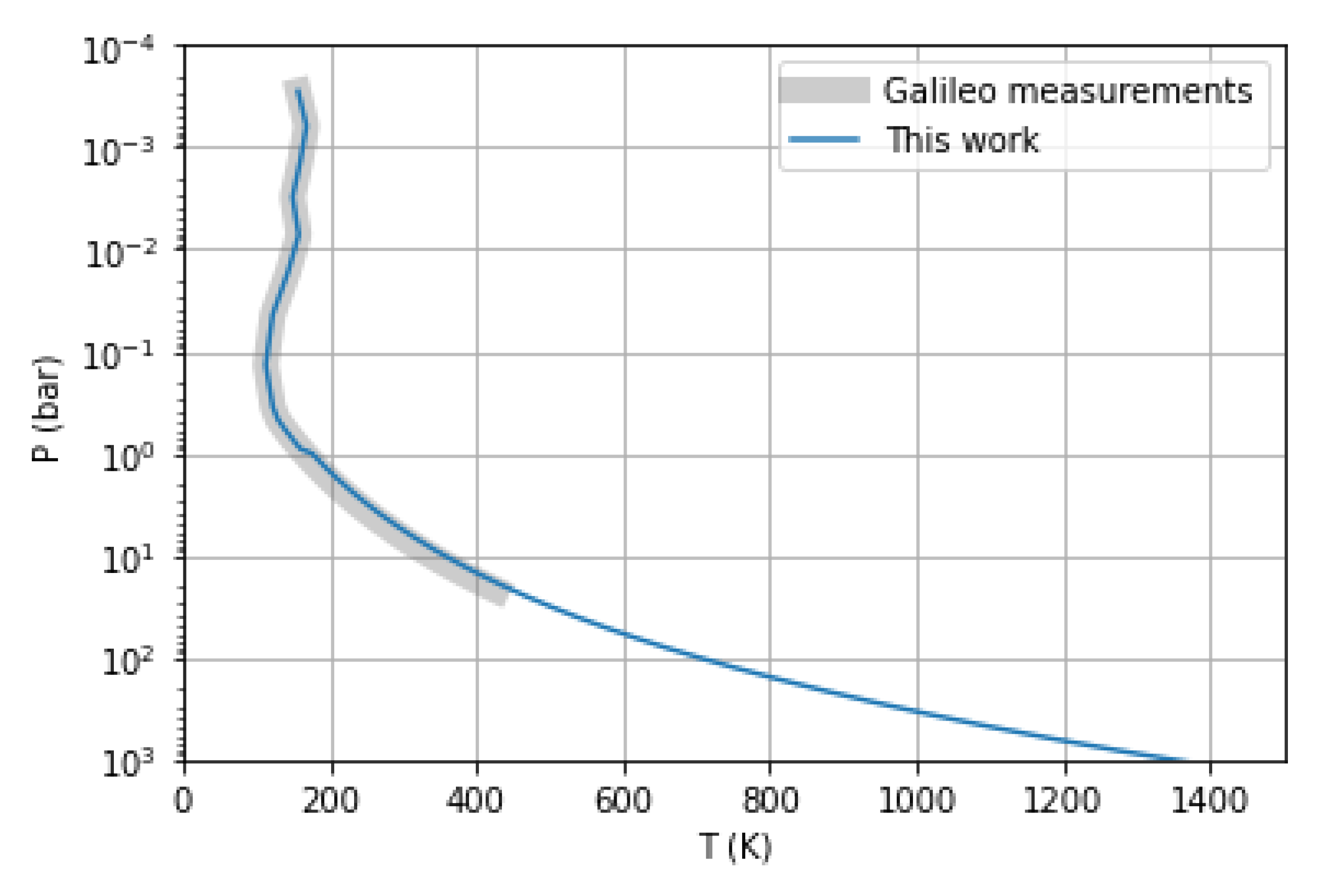
2.2. Thermal Profile
For the temperature profile, we use an adiabat that extends from the in situ Galileo measurements to the deep interior of the planet calculated by Miguel et al. (2022) [26] using the interior and evolution code CEPAM (Guillot and Morel (1995) [27]). These calculations correspond to one of the solutions to Jupiter’s internal structure that fits the observations on radius of the planet, gravitational harmonics and helium abundance by the Galileo probe, also considering the latest constraints on Jupiter’s differential rotation [28,29].
This profile and the Galileo measurements can be seen in Figure 1. We note that a reassessment of the Voyager Radio Occultation Measurements has been recently performed by Gupta et al. (2022) [30], which led to a higher temperature at 1 bar of 170.3 ± 3.8 K, when compared with the Galileo Probe values of 166.1 ± 0.8 K. This leads to an increase in the temperature of a few degrees. While this increase in temperature at 1 bar is extremely important for interior model calculations [26], our sensitivity study showed that it does not significantly affect the results of the chemical abundances at larger pressures. In this sensitivity study, we compared the location of reference points along chemical model lines using seven temperature–pressure profiles, each shifted in increments of 2 K at the interface of Galileo data to the model extension, and saw a negligible variation of the location of these reference points.
Figure 1.
The temperature–pressure profile used in this work. The grey shaded area denotes data from the Galileo entry probe.
2.3. Elemental Abundances
In this work, we assume that there is a strong vertical mixing that brings the species from the deep atmosphere (where they are in chemical equilibrium) to lower pressures where they are observed. While there are disequilibrium processes that might interfere [31], the analysis and significance of those in determining the bulk elemental abundance of the different species is an open question and out of the scope of this paper, whose focus is on the study of condensation and chemistry at higher pressures.
Table 1 gives a brief overview of the development of our knowledge on the enrichment of different species before and after Galileo and Juno. Since HO, NH, CH and HS are the dominant carriers of oxygen, nitrogen, carbon and sulphur, respectively, their enrichments can be taken to be constraints for the elemental abundances of those species. These values are compared against solar hydrogen abundance, as given by Anders and Grevesse (1989) [32] for the Galileo results (sulphur and carbon) and from Asplund et al. (2009) [33] for the Juno results (nitrogen and oxygen).
For the other metals, we used an enrichment factor of 2.3 as compared with solar values taken from Asplund et al. (2009). The list of elemental abundances can be found in Appendix A. It may be noted that elements, such as bromine, boron and iodine, are missing; this is due to their absence from the GGchem dataset at the time of this research.
We used Li et al. (2020) [6] for the Juno measurements of the water enrichment, E. This is a historically interesting value, since the in situ measurements of the Galileo entry probe were done in a 5 m ’hot-spot’, which is water-deprived [34]. Therefore, the values for E differ greatly between the two probes.
In addition to modelling the gas and condensate chemistry, we also want to investigate the effect of varying the water enrichment on our models, specifically the influence of the phyllosilicates. For the analysis of the influence of the water enrichment on our models, we used the minimal value adopted by Lodders et al. (2004) [35], E = 0.47, and the maximal value reported is E = 10, taken from the Shoemaker–Levy 9 impacts [36] (both values are compared with solar values).
Table 1.
Abundances of the dominant carriers of O, N, C and S in Jupiter’s atmosphere. The measurements are given as enrichment factors with respect to solar H. * Galileo results (1998, updated measurements in 2004) were taken with the GPMS, characteristically in a region now known to be anomalously dry (i.e., a water-deprived 5 m ’hotspot’). ** Juno results (2020) taken with the MWR instrument.
| Molecule (g) | Galileo (1998) [37] * | Galileo (2004) [38] * | Juno (2020) [6] ** |
|---|---|---|---|
| HO | ≤0.033 ± 0.015 | 0.289 ± 0.096 | 2.7 |
| NH | ≤10 | 2.96 ± 1.13 | 2.76 |
| CH | 2.9 | 3.27 ± 0.78 | - |
| HS | 2.5 | 2.75 ± 0.66 | - |
2.4. Condensation Data
Another parameter of high importance in the computation of our models is the included thermodynamic data of the condensed species. The condensates used are listed in Appendix B. We used 251 condensed species in our calculations, including phyllosilicates. These are silicate minerals, such as micas, chlorite talc and clay minerals, that are found to be stable at below 500–700 K [22] in solar-like composition gasses in phase equilibrium. Phyllosilicates interfere with the stability of liquid water and are furthermore of vital importance at lower temperatures as they can remove water from the gas phase [39].
The thermochemical data GGchem uses is taken from NIST-JANAF (1998) [40], which takes condensed thermochemical data from the geophysical SUPCRTBL database [41,42]. We note that iodine and bromine are altogether missing from the dataset used in this research, since the data available to GGchem is currently not complete—particularly for the condensate phase.
Fegley and Lodders (1994) model the most abundant bromine species, HBr, at around 10 mixing ratio, and the most abundant iodine species, HI, at around 10 mole fraction. Below these mole fractions, our models are influenced, since the species we model are not depleted according to available bromine and iodine abundances. Organic molecules, such as CHOH and CH, are not incorporated in the GGchem database for the same reasons. Other species that are similarly not available include SiO, HS, HS, NaS, KS and CH.
3. Results
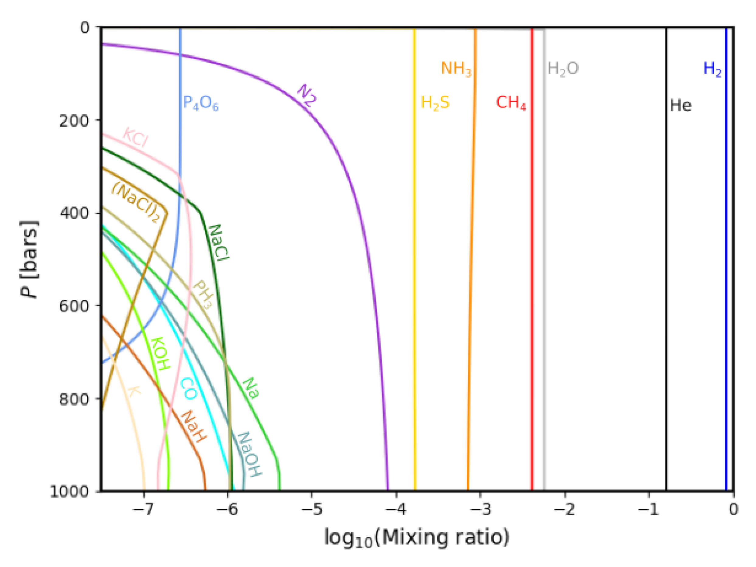
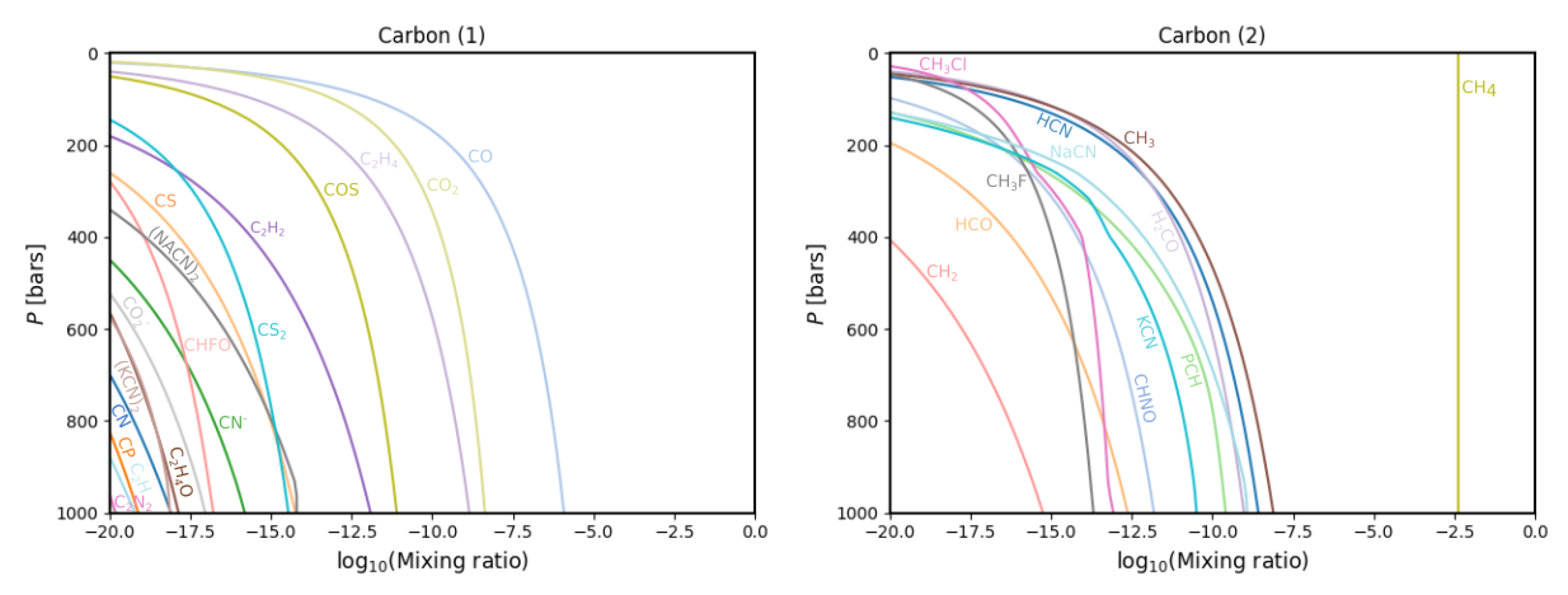
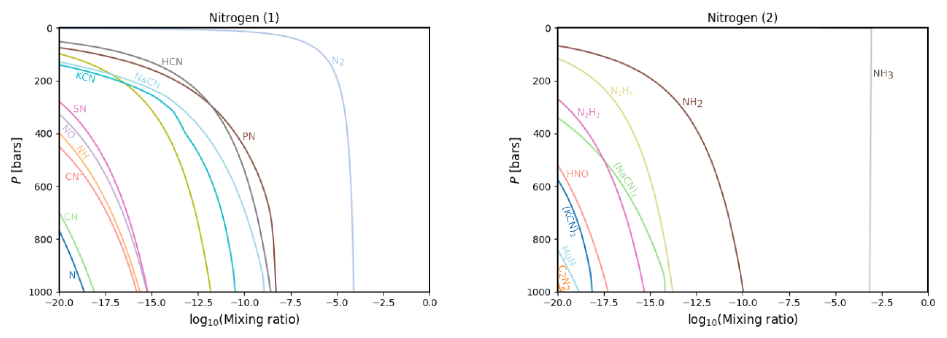
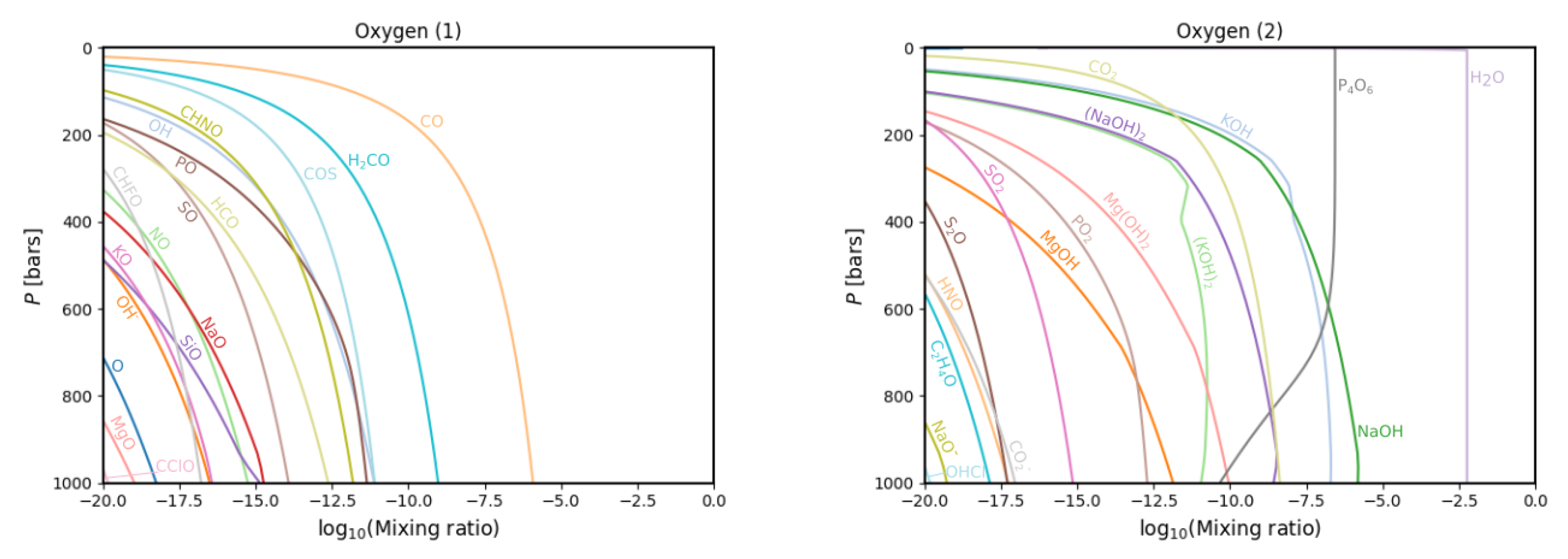
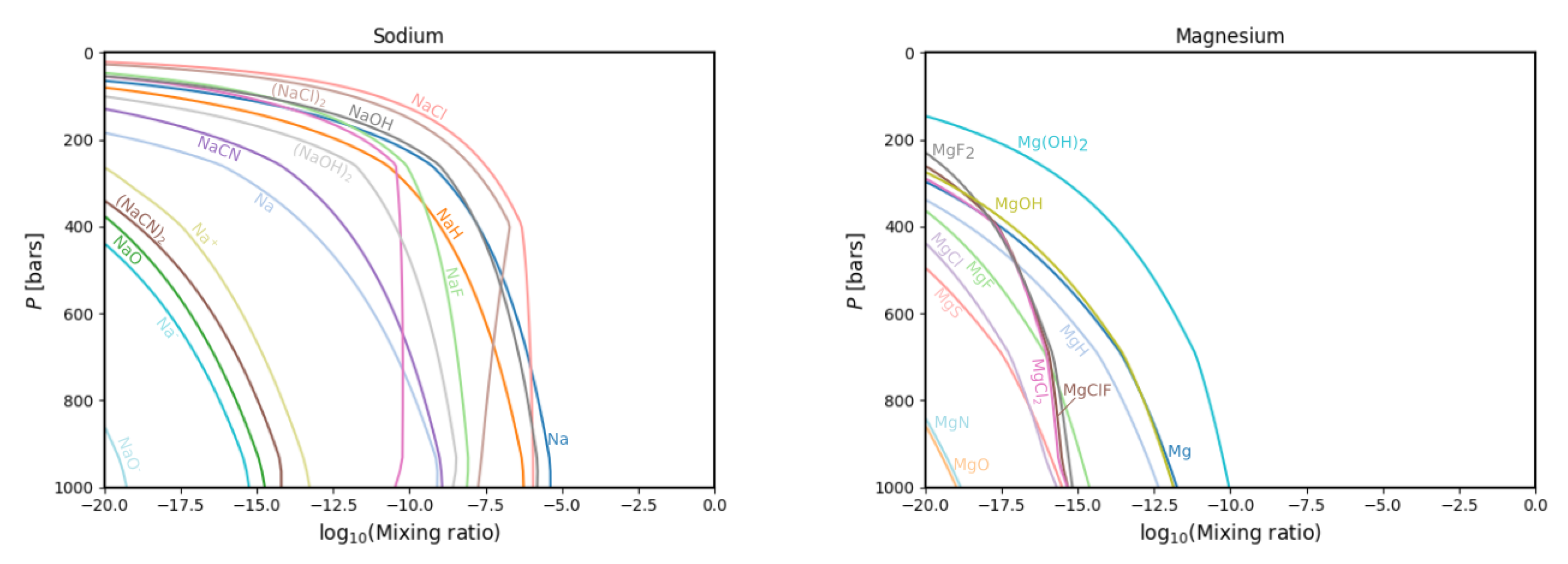
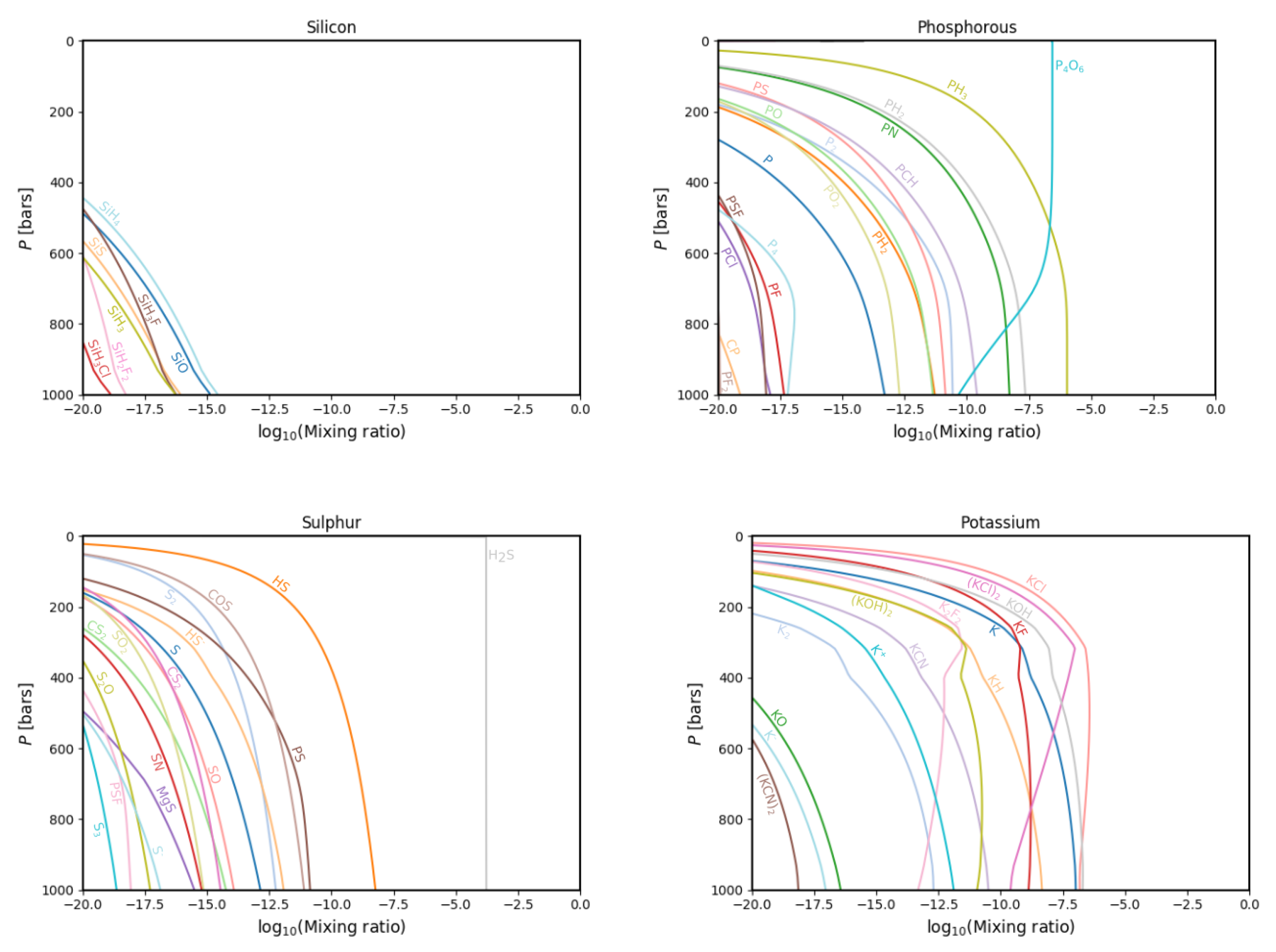
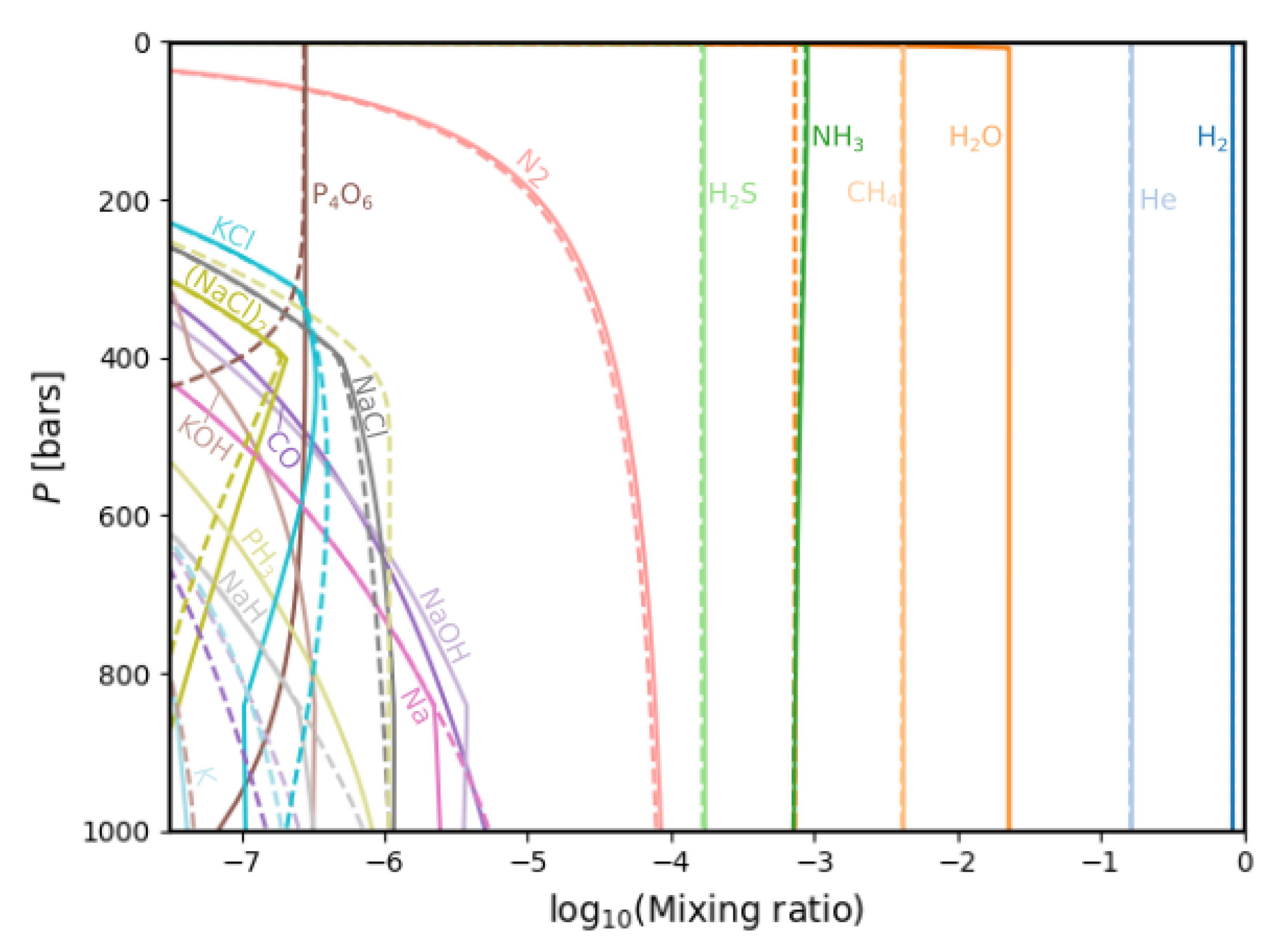
3.1. Gas Phase Chemistry
In addition to the background gases H and He, we are mainly interested in the elements C, N, O, Na, Mg, Si, P, S, Cl and K, being the next most abundant on Jupiter. A complete list of the elements used in our calculations is given in Appendix A.Their gas phase equilibrium chemistries are plotted against the pressure inverted on the vertical axes. To parametrize the altitude, down to 1000 bars, or roughly 1350 K, see Figure 2.
Figure 2.
The most abundant equilibrium gas phase compounds in the Jovian (deep) atmosphere.
In our atmospheric calculations with GGchem, we assume Jupiter’s atmosphere to be sufficiently well-described as an ideal gas. However, for pressures beyond ∼1000 bars, this becomes less accurate [43], and therefore we limit our models to that threshold. The logarithmic mixing ratios of the species, as compared to the total molar content, are given on the horizontal axes
Figure 2 gives an overview of the most abundant species, down to a mixing ratio of 10. In addition to H and He (the most dominant species) the most abundant are HO, CH and NH, which are the main carriers of O, C and N in this environment of cold temperatures and high H abundance. HS, the main carrier of S, follows, at all pressures, and N takes the place as the main carrier of nitrogen when the temperature increases at higher pressures.
At lower mixing ratios, species bearing potassium, sodium, phosphorous and chlorine are present. The abundance of the most abundant species, H, He, HO, CH, NH and HS, does not seem to vary with pressure. However, this variation does exist; however, because these species are =very abundant (they are the dominant carriers of S, N and C, respectively), these variations are incredibly minute and cannot be seen on a logarithmic scale. For instance, NH decreases in abundance with altitude, from 10 mixing ratio at the minimal pressure value to 10 mixing ratio at 1000 bars, due to depletion into the condensate phase; however, the condensate abundance and gas phase abundance are apart in two degrees of magnitude.
3.2. Comparisons with Previous Calculations
Figure 3, Figure 4, Figure 5, Figure 6 and Figure 7 give the complete collection of chemistries for the aforementioned elements, of which Figure 2 is only a selection. Comparing our results with those by Fegley and Lodders (1994), it is clear that the NH, N and HO mixing ratios are higher, which is consistent with the increased elemental enrichments of oxygen and nitrogen from the new Juno measurements. The same holds for CH and HS but from the Galileo measurements postdating those calculations.
Figure 3.
Gas phase chemistry for all carbon-bearing species that reach a peak mixing mixing ratio at some point in the atmosphere of more than a 10 mixing ratio. The species are split into two panels for clarity.
Figure 4.
The same as in Figure 3 but for the nitrogen gas phase chemistry.
Figure 5.
The same as in Figure 3 but for the oxygen gas phase chemistry.
Figure 6.
The same as in Figure 3 but for the sodium (left) and magnesium (right) gas phase chemistries.
Figure 7.
The same as in Figure 3 but for the silicon (top left), phorphorous (top right), sulphur (bottom left) and potassium (bottom right) gas phase chemistries.
The exact factors of change in the mixing ratio of these species with respect to Fegley and Lodders (1994) are as follows. Compared at 1000 bars, our measured NH mixing ratio is a factor 1.55 higher than Fegley and Lodders’ value. N increased by a factor of 5.89, HO by a factor of 1.78, CH by a factor of 2.82 and HS by a factor of 2.69. These increases are due to the new and increased elemental abundances taken from the Galileo and Juno data, since Fegley and Lodders assumed an enrichment factor of 2.3 for carbon and heavier atoms, and we used the most recent available enrichment factors as seen in Table 1.
Generally, all oxygen-, nitrogen-, carbon- and sulphur-bearing species, particularly the relatively abundant ones, follow this pattern. The only oxygen-, nitrogen-, carbon- or sulphur-bearing species that is less abundant in our models compared with previous calculations is PO. However, it is only very slightly less abundant (by a factor of 1.44) but extends to the lowest pressure, whereas PO disappears from Fegley and Lodders’ model at around 30 bars of pressure. The effect of the increased enrichment of oxygen is, therefore, still noticeable in PO.
Of the other abundant molecules (i.e., those included in Figure 2), the following are more abundant in our models than in Fegley and Lodders: NaCl (by a factor 1.62), KCl (a factor of 1.55) and (NaCl) (a factor of 14.45). For the case of the two chlorine-bearing species, this increase can be explained by our calculations not resulting in condensed NaBO (s) at all and NaS (s) in vastly lower mixing ratios, therefore, depleting these gas phase species less.
The increase in gaseous KCl is caused in a similar way, since our condensate models do not include any potassium species. Finally, the species from Figure 2 that are less abundant in our models as compared with Fegley and Lodders are Na (by a factor of 1.41), PH (a factor of 1.41), NaH (a factor of 1.58) and K (a factor of 1.51). In the case of phosphorous, this is again likely due to condensate depletion because Fegley and Lodders’ models displayed condensed NHHPO (s), whereas ours did not. The cause of the decrease in abundance of the simple molecules Na, NaH and K is less evident but could be related to the condensate chemistry as well.
In addition to the new data used, an important source of discrepancy with previous calculations is the thermodynamic data and its availability. Many gas species are either present or absent simply because of their presence in the database available in GGchem. Our results differ from Fegley and Lodders mainly in terms of the used dataset and through the new enrichment factors for oxygen, nitrogen, carbon and sulphur. Our models, therefore, include new species or exclude species that were modelled before. This generally corresponds with the molecules’ presence in the databases, be it for Fegley and Lodders or the current research. Since the most abundant species are already discussed above, we will discuss the occurrence of the trace species below.
In the carbon gas chemistry (Figure 3), we find a large number of new species, the most abundant of which are CN, CHFO, CClO and the charged CN and CO. The first three were absent in Fegley and Lodders’ database, and the latter two were present in their database but did not arise in their plots, likely due to oxygen and nitrogen depleting to the more abundant species, which are further enriched in our models than they were in Fegley and Lodders.Furthermore, carbon species missing from these results are CHOH, CH and CH. The last is not part of the database used for this work; the other two do not arise in our calculations. This is also presumed to be caused by depletion to the more abundant, further enriched species.
The results for nitrogen are shown in Figure 4. Missing from these models as compared with prior calculations is CHNH, which was absent in our database. New species include (NaCN), NH, N and HNO. The first was indeed absent from Fegley and Lodders’ database; however, the latter three were present in it. It must therefore be concluded that their presence in our models is due to the enrichment of nitrogen and oxygen, which they carry.
The most important novelty in the oxygen chemistry modelled here (Figure 5) is the upward shift in abundance. This holds for the dominant species HO, CO and CO. This is due to the increased enrichment of oxygen taken from Juno data. Important to note as well is the lack of organic molecules, such as CHOH, CHCOOH and CHOOH, which are absent from the dataset we used.
In the case of sodium (Figure 6, left panel), we find Na, Na, NaO and (NaCN). All except (NaCN) were present in Fegley and Lodders’ dataset but not modelled. This could be due to their low abundance—particularly NaO.
In the magnesium gas chemistry (Figure 6, right panel) we find no new species, only a lack of previously modelled species, namely MgBr, MgI and Mg. The former two were not present in the database from GGchem, while Mg was. Since the molecule is only present at great depths in Fegley and Lodders’ model, its absence in our models can be explained by depletion to the condensate phase.
Similarly, no new silicon species are found (Figure 7, top left panel), while many are not resultant in our models that were present in Fegley and Lodders (1994) [18], namely SiHF, SiF, SiOF, SiI, SiBr, SiF, SiHCl, SiCl, SiOF, SiH, SiN, SiN, SiC, Si, SiTe, SiSe, SiO, and SiH.
Of these, all but SiCl, SiN and SiO were absent in the used database. That these three do not occur in our model can only partly be understood as depletion to the abundant, enriched nitrogen- and oxygen-carrying species. That a chlorine-carrying molecule, SiCl, is absent from our models is likely caused by the presence of a large number of chlorine-carrying condensate species, to which the chlorine is depleted at higher pressures.
A somewhat significant new phosphorous species (Figure 7, top right panel) is PSF. Consistent with the increase of elemental abundances of nitrogen, sulphur and oxygen, the models here presented show an increase in abundance of PN, PS and PO. In the case of sulphur (Figure 7, bottom left panel), newly found species are SO, S, S and HS. The last was not present in Fegley and Lodders’ dataset; however, the first three were. This can be due to the increased enrichment of sulphur in our models.
The potassium chemistry (Figure 7, bottom right panel) is updated slightly in comparison with previous models in terms of the addition of positively and negatively charged atomic potassium and (KCN), which were both not present in Fegley and Lodders’ dataset. Species that do not follow in our models are KBr, KI and KBr since we do not include bromine and iodine themselves in our dataset, KS and KS. These last two were indeed also not present in our dataset.
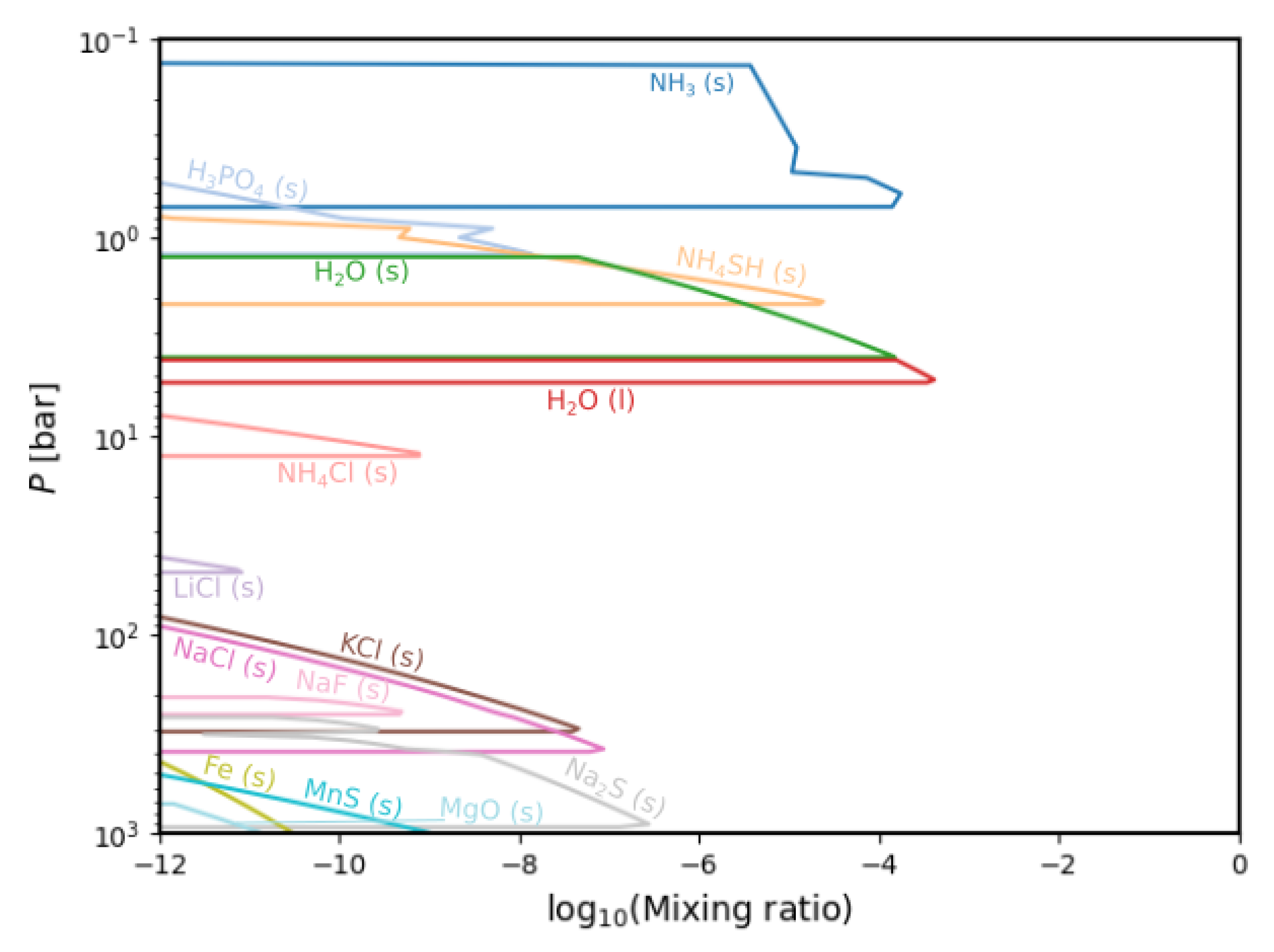
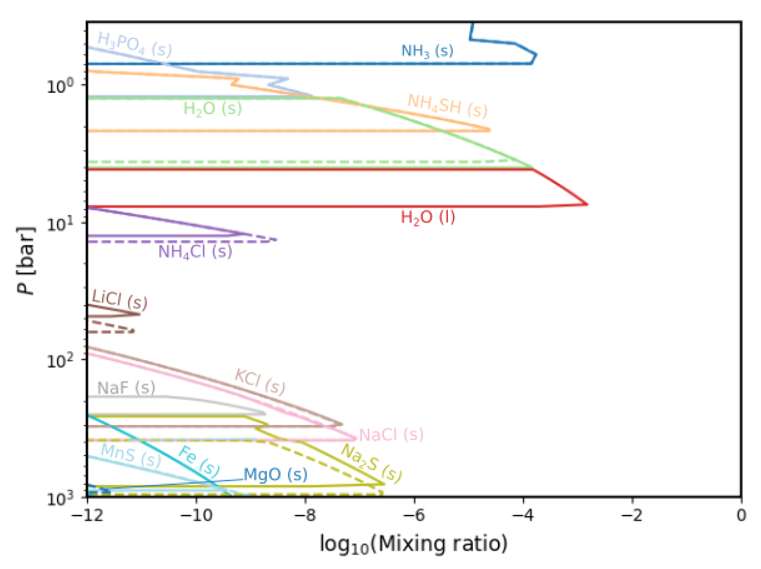
3.3. Condensation Chemistry
Figure 8 plots the species that condensed out of the gas phase into either the liquid or solid state. Table 2 shows their formation conditions.
Figure 8.
Condensation chemistry in the deep Jovian atmosphere. Species denoted [l] are liquids; the others are solids.
Table 2.
Condensate equilibrium species and the corresponding formation conditions.
The results for the condensation chemistry generally correspond with observations and prior models starting with NH (s), NHSH (s) and HO (s, l) clouds dominating the upper layer of the atmosphere. At this level, we also find HPO (s), which is remarkable since we do not find it as a gas species in our models, as is the case in Wang (2016) [12]. Nevertheless, we note that the model by [12] considers disequilibrium chemistry, and this might be the source of the main differences. Continuing in depth, our models show a chlorine-dominated region with several sodium species below that.
Comparing these models to Fegley and Lodders (1994) [18], we find significant changes. Most importantly, our calculations extend to temperatures of 100 K and include the condensation of NH (s) and HO (s), which were out of the scope of previous calculations that were made with temperatures as cold as 298.15 K.
We find several new species, namely HPO (s), LiCl (s), KCl (s), NaCl (s), NaF (s), MgO (s), Fe (s) and MnS (s). Notable as well are the condensates that we no do not find but were modelled by, for instance, Fegley and Lodders (1994) [18], namely NHHPO (s), KS (s), KBO (s), RbCl (s), NaBO, NHF (s), NHI (s), LiS (s), LiBO (s) and MgSiO (s, l). All except MgSiO (s, l) are absent in the used dataset. This molecule is calculated but arises below 1000 bars of pressure and is therefore not plotted.
4. Discussion
Figure 9 shows a comparison between the different gas chemistries found when considering different initial water abundances at low pressure in the atmosphere. We compare the case of E = 0.47 (in dashed lines) with the case of E = 10 (in solid lines). As seen in Figure 9, the mixing ratios of HO, CO, NaOH, NaCl, PO and (NaCl) decrease with increasing E. No significant changes are found for H, He, CH and NH. HS and N decrease only slightly. The species Na, PH, KCl and K increase in mixing ratio with a decreasing water enrichment.
Figure 9.
Comparison between the gas chemistry for minimal (dashed lines, E = 0.47) and maximal (solid lines, E = 10) HO enrichment values.
Figure 10 shows the condensation modelled chemistry for the two extremal water abundances. For E = 0.47, we find that HO (l) no longer condenses. Almost half of the number of species experiences a decrease in abundance with a decrease in water enrichment, namely HO (s), HO (l), NHCl, NaF, Fe, MnS and MnO. The liquid water does not condensate at all with the minimal water enrichment value. Several of these species also only condense at greater depths than before—primarily LiCl and Fe. Importantly, our results place a lower limit on the elemental abundance of water necessary for liquid water clouds to form.
Figure 10.
Comparison between the condensate chemistry for minimal (dashed lines, E = 0.47) and maximal (straight lines, E = 10) HO enrichment values.
5. Conclusions
In this research, we constructed models for the thermochemical equilibrium gas phase and condensate chemistry of the deep atmosphere of Jupiter. Our results show complete chemical profiles of gaseous species down to mixing ratios of 10 and condensate species down to mixing ratios of 10 for pressures up to 1000 bars. The primary incentive to do this study was the need for new calculations to estimate the deep atmospheric composition of Jupiter and cloud formation at pressures not available for remote sensing using, as input data, the abundances measured by the Galileo and Juno missions.
The thermochemical calculations were done for the nine most abundant elements following H and He, namely C, N, O, P, S, K, Na, Mg and Si. Our measurements used a deep thermal profile calculated by state-of-the-art interior structure models that fit the Juno gravitational constraints [26]. We also used new elemental abundances for C, N, O and S based on measurements of their dominant molecular carriers (CH, NH, HO and HS, respectively) from both Galileo and Juno.
Several new gas phase and condensed species were found. The new, previously unreported gas species are CN, CHFO, CClO, CN, CO, (NaCN), NH, N, HNO, Na, Na, NaO, (NaCN), PSF, SO, S−, S and HS. The condensation chemistry calculations presented here replicate observations from the upper atmosphere closely and are generally also in line with calculations of deeper chemistry, though not reaching far enough depths to include mineral species. Newly found species are NH (s), HO (s), HPO (s), LiCl (s), KCl (s), NaCl (s), NaF (s), MgO (s), Fe (s) and MnS (s).
The effect of the increased elemental abundances can be clearly seen, as the most abundant gas phase species carrying C, N, O and S each increase by several factors as compared with previous investigations: NH increased by 1.55, N by 5.89, HO by 1.78, CH by 2.82 and HS by 2.69. Furthermore, we investigated the influence of the water enrichment on our models by comparing two extreme values taken from the literature, namely E = 047 and E = 10. We found that the elemental enrichment of oxygen required for water clouds to form was higher than expected.
Our results can serve as a reference for future calculations of opacities and interior models and are crucial for understanding the abundances of important elements, such as HO, at great depths to inform planet formation studies.
Author Contributions
Conceptualization, Y.M.; methodology, Y.M. and F.R.; software, P.W., C.H., O.H. and F.R.; validation, Y.M.; formal analysis, F.R.; investigation, F.R., M.Z. and A.L.; resources, Y.M.; data curation, F.R.; writing—original draft preparation, F.R.; writing—review and editing, Y.M., P.W., C.H. and O.H.; visualization, F.R.; supervision, Y.M., M.Z. and A.L.; project administration, Y.M. This research received no funding. All authors have read and agreed to the published version of the manuscript.
Funding
This research received no external funding.
Data Availability Statement
Not applicable.
Conflicts of Interest
The authors declare no conflict of interest.
Appendix A. Elemental Abundances Used in the Calculations
| H | 12.0 |
| He | 10.98 |
| Li | 1.451727836017593 |
| C | 9.386275588677877 |
| N | 8.712636918082811 |
| O | 9.56309160017658 |
| F | 4.961727836017593 |
| Na | 6.641727836017593 |
| Mg | 8.001727836017594 |
| Al | 6.851727836017593 |
| Si | 7.911727836017593 |
| P | 5.811727836017593 |
| S | 8.001060529847855 |
| Cl | 5.901727836017593 |
| K | 5.431727836017593 |
| Ca | 6.741727836017593 |
| Ti | 5.351727836017593 |
| V | 4.331727836017593 |
| Cr | 6.041727836017593 |
| Mn | 5.831727836017593 |
| Fe | 7.901727836017593 |
| Co | 5.391727836017593 |
| Ni | 6.621727836017593 |
| Zr | 2.9817278360175923 |
| W | 1.2517278360175919 |
Appendix B. List of Condensed Species Considered in the Calculations
| Al2O3[s] | CORUNDUM(alpha) |
| Al2O3[l] | CORUNDUM(liquid) |
| MgAl2O4[s] | SPINEL |
| MgAl2O4[l] | SPINEL(liquid) |
| TiO2[s] | RUTILE |
| TiO2[l] | RUTILE(liquid) |
| Ti4O7[s] | TITANIUM-OXIDE |
| Ti4O7[l] | TITANIUM-OXIDE(liquid) |
| Mg2SiO4[s] | FOSTERITE |
| Mg2SiO4[l] | FOSTERITE(liquid) |
| MgSiO3[s] | ENSTATITE |
| MgSiO3[l] | ENSTATITE(liquid) |
| Fe[s] | IRON(alpha-delta) |
| Fe[l] | IRON(liquid) |
| Fe2SiO4[s] | FAYALITE |
| FeS[s] | TROILITE |
| FeS[l] | TROILITE(liquid) |
| MgTi2O5[s] | MG-DITITANATE |
| MgTi2O5[l] | MG-DITITANATE(liquid) |
| C[s] | GRAPHITE |
| TiC[s] | TITANIUM-CARBIDE |
| TiC[l] | TITANIUM-CARBIDE(liquid) |
| SiC[s] | SILICON-CARBIDE(alpha) |
| SiO[s] | SILICON-MONOXIDE |
| SiO2[s] | QUARTZ |
| SiO2[l] | QUARTZ(liquid) |
| Zr[s] | ZIRCONIUM(beta) |
| Zr[l] | ZIRCONIUM(liquid) |
| ZrO2[s] | BADDELEYITE |
| ZrO2[l] | BADDELEYITE(liquid) |
| ZrSiO4[s] | ZR-SILICATE |
| W[s] | TUNGSTEN |
| W[l] | TUNGSTEN(liquid) |
| WO3[s] | W-TRIOXIDE |
| WO3[l] | W-TRIOXIDE(liquid) |
| MgO[s] | PERICLASE |
| MgO[l] | PERICLASE(liquid) |
| FeO[s] | FERROPERICLASE |
| FeO[l] | FERROPERICLASE(liquid) |
| Na2SiO3[s] | NA-METASILICATE |
| Na2SiO3[l] | NA-METASILICATE(liquid) |
| H2O[s] | WATER-ICE |
| H2O[l] | WATER(liquid) |
| NH3[s] | AMONIA(liquid/solid) |
| CH4[s] | METHANE(liquid/solid) |
| CO[s] | C-MONOXIDE(liquid/solid) |
| CO2[s] | C-DIOXIDE(liquid/solid) |
| H2SO4[s] | SULPHURIC-ACID |
| H2SO4[l] | SULPHURIC-ACID(liquid) |
| Na[s] | SODIUM |
| Na[l] | SODIUM(liquid) |
| NaCl[s] | HALITE |
| NaCl[l] | HALITE(liquid) |
| KCl[s] | SYLVITE |
| KCl[l] | SYLVITE(liquid) |
| S[s] | SULPHUR |
| S[l] | SULPHUR(liquid) |
| MgS[s] | MG-SULPHIDE |
| LiCl[s] | LI-CHLORIDE |
| LiCl[l] | LI-CHLORIDE(liquid) |
| AlCl3[s] | AL-TRICHLORIDE |
| AlCl3[l] | AL-TRICHLORIDE(liquid) |
| CaO[s] | LIME |
| CaO[l] | LIME(liquid) |
| CaCl2[s] | CA-DICHLORIDE |
| CaCl2[l] | CA-DICHLORIDE(liquid) |
| LiH[s] | LI-HYDRIDE |
| LiH[l] | LI-HYDRIDE(liquid) |
| MgTiO3[s] | GEIKIELITE |
| MgTiO3[l] | GEIKIELITE(liquid) |
| K2SiO3[s] | K-SILICATE |
| K2SiO3[l] | K-SILICATE(liquid) |
| Ti[s] | TITANIUM(beta) |
| Ti[l] | TITANIUM(liquid) |
| TiO[s] | TI-MONOXIDE(beta) |
| TiO[l] | TI-MONOXIDE(liquid) |
| LiOH[s] | LI-HYDROXIDE |
| LiOH[l] | LI-HYDROXIDE(liquid) |
| VO[s] | V-MONOXIDE |
| VO[l] | V-MONOXIDE(liquid) |
| V2O3[s] | KARELIANITE |
| V2O4[s] | PARAMONTROSEITE |
| V2O5[s] | SHCHERBINAITE |
| CaS[s] | CALCIUM-SULFIDE |
| FeS2[s] | PYRITE |
| Na2S[s] | NA-SULFIDE |
| Mn[s] | MANGANESE(alpha-delta) |
| Mn[l] | MANGANESE(liquid) |
| MnS[s] | ALABANDITE |
| Ni[s] | NICKEL |
| Ni[l] | NICKEL(liquid) |
| Ni3S2[s] | HEAZLEWOODITE |
| Ni3S2[l] | HEAZLEWOODITE(liquid) |
| Cr[s] | CHROMIUM |
| Cr[l] | CHROMIUM(liquid) |
| CrN[s] | CARLSBERGITE |
| CaSiO3[s] | WOLLASTONITE |
| CaTiO3[s] | PEROVSKITE |
| NiS[s] | MILLERITE |
| NiS2[s] | VAESITE |
| Ca2Al2SiO7[s] | GEHLENITE |
| Ca3Al2Si3O12[s] | GROSSULAR |
| Ca2SiO4[s] | LARNITE |
| CaAl2SiO6[s] | Ca-TSCHERMAKS |
| Ca3Si2O7[s] | RANKINITE |
| Ca5P3O12F[s] | FLUORAPATITE |
| Ca3MgSi2O8[s] | MERWINITE |
| CaAl2Si2O8[s] | ANORTHITE |
| CaTiSiO5[s] | SPHENE |
| Ca2MgSi2O7[s] | AKERMANITE |
| Al2SiO5[s] | KYANITE |
| CaMgSiO4[s] | MONTICELLITE |
| CaMgSi2O6[s] | DIOPSIDE |
| MgAl2SiO6[s] | Mg-TSCHERMAKS |
| KMg3AlSi3O10F2[s] | FLUORPHLOGOPITE |
| Mg3Al2Si3O12[s] | PYROPE |
| Ca2Al3Si3O13H[s] | CLINOZOISITE |
| CaSi2O5[s] | CaSi-TITANITE |
| Ca5Si2CO11[s] | SPURRITE |
| KAlSi3O8[s] | MICROCLINE |
| Ca5P3O13H[s] | HYDROXYAPATITE |
| KAlSiO4[s] | KALSILITE |
| KAlSi2O6[s] | LEUCITE |
| NaAlSi3O8[s] | ALBITE |
| NaAlSi2O6[s] | JADEITE |
| NaAlSiO4[s] | NEPHELINE |
| Ca2MnAl2Si3O13H[s] | PIEMONTITE(ORDERED) |
| CaAl4Si2O12H2[s] | MARGARITE |
| Ca2Al2Si3O12H2[s] | PREHNITE |
| Ca2FeAl2Si3O13H[s] | EPIDOTE(ORDERED) |
| Ca5Si2C2O13[s] | TILLEYITE |
| Ca3Fe2Si3O12[s] | ANDRADITE |
| KMg2Al3Si2O12H2[s] | EASTONITE |
| Mn3Al2Si3O12[s] | SPESSARTIN |
| CaFeSi2O6[s] | HEDENBERGITE |
| Mg3Cr2Si3O12[s] | KNORRINGITE |
| K2Si4O9[s] | Si-WADEITE |
| Mg2Al2Si3O12H2[s] | TSCHERMAK-TALC |
| KAl3Si3O12H2[s] | MUSCOVITE |
| KMg3AlSi3O12H2[s] | PHLOGOPITE |
| NaAl3Si3O12H2[s] | PARAGONITE |
| AlSi2O6H[s] | PYROPHYLLITE |
| NaMg3AlSi3O12H2[s] | SODAPHLOGOPITE |
| FeAl2O4[s] | HERCYNITE |
| Mg3Si4O12H2[s] | TALC |
| KMgAlSi4O12H2[s] | CELADONITE |
| NaCrSi2O6[s] | KOSMOCHLOR |
| Ca2FeAlSi3O12H2[s] | FERRI-PREHNITE |
| MnTiO3[s] | PYROPHANITE |
| Ca2Fe2AlSi3O13H[s] | Fe-EPIDOTE |
| MgAl2SiO7H2[s] | Mg-CHLORITOID |
| MnSiO3[s] | PYROXMANGITE |
| CaAl2Si4O14H4[s] | WAIRAKITE |
| KAlSi3O9H2[s] | K-CYMRITE |
| Fe3Al2Si3O12[s] | ALMANDINE |
| Al2SiO6H2[s] | HYDROXY-TOPAZ |
| KFeAlSi4O12H2[s] | FERROCELADONITE |
| NaFeSi2O6[s] | ACMITE |
| MnAl2SiO7H2[s] | Mn-CHLORITOID |
| NaAlSi2O7H2[s] | ANALCITE |
| CaAl2Si2O10H4[s] | LAWSONITE |
| MgCr2O4[s] | PICROCHROMITE |
| Mn2SiO4[s] | TEPHROITE |
| KMn3AlSi3O12H2[s] | Mn-BIOTITE |
| MgAl2Si2O10H4[s] | MAGNESIOCARPHOLITE |
| FeTiO3[s] | ILMENITE |
| AlO2H[s] | DIASPORE |
| FeAl2SiO7H2[s] | Fe-CHLORITOID |
| Mg7Si2O14H6[s] | PHASEA |
| CaCO3[s] | CALCITE |
| Mg3Si2O9H4[s] | LIZARDITE |
| Al2Si2O9H4[s] | KAOLINITE |
| FeSiO3[s] | FERROSILITE |
| CaSO4[s] | ANHYDRITE |
| KFe3AlSi3O12H2[s] | ANNITE |
| CaMgC2O6[s] | DOLOMITE |
| CaAl2Si4O16H8[s] | LAUMONTITE |
| FeAl2Si2O10H4[s] | FERROCARPHOLITE |
| Fe3Si4O12H2[s] | MINNESOTAITE |
| Cr2O3[s] | ESKOLAITE |
| MgCO3[s] | MAGNESITE |
| Fe2TiO4[s] | ULVOSPINEL |
| MgFe2O4[s] | MAGNESIOFERRITE |
| CaFeC2O6[s] | ANKERITE |
| MnO[s] | MANGANOSITE |
| NaAlCO5H2[s] | DAWSONITE |
| Mn2O3[s] | BIXBYITE |
| MgO2H2[s] | BRUCITE |
| Fe3Si2O9H4[s] | GREENALITE |
| MnCO3[s] | RHODOCHROSITE |
| Fe2O3[s] | HEMATITE |
| Fe3O4[s] | MAGNETITE |
| FeCO3[s] | SIDERITE |
| FeO2H[s] | GOETHITE |
| NiO[s] | NICKEL |
| CuO[s] | TENORITE |
| Cu2O[s] | CUPRITE |
| Cu[s] | COPPER |
| NH4Cl[s] | AMMONIUM-CHLORIDE |
| NH4SH[s] | AMMONIUM-HYDROSULFIDE |
| H2S[s] | HYDROGEN-SULFIDE(liquid/solid) |
| S2[s] | Disulfer(liquid/solid) |
| S8[s] | Octasulfur(liquid/solid) |
| P[s] | PHOSPHORUS_WHITE |
| P[l] | PHOSPHORUS(liquid) |
| P4O10[s] | PHOSPHORUS-OXIDE |
| P4S3[s] | PHOSPHORUS-SULFIDE |
| P4S3[l] | PHOSPHORUS-SULFIDE(liquid) |
| Zn[s] | ZINC |
| Zn[l] | ZINC(liquid) |
| ZnSO4[s] | ZINC-SULFATE |
| ZnS[s] | SPHALERITE/WURTZITE |
| H3PO4[s] | PHOSPHORIC-ACID |
| H3PO4[l] | PHOSPHORIC-ACID |
| Mg3P2O8[s] | MAGNESIUM-PHOSPHATE |
| P3N5[s] | PHOSPHORUS-NITRIDE |
| AlF3[s] | ALUMINUM-FLUORIDE |
| CaF2[s] | FLUORITE |
| KF[s] | POTASSIUM-FLUORIDE |
| NaF[s] | SODIUM-FLUORIDE |
| FeF2[s] | IRON-FLUORIDE |
| MgF2[s] | MAGNESIUM-FLUORIDE |
| MgF2[l] | MAGNESIUM-FLUORIDE |
| HF2K[s] | POTASSIUM-BIFLUORIDE |
| AlF6Na3[s] | CRYOLITE |
| Li2SiO3[s] | LI-SILICATE |
| Li2SiO3[l] | LI-SILICATE |
| Li2Si2O5[s] | LI-SILICATE |
| Li2Si2O5[l] | LI-SILICATE |
| Li2TiO3[s] | LI-TITANATE |
| Li2TiO3[l] | LI-TITANATE |
| Co[s] | COBALT |
| Co[l] | COBALT(liquid) |
| CoO[s] | COBALT-MONOOXIDE |
| Ti3O5[s] | TITANIUM-OXIDE |
| Ti3O5[l] | TITANIUM-OXIDE(liquid) |
| Mg2TiO4[s] | QANDILIT |
| Mg2TiO4[l] | QANDILIT(liquid) |
| TiN[s] | TITANIUM-NITRIDE |
| TiN[l] | TITANIUM-NITRIDE(liquid) |
| TiF4[s] | TITANIUM-TETRAFLUORIDE |
| TiF3[s] | TITANIUM-TRIFLUORIDE |
| TiCl4[s] | TITANIUM-TETRACHLORIDE |
| TiCl4[l] | TITANIUM-TETRACHLORIDE(liquid) |
| TiCl3[s] | TITANIUM-TRICHLORIDE |
| TiCl2[s] | TITANIUM-DICHLORIDE |
| TiH2[s] | TITANIUM-HYDRIDE |
| FeCl2[s] | IRON-DICHLORIDE |
| FeCl2[l] | IRON-DICHLORIDE(liquid) |
| FeCl3[s] | IRON-TRICHLORIDE |
| FeCl3[l] | IRON-TRICHLORIDE(liquid) |
| AlO3H3[s] | GIBBSITE |
| Fe3O4[l] | MAGNETITE(liquid) |
References
- Guillot, T.; Cheng, L.; Scott, J.; Brown, S.; Ingersoll, A.; Janssen, M.; Levin, S.; Lunine, J.; Orton, G.; Steffes, P.; et al. Storms and the Depletion of Ammonia in Jupiter: II. Explaining the Juno Observations. J. Geophys. Sci. Planets 2020, 125, e2020JE006404. [Google Scholar] [CrossRef]
- Guillot, T.; Cheng, L.; Scott, J.; Brown, S.; Ingersoll, A.; Janssen, M.; Levin, S.; Lunine, J.; Orton, G.; Steffes, P.; et al. Storms and the Depletion of Ammonia in Jupiter: I. Microphysics of ‘Mushballs’. J. Geophys. Sci. Planets 2020, 125, e2020JE006403. [Google Scholar] [CrossRef]
- Mousis, O.; Marboeuf, U.; Lunine, J.I.; Alibert, Y.; Fletcher, L.N.; Orton, G.S.; Pauzat, F.; Ellinger, Y. Determination of the Minimum Masses of Heavy Elements in the Envelopes of Jupiter and Saturn. Astrophys. J. 2009, 696, 1348–1354. [Google Scholar] [CrossRef]
- Bolton, S.J.; Adriani, A.; Adumitroaie, V.; Allison, M.; Anderson, J.; Atreya, S.; Bloxham, J.; Brown, S.; Connerney, J.E.P.; DeJong, E.; et al. Jupiter’s interior and deep atmosphere: The initial pole-to-pole passes with the Juno spacecraft. Science 2017, 356, 821–825. [Google Scholar] [CrossRef]
- Grassi, D.; Adriani, A.; Mura, A.; Atreya, S.K.; Fletcher, L.N.; Lunine, J.I.; Orton, G.S.; Bolton, S.; Plainaki, C.; Sindoni, G.; et al. On the Spatial Distribution of Minor Species in Jupiter’s Troposphere as Inferred From Juno JIRAM Data. J. Geophys. Res. (Planets) 2020, 125, e06206. [Google Scholar] [CrossRef]
- Li, C.; Ingersoll, A.; Bolton, S.; Levin, S.; Janssen, M.; Atreya, S.; Lunine, J.; Steffes, P.; Brown, S.; Guillot, T.; et al. The water abundance in Jupiter’s equatorial zone. Nat. Astron. 2020, 4, 609–616. [Google Scholar] [CrossRef]
- Visscher, C. Mapping Jupiter’s Mischief. J. Geophys. Res. Planets 2020, 125, e2020JE006526. [Google Scholar] [CrossRef]
- Li, C.; Ingersoll, A.; Janssen, M.; Levin, S.; Bolton, S.; Adumitroaie, V.; Allison, M.; Arballo, J.; Bellotti, A.; Brown, S.; et al. The distribution of ammonia on Jupiter from a preliminary inversion of Juno microwave radiometer data. Geophys. Res. Lett. 2007, 44, 5317–5325. [Google Scholar] [CrossRef]
- Helled, R.; Lunine, J. Measuring Jupiter’s water abundance by Juno: The link between interior and formation models. Mon. Not. R. Astron. Soc. 2014, 441, 2273–2279. [Google Scholar] [CrossRef]
- Bosman, A.D.; Cridland, A.J.; Miguel, Y. Jupiter formed as a pebble pile around the N2 ice line. Astron. Astrophys. 2019, 632, L11. [Google Scholar] [CrossRef]
- Öberg, K.I.; Wordsworth, R. Jupiter’s Composition Suggests its Core Assembled Exterior to the N2 Snowline. Astron. J. 2019, 158, 194. [Google Scholar] [CrossRef]
- Wang, D.; Lunine, J.; Mousis, O. Modeling the disequilibrium species for Jupiter and Saturn: Implications for Juno and Saturn entry probe. Icarus 2016, 276, 21–38. [Google Scholar] [CrossRef]
- Zhang, Z.; Adumitroaie, V.; Allison, M.; Arballo, J.; Atreya, S.; Bjoraker, G.; Bolton, S.; Brown, S.; Fletcher, L.; Guillot, T.; et al. Residual Study: Testing Jupiter Atmosphere Models Against Juno MWR Observations. Earth Space Sci. 2020, 7, e2020EA001229. [Google Scholar] [CrossRef]
- Freedman, R.; Lustig-Yeager, J.; Fortney, J.; Lupu, R.; Marley, M.; Lodders, K. Gaseous Mean Opacities for Giant Planet and Ultracool Dwarf Atmospheres over a Range of Metallicities and Temperatures. Astrophys. J. Suppl. Ser. 2014, 214, 25. [Google Scholar] [CrossRef]
- Guillot, T.; Gautier, D.; Chabrier, G.; Mosser, B. Are the Giant Planets Fully Convective? Icarus 1994, 112, 337–353. [Google Scholar] [CrossRef]
- Barshay, S.; Lewis, J. Chemical structure of the deep atmosphere of Jupiter. Icarus 1978, 33, 593–611. [Google Scholar] [CrossRef]
- Carlson, B.; Prather, M.; Rossow, W. Cloud chemistry on Jupiter. Astrophys. J. 1987, 322, 559. [Google Scholar] [CrossRef]
- Fegley, B., Jr.; Lodders, K. Chemical Models of the Deep Atmospheres of Jupiter and Saturn. Icarus 1994, 110, 117–154. [Google Scholar] [CrossRef]
- Lunine, J.; Helled, R.; Stevenson, D.; Bolton, S.; Nettelmann, N.; Atreya, S.; Guillot, T.; Militzer, B.; Miguel, Y.; Hubbard, W. Revelations on Jupiter’s formation, evolution and interior: Challenges from Juno results. Icarus 2022, 378, 114937. [Google Scholar]
- Bahn, G.S.; Zukoski, E.E. Kinetics, Equilibria and Performance of High Temperature Systems: Proceedings of the First Conference; Butterworths: Petersburg, VA, USA, 1960. [Google Scholar]
- Zeleznik, F.J.; Gordon, S. An Analytical Investigation of Three General Methods for of Calculating Chemical Equilibrium Compositions; NASA: Washington, DC, USA, 1968.
- Woitke, P.; Helling, C.; Hunter, G.H.; Millard, J.D.; Turner, G.E.; Worters, M.; Blecic, J.; Stock, J.W. Equilibrium chemistry down to 100 K. Impact of silicates and phyllosilicates on carbon/oxygen ratio. Astron. Astrophys. 2018, 614, A1. [Google Scholar] [CrossRef]
- Herbort, O.; Woitke, P.; Helling, C.; Zerkle, A. The atmospheres of rocky exoplanets: II. Influence of surface composition on the diversity of cloud condensates. Astron. Astrophys. 2022, 658, A180. [Google Scholar] [CrossRef]
- Blecic, J.; Harrington, J.; Bowman, O.M. TEA: A Code Calculating Thermochemical Equilibrium Abundances. Astrophys. J. Suppl. Ser. 2016, 225, 4. [Google Scholar] [CrossRef]
- Blecic, J.; Harrington, J.; Bowman, O.M.; Thermochemical Equilibrium Abundances (TEA). 2014–2016. Available online: https://github.com/dzesmin/TEA (accessed on 12 December 2022).
- Miguel, Y.; Bazot, M.; Guillot, T.; Howard, S.; Galanti, E.; Kaspi, Y.; Hubbard, W.; Militzer, B.; Helled, R.; Atreya, S.; et al. Jupiter’s inhomogeneous envelope. Astron. Astrophys. 2022, 662, A18. [Google Scholar] [CrossRef]
- Guillot, T.; Morel, P. CEPAM: A code for modeling the interior of giant planets. Astron. Astrophys. Suppl. 1995, 109, 109–123. [Google Scholar]
- Kaspi, Y.; Galanti, E.; Hubbard, W.B.; Stevenson, D.J.; Bolton, S.J.; Iess, L.; Guillot, T.; Bloxham, J.; Connerney, J.E.P.; Cao, H.; et al. Jupiter’s atmospheric jet streams extend thousands of kilometres deep. Nature 2018, 555, 223–226. [Google Scholar] [CrossRef] [PubMed]
- Guillot, T.; Miguel, Y.; Militzer, B.; Hubbard, W.; Kaspi, Y.; Galanti, E.; Cao, H.; Helled, R.; Wahl, S.M.; Iess, L.; et al. A suppression of differential rotation in Jupiter’s deep interior. Nature 2018, 555, 227–230. [Google Scholar] [CrossRef]
- Gupta, P.; Atreya, S.; Steffes, P.; Fletcher, L.; Guillot, T.; Allison, M.; Bolton, S.; Helled, R.; Levin, S.; Li, C. Jupiter’s Temperature Structure: A Reassessment of the Voyager Radio Occultation Measurements. Planet. Sci. J. 2022, 3, 159. [Google Scholar] [CrossRef]
- Guillot, T.; Fletcher, L.N.; Helled, R.; Ikoma, M.; Line, M.R.; Parmentier, V. Giant Planets from the Inside-Out. arXiv 2022, arXiv:2205.04100. [Google Scholar]
- Anders, E.; Grevesse, N. Abundances of the elements: Meteoritic and solar. Geochim. Cosmochim. Acta 1989, 53, 197–214. [Google Scholar] [CrossRef]
- Asplund, M.; Grevesse, N.; Jacques, S.; Pat, S. The Chemical Composition of the Sun. Annu. Rev. Astron. Astrophys. 2009, 47, 481–522. [Google Scholar] [CrossRef]
- West, R.; Baines, K.; Friedson, A.; Banfield, D.; Ragent, B.; Taylor, F. Jupiter. The Planet, Satellites and Magnetosphere; Cambridge University Press: Cambridge, UK, 2004; Chapter 5. [Google Scholar]
- Lodders, K. Brown Dwarfs—Faint at Heart, Rich in Chemistry. Science 2004, 303, 323–324. [Google Scholar] [CrossRef]
- Ingersoll, A.; Kanamori, H.; Dowling, T. Atmospheric gravity waver from the impact of comet Shoemaker-Levy with Jupiter. Geophys. Res. Lett. 1994, 21, 1083–1086. [Google Scholar] [CrossRef]
- Niemann, H.; Atreya, S.; Carignan, G.; Donahue, T.; Haverman, J.; Harpold, D.; Hartle, R.; Hunten, D.; Kasprzak, W.; Mahaffy, P.; et al. The composition of the jovian atmosphere as determined by the Galileo probe mass spectrometer. J. Geophys. Res. 1998, 103, 22831–22845. [Google Scholar] [CrossRef]
- Wong, M.; Mahaffy, P.; Atreya, S.; Niemann, H.; Owen, C. Updated Galileo probe mass spectrometer measurements of carbon, oxygen, nitrogen and sulfur on Jupiter. Icarus 2004, 171, 153–170. [Google Scholar] [CrossRef]
- Herbort, O.; Woitke, P.; Helling, C.; Zerkle, A. The atmospheres of rocky exoplanets: I. Outgassing of common rock and the stability of liquid water. Astron. Astrophys. 2020, 636, A71. [Google Scholar] [CrossRef]
- Chase, M., Jr. NIST-JANAF Thermochemical Tables; American Institute of Physics for the National Institute of Standards and Technology: New York, NY, USA, 1998. [Google Scholar]
- Zimmer, K.; Zhang, Y.; Lu, P.; Chen, Y.; Zhang, G.; Dalkilic, M.; Zhu, C. SUPCRTBL: A revised and extended thermodynamic dataset and software package of SUPCRT92. Comput. Geosci. 2016, 90, 97–111. [Google Scholar] [CrossRef]
- Johnson, J.; Oelkers, E.; Helgeson, H. SUPCRT92—A software package for calculating the standard thermodynamic properties of minerals, gases, aqueous species, and reactions from 1 to bar to 5000-bar and 0C to 1000C. Comput. Geosci. 1992, 18, 899–947. [Google Scholar] [CrossRef]
- Miguel, Y.; Guillot, T.; Fayon, L. Jupiter internal structure: The effect of different equations of state. Astron. Astrophys. 2016, 596, A114. [Google Scholar] [CrossRef]
Disclaimer/Publisher’s Note: The statements, opinions and data contained in all publications are solely those of the individual author(s) and contributor(s) and not of MDPI and/or the editor(s). MDPI and/or the editor(s) disclaim responsibility for any injury to people or property resulting from any ideas, methods, instructions or products referred to in the content. |
© 2023 by the authors. Licensee MDPI, Basel, Switzerland. This article is an open access article distributed under the terms and conditions of the Creative Commons Attribution (CC BY) license (https://creativecommons.org/licenses/by/4.0/).