
Extension of Scattering Power Decomposition to Dual-Polarization Data for Tropical Forest Monitoring


Abstract
:1. Introduction
2. Data and Methods
2.1. Data
2.1.1. PALSAR-2 POLSAR Data for Simulating Dual-Polarization Data
2.1.2. Reference Data
2.2. Proposed Method
2.2.1. Scattering Power Decomposition
2.2.2. Extension to Dual-Polarization Data
- Volume scattering power
- Helix scattering power
- Ground scattering power
- Scattering power decomposition for dual-polarization data
2.3. Validation
2.3.1. Comparison to 6SD Method at Rio Branco
2.3.2. Comparison to 6SD Method at Other Study Sites
2.3.3. Comparison to Vegetation Indices
2.3.4. Application to Actual Dual-Polarization Data
3. Results
3.1. Comparison to 6SD Method at Rio Branco
3.1.1. Forest Classification Accuracy
3.1.2. Deforestation Detection Accuracy
3.2. Comparison to 6SD Method at Other Study Sites
3.3. Comparison to Vegetation Indices
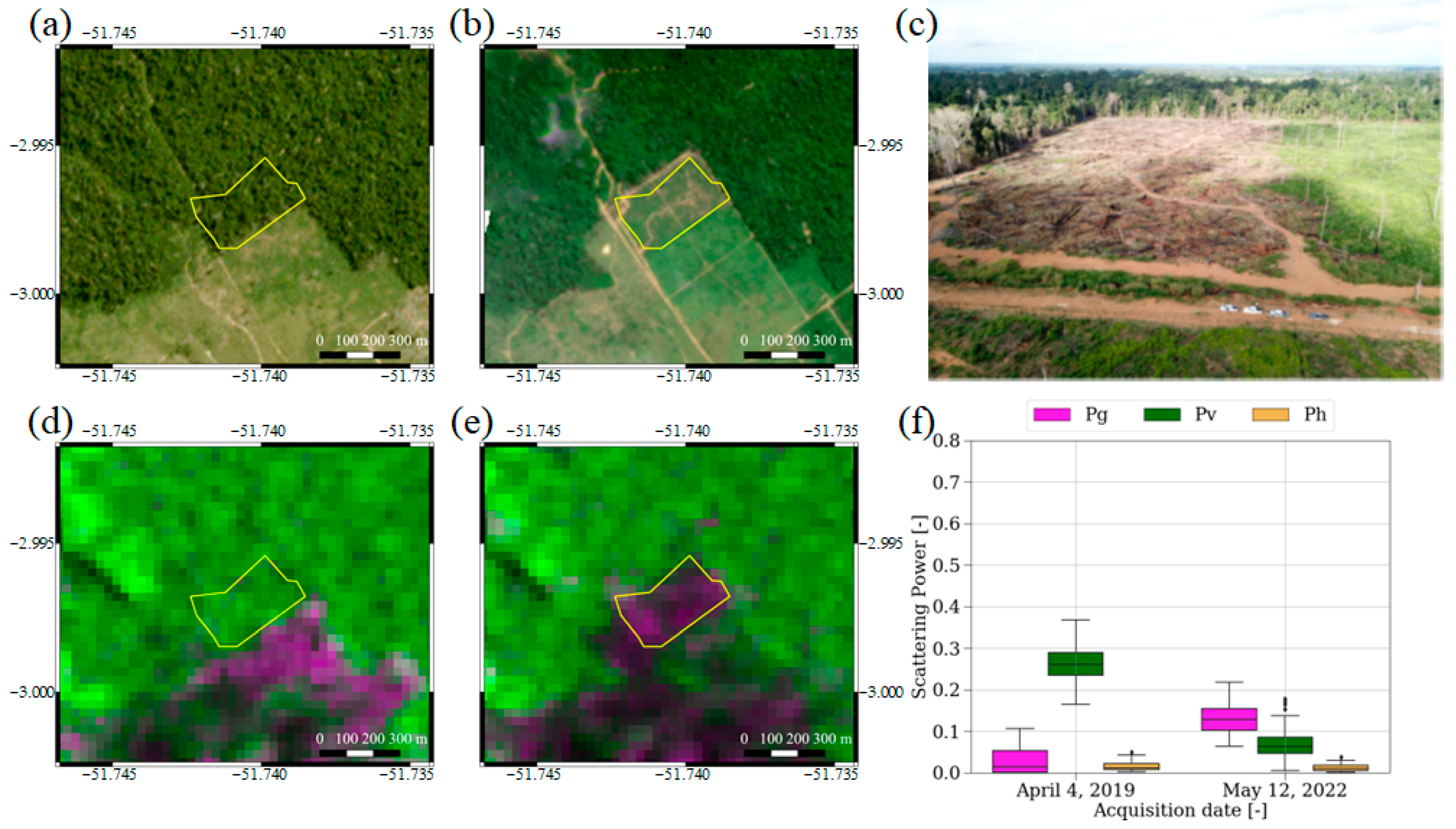
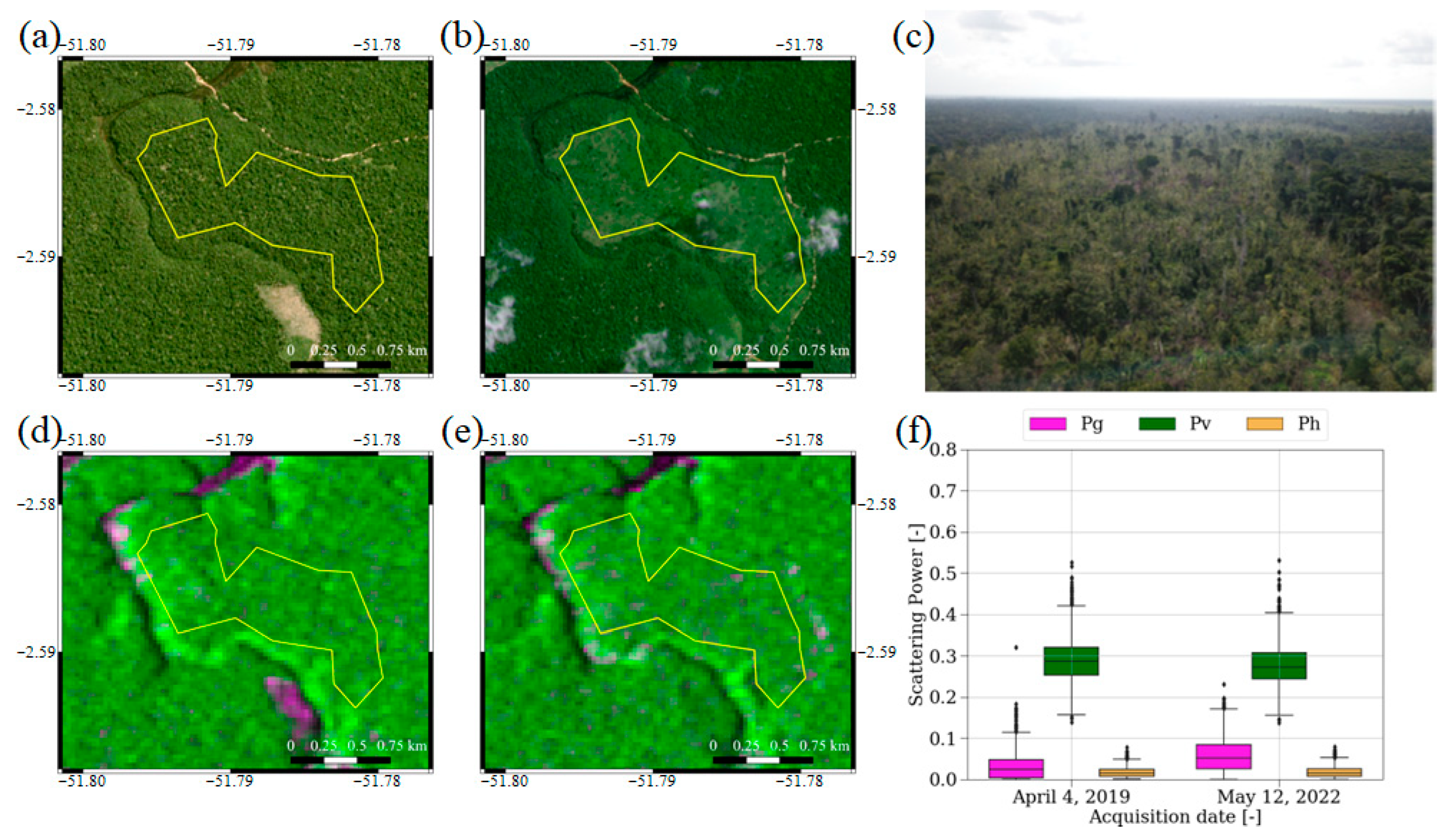
3.4. Application to Actual Dual-Polarization Data
4. Discussion
5. Conclusions
Author Contributions
Funding
Data Availability Statement
Acknowledgments
Conflicts of Interest
References
- IPCC. Climate Change 2022: Mitigation of Climate Change. Contribution of Working Group III to the Fifth Assessment Report of the Intergovernmental Panel on Climate Change; IPCC: Geneva, Switzerland, 2022. [Google Scholar]
- FAO. Global Forest Resources Assessment 2020-Main Report; Food and Agricultural Organization, FAO: Rome, Italy, 2020. [Google Scholar]
- Silva Junior, C.H.L.; Pessôa, A.C.M.; Carvalho, N.S.; Reis, J.B.C.; Anderson, L.O.; Aragão, L.E.O.C. The Brazilian Amazon deforestation rate in 2020 is the greatest of the decade. Nat. Ecol. Evol. 2021, 5, 144–145. [Google Scholar] [CrossRef]
- Potapov, P.V.; Turubanova, S.A.; Hansen, M.C.; Adusei, B.; Broich, M.; Altstatt, A.; Mane, L.; Justice, C.O. Quantifying forest cover loss in Democratic Republic of the Congo, 2000–2010, with Landsat ETM+ data. Remote Sens. Environ. 2012, 122, 106–116. [Google Scholar]
- Nikonovas, T.; Spessa, A.; Doerr, S.H.; Clay, G.D.; Mezbahuddin, S. Near-complete loss of fire-resistant primary tropical forest cover in Sumatra and Kalimantan. Commun. Earth Environ. 2020, 1, 65. [Google Scholar] [CrossRef]
- Watanabe, M.; Koyama, C.N.; Hayashi, M.; Nagatani, I.; Tadono, T.; Shimada, M. Refined algorithm for forest early warning system with ALOS-2/PALSAR-2 ScanSAR data in tropical forest regions. Remote Sens. Environ. 2021, 265, 112643. [Google Scholar] [CrossRef]
- Reiche, J.; Mullissa, A.; Slagter, B.; Gou, Y.; Tsendbazar, N.E.; Odongo-Braun, C.; Vollrath, A.; Weisse, M.J.; Stolle, F.; Pickens, A.; et al. Forest disturbance alerts for the Congo Basin using Sentinel-1. Environ. Res. Lett. 2021, 16, 24005. [Google Scholar]
- Sugimoto, R.; Kato, S.; Nakamura, R.; Tsutsumi, C.; Yamaguchi, Y. Deforestation detection using scattering power decomposition and optimal averaging of volume scattering power in tropical rainforest regions. Remote Sens. Environ. 2022, 275, 113018. [Google Scholar] [CrossRef]
- Takeshi, M.; Yukihiro, K.; Satoko, M.; Shinichi, S. ALOS-4 L-Band SAR Observation Concept and Development Status. In Proceedings of the 2020 IEEE International Geoscience and Remote Sensing Symposium, Waikoloa, HI, USA, 26 September–2 October 2020. [Google Scholar]
- Cloude, S.R. The Dual Polarization Entropy/Alpha Decomposition: A PALSAR Case Study. In Proceedings of the 3rd International Workshop on Science and Applications of SAR Polarimetry and Polarimetric Interferometry, Frascati, Italy, 1 March 2007. [Google Scholar]
- Ji, K.; Wu, Y. Scattering Mechanism Extraction by a Modified Cloude-Pottier Decomposition for Dual Polarization SAR. Remote Sens. 2015, 7, 7447–7470. [Google Scholar] [CrossRef]
- Rosenqvist, A.; Shimada, M.; Suzuki, S.; Ohgushi, F.; Tadono, T.; Watanabe, M.; Tsuzuku, K.; Watanabe, T.; Kamijo, S.; Aoki, E. Operational performance of the ALOS global systematic acquisition strategy and observation plans for ALOS-2 PALSAR-2. Remote Sens. Environ. 2014, 155, 3–12. [Google Scholar] [CrossRef]
- Moriyama, T. Polarimetric calibration of PALSAR2. In Proceedings of the 2015 IEEE International Geoscience and Remote Sensing Symposium, Milan, Italy, 26–31 July 2015. [Google Scholar]
- Koyama, C.N.; Watanabe, M.; Hayashi, M.; Ogawa, T.; Shimada, M. Mapping the spatial-temporal variability of tropical forests by ALOS-2 L-band SAR big data analysis. Remote Sens. Environ. 2019, 233, 111372. [Google Scholar] [CrossRef]
- Freeman, A.; Durden, S.L. A three-component scattering model for polarimetric SAR data. IEEE Trans. Geosci. Remote Sens. 1998, 36, 963–973. [Google Scholar] [CrossRef]
- Singh, G.; Yamaguchi, Y.; Park, S.-E. General four-component scattering power decomposition with unitary transformation of coherency matrix. IEEE Trans. Geosci. Remote Sens. 2013, 51, 3014–3022. [Google Scholar]
- Singh, G.; Yamaguchi, Y. Model-based six-component scattering matrix power decomposition. IEEE Trans. Geosci. Remote Sens. 2018, 56, 5687–5704. [Google Scholar] [CrossRef]
- Yamaguchi, Y. Polarimetric SAR Imaging: Theory and Applications; CRC Press: Boca Raton, FL, USA, 2020. [Google Scholar]
- Almeida-Filho, R.; Shimabukuro, Y.E.; Rosenqvist, A.; Sánchez, G.A. Using dual-polarized ALOS PALSAR data for detecting new fronts of deforestation in the Brazilian Amazônia. Int. J. Remote Sens. 2009, 30, 3735–3743. [Google Scholar] [CrossRef]
- Kim, Y.; van Zyl, J.J. A time-series approach to estimate soil moisture using polarimetric radar data. IEEE Trans. Geosci. Remote Sens. 2009, 47, 2519–2527. [Google Scholar]
- Charbonneau, F.; Trudel, M.; Fernandes, R. Use of Dual Polarization and Multi-Incidence SAR for soil permeability mapping. In Proceedings of the 2005 Advanced Synthetic Aperture Radar (ASAR) Workshop, St-Hubert, QC, Canada, 15–17 November 2005. [Google Scholar]
- Shimada, M.; Itoh, T.; Motooka, T.; Watanabe, M.; Shiraishi, T.; Thapa, R.; Lucas, R. New Global Forest/Non-forest Maps from ALOS PALSAR Data (2007-2010). Remote Sens. Environ. 2014, 155, 13–31. [Google Scholar] [CrossRef]
- Shimada, M.; Ohtaki, T. Generating Large-Scale High-Quality SAR Mosaic Datasets: Application to PALSAR Data for Global Monitoring. IEEE J. Sel. Top Appl. Earth Obs. Remote Sens. 2010, 3, 637–656. [Google Scholar] [CrossRef]


| Site | Subarea | Off-Nadir Angle (°) | Acquisition Date |
|---|---|---|---|
| Rio Branco | A | 28.4° | 9 January 2015 |
| 19 January 2018 | |||
| B | 30.9° | 23 January 2015 | |
| 5 January 2018 | |||
| Ucayali River | – | 30.9° | 16 April 2016 |
| Kalimantan | A | 33.2° | 9 January 2016 |
| 29 October 2016 | |||
| B | 28.4° | 8 December 2014 | |
| 27 April 2015 | |||
| Congo Basin | A | 28.4° | 8 November 2014 |
| 7 May 2016 | |||
| B | 8 November 2014 | ||
| 7 May 2016 |
| Polygons | Pixels | Area (ha) | |
|---|---|---|---|
| Deforestation | 406 | 21,281 | 1915 |
| Permanent forest | 514 | 341,355 | 30,722 |
| Permanent non-forest | 648 | 394,589 | 35,513 |
| Symbol | Description | Equation | Theoretical Value for Forest |
|---|---|---|---|
| RFDI | Radar forest degradation index | 0.5 | |
| RVI | Radar vegetation index | 1.0 |
| Method and Data | Window Size for Ensemble Average | UA (%) | PA (%) | Kappa | |
|---|---|---|---|---|---|
| Proposed method with HH/HV | 7 × 14 pixels | 0.15 | 98.6 | 99.3 | 0.981 |
| 10 × 20 pixels | 0.16 | 98.6 | 99.5 | 0.983 | |
| 14 × 28 pixels | 0.17 | 98.8 | 99.5 | 0.984 | |
| Proposed method with VV/VH | 7 × 14 pixels | 0.15 | 98.6 | 99.3 | 0.980 |
| 10 × 20 pixels | 0.16 | 98.6 | 99.4 | 0.982 | |
| 14 × 28 pixels | 0.17 | 98.8 | 99.4 | 0.983 | |
| 6SD method with POLSAR | 7 × 14 pixels | 0.20 | 98.5 | 99.2 | 0.979 |
| 10 × 20 pixels | 0.24 | 98.6 | 99.6 | 0.982 | |
| 14 × 28 pixels | 0.28 | 98.8 | 99.5 | 0.984 |
| Method and Data | Window Size for Ensemble Average | Threshold | UA (%) | PA (%) | Kappa | |
|---|---|---|---|---|---|---|
| Proposed method with HH/HV | 7 × 14 pixels | 0.16 | –0.04 | 88.7 | 68.9 | 0.770 |
| 10 × 20 pixels | 0.17 | –0.04 | 92.1 | 69.9 | 0.789 | |
| 14 × 28 pixels | 0.18 | –0.04 | 93.3 | 71.0 | 0.802 | |
| Proposed method with VV/VH | 7 × 14 pixels | 0.16 | –0.04 | 90.2 | 67.3 | 0.765 |
| 10 × 20 pixels | 0.17 | –0.04 | 93.2 | 68.9 | 0.787 | |
| 14 × 28 pixels | 0.18 | –0.04 | 94.8 | 69.7 | 0.799 | |
| 6SD method with POLSAR | 7 × 14 pixels | 0.21 | –0.06 | 83.2 | 67.9 | 0.741 |
| 10 × 20 pixels | 0.26 | –0.07 | 90.5 | 70.2 | 0.786 | |
| 14 × 28 pixels | 0.30 | –0.07 | 92.3 | 71.8 | 0.803 | |
| Site | Subarea | Acquisition Date | UA (%) | PA (%) | Kappa | |
|---|---|---|---|---|---|---|
| Proposed method with HH/HV | ||||||
| Ucayali River | – | 16 April 2016 | 0.14 | 98.3 | 97.1 | 0.867 |
| Kalimantan | A | 9 January 2016 | 0.14 | 92.1 | 89.9 | 0.875 |
| 29 October 2016 | 0.13 | 87.4 | 95.4 | 0.859 | ||
| B | 8 December 2014 | 0.13 | 95.7 | 98.9 | 0.844 | |
| 27 April 2015 | 0.13 | 95.6 | 98.8 | 0.848 | ||
| Congo Basin | A | 8 November 2014 | 0.13 | 94.9 | 98.9 | 0.861 |
| 7 May 2016 | 0.13 | 94.6 | 98.4 | 0.865 | ||
| B | 8 November 2014 | 0.14 | 85.2 | 91.1 | 0.838 | |
| 7 May 2016 | 0.13 | 81.1 | 96.4 | 0.843 | ||
| Proposed method with VV/VH | ||||||
| Ucayali River | – | 16 April 2016 | 0.16 | 92.2 | 99.5 | 0.682 |
| Kalimantan | A | 9 January 2016 | 0.13 | 86.8 | 95.1 | 0.869 |
| 29 October 2016 | 0.13 | 85.4 | 95.6 | 0.842 | ||
| B | 8 December 2014 | 0.13 | 94.6 | 98.8 | 0.806 | |
| 27 April 2015 | 0.13 | 94.1 | 98.9 | 0.801 | ||
| Congo Basin | A | 8 November 2014 | 0.13 | 94.0 | 99.1 | 0.839 |
| 7 May 2016 | 0.13 | 93.8 | 98.3 | 0.845 | ||
| B | 8 November 2014 | 0.14 | 81.1 | 90.3 | 0.801 | |
| 7 May 2016 | 0.13 | 78.1 | 95.3 | 0.814 | ||
| Method and Data | Window Size for Ensemble Average | Threshold | UA (%) | PA (%) | Kappa | |
|---|---|---|---|---|---|---|
| RFDI with HH/HV | 7 × 14 pixels | 0.34 | 0.61 | 95.6 | 97.2 | 0.933 |
| 10 × 20 pixels | 0.34 | 0.61 | 96.0 | 97.7 | 0.940 | |
| 14 × 28 pixels | 0.38 | 0.60 | 97.1 | 97.0 | 0.946 | |
| RFDI with VV/VH | 7 × 14 pixels | 0.38 | 0.58 | 86.0 | 96.8 | 0.824 |
| 10 × 20 pixels | 0.40 | 0.57 | 88.2 | 95.6 | 0.840 | |
| 14 × 28 pixels | 0.42 | 0.57 | 88.8 | 96.9 | 0.857 | |
| RVI with HH/HV | 7 × 14 pixels | 0.79 | – | 96.2 | 96.7 | 0.933 |
| 10 × 20 pixels | 0.79 | – | 96.4 | 97.2 | 0.940 | |
| 14 × 28 pixels | 0.79 | – | 96.7 | 97.5 | 0.946 | |
| RVI with VV/VH | 7 × 14 pixels | 0.85 | – | 86.9 | 95.6 | 0.825 |
| 10 × 20 pixels | 0.85 | – | 87.3 | 96.9 | 0.840 | |
| 14 × 28 pixels | 0.86 | – | 88.7 | 96.9 | 0.857 | |
| Method and Data | UA (%) | PA (%) | Kappa | |
|---|---|---|---|---|
| Proposed method with HH/HV | 0.10 | 97.5 | 98.0 | 0.959 |
| Proposed method with VV/VH | 0.11 | 98.0 | 98.2 | 0.964 |
| 6SD method with POLSAR | 0.11 | 97.4 | 59.0 | 0.592 |
Disclaimer/Publisher’s Note: The statements, opinions and data contained in all publications are solely those of the individual author(s) and contributor(s) and not of MDPI and/or the editor(s). MDPI and/or the editor(s) disclaim responsibility for any injury to people or property resulting from any ideas, methods, instructions or products referred to in the content. |
© 2023 by the authors. Licensee MDPI, Basel, Switzerland. This article is an open access article distributed under the terms and conditions of the Creative Commons Attribution (CC BY) license (https://creativecommons.org/licenses/by/4.0/).
Share and Cite
Sugimoto, R.; Nakamura, R.; Tsutsumi, C.; Yamaguchi, Y. Extension of Scattering Power Decomposition to Dual-Polarization Data for Tropical Forest Monitoring. Remote Sens. 2023, 15, 839. https://doi.org/10.3390/rs15030839
Sugimoto R, Nakamura R, Tsutsumi C, Yamaguchi Y. Extension of Scattering Power Decomposition to Dual-Polarization Data for Tropical Forest Monitoring. Remote Sensing. 2023; 15(3):839. https://doi.org/10.3390/rs15030839
Chicago/Turabian StyleSugimoto, Ryu, Ryosuke Nakamura, Chiaki Tsutsumi, and Yoshio Yamaguchi. 2023. "Extension of Scattering Power Decomposition to Dual-Polarization Data for Tropical Forest Monitoring" Remote Sensing 15, no. 3: 839. https://doi.org/10.3390/rs15030839
APA StyleSugimoto, R., Nakamura, R., Tsutsumi, C., & Yamaguchi, Y. (2023). Extension of Scattering Power Decomposition to Dual-Polarization Data for Tropical Forest Monitoring. Remote Sensing, 15(3), 839. https://doi.org/10.3390/rs15030839