Gradual Domain Adaptation with Pseudo-Label Denoising for SAR Target Recognition When Using Only Synthetic Data for Training

Abstract

Because of the high cost of data acquisition in synthetic aperture radar (SAR) target recognition, the application of synthetic (simulated) SAR data is becoming increasingly popular. Our study explores the problems encountered when training fully on synthetic data and testing on measured (real) data, and the distribution gap between synthetic and measured SAR data affects recognition performance under the circumstances. We propose a gradual domain adaptation recognition framework with pseudo-label denoising to solve this problem. As a warm-up, the feature alignment classification network is trained to learn the domain-invariant feature representation and obtain a relatively satisfactory recognition result. Then, we utilize the self-training method for further improvement. Some pseudo-labeled data are selected to fine-tune the network, narrowing the distribution difference between the training data and test data for each category. However, the pseudo-labels are inevitably noisy, and the wrong ones may deteriorate the classifier’s performance during fine-tuning iterations. Thus, we conduct pseudo-label denoising to eliminate some noisy pseudo-labels and improve the trained classifier’s robustness. We perform pseudo-label denoising based on the image similarity to keep the label consistent between the image and feature domains. We conduct extensive experiments on the newly published SAMPLE dataset, and we design two training scenarios to verify the proposed framework. For Training Scenario I, the framework matches the result of neural architecture searching and achieves 96.46% average accuracy. For Training Scenario II, the framework outperforms the results of other existing methods and achieves 97.36% average accuracy. These results illustrate the superiority of our framework, which can reach state-of-the-art recognition levels with appropriate stability.

1. Introduction

Synthetic aperture radar (SAR) data have been widely used in many fields, such as military surveillance, disaster warning, and environmental monitoring. SAR automatic target recognition (SAR-ATR) technology, which aims to recognize the target types of SAR images, has been comprehensively studied in the literature. With the popularity of deep learning methods in recent years, they have been effectively used for SAR-ATR, and a large amount of training data are usually needed to ensure the reliability of the trained deep models. However, due to the particularity of SAR images, the cost of acquiring a large amount of labeled SAR data is high, and a lack of training data will influence the recognition performance of the deep models [1,2,3,4,5].

Many research works have been conducted on SAR target recognition regarding cases of insufficient training data or few-shot learning [3,4,5,6,7,8,9,10,11,12,13,14,15,16,17,18,19,20,21]. In general, these methods can be divided into the following categories: (1) Data augmentation can be used to increase the number of training samples. There are traditional data augmentation methods, such as the translation of the target and adding random speckle noise used in [6,7], and deep generative methods, such as generating images by Wasserstein generative adversarial networks with a gradient penalty [12] or by adversarial autoencoder [13]. (2) More robust features can be designed, which helps to improve recognition accuracy. There are traditional features, such as the sparse representation of the monogenic signal [8] and modified polar mapping [9], as well as features extracted by deep networks, such as deep highway unit [10], attribute-guided multi-scale prototypical network [11], angular rotation generative networks [5], and convolutional transformers [16]. (3) Transfer learning methods can be applied [3,4,5]. In this situation, auxiliary datasets can be used for transferring relevant knowledge [5] or pre-training the network [3,4]. (4) Other methods, such as semi-supervised learning methods [3,15,17,18,19,20,21] or meta-learning methods [11,14], can also be applied to the few-shot learning problem. The above methods can be combined for better results when the training data is scant.

Because the data acquisition of measured (real) SAR data is usually difficult, a growing number of studies [1,2,22,23,24,25,26,27,28,29,30,31,32,33,34,35,36] have been conducted that utilize synthetic (simulated) SAR data for the recognition problem. The Moving and Stationary Target Acquisition and Recognition (MSTAR) dataset [37] provided by the Air Force Research Laboratory (AFRL), USA, has been widely used in the development of SAR-ATR algorithms over the past two decades. A dataset called the Synthetic and Measured Paired Labeled Experiment (SAMPLE) has also been introduced by AFRL to solve synthetic SAR target recognition problems [24]. In our paper, we conduct experiments on the SAMPLE dataset.

The research works based on the synthetic SAR data for recognition problems can be roughly divided into these main categories: (1) Pre-training: using plentiful synthetic SAR data to pre-train the classifier, and then using a small amount of measured SAR data to fine-tune the pre-trained network [1]; (2) Transformation or augmenting: transforming or augmenting the synthetic data to train the classifier to achieve better recognition results [2,22,23,24,25,26,29,34,35]; (3) Designing features: designing more general features [28,30,32,33,36] for training, such as ensembling traditional features [28], features based on scattering centers [32], or multi-scale deep features [36]. (4) Domain adaptation methods: adding some domain adaptation constraints for optimization, which makes the trained classifier more suitable for measured data [27,36]; (5) Other methods: such as neural architecture searching [31], or exploring the effectiveness of the existing methods and integrating some effective methods [25].

Considering the research works that use synthetic SAR data for recognition, there are two main recognition situations. First recognition situation: large and small amounts of synthetic and measured data, respectively, are labeled for training [1,2,22,29,35]. Second recognition situation: there are only synthetic data with labels for training, and the measured data of the same categories as the synthetic data are used as the test data [23,24,25,26,27,28,30,31,32,33,34,36]. The second recognition situation is more challenging. In our paper, we also consider the second recognition situation which is training fully on the synthetic SAR data and testing on the measured data, and the main challenge when training fully on the synthetic SAR data and testing on the measured data is the distribution gap between the training and test data.

In this paper, we design a gradual domain adaptation recognition framework with pseudo-label denoising to solve the distribution gap problem and achieve state-of-the-art recognition performance using the SAMPLE dataset. The existing methods [27,36] based on the domain adaptation idea only consider the feature alignment between different domains, while we utilize the self-training method further to narrow the distribution difference of the training data and test data for each category. 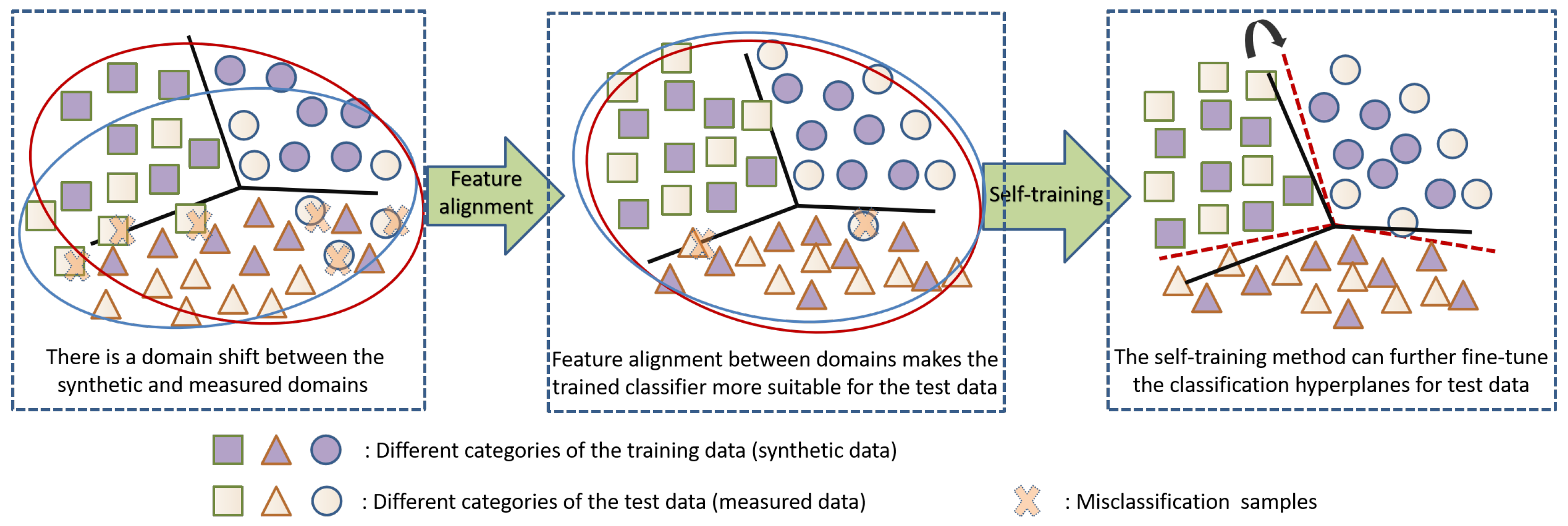Figure 1 illustrates the gradual domain adaptation process which contains two stages, i.e., feature alignment classification and self-training. The two stages are explained as follows. For the first stage, there is a domain shift between the original features of the training data and the test data, and feature alignment narrows the feature distance to learn the domain-invariant features. For the second stage of self-training, the classification boundaries are further modified to fit the pseudo-labeled test data, which can also align the distribution of each category between the synthetic training data and the measured test data, thus enhancing the classification performance. The contributions of this paper can be summarized as follows:

(1)

We design the two-stage gradual domain adaptation framework. Warm-up stage: training the feature alignment classification network to obtain the domain-invariant feature representation and a high-precision initialized classification result. Fine-tuning stage: selecting some pseudo-labeled data to fine-tune the classifier, and it actually narrows the distribution difference between the training data and test data for each category.

(2)

We propose a pseudo-label denoising method to eliminate some falsely pseudo-labeled data, while falsely pseudo-labeled data negatively influence the fine-tuning stage. We use image similarity to measure the similarity of the pseudo-labeled data, and then keep the label consistent between the images of high similarities. The technique is simple and effective for improving the accuracy of the pseudo-labeled data, thus improving the final classification performance of the whole framework.

(3)

We evaluate the whole framework on the newly published SAMPLE data set. The experimental results on the SAMPLE dataset illustrate that our proposed framework is practical and our proposed method can obtain state-of-the-art recognition accuracy.

The rest of our paper is arranged as follows: in Section 2, we briefly review some related works; in Section 3, we introduce the gradual domain adaptation recognition framework and the pseudo-label denoising method; we provide the experimental setups and results in Section 4; finally, in Section 5 and Section 6, we give some discussions and draw some conclusions, respectively.

2. Related Work

2.1. Transfer Learning and Unsupervised Domain Adaptation

Transfer learning [38,39] relaxes the hypothesis that the training data must be independent and identically distributed (i.i.d.) with the test data, and therefore, it can be used to solve the problem of insufficient training data. There are two domains for transfer learning problems: source domain $D_s$ and target domain $D_t$.

Domain adaptation [40,41] is a type of transductive transfer learning, which means that the source task $T_s$ in the source domain and the target task $T_t$ in the target domain are the same, i.e., $T_s=T_t$, while the differences are only caused by domain divergence, $D_s\ne D_t$. Domain adaptation aims to utilize the labeled source data to improve the performance of the target task $T_t$.

Unsupervised domain adaptation is defined as a case in which labeled source data and unlabeled target data are available [41]. These unsupervised domain adaptation methods include aligning the feature distributions of different domains [42,43,44], designing different normalized statistics of different domains [45,46], and utilizing ensemble-based methods [47,48] or adversarial training [49,50]. The aforementioned methods can also be combined for the unsupervised domain adaptation problem.

2.2. Semi-Supervised Learning

Only labeled data are used to train the classifier for supervised learning. The classifier’s performance depends on the sample size of training data to some extent. However, obtaining abundant labeled data is usually difficult, expensive, or time-consuming. Meanwhile, unlabeled data are relatively easier to obtain. Thus, semi-supervised learning [51,52] is popular because it can make use of unlabeled data.

Some studies [3,15,17,18,19,20,21] have utilized semi-supervised methods for SAR-ATR, mainly in the absence of labeled data. Zhang et al. proposed a semi-supervised method based on generative adversarial networks, which makes it capable of learning the feature representation of unlabeled input data [3]. Gao et al. used the active learning method to label some informative samples. They develop a semi-supervised strategy by adding a new regularization term to the loss functions of convolutional neural networks (CNN) [15]. An end-to-end semi-supervised recognition method based on an attention mechanism and bias-variance decomposition has also been proposed, focusing on unlabeled data screening and assigning pseudo-labels [17]. Wang et al. combined the contrastive learning method with pseudo-labels for the few-shot SAR-ATR [18]. A semi-supervised learning framework, which includes a self-consistent augmentation rule, a mix-up-based mixture, and weighted loss, has also been proposed [20]. Additionally, Liu et al. proposed a semi-supervised conditional generative adversarial network with multi-discriminators, which can discriminate the generated images and predict the labels for unlabeled samples [21].

2.3. Pseudo-Label Denoising

Self-training [53] is also known as the pseudo-label method. The basic idea of self-training is taking the pseudo-labeled samples for training until the prediction results of the classifier no longer change. Self-training performance depends on the correctness of the pseudo-labels provided by the initially trained classifier. When the noisy pseudo-labels are used for fine-tuning, the classifier may make more mistakes during the fine-tuning process. Furthermore, some noisy pseudo-labels will inevitably exist even with an initial high-precision classifier. Thus, pseudo-label denoising is essential for improving the performance of the self-training process.

In recent years, researchers [54,55,56,57] have considered how to de-noise false labels for SAR image classification. Wang et al. proposed a loss curve-fitting-based method to identify the noisy labels and effectively train the classification network [54]. Multi-classifiers are combined to keep the label consistent and eliminate noise [55]. Probability transition CNN has also been proposed for patch-level SAR image land-cover classification with noisy labels [56]. Shang et al. [57] proposed a SAR image segmentation method using region smoothing and label correction to correct the misclassified pixels in the image.

3. Gradual Domain Adaptation Recognition Framework

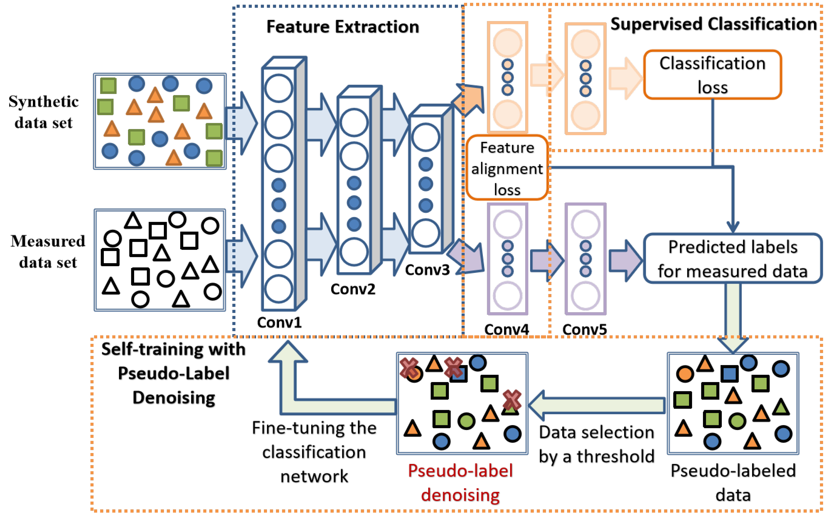
We propose a gradual domain adaptation recognition framework with pseudo-label denoising to solve the distribution gap problem and make the classifier trained by the training data more applicable to the test data. The flowchart of the whole algorithm is illustrated in Figure 2 below. Synthetic dataset $X_L$ is in the source domain and measured dataset $X_U$ is in the target domain. The recognition task is training on the $X_L$ and then testing on the $X_U$. Since there is a distribution difference between the synthetic data and the measured data, we use a feature alignment classification network $\mathcal{F}$ to learn the domain-invariant feature representation for classification. Then, some pseudo-labeled data $X_{deno}$ from $X_U$ are selected by pre-set threshold and pseudo-labeled denoising method. $X_L\cup X_{deno}$ are used to fine-tune the $\mathcal{F}$ for a better result.

In this section, we first introduce a basic recognition network; then, we introduce the gradual domain adaptation recognition framework, which contains two domain adaptation stages: the feature alignment classification network and the self-training method; finally, we also present the proposed pseudo-label denoising method, which we carry out in the self-training process. The detailed introductions are given below.

3.1. Basic Recognition Network

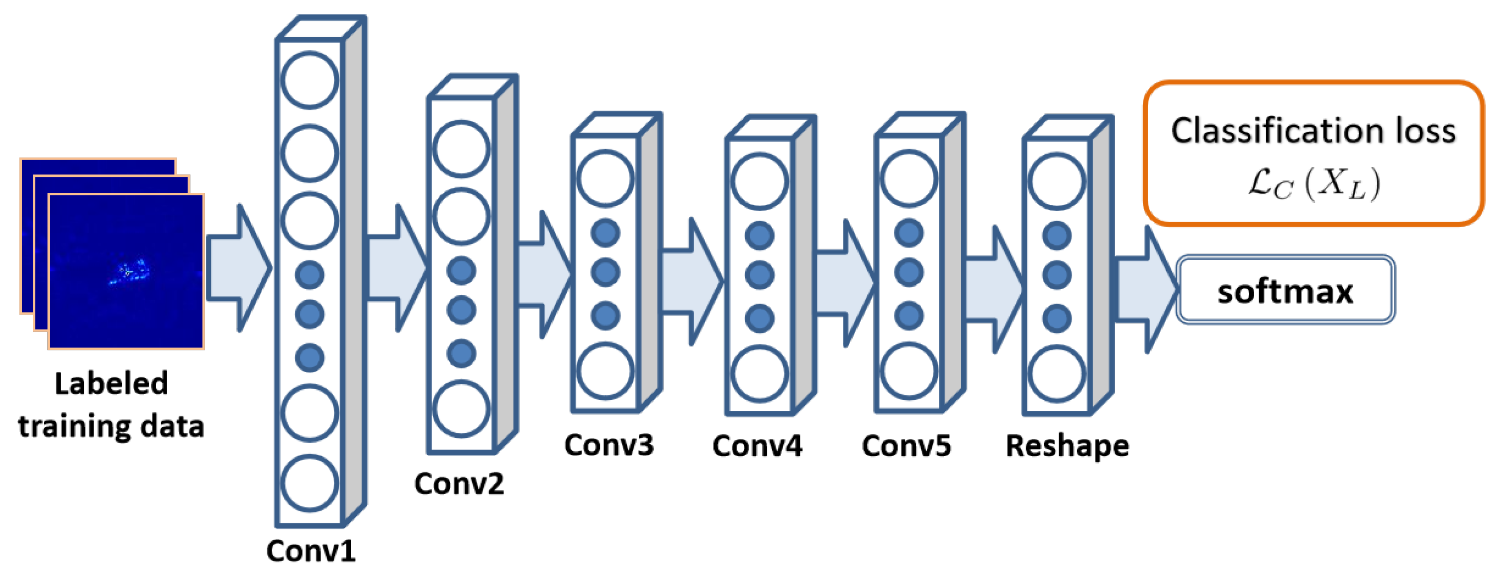
A previous study [31] demonstrated that too deep network structures might not generalize well when there is a domain shift between the training and test data. Thus, we think that the five-layer network structure is sufficient to extract the deep distinguishing features because A-ConvNets have achieved state-of-the-art recognition accuracy for the ten-class MSTAR recognition problem [6]. As shown in Figure 3, we refer to A-ConvNets when designing the basic recognition network and modify the kernel sizes to fit the image sizes.

Here, we introduce the architecture of the basic recognition network. The network has a five-layer all-convolutional architecture, and there is a dropout [58,59] operation after the fourth convolutional layer. The kernel size of the first four layers is 5 × 5, and the kernel size of the fifth layer is 4 × 4. We parameterize the 5-layer basic recognition network as $\varphi (·;\mathbf{\vartheta })$, and $\mathbf{\vartheta }$ represents the corresponding parameters.

For an input sample $\mathbf{x}$ with the real category label $\mathbf{y}$ of the one-hot form, the predicted label of the recognition network can be expressed as a 10-dimensional vector $\widehat{\mathbf{y}}=\varphi (\mathbf{x};\mathbf{\vartheta })$. The specific expression is given as follows:

$$\widehat{\mathbf{y}}=[{\widehat{y}}_1,{\widehat{y}}_2,\dots ,{\widehat{y}}_K]$$

(1)

where ${\widehat{y}}_i$ is the ith-dimensional value of vector $\widehat{\mathbf{y}}$, which indicates the probability of the sample $\mathbf{x}$ belonging to the i-th category. K is the number of categories, and $K=10$ in our experiment.

The classification loss ${\mathcal{L}}_C\left(X_L\right)$, which is actually cross entropy loss [60], is calculated on the labeled synthetic dataset $X_L$:

$${\mathcal{L}}_C\left(X_L\right)=E_{X_L}[\sum _{i=1}^K-y_{i}log{\widehat{y}}_i]$$

(2)

where $y_i$ is the ith-dimensional value of the real category vector $\mathbf{y}$.

3.2. Stage One: Feature Alignment Classification Network

As we can see in Figure 3, a recognition network $\varphi (·;\mathbf{\vartheta })$ is usually trained on the labeled training dataset $X_L$. Thus, when there is a distribution gap between the training and test data, the trained network may not fit well with the test dataset $X_U$.

We design a feature alignment classification network $\mathcal{F}$ to learn a domain-invariant feature representation for a better recognition result. Figure 4 gives the illustration of the feature alignment classification network, and an earlier version is introduced in Ref. [36]. However, while the earlier version utilizes a multi-scale deep network as the feature extractor, we use the all-convolutional architecture as the feature extractor.

Figure 4 shows that the network parameters are shared for the labeled synthetic dataset $X_L$ and unlabeled measured dataset $X_U$. The classification loss ${\mathcal{L}}_C\left(X_L\right)$ is calculated on the labeled synthetic dataset, and the feature alignment restriction $\mathcal{D}(X_L,X_U)$ is calculated between the fourth-layer features of $X_L$ and $X_U$. ${\mathbf{x}}_l$ and ${\mathbf{x}}_u$ represent the corresponding samples in the labeled synthetic data set $X_L$ and unlabeled measured data set $X_U$, respectively.

The deep features of the fourth layer are expressed as $f\left({\mathbf{x}}_l\right)$ and $f\left({\mathbf{x}}_u\right)$. The feature alignment loss between the features of the synthetic and measured datasets can be simply expressed as follows [36,42]:

$$\mathcal{D}\left(X_L,X_U\right)=\parallel E_{X_L}\left[f\left({\mathbf{x}}_l\right)\right]-E_{X_U}\left[f\left({\mathbf{x}}_u\right)\right]\parallel$$

(3)

Thus, the total loss function of the feature alignment classification network can be expressed as follows:

$$\mathcal{L}={\mathcal{L}}_C\left(X_L\right)+\lambda \mathcal{D}\left(X_L,X_U\right)$$

(4)

where $\lambda$ determines the proportion of feature alignment loss in the total loss $\mathcal{L}$.

As a warm-up, the feature alignment classification network $\mathcal{F}$ is trained to optimize the total loss function to learn the domain-invariant feature representation. The optimization of classification loss ensures an effective recognition performance on the synthetic training dataset $X_L$, while the optimization of the feature alignment loss can narrow the feature difference between the training and test data, thereby improving the classification result on the measured test dataset $X_U$.

3.3. Stage Two: Self-Training

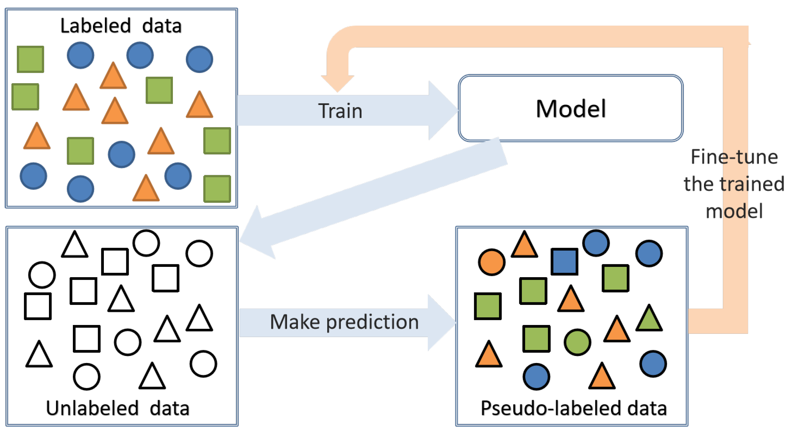
Self-training is a common semi-supervised learning method, and it can also be utilized for further domain adaptation to narrow the distribution difference between the training and test data for each category. Figure 5 shows the self-training process.

A classifier is initially trained on the labeled dataset $X_L$ to obtain the prediction on the unlabeled dataset $X_U$. Then, some pseudo-labeled measured data $X_{pre}$ are selected, and in the self-training process, the measured data with the pseudo-labels and labeled synthetic data $X_{pre}\cup X_L$ are used to train the classifier together. Since the classifier has seen the measured data with the pseudo-labels and labeled synthetic data, the boundaries of the trained classifier are modified to fit the measured data better, which can also align the feature of the same categories in synthetic and measured domains.

When the feature alignment classification network $\mathcal{F}$ has been well trained and given an unlabeled measured sample ${\mathbf{x}}_u$, the predicted pseudo-label ${\widehat{\mathbf{y}}}_u$ can be obtained:

$${\widehat{\mathbf{y}}}_u=\varphi ({\mathbf{x}}_u;\mathbf{\vartheta })=[{\widehat{y}}_{u1},{\widehat{y}}_{u2},\dots ,{\widehat{y}}_{uK}]$$

(5)

$$p_{pred}=max\{{\widehat{y}}_{u1},{\widehat{y}}_{u2},\dots ,{\widehat{y}}_{uK}\}$$

(6)

$p_{pred}$ indicates the probability of the sample ${\mathbf{x}}_u$ belonging to the predicted category.

The threshold value $\gamma$ is set and some pseudo-labeled data are selected as the $X_{pre}$ to fine-tune the whole network. For a pseudo-labeled sample (${\mathbf{x}}_u$, ${\widehat{\mathbf{y}}}_u$), if $p_{pred}>\gamma$, it is selected; otherwise, it is not selected. We use the predicted soft labels as the pseudo-labels for fine-tuning, which means that the classification loss ${\mathcal{L}}_C$ calculated on the pseudo-labeled dataset $X_{pre}$ can be expressed as follows:

$${\mathcal{L}}_C\left(X_{pre}\right)=E_{X_{pre}}[\sum _{i=1}^K-{\widehat{y}}_{ui}log{\tilde{y}}_{ui}]$$

(7)

where ${\tilde{\mathbf{y}}}_u=[{\tilde{y}}_{u1},{\tilde{y}}_{u2},\dots ,{\tilde{y}}_{uK}]$ is the newly predicted label for sample ${\mathbf{x}}_u$ after fine-tuning. The pseudo-labels are constantly updated.

In the fine-tuning process, the total loss function can be expressed as follows:

$$\mathcal{L}={\mathcal{L}}_C\left(X_L\right)+\lambda \mathcal{D}\left(X_L,X_U\right)+{\mathcal{L}}_C\left(X_{pre}\right)$$

(8)

we can see that in the self-training process, the classification loss is calculated on the $X_L$ and $X_{pre}$.

The performance of the self-training method mainly depends on the initially trained classifier. We design the feature alignment classification network $\mathcal{F}$ as the initially trained classifier for a better recognition result. However, the pseudo-labeled dataset selected by the threshold $\gamma$ is not entirely accurate and reliable. The correctness of pseudo-labels is also related to the recognition performance of the test data. Since the recognition result of the test data is not perfectly correct, the pseudo-labels of the test data are also not perfectly accurate. In addition to the pre-set threshold $\gamma$, we consider a new criterion when selecting pseudo-labeled data for fine-tuning.

3.4. Pseudo-Label Denoising Based on Image Similarity

In the fine-tuning process, we consider combining the image information to select reliable pseudo-labels. Inspired by Ref. [28], which combines the CNN feature and image similarity for classification, and Ref. [55], which also considers pseudo-label denoising to keep the predicted labels consistent for the K nearest neighbors in the pixel-wise classification, in our study, we use the image similarity and k-Nearest Neighbor (KNN) [60] algorithm to eliminate some pseudo-labeled data, and the process is shown in Figure 6.

The distribution difference between the synthetic and measured data may be reflected in background distribution or different features, such as target shape, gray value, etc. Thus, different aspects of image features can be reflected in different similarity measures, and the measured samples with high similarities are more likely to have the same labels. According to this assumption, we design the pseudo-label denoising method to keep the label consistent between the measured test samples with high similarities.

Figure 6 (left) shows that there are some mispredicted samples (of red color) in the preliminary pseudo-labeled dataset $X_{pre}$, and the samples in the same circle represent the relationship with relatively higher similarity by similarity measure. Figure 6 (middle) shows that the predicted pseudo-labels are guaranteed to be consistent between the two samples with the highest similarity (i.e., the sample with its KNNs with k = 1). If consistent, keep the pseudo-labeled sample and else eliminate it. Thus, the mispredicted samples can be eliminated according to the comparisons of the similarities and their predicted pseudo-labels as shown in Figure 6 (right). The pseudo-label denoising method is introduced as follows (see Algorithm 1).

Algorithm 1 Pseudo-label denoising method procedure.

Input: The threshold value $\gamma$.  Output: The pseudo-labeled dataset $X_{deno}$ after denoising.  Step 1: The preliminary pseudo-label dataset $X_{pre}$ can be obtained according to the pre-set threshold $\gamma$. Initialize $X_{deno}$ as ∅.  Step 2: Calculate the similarity matrix S of every two samples in $X_{pre}$. $$S=\left[\begin{array}{cccc}{s}_{11}& s_{12}& \cdots & s_{1n}\\ s_{21}& s_{22}& \cdots & s_{2n}\\ ⋮& ⋮& \ddots & ⋮\\ ⋮& ⋮& \ddots & ⋮\\ s_{n1}& s_{n2}& \cdots & s_{nn}\end{array}\right]$$ where n is the number of samples in the $X_{pre}$.  Step 3:  for $t=$1 to n do   1) Make $s_{tt}=0$;   2) The pseudo-label is represented as $y_t$ for the sample $x_t$. For $x_t$, the pseudo-label of the sample with the highest image similarity in the similarity matrix is found and represented as $y_{tmax}$ according to S;   3) Check whether the pseudo-labels $y_{tmax}$ and $y_t$ are consistent;    if consistent then, add the tth sample into the denoised data set $X_{deno}$;    end if  end for  Step 4: The denoised pseudo-labeled dataset $X_{deno}$ and its corresponding labels are obtained after checking all the samples in the $X_{pre}$.

There are five image similarities used in Ref. [28]; however, in our paper, we only use three because the other two depend on the results of image segmentation. Thus, we use cosine similarity (COSS), normalized mutual information similarity (NMIS), and structural similarity (SSIM). We briefly introduce them as follows. More details about the similarities can be found in Ref. [28]. $x_1$ and $x_2$ represent the two images.

(1)

COSS:

$$COSS(x_1,x_2)=\frac{{\sum }_{i=1}^n{\sum }_{j=1}^m{a}_{ij}\times b_{ij}}{\sqrt{{\sum }_{i=1}^n{\sum }_{j=1}^m{\left(a_{ij}\right)}^2}\times \sqrt{{\sum }_{i=1}^n{\sum }_{j=1}^m{\left(b_{ij}\right)}^2}}$$

(9)

where $a_{ij}$ and $b_{ij}$ represent the pixel values of $x_1$ and $x_2$ at coordinate $(i,j)$, respectively.

(2)

NMIS:

$$NMIS(x_1,x_2)=\frac{H\left(x_1\right)+H\left(x_2\right)}{2\times H(x_1,x_2)}$$

(10)

where $H(·)$ and $H(·,·)$ represent information and joint information entropy, respectively.

(3)

SSIM:

$$SSIM(x_1,x_2)=\frac{2{\mu }_1{\mu }_2+C_1}{{\mu }_1^2+{\mu }_2^2+C_1}·\frac{2{\delta }_1{\delta }_2+C_2}{{\delta }_1^2+{\delta }_2^2+C_2}·\frac{{\delta }_{12}+C_3}{{\delta }_1{\delta }_2+C_3}$$

(11)

where ${\mu }_1$ or ${\mu }_2$, ${\delta }_1^2$ or ${\delta }_2^2$, and ${\delta }_{12}$ represent the mean, variance, and covariance of the two images, respectively. $C_1$, $C_2$, and $C_3$ are the constants set according to Ref. [28].

4. Experimental Results

4.1. Experimental Dataset

The SAMPLE dataset contains a total of 10 types of data, each of which contains pairs of measured and synthetic data. The original image size is 128 × 128, and the resolution is 0.3 m × 0.3 m. The depression angles of the synthetic and measured data are from 14 to 17. More details can be found in Ref. [24]. The data types and numbers of the original SAMPLE dataset are introduced in

Table 1. Training Scenario I: data types and numbers of samples in original SAMPLE dataset.

		Synthetic (Training)	Measured (Testing)
	Depression Angles	14°–17°	14°–17°
Types
2S1		174	174
BMP2		107	107
BTR70		92	92
M1		129	129
M2		128	128
M35		129	129
M548		128	128
M60		176	176
T72		108	108
ZSU23		174	174
Total		1345	1345

, and the synthetic samples are one-to-one matched with the measured samples. This experimental setting is called “Training Scenario I”.

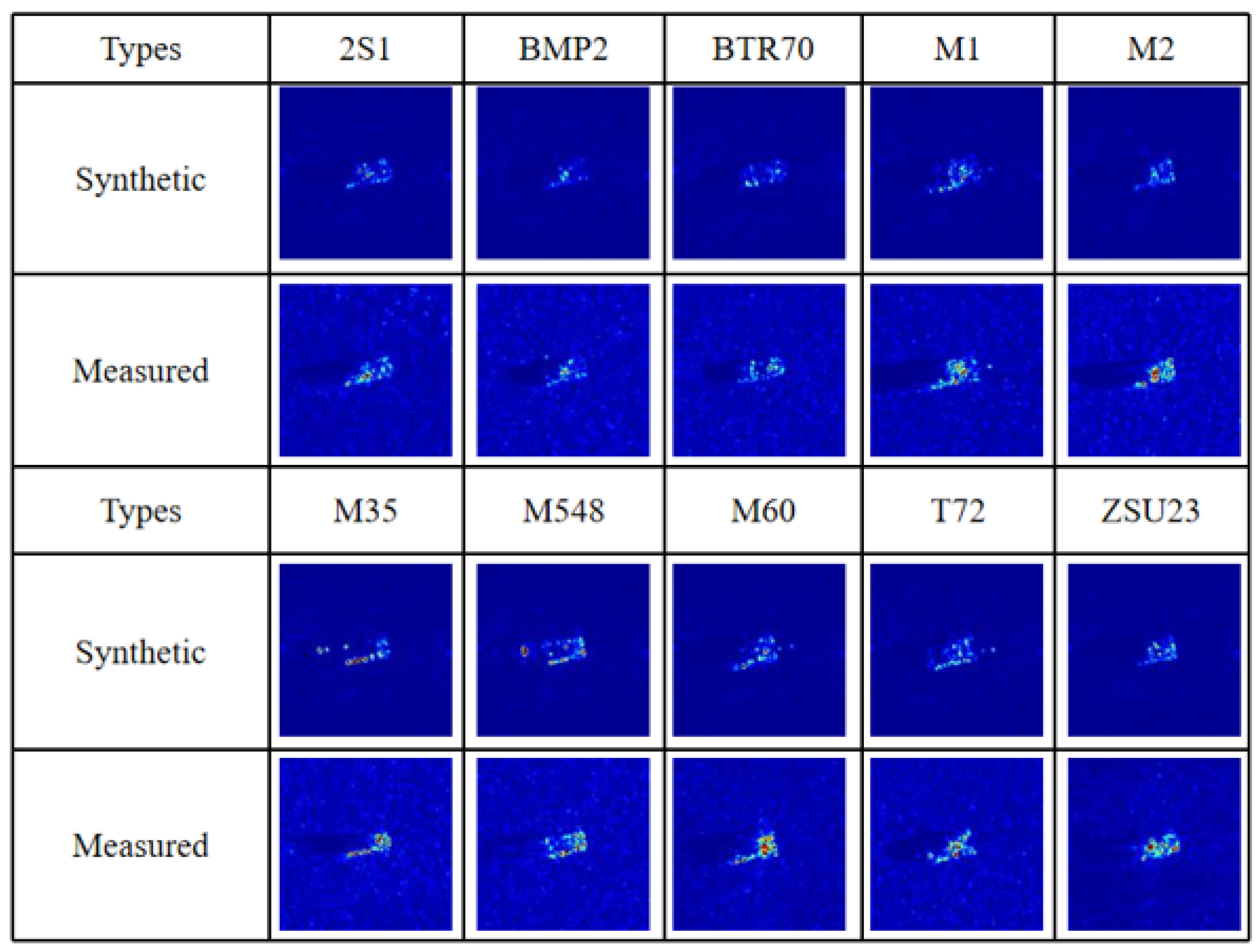
Figure 7 shows one (measured, synthetic) pair from each type. We can clearly see that the synthetic images lack background clutter, which is also mentioned in the literature [23,24]. Additionally, the strong scattering centers are somewhat different for the synthetic and measured data.

We also consider the experimental setting in Ref. [25] in our paper. The depression angles of the synthetic data range from 14 to 16 and the depression angle of the measured data is 17. Compared with “Training Scenario I”, there is a difference in depression angle for synthetic and measured data.

Table 2. Training Scenario II: data types and numbers of samples for training and testing in [25].

		Synthetic (Training)	Measured (Testing)
	Depression Angles	14°–16°	17°
Types
2S1		116	58
BMP2		55	52
BTR70		43	49
M1		78	51
M2		75	53
M35		76	53
M548		75	53
M60		116	60
T72		56	52
ZSU23		116	58
Total		806	539

shows the specific data types and numbers of samples for training and testing, and this experimental setting is called “Training Scenario II”.

The software and hardware environment of the experimental model training and testing is Intel(R) Xeon(R) CPU E5-2643 v4 @3.40 GHz, 128 GB memory, Nvidia GeForce GTX 1080ti with 11G RAM. The operating system is Ubuntu 16.04.1 and the development environment is Python 2.7.12 and TensorFlow 1.8.0.

Our work explores the problem of training fully on the synthetic data and testing on the measured data. Therefore, training data refers to synthetic data and test data refers to measured data. We explore the effectiveness of our framework under two training scenarios. In the following experiments:

(1)

for the image preprocessing, we crop the data to the size of 64 × 64 to exclude the influence of the background, and then we normalize them by min-max scaling to the range [0, 255].

(2)

for the network parameters, we use the grid search [61] method to explore the parameters. We provide a list of candidate values for the key parameters, and their final values are determined through experiments. The final parameter combination has a batch size value of 256, a dropout value of 0.2, and a $\lambda$ value of 10. We set the total epoch number to 500. We use the Adam [62] optimizer with a learning rate of ${10}^{-4}$.

(3)

as for the presented experimental results, we carry out each group of experiments by 20 times, and we also provide the lowest and highest recognition rates, represented by “Min” and “Max”, respectively. “Ave” provides the average recognition rates of 20 experiments with the standard deviation.

4.2. Recognition Results of Basic Recognition Network

We perform the experiments that utilize the basic recognition network introduced in Section 3.1 for the two training scenarios without feature alignment and self-training.

Table 3. Recognition results under different training scenarios (%).

Training Scenarios	Min	Max	Ave
Training Scenario I	77.84	81.78	79.83 ± 1.23
Training Scenario II	75.70	81.82	79.32 ± 1.79

shows the experimental results. Furthermore, to check the convergence property of our designed basic recognition network structure under two training scenarios, the curves of the loss value versus the number of epochs are shown in Figure 8, and the epoch number is set to 200 when training the basic recognition network.

When we carry out the experiments under Training Scenario II, the average recognition results are lower and display more apparent fluctuation. As mentioned before, the training and test data of Training Scenario I are paired, and the quantities of training data and test data under Training Scenario I are larger. Thus, it is not suitable to directly compare the recognition results of these two recognition scenarios. As shown in Figure 8, the curve of Figure 8a is smoother, and there is almost no oscillation compared to Figure 8b, and the difference to obtain Figure 8a,b is the training data, which also illustrates that Training Scenario II is more complicated. Nevertheless, the final convergence values of Figure 8a,b are similar, and the experimental results are similar under both training scenarios. The following validation experiments are carried out under Training Scenario II since the experiments are faster with a smaller amount of training data.

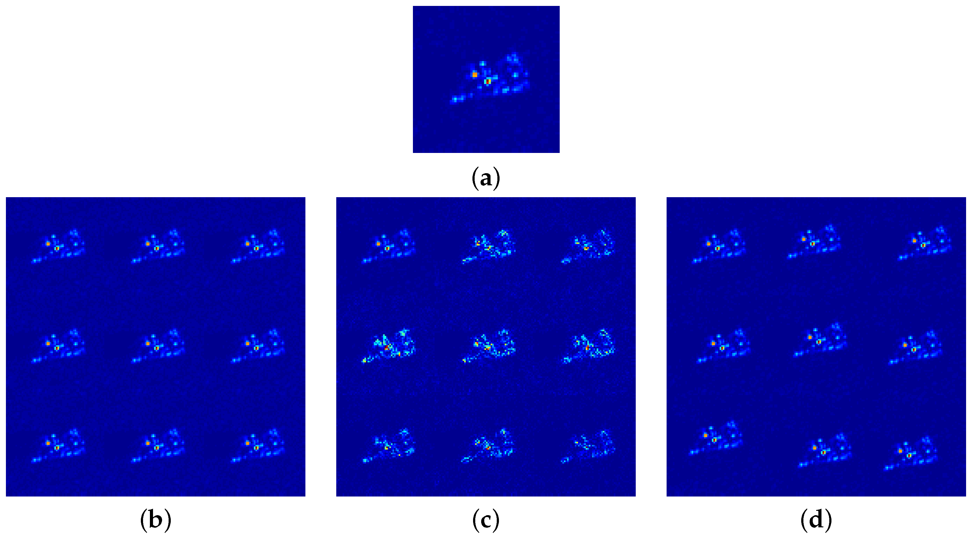
Then, we observe the experimental results under different data augmentation methods, namely by adding Gaussian noise [25], speckled noise [7], and translational augmentation [6,7]. Adding noise may address the distribution gap problem because the synthetic data lack background clutter.

In Ref. [25], to add Gaussian noise $\mathcal{N}$ to a training image x, a standard deviation (std) $\alpha$ is set, and the augmented image can be expressed as $x_{gaus}=x+\mathcal{N}$ (mean = 0, std = $\alpha$). In our paper, we set the $\alpha$ range as $\alpha =[0.1,0.2,0.3,0.3,0.4,0.4,0.5,0.5,0.6]$, and thus the training data is augmented by 9 times. In Ref. [7], to apply speckle noise to a training image x, the truncated exponential distribution s, which imposes that the maximum intensity of noise samples does not exceed a given parameter a, is used, and the augmented image can be expressed as $x_{spec}=\tilde{x}\times s$. $\tilde{x}$ is the image after applying a median filter on the x. The a range is set as $a=[0.5,0.5,0.5,1.0,1.0,1.0,1.5,1.5,1.5]$, and thus the training data is also augmented by 9 times. For translational augmentation, given a training image x, the translated image $x^{\prime }$ can be written as $x^{\prime }=x_{u,v}$, which illustrates that all pixels in x are shifted left by u pixels and shifted down by v pixels. $x^{\prime }$ has the same size as x. To guarantee that the target does not exceed the image boundary, the absolute values of u and v are smaller than 20. Figure 9 gives an illustration of the three data augmentation operations.

We also conduct the experiments on the basic recognition network introduced in Section 3.1 under Training Scenario II, and we augment the training data using the three data augmentation methods.

Table 4. Training Scenario II: recognition results of different data augmentation methods (%).

Augmentation Methods	Min	Max	Ave
Without augmentation	75.70	81.82	79.32 ± 1.79
Gaussian noise	76.62	84.60	81.36 ± 2.09
Speckle noise	79.78	86.27	82.29 ± 1.89
Translation augmentation	61.97	71.61	66.53 ± 2.63

provides the recognition results.

Speckle and Gaussian noise augmentation are both helpful for improving recognition rates. The improvement in recognition performance after adding speckle noise is better than after adding Gaussian noise, with a higher average recognition rate and a minor standard deviation. The literature [63] also mentions that adding speckle noise for augmentation is more effective than adding Gaussian noise. Moreover, we can see that translational augmentation does not help to improve recognition accuracy. The literature [25] also considers rotation augmentation; however, the experimental results show that rotation augmentation is not helpful for improving recognition performance [25]. This type of augmentation method, which includes translation, rotation, or their combination, may not be suitable in this scenario, and may even lead to an overfitting problem with unsatisfactory results.

Therefore, we consider using speckle noise augmentation in our following experiments, which provides better results.

4.3. Results of Gradual Domain Adaptation Recognition Framework

This subsection discusses the recognition results of our proposed gradual domain adaptation recognition framework. It is worth mentioning that pseudo-label denoising is not carried out in this subsection. Because the gradual domain adaptation recognition framework is a two-stage training process, we discuss the effectiveness of both the feature alignment and self-training, represented by “feature alignment” and “self-training”, respectively. “Baseline” gives the result of the basic recognition network introduced in Section 3.1 with speckle noise augmentation of the training data.

Table 5. Training Scenario I: recognition results in different stages of gradual domain adaptation recognition framework (%).

Methods	Min	Max	Ave
Baseline	78.07	85.80	81.57 ± 2.19
Baseline + feature alignment	91.00	94.42	92.65 ± 1.11
Baseline + feature alignment + self-training	92.05	96.73	94.94 ± 1.46

and

Table 6. Training Scenario II: recognition results in different stages of gradual domain adaptation recognition framework (%).

Methods	Min	Max	Ave
Baseline	79.78	85.16	82.29 ± 1.89
Baseline + feature alignment	88.68	92.58	90.09 ± 1.10
Baseline + feature alignment + self-training	92.76	98.70	95.71 ± 1.93

show the experiment results under Training scenarios I and II, respectively.

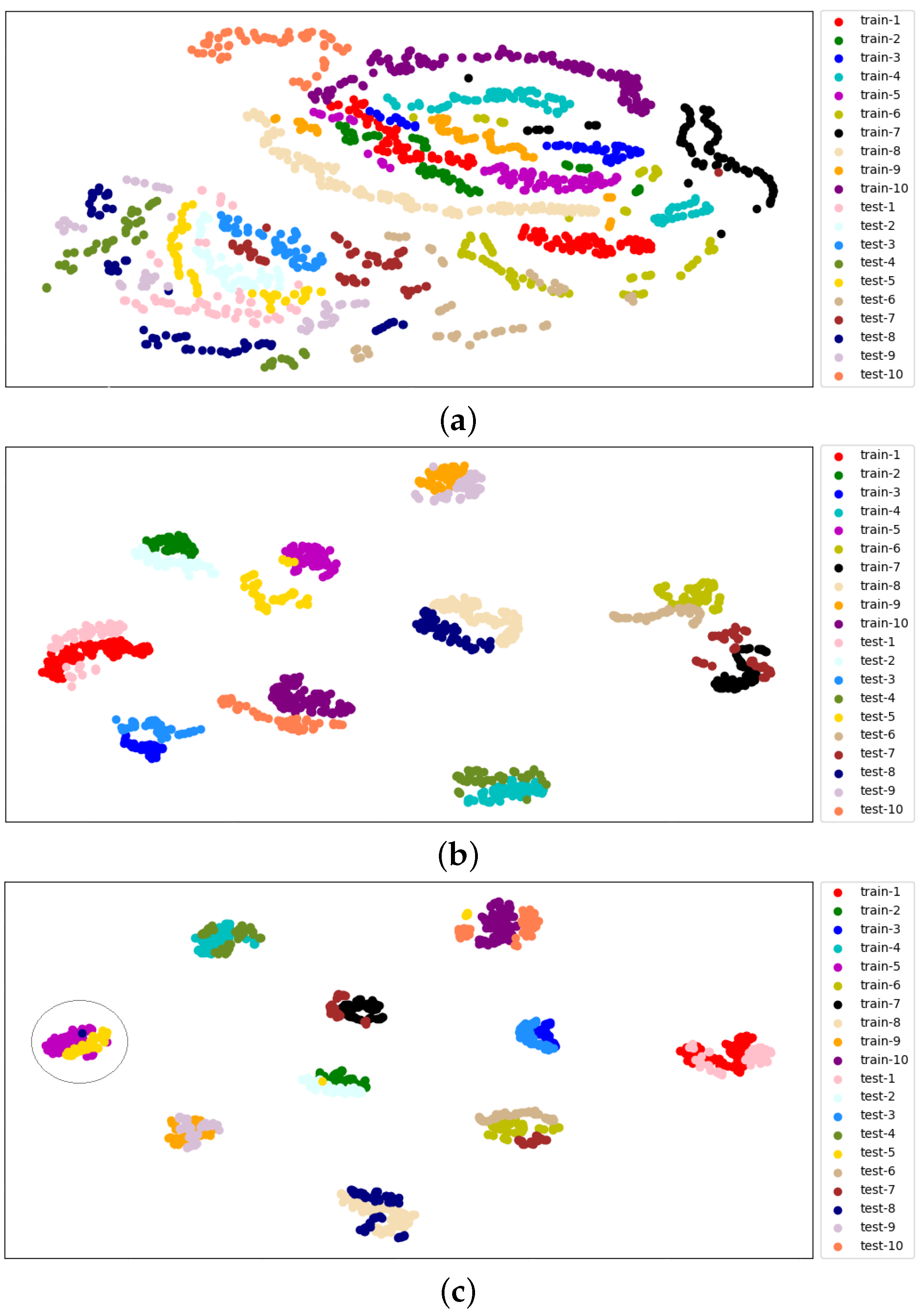
Table 5 and Table 6 show that the proposed gradual domain adaptation recognition framework is applicable under Training scenarios I and II settings. Furthermore, the recognition results show incremental improvements. We use the t-distributed stochastic neighbor embedding (t-SNE) [64] method, which can visualize high-dimensional data by mapping them into low-dimensional space, to further illustrate the effectiveness of our framework and compare the feature distributions extracted by the gradual domain adaptation classification network. We map the original vectorized images and features into a 2D space, and Figure 10 shows the visualization results.

The t-SNE visualization results also illustrate that our proposed gradual domain adaptation framework is effective. Figure 10a shows that there is a distribution gap between the original measured and synthetic data. Most of the training data are already distinguishable after the feature alignment classification, as shown in Figure 10b. However, some categories are not well separated, and the feature distribution of some categories is not compact enough. As shown in Figure 10c, after feature alignment and self-training, the feature distribution of different categories is more compact than we expect. Still, we can see that some samples are in the clusters of other classes (a sample of the test-8 category is in the train-5 cluster, which is shown in the grey circle of Figure 10c).

Thus, in the following subsection, pseudo-label denoising is considered in the self-training process for a better recognition result.

4.4. Effectiveness of Pseudo-Label Denoising Method

We performed pseudo-label denoising in the self-training process. In this subsection, we use three similarity measures, namely COSS, NMIS, and SSIM, for pseudo-label denoising according to Algorithm 1.

Table 7. Training Scenario I: recognition results of gradual domain adaptation recognition framework with pseudo-label denoising using different similarities (%).

Similarity	Min	Max	Ave
COSS	94.28	97.92	96.25 ± 0.78
NMIS	92.93	96.95	95.69 ± 1.30
SSIM	92.04	99.18	96.46 ± 1.14

and

Table 8. Training Scenario II: recognition results of gradual domain adaptation recognition framework with pseudo-label denoising using different similarities (%).

Similarity	Min	Max	Ave
COSS	92.57	100	96.59 ± 2.36
NMIS	91.84	100	96.87 ± 2.20
SSIM	95.73	98.70	97.36 ± 0.87

show the experimental results of the gradual domain adaptation recognition framework with pseudo-label denoising under Training scenarios I and II, respectively.

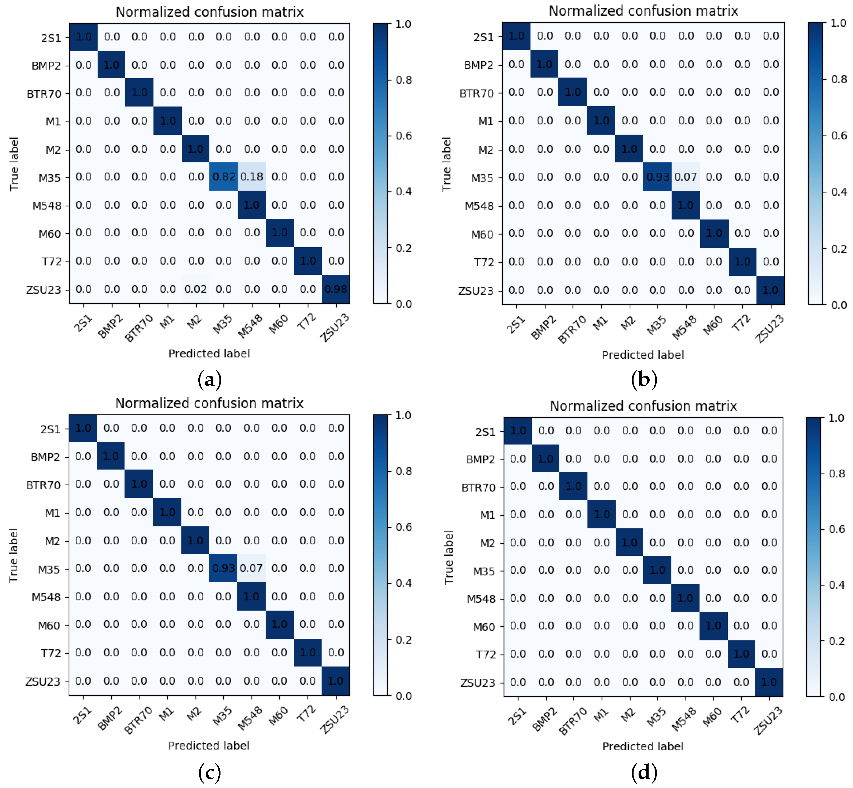
Using different similarity measures for pseudo-label denoising is helpful for improvements in recognition performance. SSIM performs better with higher average recognition rates in Training scenarios I and II. Here, we also present the confusion matrices of the pseudo-labeled dataset before and after denoising to illustrate the effectiveness of pseudo-label denoising, which are shown in Figure 11.

We can see that in the pseudo-labeled dataset without denoising, there are some mispredicted samples obtained by the feature alignment classification network. Figure 11b–d show that after the pseudo-label denoising, the correctness of the pseudo-labeled data has improved, and all the false pseudo-labeled data are eliminated when using the SSIM similarity for denoising. Mispredicted pseudo-labeled samples are the main factors that affect the further improvement of recognition rates, and label denoising can improve recognition performance. These results are also consistent with the experimental results in Table 7 and Table 8, which illustrate that SSIM performs better. Furthermore, in the following experiments, the final results are shown using pseudo-label denoising using SSIM.

4.5. Comparisons with Other Methods

In this subsection, we compare our framework with other existing methods using the SAMPLE dataset under the two experimental settings, given in

Table 9. Training Scenario I: comparisons with other methods (%).

Methods	Min	Max	Ave
Lewis et al. (2019) [65]	-	84.8	82.05
Araujo et al. (2022) [32]	-	-	91.3
Dong et al. (2021) [30]	-	-	93.66
Melzer et al. (2021) [31]	96.88	96.88	96.88
Our framework	92.04	99.18	96.46 ± 1.14

and

Table 10. Training Scenario II: comparisons with other methods (%).

Methods	Min	Max	Ave
Lewis et al. (2019) [24]	-	-	24.97
Scarnati et al. (2019) [23]	-	-	55.62 ${}^1$
Inkawhich et al. (2021) [25]	93.32	96.66	95.06 ± 0.87
Our framework	95.73	98.70	97.36 ± 0.87

¹ The exact recognition result of [23] is not presented in the original paper. We refer to [32] and give the experimental result here.

, respectively. More experimental results of different CNN architectures can be found in [25,31], and we only present the best recognition results achieved in [25,31] as the comparison.

Currently, more studies are carried out under Training Scenario I, and the best recognition accuracy is achieved by neural architecture searching [31]. However, neural architecture searching is computationally expensive and usually difficult to achieve in real-world systems. The recognition results of our framework under Training Scenario I reach a relatively high level of accuracy. In addition, under Training Scenario II, our framework exceeds the results presented in the literature [25], which utilized an ensemble of five models. Other research works use the SAMPLE dataset for recognition with different experimental settings. For example, in Ref. [29], except for the labeled synthetic data, one or two measured samples per class are also used for training, and their proposed augmentation technique can achieve 95.1% classification accuracy, and our experimental results still outperform it. Thus, our proposed method has achieved the state-of-the-art level.

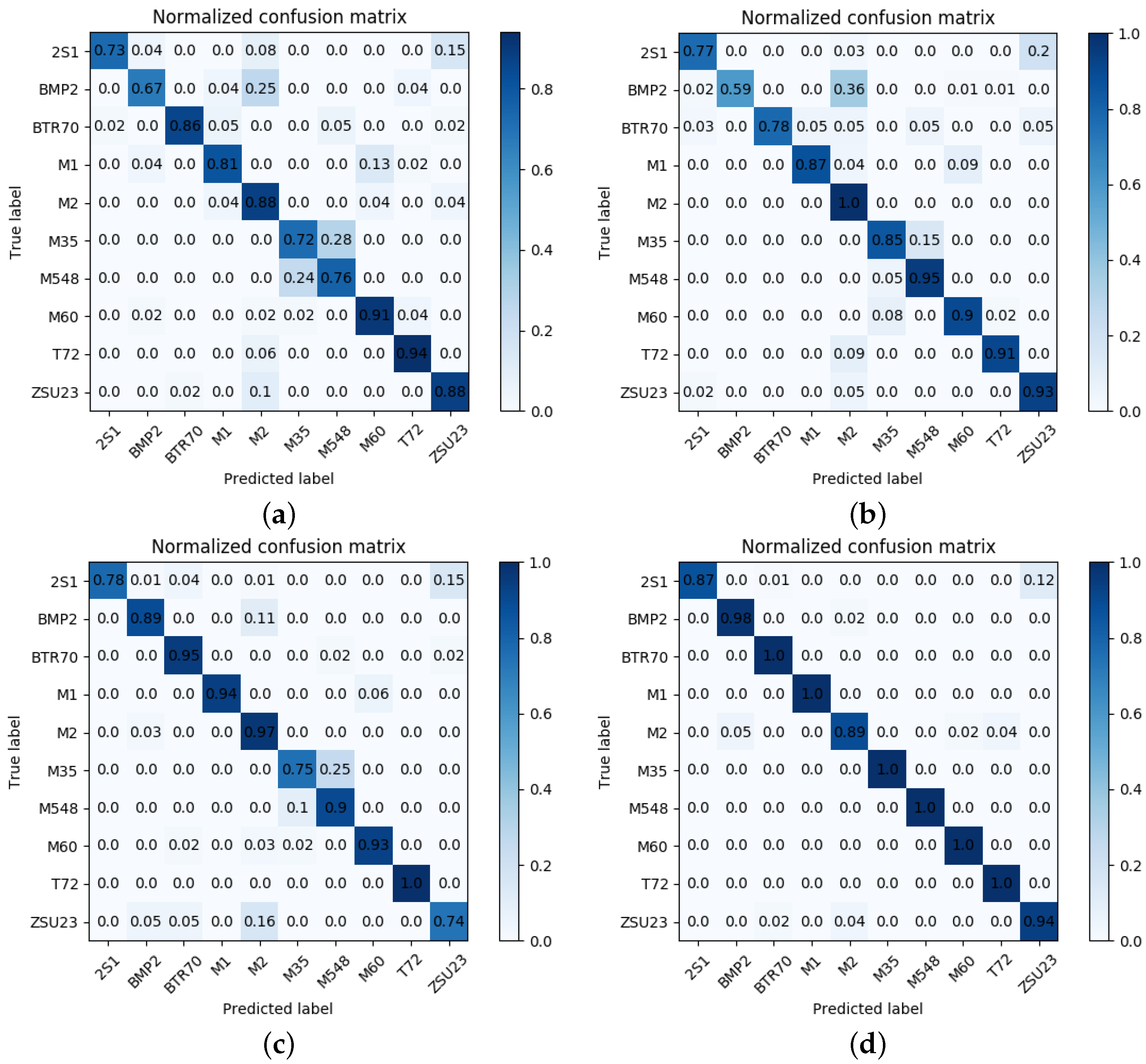
We further illustrate the effectiveness of the whole framework through the confusion matrices of the test data in Figure 12, which are obtained at different training stages under Training Scenario II. Figure 12a,b gives the results of the basic recognition network with or without data augmentation operation. Figure 12c gives the result of the feature alignment classification network with speckle noise augmentation. Moreover, Figure 12d gives the final result of the whole framework with pseudo-label denoising.

Firstly, we can see that the recognition results are progressively better. Secondly, as seen in Figure 12a–c, the M35, 2S1, and M548 categories are hard to recognize. Thirdly, comparing Figure 12b,c, feature alignment may cause the features of M35 and M548 to become closer. Fourthly, comparing Figure 12c,d, we can see that the denoised pseudo-labeled dataset improves the recognition results effectively. Therefore, all the methods of our framework work together to obtain the final results.

4.6. Ablation Analysis of Our Proposed Method

Because our overall framework combines many different kinds of methods, such as data augmentation, feature alignment between domains, self-training, and the pseudo-label denoising method, we consider the ablation experiments in this subsection to verify the effectiveness of these methods (

Table 11. Ablation analysis (%).

Speckle Noise Augmentation	Feature Alignment	Self-Training	Pseudo-Label Denoising	Ave
✔				82.29 ± 1.89
	✔			82.52 ± 1.22
		✔		87.87 ± 2.37
✔	✔			90.09 ± 1.10
✔		✔		82.81 ± 2.85
	✔	✔		86.60 ± 4.06
✔	✔	✔		95.71 ± 1.93
✔	✔	✔	✔	97.36 ± 0.87

). We perform the ablation analysis under Training Scenario II.

By ablation analysis, we can observe that when any method of our designed framework is removed, the performance degrades, verifying that (1) these methods, which are speckle noise augmentation, feature alignment, and self-training are all effective for improving the performance; (2) the utilization of self-training usually leads to a higher standard deviation since the effectiveness of self-training methods mainly depends on the initially trained classifier and the size of the original training dataset, and the larger size of the original dataset makes the pseudo-labeled test data a smaller proportion in the fine-tuning process. Thus, we use the feature alignment classification network obtained by the speckle noise augmented training data, which can provide more stable classification performance; (3) pseudo-label denoising scheme can lead to a better result, with a higher and more stable recognition rate. We can see that the whole framework works together to obtain the final result.

5. Discussion

We also discuss some limitations of the proposed method here. For the problem of training fully on the synthetic data and testing on the measured data considered in this paper, we need to know the categories of synthetic and real data in advance. However, in the real-world recognition scenario, it may be difficult to know the categories of real data in advance. Considering the proposed framework, self-training is a crucial step in our proposed framework, and it relies on the initially trained classifier. We have tried different basic recognition network structures, based on which the proposed feature alignment and self-training with pseudo-label denoising strategies can also improve recognition performance, but the final experimental results are not so good. Therefore, we proposed a feature alignment classification network for a better-initialized recognition result and a pseudo-label denoising method to eliminate the falsely pseudo-labeled data. In addition, there is still room for improving the pseudo-label denoising method, and some pre-set parameters are manually designed, which can be optimized. As a whole, seen from the experimental results, the proposed gradual domain adaptation framework has indeed achieved incremental improvements.

6. Conclusions

In our paper, we design a gradual domain adaptation recognition framework with a pseudo-label denoising method when using only synthetic data for training. The experiments are carried out based on the newly published SAMPLE dataset. Two training scenarios are considered to eliminate the controversy over the completeness of the experimental dataset. The experimental results demonstrate the effectiveness of our framework. For Training Scenario I, the framework matches the result of neural architecture searching and achieves 96.46% average accuracy. For Training Scenario II, the framework outperforms the results of other existing methods and achieves 97.36% average accuracy. Moreover, pseudo-label denoising effectively reduces the fluctuation of experimental results to gain more stable results. In the future, when training fully on the synthetic SAR data and testing on the real SAR data, more complex recognition scenarios can be considered, for example, reducing the amount of training data. We will evaluate the performance of our proposed method based on other SAR datasets and consider further improving the stableness of recognition results. While the pseudo-label denoising method can also be optimized and more similarity measures or combinations can be considered for pseudo-label denoising. To conclude, the recognition methods when training fully on the synthetic SAR data and testing on the real SAR data are worth further exploration. In the real-world recognition system, the real SAR data is demanding to obtain, and it has the application potential to utilize synthetic data for recognition.