Abstract
The definition of strategies for forest restoration projects depends on information of the successional stage of the area to be restored. Usually, classification of the successional stage is carried out in the field using forest inventory campaigns. However, these campaigns are costly, time-consuming, and limited in terms of spatial coverage. Currently, forest inventories are being improved using 3D data obtained from remote sensing. The objective of this work was to estimate several parameters of interest for the classification of the successional stages of secondary vegetation areas using 3D digital aerial photogrammetry (DAP) data obtained from unmanned aerial vehicles (UAVs). A cost analysis was also carried out considering the costs of equipment and data collection, processing, and analysis. The study was carried out in southeastern Brazil in areas covered by secondary Atlantic Forest. Regression models were fit to estimate total height (h), diameter at breast height (dbh), and basal area (ba) of trees in 40 field inventory plots (0.09 ha each). The models were fit using traditional metrics based on heights derived from DAP and a portable laser scanner (PLS). The prediction models based on DAP data yielded a performance similar to models fit with LiDAR, with values of R² ranging from 88.3% to 94.0% and RMSE between 11.1% and 28.5%. Successional stage maps produced by DAP were compatible with the successional classes estimated in the 40 field plots. The results show that UAV photogrammetry metrics can be used to estimate h, dbh, and ba of secondary vegetation with an accuracy similar to that obtained from LiDAR. In addition to presenting the lowest cost, the estimates derived from DAP allowed for the classification of successional stages in the analyzed secondary forest areas.
Keywords:
enhanced forest inventory; DAP; LiDAR SLAM; cost analysis; classification; atlantic forest 1. Introduction
In different regions of the planet, the extreme effects of climate change (e.g., high air temperature, floods, long periods of drought, forest fires, and so on) are increasingly present. As a result of these effects, researchers from different areas have expressed concerns about current and future climate conditions and their possible impacts on the maintenance and conservation of life on Earth. The current model of economic and social development adopted by large nations has been criticized as the main culprit of climate change. This unsustainable model has caused considerable changes to the ecological balance and biodiversity of the planet due to significant deforestation and forest degradation in various ecosystems [1,2,3,4,5,6].
As such, methods of estimating deforestation and vegetation degradation are increasingly needed at different spatial scales, with low cost and short time intervals [7]. To ensure that the ecosystem is ecologically balanced, it is necessary to know the characteristics of each type of environment in order to identify strategies to maintain, preserve, or recover healthy conditions. One of the most efficient ways to identify the successional stages of a given forest is by quantifying what exists in the vegetation of interest, which can be achieved by carrying out forest inventories. Research has indicated that accurate forest inventories increase the reliability of decision-making in forest management [8,9,10].
For sustainable management, it is necessary to obtain accurate information on the composition and structure of forests. Forest inventories become essential in providing this information. However, in order to obtain a high level of confidence in the information collected, it is necessary to measure the population under study in a representative way. However, with current methods, the more representative the sample is, the higher the costs are to obtain it. This paradox between cost and precision is one of the great research dilemmas for traditional forest inventories (TFIs). Traditional methods imply the use of fixed area plots, in which the diameter and total height of all trees within the plot are measured, in the case of natural forests, which also requires the identification of species and, in some situations, the measurement of other variables of interest [11,12].
Comparatively, TFIs are much more costly in native forests than in planted forests due to difficulties with accessibility, allocation of plots, movement within the forest, and the greater number of variables to consider. In addition, these TFIs require a greater amount of human resources and have many operational risks as well as limited spatial coverage. Thus, current demands for information exceed the scope of many methods of TFIs, especially in natural forest formations [13,14].
Remote sensing techniques offer an effective and less costly alternative to the quantification of forest parameters [15]. In this context, three-dimensional vegetation formations collected by light detection and ranging (LiDAR) and digital aerial photogrammetry (DAP) using unmanned aerial vehicles (UAVs) have been successfully used to improve traditional inventories [10]. Despite the ability of the LiDAR data to represent the vertical structure of the vegetation and the terrain where it is located, its cost can still be considered high, especially in developing countries. In contrast, the information obtained via DAP-UAVs generally presents a lower cost and may therefore be a viable alternative. Although the difficulty of DAP in representing understory and land under the forest can be considered a limitation, multiple studies have demonstrated its solid performance in estimating characteristics of forest interest [16].
Identifying and understanding the ecological relationships within the different successional stages is fundamental for the maintenance of those ecological values that still exist as well as for the identification of strategies to recover degraded areas. In general, methods for classifying forest ecological succession are based on aspects of vegetation organization [17,18], with emphasis on abundance (i.e., horizontal structure), size (i.e., vertical structure), and composition (i.e., species diversity). To ensure sustainable forest management, successional stage classification must cover large areas with vegetation. However, classification methods are normally based on field data collected in forest inventory campaigns. While these field-based classifications are accurate, they are also spatially limited and representative only of inventoried plots [19].
Succession is a three-dimensional process, and some types of remote sensing data (i.e., LiDAR, SAR, and DAP) are sensitive to the three-dimensional structure of the vegetation canopy and can therefore provide accurate estimates of vegetation structure (mainly vertical) [20,21]. Thus, unlike methods based on field data, this makes it possible to classify the successional stage of large areas of forest. Nonetheless, studies that use DAP-UAV data to classify the successional stages of different types of forest formations around the world remain rare.
The Atlantic Forest biome possesses great importance due to its high biodiversity and size. It is currently considered one of the richest ecosystems on the planet in terms of biological diversity. The biome is a hotspot, but it continues to suffer from numerous anthropic pressures. Its vegetation cover reached 28%, in which the remainder is distributed in fragments of up to 50 hectares [22,23]. Because it is an ecosystem composed of native forest settlements, the need for detailed, accurate forest inventories within the shortest possible time spaces are essential for good management of this natural resource.
Based on the above points, this study evaluated the potential of low-cost 3D DAP-UAV point cloud data to classify the successional stage of different areas of a tropical secondary Atlantic Forest in Brazil.
2. Materials and Methods
2.1. Study Area
The study was carried out in eight areas in the Atlantic Forest biome, located in the north of the state of Espírito Santo, Brazil (Figure 1). According to the Köppen–Geiger classification, the region has a predominantly “Aw” climate, meaning that it is rainy and tropical with a dry season in winter. It has an average annual temperature of 23.6 °C and average annual precipitation of 1.290 mm. Geographically, the area is predominantly flat relief (80%), with a lower proportion of bumpy relief (19%) and an average altitude of 55 m. The soil of the region is classified as dystrophic yellow argisol [24,25,26]. The eight areas studied comprised approximately 201 ha.
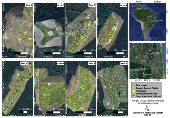
Figure 1.
Location of the study area and their field plots.
2.2. Methods
To evaluate the use of DAP-UAV as a tool for forest inventories to classify Atlantic Forest succession stages and to compare it with LiDAR PLS in terms of accuracy and costs, structured steps were followed (see Figure 2). To begin (step 1), the criteria for the classification of succession stages were defined based on the national council for the environment (CONAMA) resolution 29/94 (http://conama.mma.gov.br) [27]. In step 2, a field inventory was carried out using the traditional method seeking to cover the greatest possible vegetation variation. Thus, height (h), diameter at 1.30 m from soil level (dbh), and basal area (ba) were measured in 40 fixed area plots of 0.09 ha that ranged from clean pasture to the advanced stage of succession. Later (step 3), 3D point clouds were generated via DAP-UAV and LiDAR PLS in the same plots. In step 4, regression models were adjusted and validated to estimate the values of h, mean dbh, and ba from the traditional metrics based on the heights of the DAP and LiDAR point cloud. The accuracy of the two methods was compared using the RMSE and R² of the models. In step 5, maps of vegetation successional stage were generated with a spatial resolution of 30 m through application of the models obtained for DAP-UAV and the pre-established intervals of h, mean dbh, and ba, as per CONAMA resolution 29/94 [27]. Finally (step 6), a comparison was made of inventory costs using the traditional method and the method using LiDAR PLS and DAP-UAV.
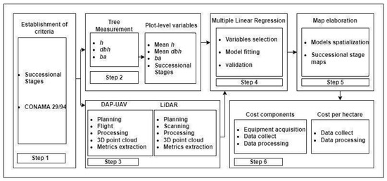
Figure 2.
Flow of structured steps to perform the work.
2.2.1. Traditional Forest Inventory
Data from the traditional forest inventory method were collected in two campaigns, the first between 25 July and 30 July 2021, and the second between 13 September and 25 September 2021. Forty permanent quadrangular plots (30 × 30 m) were randomly allocated, with a total area of 3.6 ha (Figure 1). The area of the plots (0.09 ha) sought to reduce possible effects of clearings and very large trees in the extrapolation of data. The plots were located primarily in places with flat relief and respected (when possible) a minimum distance of 25 m from the edges of the vegetation and of at least 50 m between plots. The plots were oriented towards magnetic north by using a compass, and their vertices were marked with piles with the aid of surveyor and tape measure squares and were georeferenced with precision RTK using the SIRGAS 2000 UTM 24 S Reference Coordinate System (SRC). Average RMSE values at x and y coordinates were 0.34 m.
Data collections were always initiated by vertex A, which was always southwest (SW). The other vertices (B, C, and D) were marked clockwise and followed alphabetical order. All adult arboreal individuals with living stems and dbh greater than or equal to 5 cm were measured at 1.30 m from the ground, with the bases of their trunks completely within the limit of the plot. Every tree measured was identified via sequential numbering within the plot. Trees with more than one stem out below 1.30 m were considered multi-stem and had all spleens with the minimum inclusion diameter measured and identified using the same number followed by an alphabetic differentiator (e.g., 1a, 1b, 1c… 1n). The h of the trees, corresponding to the length between the base of the trunk and the apex of the canopy, was measured with the aid of a graduated ruler of 15 m. For the measurement of trees in which the height exceeded the limit of the ruler, the Suunto PM-5/360PC Clinometer (https://www.suunto.com, accessed on 27 October 2022) [28] was used. This instrument is based on trigonometric principles, so it is essential to know the distance between the observer and the tree so that the readings (lower and upper) are correct. In addition, it is necessary to consider the topography of the site [29]. In this case, the distance between the observer and the trees varied according to the specificity of each individual tree, with the aim of finding the best position to measure each tree. Equation (1) was used to obtain the total tree heights.
Here, h is the total height; α and β are the lower and upper angles, respectively; and L is the distance between the observer and the tree.
2.2.2. Classification of the Successional Stage
Initially, the study areas were chosen from pre-existing maps provided by the company that owns the areas. These maps used six vegetation classes that were characterized based on visual criteria. These classes are presented in Table 1 and were used to facilitate the distribution of TFI plots in order to cover the greatest possible vegetation variation. Therefore, five plots were used in each of these classes by the company that owns the area.

Table 1.
Classes of vegetation used for the distribution of plots and number of plots sampled.
After the TFI, the plots were reclassified according to the criteria defined in CONAMA resolution 29/94 [27] (Table 2). For a plot to be classified as belonging to a given stage, it was established that it must present at least two parameters framed in the stage in question. It is important to note that the criteria established by CONAMA [27] have overlap bands between the stages, with the possibility of the same area falling into two stages. In this case, the area in question is considered in transition between the initial and middle stages or the middle and advanced stages.
Table 2.
Criteria for classification of succession stages of the studied areas.
2.2.3. Digital Aerial Photogrammetry (DAP)
UAV Photos
High-resolution spatial images were obtained by a DJI Mavic 2 PRO multirotor platform (SZ DJI Technology Co., Ltd., Shenzhen, China) between 21 September and 30 September 2021. The aircraft was equipped with an RGB camera with a 20-megapixel CMOS sensor and resolution of 5472 × 3648. The camera was installed in a gimbal to reduce possible mechanical vibrations at the time of taking the photos. The weather conditions included clear sky (<5% clouds) and wind speed of less than 10 m s−1 [30]. The flights were performed at a height of 120 m, respecting ICA 100–40 (https://publicacoes.decea.gov.br, accessed on 2 August 2022) [31] and used the visual line of sight (VLOS) method with longitudinal overlap of 75% and lateral overlap of 65%. The photos [32] were saved in .jpg format on a SanDisk 128GB Extreme microSDXC memory card. Approximately 201 ha were mapped with eight flights. The average time of each flight was approximately 10 min [33].
Structure from Motion Processing
The images obtained by UAV were processed using Agisoft Metashape software (http://www.foif.com) [34], which uses structure from motion (SfM) algorithms to perform image alignment and 3D point cloud generation. For the alignment of the photos and acquisition of the sparse cloud, the “high” precision and key point and mooring limits parameters of 40,000 and 10,000 points, respectively, were used. In the process of aligning the photos, ground control points (GCPs) were used. The GCPs were distributed within the flyover areas, with at least four GCPs per survey (Figure 1). The coordinates of the GCPs were collected using RTK with sub-metric precision using the SRC SIRGAS 2000 UTM 24 S. At the end of the alignment, the mean of the RMSE for the eight surveys was 0.55 m in X and Y and 0.95 m in Z. In the creation of the dense cloud of points, the parameters were defined as quality and “aggressive” depth filtering mode. The average ground sample distance (GSD) for the eight surveys was approximately 2.5 cm per pixel.
2.2.4. Light Detection and Ranging (LiDAR)
Data Collection
The plots were scanted using the LiDAR PLS GeoSLam ZEB-HORIZON 3D sensor, model GS_510254 (https://geoslam.com, accessed on 7 August 2022) [35], between 21 September and 29 September 2021. The five plots of the pasture class were not mapped due to the lack of trees. The weather conditions included clear sky (< 5% clouds) and wind speed of less than 10 m s−1. The ZEB-HORIZON is a 6.96 kg portable laser scanner (PLS) LiDAR model and consists of a 2D laser scanner with a wavelength of 903 nm. It features a motorized inertial measurement unit (IMU). The laser acquisition speed is 300,000 points per second, with a range of approximately 100 m around the equipment [35]. It has 16 sensors; a 270° × 360° field of view; vertical and horizontal angular vision of 2° and 0.38°, respectively; and relative accuracy up to ± 6 mm, depending on the environment. The geolocation of the clouds was subsequently adjusted in the GEOSLAM HUB software using the vertices’ stakes as a physical reference [36].
The scan was performed by an operator who held the equipment with his hands at a height of approximately 1.40 m from the ground while walking slowly (approximately 25 cm per second) throughout the interior in a zigzag, starting and ending at the “A” vertex of each plot (Figure 3). The mean scan time of each plot was approximately 5 min.
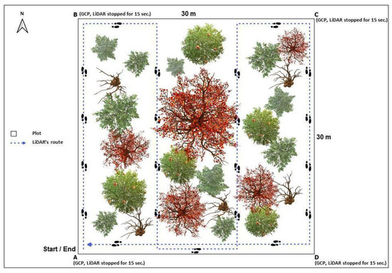
Figure 3.
Walking with LiDAR PLS inside the plot.
Pre-Elaboration of Point Clouds
The 3D point cloud was obtained from the raw data collected in the field and the GeoSLAM server. The application uses a [35] system based on Simultaneous Localization and Mapping (SLAM), which combines 2D laser scan data with IMU data to generate accurate 3D point clouds. Finally, 3D point clouds were produced for each of the plots, with an average density of approximately 800 points per square meter. The vertices of the inventory plots were used as GCPs to georeference the LiDAR point clouds. The coordinates of the four vertices of the inventory plots were collected with RTK, in UTM, SIRGAS 2000, 24 S.
2.2.5. Digital Terrain Model (DTM)
To obtain the digital terrain model (DTM), the 3D cloud points were first distinguished as ground points or not. The algorithm used for the classification of ground points was the “progressive morphological filter”, available in the LidR package [37] of the R software [38]. After the classification of the ground points, filtering was performed that kept only the soil points. Finally, the DTM was constructed from interpolation of the ground points by the inverse distance weighting (IDW) method, which is based on the assumption that the altitude value of an unsampled point can be approximated from the weighted average of the values of the sampled points within a certain distance (d) or a certain number of nearest neighbors (k).
2.2.6. Structural Metrics
Upon obtaining the DTM, normalization of the point clouds was performed; that is, the altitude of the DTM was subtracted from the elevation of the points of the cloud, allowing for the manipulation of 3D clouds as if they had been acquired on a flat surface and removing the influence of the terrain in the above-ground measurements [37]. After normalization of the point clouds, structural metrics were estimated based on information regarding the height of the points in the clouds using FUSION/LDV 3.42 software [39]. A threshold height of 1.5 m was used for the removal of soil points and separation of undergrowth [40]. The metrics were calculated from DAP, DAP-DTMLiDAR and LiDAR point clouds to describe the structure of each plot. The extracted metrics are described in Table 3.
Table 3.
Structural metrics extracted from point clouds derived from DAP-UAV, DAP-DTMLiDAR, and LiDAR PLS.
2.2.7. DAP-UAV Validation
The validation of DAP products was performed in two stages: (1) validation of the topographic products obtained (i.e., the DTM) and (2) validation of the data from the vertical structure of the normalized 3D point cloud.
DTM Validation
The altitude (Z) values of the vertices of the plots (160 points) collected in the field with the RTK were used to evaluate the accuracy of the DTM generated by the DAP. To evaluate the influence of vegetation on the representation of relief, vertices were classified as (i) with vegetation and (ii) without vegetation. Accuracy was evaluated using the values of RMSE and bias (absolute and percentage) and R² (Equations (2), (3), and (4), respectively).
Here, = observed dependent variable, = estimated dependent variable, = mean of the observed dependent variable, = mean of the estimated dependent variable, and n = number of observations.
Validation of the Vertical Structure of DAP-UAV Clouds
For validation of the vertical structure of the DAP and DAP-DTMLiDAR cloud, the maximum heights and dominant heights of the inventory and field plots were compared with the metrics “Hmax” and “HP95”, respectively, of the DAP point clouds of each plot. To determine the dominant heights of the plots, the average of 20% of the highest trees per hectare was used. For comparison purposes, the same analysis was performed with DAP-DTMLiDAR data. The Hmax and HP95 metrics of the point clouds were extracted using fusion/LDV 3.42 software and are respectively the highest point height value of the point cloud and the value of the height surpassing 95% of the points in the cloud. The statistics of RMSE and bias (absolute and percentage) and R² (Equations (2) and (3), respectively) were evaluated.
2.2.8. Estimated Models of Mean h, Average dbh, and ba
Multiple linear regression (MLR) models were adjusted to estimate the values of mean h, diameter, average dbh, and ba of trees at plot level. As predictor variables, the structural metrics extracted from the clouds of normalized points obtained by DAP, DAP-DTMLiDAR, and LiDAR were considered. The models adjusted for LiDAR and DAP-DTMLiDAR were used to compare the efficiency and quality of the models generated from DAP normalized clouds in terms of RMSE and R².
Pearson correlation analysis (Equation (5)) was performed to verify the collinearity between the variables. Multicollinear variables are considered when two or more predictors are related to each other and explain the dependent variable in a similar way. Non-multicollinear variables were considered as those that presented values within a threshold between −0.8 and 0.8. The multicollinearity analysis was performed before fitting of the models, maintaining only one predictor variable among each group of multicollinear variables.
Here, = Pearson linear correlation coefficient of the sample; = observed values for the variables , respectively; and
e
= average of the observed values in the variables , respectively.
The exhaustive search method was used with the aid of RStudio software and the Leaps package [41]. The exhaustive method tests and compares all independent variables (X) and finds the best subset to predict the dependent variable (Y) in linear regression by using the branch-and-bound algorithm. The independent variables were selected to adjust the models of each of the dependent variables in each of the datasets (DAP, LiDAR, and DAP-DTMLiDAR).
For each dependent variable in each dataset, subgroups were selected with one, two, three, four, or five independent variables. After selecting the predictor variables, the LMR models (Equation (6)) were adjusted.
Here, = value of the dependent variable in the i-th observation, corresponding to the mean h, mean dbh, and ba; β = model coefficients; X1i, X2i, … , Xpi are the values of the p-th independent variables in the i-th observation (data from the DAP, DAP-DTMLiDAR, or LiDAR point clouds); and εi = random error of the model.
For the choice of the best model for each dependent variable in each dataset, the RMSE and adjusted coefficient of determination (Equations (2) and (4)) were compared. For validation of the chosen models, the datasets were divided into 80% for fitting and 20% for validation with 1000 iterations. Subsequently, the frequencies of RMSE were compared.
2.2.9. Spatialization of DAP-UAV Models
With the DAP-UAV models adjusted for each vegetation variable, fusion/LDV 3.42 software was [39] used to obtain rasters where the pixel values correspond to the values obtained for each of the metrics used in the models. These rasters were obtained with a spatial resolution of 30 m × 30 m per pixel (same plot size) and afterwards were used in the application of the adjusted models to obtain the maps of h, dbh, and ba for each of the eight areas.
From the spatialization of the vegetation data, classification maps of the succession stages were created according to the criteria defined in Table 1. For this, the maps obtained for the estimation of h, dbh, and ba were used as input files following the flowchart presented in Figure 4. For a pixel to be sorted at a given stage, it must have at least two vegetation parameters framed in this class.
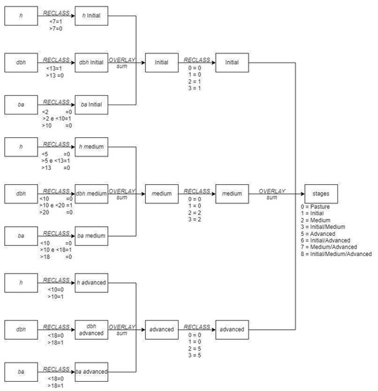
Figure 4.
Succession stage classification flowchart.
2.2.10. Cost–Benefit Analysis
In the cost–benefit analysis, the three methods of data collection were compared (i.e., DAP, LiDAR PLS, and TFI). To perform the analysis, three cost components associated with each method were analyzed, namely equipment (including software licenses), data acquisition, and data processing and analysis. First, the total costs of each method were calculated, and then the total costs of equipment acquisition as well as of data acquisition and analysis per hectare measured were separately identified. The costs were calculated with updated values for the month of June 2022.
For the DAP method, eight flights were performed that mapped a total area of 201 ha. For the areas measured by the TFI and PLS methods, the sum was found using the areas of the 40 plots of 0.09 ha, totaling 3.6 ha.
Regarding equipment costs, the costs of acquiring the equipment and software for each method were considered based on the use of a computer of the same model for each method. For the DAP and PLS methods, it was necessary to collect points with RTK, which required renting model equipment x for R$ 250.00/day. In total, 12 days were spent to collect 178 points, yielding a cost of R$ 16.85/point. Considering a daily 11 h workday, an average of 1.85 points/h were obtained per hour, which was used to calculate the cost of the hour/man to collect the points during data acquisition.
The costs associated with the data acquisition stage were calculated based on the time/man required for each step in each method, in addition to daily car rental and lodging. For the three methods, teams included three members. Hence, all hours/man were multiplied by three, with the exception of flight planning. Daily accommodation comprised a three-guest room. For accommodation and vehicle rental, the data collection days plus two nights for the team’s arrival and return were considered. For the collection of control points with RTK, an average of four GCPs was considered for each of the eight DAP flights, versus four GCPs per plot for PLS collections.
To evaluate the costs associated with the data processing and analysis component, the time/man required for each step in each of the methods was calculated. Only one person was considered for data analysis in the three methods.
The hour/man value was based on the technical time of R$ 153.00/hour for a professional agrarian scientist in the state of Espírito Santo [42]. It is necessary to emphasize that the data collections using the three methods were performed simultaneously in the same expedition for this study. Therefore, to calculate each method separately, the costs of the data acquisition, analysis, and processing components were diluted to the smallest unit of each item and evaluated based on how many units were required for each method.
3. Results and Discussion
3.1. TFI Results and Classification of Stage of Plots
The values of h, dbh, and ba, in addition to other parameters of the 40 plots of the TFI, are presented in Table 4 together with the classification of the succession stage of each plot according to the criteria defined by CONAMA 29/94 [27].
Table 4.
Parameters observed in TFI and classification according to CONAMA.
The plots in which the acronyms of the stages were added to the letter “E” indicate that infestation by invasive alien species was observed. The plots that did not meet the criteria of any of the three stages proposed by CONAMA Resolution 29/94 [27] were considered “Pasture”. Thus, the criteria established by CONAMA [27] do not always represent reality. For example, plots such as “32”, which according to what was observed in the field does not present pasture characteristics, have parameters that fall outside of the stages proposed by CONAMA [27]. Figure 5 shows the frequency of the main species found in each stage.
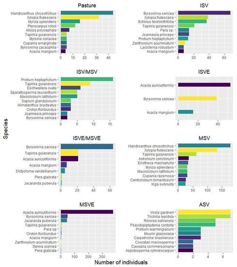
Figure 5.
Frequency of species by succession stage, according to the stages defined in Table 1.
3.2. Validation of DAP-UAV Data
3.2.1. Digital Terrain Model
Figure 6 presents the DTMs generated via DAP-UAV for each of the eight areas analyzed, in addition to the limit of inventory plots. The altitude values of the vertices of the plots collected in the field with the RTK varied between 2.5 and 41.7 m, while those estimated by the DAP varied between 3.7 and 47.8 m.
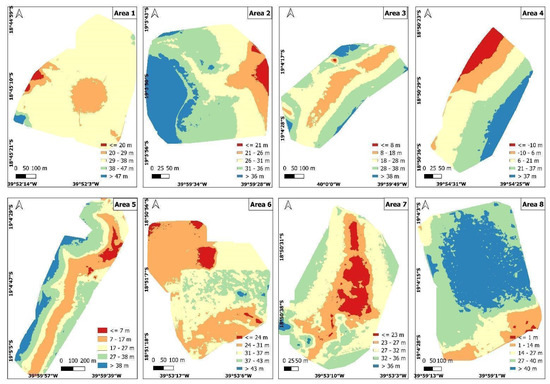
Figure 6.
Digital terrain models (DTMs) obtained with DAP-UAV data.
Table 5 assesses the accuracy of the elevation values estimated by DAP-UAV. Figure 7 displays the scatter plots between the measured and estimated altitude values of the terrain. A strong correlation (R² > 0.7) was observed between the values estimated by DAP and the values observed with RTK. The DAP was able to reconstruct with regular efficiency the soil position in areas that were fragmented or without vegetation (RMSE of 3.3 m, 15.6%, and R² of 0.87), underlining a greater difficulty in reconstructing the topography of the terrain in areas with denser vegetation (RMSE of 7.4 m, 38.1%, and R² of 0.80), as observed by Almeida et al. [40]. As forest cover becomes dense, the procedure of rebuilding the elevation of the terrain is more delicate and can prevent obtaining the altimetry points of the soil [32].
Table 5.
Statistics of the comparison between the altitude of the DTM generated by photogrammetry and the altitude of the terrain control points obtained by RTK in areas under vegetation (Present) and in areas without vegetation (Absent).
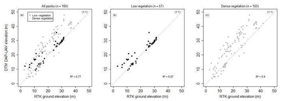
Figure 7.
Scatter plots between the altitude values of the DTM generated by photogrammetry and the altitude of the terrain control points obtained by RTK, where (a) represents all points, (b) represents points in places without vegetation, and (c) represents points in places under vegetation.
As observed in other studies, in general, the DAP also overestimated (n = 160; bias = −3.72 m, −18.60%) the elevation values, with a total error of 6.25 m (31.23%). The overestimation observed in this study may be related to DAP’s inability to penetrate the canopy and understory of vegetation. This limitation is even more evident when considering only the values of elevation of the terrain of the vertices of the plots under vegetation (n = 103), with R² of 0.8, RMSE of 38.13% (7.40 m), and bias of −26.16% (−5.07 m). At the vertices of plots without vegetation (n = 57), DAP’s capacity to reconstruct the land increases considerably, where RMSE = 15.6% (3.3 m), bias = −6% (−1.28 m), and R² = 0.87. Despite the better performance in points without the presence of vegetation, the values found in this study are lower than those observed in other studies. In addition to not being able to penetrate the forest canopy, DAP’s low ability to represent the terrain may be related to other factors, such as flight characteristics, the sensor used in taking the photographs, the SfM processing algorithm, or the physiographic characteristics of the area [10,40,43,44,45,46,47,48]. The algorithm used for sorting points representative of the terrain may also have been a source of error at the time of DTM generation [49,50].
Therefore, to survey fragments with extensive areas, it is recommended to perform flights that cover areas outside the fragment, seeking places where it is possible to visualize the terrain, such as roads or clearings, to improve representation of the altimetry of the terrain. The analysis presented concerns regarding the quality of the DTM in the evaluated points, and it is not possible to draw conclusions about the entire length of the area. To complement analysis of the accuracy of DTM and other products obtained by DAP, the maximum heights of the plots measured in the field were also compared with those estimated by DAP.
3.2.2. Heights of Trees
Maximum Height x Hmax
Table 6 presents the results of the accuracy analysis of the estimates of the maximum height of the trees per plot by DAP-UAV and DAP-DTMLiDAR. Figure 8 showcases the scatter plots for the maximum height values measured in the field and estimated (Hmax) by the two 3D point clouds. A clear correspondence can be noted between the Hmax values estimated by the DAP and DAP-DTMLiDAR point clouds, which have similar statistics (Table 6). Both 3D clouds underestimated (Table 6 and Figure 8) maximum height, a result that was expected and observed in other studies with the normalized point cloud of the DTM LiDAR [10]. In addition to the similarity between the estimates of maximum heights, the performance was also satisfactory, with RMSE and bias values below 18.21% and 0.71%, respectively. Almeida et al. [40] found an RMSE equal to 24% in a secondary Atlantic Forest in northeastern Brazil when estimating maximum heights.
Table 6.
Statistics of the comparison between the Hmax metric obtained by DAP-UAV and DAP-DTMLiDAR and the maximum heights of the plots obtained by the TFI.
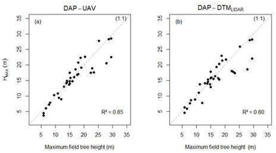
Figure 8.
Scatter plots between the Hmax metric obtained by (a) DAP-UAV and (b) DAP-DTMLiDAR compared with the maximum heights of the field plots.
Despite the difficulties inherent to obtaining the DTM, the DAP method proved to be satisfactory for estimating the maximum height of the plot, presenting a high correlation between the highest point of the point cloud (Hmax) and the height of the largest tree. Ganz et al. [51] demonstrated that obtaining tree height through DAP can be more accurate than traditional triangulation techniques, going so far as to declare that DAP is as reliable as LiDAR. They estimated canopy height from DAP data and hybrid DAP data with LiDAR and found an R² of 0.83 and 0.84 and an RMSE of 9.3 m and 6.8 m, respectively. In addition to the vegetation characteristics, the flat/slightly wavy relief of the analyzed areas may have contributed to the strong performance of the height estimates, further supporting that clouds of DAP-derived points can be used in areas with vegetation and relief similar to that of this study [52].
Dominant Height HP95
Table 7 presents the statistics of the HP95 metric (95th percentile) extracted from the DAP and DAP-DTMLiDAR point clouds and compared with the dominant heights of the plots observed in the field. Figure 9 shows the scatter plots for the dominant height values and HP95. It is possible to observe a high correlation (R² > 0.84) between the values estimated and those in the two point clouds, with a similar total error between them and RMSE values of approximately 1.8 m (15%). The estimates of dominant height directly by the HP95 metric generally present lower values than the heights obtained in the field both for the DAP point cloud and for the DAP-DTMLiDAR cloud. However, the DAP estimate showed a higher underestimation (4.83%) of HP95 values. The HP95 metric represents the height surpassing 95% of the cloud points, while dominant height represents the average of 20% tallest trees in the plot [53].
Table 7.
Statistics comparing the HP95 metric (95th percentile) obtained by DAP and DAP-DTMLiDAR and the dominant heights of the plots obtained by the TFI.
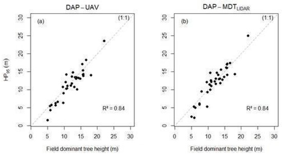
Figure 9.
Dispersion plots between the HP95 metric (95th percentile) obtained by (a) DAP and (b) DAP-DTMLiDAR compared with the dominant heights of the TFI plots.
The analysis of the graphs and statistics indicates that both DAP and DAP-DTMLiDAR have a tendency to underestimate dominant height values. There were no major differences between DAP and DAP-DTMLiDAR statistics, and the two methods presented similar accuracy. The tendency to underestimate height values occurred throughout the evaluation and not only in the places where the terrain control points were obtained [51], indicating the overestimation of DTM altitudes (see Section 3.2.1).
3.3. Selected Models
Multiple linear regression models were adjusted to estimate the values of mean h, dbh, and ba of individuals belonging to the 40 plots of traditional forest inventory. Several authors have evaluated the contribution of spectral data associated with photogrammetric point clouds in predicting forest attributes from a per-area approach and concluded that the benefit was negligible [54].
In a wide-ranging review conducted by Goodbody et al. [10], it was found that studies have shown that data from DAP point clouds can generate accurate forest inventories. The results obtained in this study further support that DAP is a reliable estimation method for average h, mean dbh, and ba in a per-area approach.
3.3.1. Average Total Height
Table 8 presents the models, which presented better performance in estimating the mean total h from DAP-UAV, LiDAR, and DAP-DTMLiDAR clouds. In general, all coefficients associated with the variables were significant, indicating that the predictor variables selected were related to the response variable. For all data sources, four metrics were selected as predictor variables.
Table 8.
Models selected to estimate average height from DAP-UAV, DAP-DTMLiDAR, and LiDAR.
Table 9 includes the statistics of the models selected to estimate h. The performances of the three data sources were satisfactory and similar, with DAP-DTMLiDAR presenting slightly higher errors (RMSE of 12.97%, 0.95 m); this indicates that, for this parameter, the use of hybrid data did not satisfactorily improve the estimates in the DAP point cloud. Gyawali et al. [55] also did not find significant differences between the estimation of height by DAP or LiDAR, corroborating the findings of the present study, which showed that DAP-UAV missed only 2.53% more than LiDAR (RMSE of 11.11%, 0.81 m, and RMSE of 8.58%, 0.63 m, respectively). Therefore, DAP data can be used to estimate mean height per RLM in a per-area approach, presenting results with quality comparable to LiDAR data.
Table 9.
Statistics from the fitting and validation of the best models for estimating average height (DAP-UAV, DAP-DTMLiDAR, and LiDAR).
The statistics presented in Table 9 corroborate the histograms of RMSE frequency observed in the validations of the models (Figure 10), presenting mean values similar to the RMSE values found in the fitting. The three methods presented normal distribution.
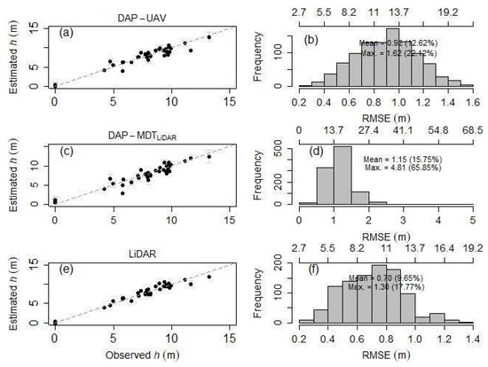
Figure 10.
Scatter plots between the estimated and observed mean h values for (a), (c), and (e) and the frequency histograms of RMSE in the validation of models (b), (d), and (f) for DAP, DAP-DTMLiDAR, and LiDAR.
In a review conducted by Goodbody et al. [56], the use of DAP point clouds normalized with LiDAR DTMs was recommended for updating enhanced inventories. In the present study, the performances presented by DAP-DTMLiDAR and DAP-UAV were similar, but there was a downgrade in relation to the results of DAP-UAV data alone. Thus, it is possible to adjust statistical models using DAP-UAV data reliably without the use of DTM’s LiDAR, depending on factors such as characteristics of the evaluated vegetation and quality of the photogrammetric survey.
3.3.2. Average dbh
The models that presented the best performance for dbh estimation are presented in Table 10 along with their respective variables. In general, all coefficients associated with the variables were significant, indicating that the predictor variables selected are related to the response variable. Four metrics were selected in all data sources as predictor variables for the best fit.
Table 10.
Best models to estimate average dbh from DAP-UAV, DAP-DTMLiDAR, and LiDAR.
Table 1 shows the statistics of the models selected to estimate the dbh. The three methods presented satisfactory performance in estimating diameter. As for h, DAP-DTMLiDAR yielded the worst performance, with RMSE of 18.14% and R² of 82.16%. Studies conducted by Shimizu et al. [57] found different results, indicating that the integration of photogrammetry data with LiDAR is beneficial for the estimation of forest attributes. DAP-UAV and LiDAR showed very similar results, with DAP-UAV presenting an RMSE of 12.23% and R² of 91.89% and LiDAR yielding an RMSE of 11.47% and R² of 92.87%
The statistics presented in Table 11 corroborate the histograms of RMSE frequency observed in the model validations (Figure 11) and present mean values similar to the adjusted RMSE values. The three methods presented normal distribution. These results corroborate those found by Moe et al. [58], which indicate that DAP-UAV can predict dbh values with accuracy comparable to the estimate performed with LiDAR data.
Table 11.
Fitting and validation statistics of the best models for estimating mean dbh from DAP-UAV, DAP-DTMLiDAR, and LiDAR.

Figure 11.
Dispersion plots between the estimated and observed average dbh values of (a,c,e), and the frequency histograms of RMSE in the validation of models (b,d,f), for DAP-UAV, DAP-DTMLiDAR, and LiDAR.
In general, fitting of RLM models for the estimation of average dbh from DAP, DAP-DTMLiDAR, and LiDAR point cloud data yielded reasonable results. The results found for DAP-DTMLiDAR data were lower than the other two methods. Studies conducted by Shimizu et al. [57] produced different results, indicating that the integration of photogrammetry data with LiDAR is beneficial for the estimation of forest attributes. DAP and LiDAR presented very similar fitting results, with DAP obtaining a slightly lower RMSE. These facts corroborate the results found by [55], which indicate that DAP can predict dbh values with accuracy comparable to the prediction performed with LiDAR data.
3.3.3. Basal Area (ba)
The models that presented the best adjusted performance for the estimation of ba from the DAP, DAP-DTMLiDAR, and LiDAR point clouds are presented in Table 12, along with their respective estimated parameters and variables. In general, all coefficients associated with the variables were significant, indicating that the predictor variables selected are related to the response variable. For fitting of the models for the three data sources, only three metrics were required as predictor variables.
Table 12.
Best models to estimate basal area from DAP-UAV, DAP-DTMLiDAR, and LiDAR.
Table 1 presents the statistics of the models selected to estimate ba. The three methods produced similar performances. Unlike h and dbh, the DAP estimation model presented the best results of RMSE and R² (%) in relation to the other two methods.
The statistics presented in Table 13 corroborate the histograms of RMSE frequency observed in the model validations (Figure 12) and present mean values similar to the RMSE values found in the fitting. The three methods presented normal distribution.
Table 13.
Fitting and validation statistics of the best models for estimating basal area from DAP-UAV, DAP-DTMLiDAR, and LiDAR.
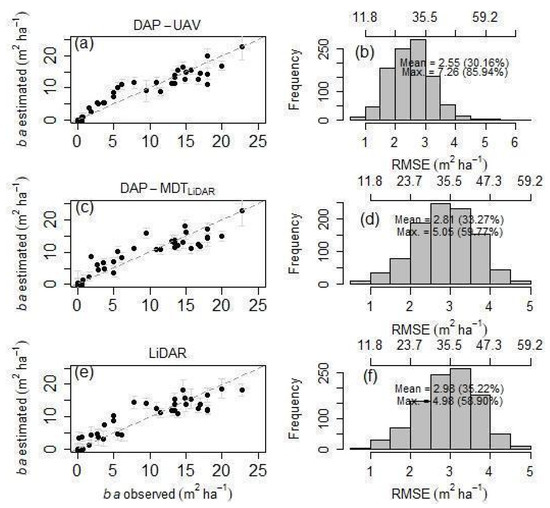
Figure 12.
Scatter plots between the estimated and observed ba values of (a,c,e), and the RMSE frequency histograms in the validation of models (b,d,f), for DAP-UAV, DAP-DTMLiDAR, and LiDAR.
The three methods proved to be reliable for estimating ba from statistical models obtained by multiple linear regression, corroborating what has been found in the literature. The integration of DAP data with LiDAR [59,60] was shown to be lower in relation to the use of DAP data exclusively for the estimation of this variable, in contrast to the findings observed by Ullah et al. [61], which found close results for LiDAR data and DAP data integrated with LiDAR DTM. In general, past studies have demonstrated better performances for LiDAR data. However, estimation using DAP data was higher than the use of LiDAR data in the present study [59,60,62].
3.4. Spatialization Maps of DAP-UAV Models
Figure 13 and Figure 14 display the maps resulting from the estimation of succession stages according to the parameters established by CONAMA Resolution 29/94 [27] after executing the procedures presented in Figure 4. Some areas met the criteria of both the initial and the middle stages, while others were simultaneously in the middle and advanced stages. These areas in transition were considered. In addition to the spatialization of stage estimation, Figure 13 and Figure 14 also present the plots and their respective stages according to CONAMA 29/94 [27]. For the plots where invasive species infestations were identified during the TFI, the acronyms for identification of the stages were added to the letter “E”.
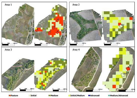
Figure 13.
Spatialization of the succession stage estimation for areas 1 to 4 based on DAP-UAV point clouds.
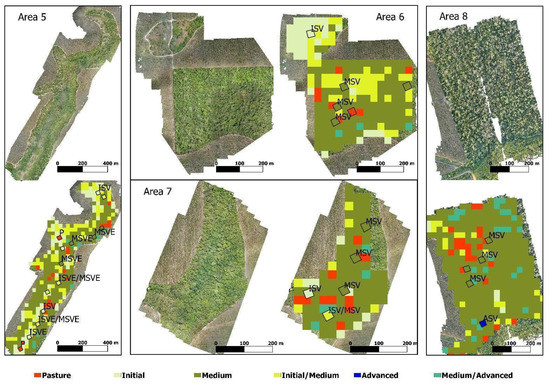
Figure 14.
Spatialization of succession stage estimation for areas 5 to 8 based on DAP-UAV point clouds.
3.5. Cost-Benefit Analysis
Table 14 presents the total costs of the classification of succession stages in the Atlantic Forest using DAP-UAV, LiDAR PLS, and TFI and their respective cost components. The tables with detailed values of the items and subcomponents of each methodology are presented in “Appendix A Table A1, Table A2, and Table A3”. LiDAR PLS presented the highest total cost at R$ 466,309.12, followed by TFI (R$ 136,009.94) and, finally, DAP-UAV (R$ 103,659.42).
Table 14.
Costs to obtain data by DAP-UAV, LiDAR PLS, and TFI.
Table 15 separates the costs of equipment acquisition and data acquisition and processing for the three methodologies. The high cost of LiDAR PLS is significantly influenced by equipment acquisition, which costs R$ 407,092.15. For DAP-UAV, equipment costs R$ 86,895.23, while for TFI it costs only R$ 41,443.94. Regarding the cost of data acquisition and processing per hectare, the sampling capacity and speed presented by DAP-UAV resulted in a considerably lower cost of R$ 83.40/ha versus the other methods (LiDAR PLS = R$ 16,449.16/ha, TFI = R$ 26,268.33/ha).
Table 15.
Equipment cost and cost per hectare for data acquisition using DAP-UAV, LiDAR PLS, and TFI.
Despite having lower equipment acquisition costs, TFI data acquisition operations are slow and have limited sampling capacity. The limitations inherent to TFI operations have increased their cost per hectare, as described by Navarro et al. [63] and Nogueira et al. [13], in addition to exposing operators to greater risks for longer periods of time. Currently, the cost of acquiring equipment for operations with LiDAR PLS is still very high, with the acquisition of the LiDAR system itself representing the main expense. The acquisition of forest inventory data by the LiDAR PLS method can be faster than in TFI, but it has great limitations in terms of size of the sampled area compared to DAP-UAV. [64,65,66] highlighted that PLS surveys for 3D modeling purposes have higher costs and require more field work, while DAP surveys for the same purposes are reliable and low-cost.
DAP has an intermediate cost of acquiring equipment when compared to the other two methods. As demonstrated, the cost of equipment for DAP operations can be approximately twice as high as TFI and approximately five times lower than PLS. However, DAP’s capacity regarding area to be sampled is significantly higher than that of PLS and TFI. While the samples for TFI and PLS were limited to the size of the plots, totaling 3.6 ha of sample for each method, the DAP can cover an area of 201 ha. Thus, DAP is suitable for forest use due to low operational costs and high coating intensity [67,68]. Naturally, the adoption of a methodology of LiDAR data collection with an aerial platform (ALS) would result in a sampling capacity similar to DAP. However, acquiring UAVs capable of operating with a LiDAR system would further increase equipment costs. This fact was confirmed by Kangas et al. [16] when they evaluated the cost of acquiring ALS and DAP data for forest decision-making and concluded that the higher accuracy of ALS does not significantly affect the results; therefore, ALS and DAP were equally recommended for forest management planning.
4. Conclusions
The collection of field data using the TFI method yielded suitable vegetation parameters for the correct identification of ecological succession stages in areas with secondary vegetation in the Atlantic Forest biome. In addition, the field data collected represented the structure of the study area, with data ranging from clean pastures to vegetation in advanced succession, thus offering a suitable source for adjusted statistical models.
DAP tends to overestimate the altitude of terrain, especially in an area of dense vegetation, thereby causing a tendency to underestimate the height of the point cloud. As such, it is not recommended to estimate heights via direct comparison with metrics of the DAP-UAV point cloud. However, high correlation with field data allowed adequate fitting of statistical models for the estimation of mean h, dbh at 1.30 m of soil, and ba, yielding results similar to those found using DAP data integrated with LiDAR data or using LiDAR data exclusively. The models obtained with DAP-UAV data permitted the creation of spatialization maps with h, dbh, and ba estimates in addition to spatialization of the stages of ecological succession.
DAP proved to be a technically effective and economically accessible method for estimating the forest attributes necessary for the classification of successional stages in the Atlantic Forest, demonstrating greater cost-effectiveness than LiDAR or TFI.
Author Contributions
R.P.C., G.F.d.S. and A.Q.d.A. conceived, designed, and performed the experiment; analyzed the data; and wrote the paper (original draft preparation, review and editing). A.R.D.M. conceived and designed the experiment; and wrote the paper (review); S.B.-B. wrote the paper (original draft preparation); H.M.D. and F.G.G. conceived, designed, and assisted with data collection. N.M.M.R., C.C.A.V. and K.O. assisted with data collection and contributed to parts of the analysis and writing of the paper (review and editing); T.S.S. conceived and designed the experiment. All authors have read and agreed to the published version of the manuscript.
Funding
This research was funded Espírito Santo Research and Innovation Support Foundation (FAPES), through the project “proposition of a protocol for identifying successional stages using remote sensing tools” process 2020-4KK4L and by Suzano S.A. and “The APC was funded by FAPES”.
Acknowledgments
The authors would like to thank CNPq for the research grant from the author André Q. Almeida of the project “Models for estimating biomass and other dendrometric characteristics of a secondary forest” process 310299/2019-5 and “TREEcarbon: Remote forest carbon monitoring system for the Atlantic Forest and Caatinga Biomes” process 300234/2022-8. We also thank Suzano S.A for making the study areas available and for all the support offered for the execution of this research. We would like to thank the Espírito Santo Research and Innovation Support Foundation (FAPES) (process 2020-4KK4L), and Espírito Santo Institute of Agricultural and Forestry Defense (IDAF), on behalf of Emaunel Effgen, for all the support offered for the execution of this research.
Conflicts of Interest
The authors declare no conflict of interest.
Appendix A
Table A1.
Traditional forest inventory cost components.
Table A1.
Traditional forest inventory cost components.
| Component | Sub-Component | Item | Quantity | Unit | Value | Total |
|---|---|---|---|---|---|---|
| Equipment | Equipment | Stakes | 1 | Ensemble | R$ 490.00 | R$ 490.00 |
| Equipment | Equipment | Telescopic ruler 15 m | 1 | Unit | R$ 500.00 | R$ 500.00 |
| Equipment | Equipment | Clinometer | 1 | Unit | R$ 1,899.00 | R$ 1,899.00 |
| Equipment | Equipment | Trena + nylon + measuring tape | 1 | Kit | R$ 186.55 | R$ 186.55 |
| Equipment | Equipment | Ppe | 3 | Kit | R$ 300.00 | R$ 900.00 |
| Equipment | Equipment | Computer Dell precision 3930 Rack + Monitor Dell 34" WQHD | 1 | Unit | R$ 35,722.23 | R$ 35,722.23 |
| Equipment | Software | Native Forest | 1 | License | R$ 1417.00 | R$ 1417.00 |
| Equipment | Software | Office Suite | 1 | License | R$ 329.16 | R$ 329.16 |
| Data acquisition | Data acquisition | Access to the parcel | 13 | Hour/man | R$ 459.00 | R$ 5967.00 |
| Data acquisition | Data acquisition | Plot demarcation | 59 | Hour/man | R$ 459.00 | R$ 27,081.00 |
| Data acquisition | Data acquisition | Data collection | 106 | Hour/man | R$ 459.00 | R$ 48,654.00 |
| Data acquisition | Data acquisition | Car Rental | 24 | Daily | R$ 224.00 | R$ 5376.00 |
| Data acquisition | Data acquisition | Host | 24 | Daily | R$ 210.00 | R$ 5040.00 |
| Data processing and analysis | Data processing and analysis | Data tabbing | 8 | Hour/man | R$ 153.00 | R$ 1224.00 |
| Data processing and analysis | Data processing and analysis | Data processing and analysis | 8 | Hour/man | R$ 153.00 | R$ 1224.00 |
| Total | 3.6 ha | R$ 136,009.94 | ||||
| Cost per hectare | Equipment | R$ 41,443.94 | ||||
| acquisition and analysis of data per hectare | 1 ha | R$ 26,268.33 |
Table A2.
Inventory cost components with terrestrial LiDAR.
Table A2.
Inventory cost components with terrestrial LiDAR.
| Component | Sub-Component | Item | Quantity | Unit | Value | Total |
|---|---|---|---|---|---|---|
| Equipment | Equipment | Horizom Zeb | 1 | Unit | R$ 367,700.00 | R$ 367,700.00 |
| Equipment | Equipment | Rent RTK | 160 | R$/dot | R$ 16.85 | R$ 2696.00 |
| Equipment | Equipment | Computer Dell precision 3930 Rack + Monitor Dell 34" WQHD | 1 | Unit | R$ 35,722.23 | R$ 35,722.23 |
| Equipment | Equipment | Machete | 3 | Unit | R$ 24.64 | R$ 73.92 |
| Equipment | Equipment | Ppe | 3 | Kit | R$ 300.00 | R$ 900.00 |
| Equipment | Software | Geoslam | 1 | License | R$ - | |
| Data acquisition | Data acquisition | Access to the parcel | 13 | Hour/man | R$ 459.00 | R$ 5967.00 |
| Data acquisition | Data acquisition | Data collection | 10 | Hour/man | R$ 459.00 | R$ 4590.00 |
| Data acquisition | Data acquisition | Collection of GCPs with RTK | 86,4 | Hour/man | R$ 459.00 | R$ 39,657.60 |
| Data acquisition | Data acquisition | Car Rental | 15 | Daily | R$ 224.00 | R$ 3360.00 |
| Data acquisition | Data acquisition | Hosting | 15 | Daily | R$ 210.00 | R$ 3150.00 |
| Data processing and analysis | Data processing and analysis | Point Clouds Processing | 6,6 | Hour/man | R$ 153.00 | R$ 1009.80 |
| Data processing and analysis | Data processing and analysis | Georeferencing of point clouds | 3,3 | Hour/man | R$ 153.00 | R$ 504.90 |
| Data processing and analysis | Data processing and analysis | Normalization of point clouds | 3,3 | Hour/man | R$ 153.00 | R$ 504.90 |
| Data processing and analysis | Data processing and analysis | Extraction of metrics | 1,76 | Hour/man | R$ 153.00 | R$ 269.28 |
| Data processing and analysis | Data processing and analysis | Application of models | 1,33 | Hour/man | R$ 153.00 | R$ 203.49 |
| Total | 3.6 ha | R$ 466,309.12 | ||||
| Cost per hectare | Equipment | R$ 407,092.15 | ||||
| acquisition and analysis of data per hectare | 1 ha | R$ 16,449.16 |
Table A3.
Inventory cost components with DAP.
Table A3.
Inventory cost components with DAP.
| Component | Sub-Component | Item | Quantity | Unit | Value | Total |
|---|---|---|---|---|---|---|
| Equipment | Equipment | DJI Mavic 2 pro + kit fly more + SD card | 1 | Unit | R$ 21,999.00 | R$ 21,999.00 |
| Equipment | Equipment | Rent RTK | 40 | R$/dot | R$ 16.85 | R$ 674.00 |
| Equipment | Equipment | Computer Dell precision 3930 Rack + Monitor Dell 34" WQHD | 1 | Unit | R$ 35,722.23 | R$ 35,722.23 |
| Equipment | Software | Agisoft | 1 | License | R$ 28,500.00 | R$ 28,500.00 |
| Data acquisition | Data acquisition | Flight planning | 1 | Hour/man | R$ 153.00 | R$ 153.00 |
| Data acquisition | Data acquisition | Collection of GCPs with RTK | 21,62 | Hour/man | R$ 459.00 | R$ 9923.58 |
| Data acquisition | Data acquisition | Flight | 1,45 | Hour/man | R$ 459.00 | R$ 665.55 |
| Data acquisition | Data acquisition | Car Rental | 5 | Daily | R$ 224.00 | R$ 1120.00 |
| Data acquisition | Data acquisition | Hosting | 5 | Daily | R$ 210.00 | R$ 1050.00 |
| Data processing and analysis | Data processing and analysis | Photo alignment | 2 | Hour/man | R$ 153.00 | R$ 306.00 |
| Data processing and analysis | Data processing and analysis | GPCs pointing | 2 | Hour/man | R$ 153.00 | R$ 306.00 |
| Data processing and analysis | Data processing and analysis | Point Cloud Cleanup | 1,33 | Hour/man | R$ 153.00 | R$ 203.49 |
| Data processing and analysis | Data processing and analysis | Dense cloud construction | 8,7 | Hour/man | R$ 154.00 | R$ 1339.80 |
| Data processing and analysis | Data processing and analysis | Normalization of point clouds | 8 | Hour/man | R$ 153,00 | R$ 1224.00 |
| Data processing and analysis | Data processing and analysis | Extraction of metrics | 1,76 | Hour/man | R$ 153.00 | R$ 269.28 |
| Data processing and analysis | Data processing and analysis | Application of models | 1,33 | Hour/man | R$ 153.00 | R$ 203.49 |
| Total | 201 ha | R$ 103,659.42 | ||||
| Cost per hectare | Equipment | R$ 86,895.23 | ||||
| acquisition and analysis of data per hectare | 1 ha | R$ 83.40 |
References
- ONU. Relatório Anual Das Nações Unidas No Brasil 2021–Portal ODS. Available online: https://portalods.com.br/publicacoes/relatorio-anual-das-nacoes-unidas-no-brasil-2021/ (accessed on 4 August 2022).
- Mma, M.d.M.A. ENREDD+ National REDD+ Strategy; Ministry of the Environment: Brasília, Brasil, 2016. [Google Scholar]
- Andrade, D.T.; Romeiro, A.R. Degradação Ambiental e Teoria Econômica. Rev. Econ. A 2011, 12, 3–26. [Google Scholar]
- Cunha, N.R.d.S.; Cunha, S.; Eustáquio De Lima, J.; Fernandes, M.; Gomes, M.; Braga, M.J. A Intensidade Da Exploração Agropecuária Como Indicador Da Degradação Ambiental Na Região Dos Cerrados, Brasil. Rev. De Econ. E Sociol. Rural. 2008, 46, 291–323. [Google Scholar] [CrossRef]
- Muñoz-Rojas, M.; Pereira, P.; Brevik, E.C.; Cerdà, A.; Jordán, A. Soil Mapping and Processes Models for Sustainable Land Management Applied to Modern Challenges. In Soil Mapping and Process Modeling for Sustainable Land Use Management; Elsevier: Amsterdam, The Netherlands, 2017; pp. 151–190. [Google Scholar]
- Dhakal, C.; Khadka, S.; Park, C.; Escalante, C.L. Climate Change Adaptation and Its Impact on Household Farm Income and Revenue Risk Exposure. Resour. Environ. Sustain. 2022, 10, 1–51. [Google Scholar] [CrossRef]
- DeVries, B.; Verbesselt, J.; Kooistra, L.; Herold, M. Robust Monitoring of Small-Scale Forest Disturbances in a Tropical Montane Forest Using Landsat Time Series. Remote Sens. Environ. 2015, 161, 107–121. [Google Scholar] [CrossRef]
- Campo, A.D.d.; Segura-Orenga, G.; Bautista, I.; Ceacero, C.J.; González-Sanchis, M.; Molina, A.J.; Hermoso, J. Assessing Reforestation Failure at the Project Scale: The Margin for Technical Improvement under Harsh Conditions. A Case Study in a Mediterranean Dryland. Sci. Total Environ. 2021, 796, 148952. [Google Scholar] [CrossRef] [PubMed]
- Pellico Netto, S.; Brena, D.A. Inventário Florestal, 1st ed.; UFPR: Curitiba, Brazil, 1997. [Google Scholar]
- Goodbody, T.R.H.; Coops, N.C.; Marshall, P.L.; Tompalski, P.; Crawford, P. Unmanned Aerial Systems for Precision Forest Inventory Purposes: A Review and Case Study. For. Chron. 2017, 93, 71–81. [Google Scholar] [CrossRef]
- Tompalski, P.; Coops, N.C.; White, J.C.; Wulder, M.A. Enhancing Forest Growth and Yield Predictions with Airborne Laser Scanning Data: Increasing Spatial Detail and Optimizing Yield Curve Selection through Template Matching. Forests 2016, 7, 255. [Google Scholar] [CrossRef]
- Higuchi, N.P.; dos Santos, J.; Jardim, F.C.S. Tamanho de Parcela Amostral Para Inventários Florestais. Acta Amaz. 1982, 12, 91–103. [Google Scholar]
- Nogueira, M.M.; Lentini, M.W.; Pires, I.P.; Bittencourt, P.G.; Zweede, J.C. Procedimentos Simplificados em Segurança e Saúde do Trabalho no Manejo Florestal Manual Técnico, 1st ed.; Instituto Floresta Tropical-Fundação Floresta Tropical: Belém, Brazil, 2010. [Google Scholar]
- White, J.C.; Coops, N.C.; Wulder, M.A.; Vastaranta, M.; Hilker, T.; Tompalski, P. Remote Sensing Technologies for Enhancing Forest Inventories: A Review. Can. J. Remote Sens. 2016, 42, 619–641. [Google Scholar] [CrossRef]
- Morin, D.; Planells, M.; Baghdadi, N.; Bouvet, A.; Fayad, I.; le Toan, T.; Mermoz, S.; Villard, L. Improving Heterogeneous Forest Height Maps by Integrating GEDI-Based Forest Height Information in a Multi-Sensor Mapping Process. Remote Sens. 2022, 14, 2079. [Google Scholar] [CrossRef]
- Kangas, A.; Gobakken, T.; Puliti, S.; Hauglin, M.; Næsset, E. Value of Airborne Laser Scanning and Digital Aerial Photogrammetry Data in Forest Decision Making. Silva Fennica 2018, 52, 1–19. [Google Scholar] [CrossRef]
- Pommerening, A. Approaches to quantifying forest structures. Forestry 2002, 75, 305–324. [Google Scholar] [CrossRef]
- Lorenzoni-Paschoa, L.; Abreu, K.M.P.; Silva, G.F.; Dias, H.M.; Machado, L.A.; Silva, L.D. Estágio sucessional de uma floresta estacional semidecidual secundária com distintos históricos de uso do solo no sul do Espírito Santo. Rodriguésia 2019, 70, 1–18. [Google Scholar] [CrossRef]
- Bergen, K.M.; Dronova, I. Observing succession on aspen-dominated landscapes using a remote sensing-ecosystem approach. Landsc. Ecol. 2007, 22, 1395–1410. [Google Scholar] [CrossRef]
- Bispo, P.D.C.; Pardini, M.; Papathanassiou, K.P.; Kugler, F.; Balzter, H.; Rains, D.; dos Santos, J.R.; Rizaev, I.G.; Tansey, K.; dos Santos, M.N.; et al. Mapping forest successional stages in the Brazilian Amazon using forest heights derived from TanDEM-X SAR interferometry. Remote. Sens. Environ. 2019, 232, 111194. [Google Scholar] [CrossRef]
- Kolecka, N.; Kozak, J.; Kaim, D.; Dobosz, D.; Ginzler, C.; Psomas, A. Mapping secondary forest succession on abandoned agricultural land with LiDAR point clouds and terrestrial photography. Remote Sens. 2015, 7, 8300–8322. [Google Scholar] [CrossRef]
- Myers, N.; Mittermeier, R.A.; Mittermeier, C.G.; da Fonseca, G.A.B.; Kent, J. Biodiversity hotspots for conservation priorities. Nature 2000, 403, 853–858. [Google Scholar]
- Ribeiro, M.C.; Metzger, J.P.; Martensen, A.C.; Ponzoni, F.; Hirota, M.M. BrazilianAtlantic forest: How much is left and how is the remaining forest distributed? Implications for conservation. Biol. Conserv. 2009, 142, 1141–1153. [Google Scholar] [CrossRef]
- INCAPER. Programa de Assistência Técnica e Extensão Rural, Proater 2020–2023; INCAPER: São Mateus, Brasil, 2020; pp. 1–55. [Google Scholar]
- Alvares, C.A.; Stape, J.L.; Sentelhas, P.C.; de Moraes Gonçalves, J.L.; Sparovek, G. Köppen’s Climate Classification Map for Brazil. Meteorol. Z. 2013, 22, 711–728. [Google Scholar] [CrossRef]
- IBGE. BDIA–Banco de Dados de Informações Ambientais. Available online: https://bdiaweb.ibge.gov.br/#/consulta/pedologia (accessed on 6 August 2022).
- Brasil. Resolução Conama 29, de 7 de dezembro de 1994 Conselho Nacional de Meio Ambiente. Available online: http://conama.mma.gov.br (accessed on 5 August 2022).
- Suunto PM-5/360 PC Clinometer–Inclination Tool for Professionals. Available online: https://www.suunto.com/Products/Compasses/Suunto-PM-5/Suunto-PM-5360-PC/ (accessed on 27 October 2022).
- Soares, C.P.B.; Paula Neto, F.; Souza, A.L. Dendrometria e Inventário Florestal; Editora UFV: Viçosa, Brazil, 2011. [Google Scholar]
- Dandois, J.P.; Olano, M.; Ellis, E.C. Optimal Altitude, Overlap, and Weather Conditions for Computer Vision UAV Estimates of Forest Structure. Remote Sens. 2015, 7, 13895–13920. [Google Scholar] [CrossRef]
- Brasil. ICA 100-40: Aeronaves não Tripuladas e o Acesso Aéreo Brasileiro. Available online: https://publicacoes.decea.mil.br/publicacao/ica-100-40 (accessed on 4 January 2023).
- Hung, M.N.W.B.; Sampaio, T.V.M.; Schultz, G.B.; Siefert, C.A.C.; Lange, D.R.; Marangon, F.H.S.; Santos, I. Dos levantamento com veículo aéreo não tripulado para geração demodelo digital do terreno em bacia experimental com vegetação florestal esparsa. RA’E GA–O Espac. Geogr. Em Anal. 2017, 39, 43–56. [Google Scholar] [CrossRef]
- Western Digital Corporation Cartão MicroSDXCTM SanDisk Extreme® PRO UHS-I, Melhor Cartão Micro SD|Western Digital. Available online: https://www.westerndigital.com/pt-br/products/memory-cards/sandisk-extreme-pro-uhs-i-microsd#SDSQXCD-128G-GN6MA (accessed on 7 August 2022).
- Agisoft Agisoft Metashape: Agisoft Metashape. Available online: https://www.agisoft.com/ (accessed on 7 August 2022).
- GEOSLAM ZEB Horizon: The Ultimate Mobile Mapping Solution. Available online: https://geoslam.com/solutions/zeb-horizon/ (accessed on 7 August 2022).
- GEOSLAM GeoSLAM Hub: Transform 3D Data into Actionable Information. Available online: https://geoslam.com/hub/ (accessed on 7 August 2022).
- Roussel, J.-R.; Auty, D.; Coops, N.C.; Tompalski, P.; Goodbody, T.R.H.; Meador, A.S.; Bourdon, J.-F.; de Boissieu, F.; Achim, A. LidR: An R Package for Analysis of Airborne Laser Scanning (ALS) Data. Remote Sens. Environ. 2020, 251, 112061. [Google Scholar] [CrossRef]
- R Core Team R: The R Project for Statistical Computing. Available online: https://www.r-project.org/ (accessed on 7 August 2022).
- McGaughey, R. FUSION/LDV: Software for LIDAR Data Analysis and Visualization 2022. V3.42; USDA Forest Service: Washington, DC, USA, 2022; pp. 1–212. [Google Scholar]
- Almeida, A.; Gonçalves, F.; Silva, G.; Souza, R.; Treuhaft, R.; Santos, W.; Loureiro, D.; Fernandes, M. Estimating Structure and Biomass of a Secondary Atlantic Forest in Brazil Using Fourier Transforms of Vertical Profiles Derived from UAV Photogrammetry Point Clouds. Remote Sens. 2020, 12, 3560. [Google Scholar] [CrossRef]
- Lumley, T. Package “Leaps”: Regression Subset Selection. Available online: https://cran.r-project.org/web/packages/leaps/leaps.pdf (accessed on 4 February 2022).
- SEEA; AEFES; CREA-ES. Tabela de Serviços e Honorários Profissionais No Campo Da Engenharia Agronômica Para o Estado Do Espírito Santo; SEEA: Vitória, Brazil, 2012. [Google Scholar]
- Gil, A.L.; Núñez-Casillas, L.; Isenburg, M.; Benito, A.A.; Bello, J.J.R.; Arbelo, M. A Comparison between LiDAR and Photogrammetry Digital Terrain Models in a Forest Area on Tenerife Island. Can. J. Remote Sens. 2013, 39, 396–409. [Google Scholar] [CrossRef]
- Zahawi, R.A.; Dandois, J.P.; Holl, K.D.; Nadwodny, D.; Reid, J.L.; Ellis, E.C. Using Lightweight Unmanned Aerial Vehicles to Monitor Tropical Forest Recovery. Biol. Conserv. 2015, 186, 287–295. [Google Scholar] [CrossRef]
- Panagiotidis, D.; Abdollahnejad, A.; Surový, P.; Chiteculo, V. Determining Tree Height and Crown Diameter from High-Resolution UAV Imagery. Int. J. Remote Sens. 2017, 38, 2392–2410. [Google Scholar] [CrossRef]
- Mlambo, R.; Woodhouse, I.; Gerard, F.; Anderson, K. Structure from Motion (SfM) Photogrammetry with Drone Data: A Low Cost Method for Monitoring Greenhouse Gas Emissions from Forests in Developing Countries. Forests 2017, 8, 68. [Google Scholar] [CrossRef]
- Guerra-Hernández, J.; González-Ferreiro, E.; Monleón, V.; Faias, S.; Tomé, M.; Díaz-Varela, R. Use of Multi-Temporal UAV-Derived Imagery for Estimating Individual Tree Growth in Pinus Pinea Stands. Forests 2017, 8, 300. [Google Scholar] [CrossRef]
- Kachamba, D.; Ørka, H.; Gobakken, T.; Eid, T.; Mwase, W. Biomass Estimation Using 3D Data from Unmanned Aerial Vehicle Imagery in a Tropical Woodland. Remote Sens. 2016, 8, 968. [Google Scholar] [CrossRef]
- Alcudia-Aguilar, A.; Alcudia-Aguilar, A.; Martínez-Zurimendi, P.; van der Wal, H.; Castillo-Uzcanga, M.M.; Suárez-Sánchez, J. Allometric Estimation of the Biomass of Musa spp. in Homegardens of Tabasco, Mexico. Trop. Subtrop. Agroecosyst. 2019, 22, 143–152. [Google Scholar]
- Meng, R.; Wu, J.; Schwager, K.L.; Zhao, F.; Dennison, P.E.; Cook, B.D.; Brewster, K.; Green, T.M.; Serbin, S.P. Using High Spatial Resolution Satellite Imagery to Map Forest Burn Severity across Spatial Scales in a Pine Barrens Ecosystem. Remote Sens. Environ. 2017, 191, 95–109. [Google Scholar] [CrossRef]
- Ganz, S.; Käber, Y.; Adler, P. Measuring Tree Height with Remote Sensing—A Comparison of Photogrammetric and LiDAR Data with Different Field Measurements. Forests 2019, 10, 694. [Google Scholar] [CrossRef]
- Dandois, J.P.; Ellis, E.C. High Spatial Resolution Three-Dimensional Mapping of Vegetation Spectral Dynamics Using Computer Vision. Remote Sens. Environ. 2013, 136, 259–276. [Google Scholar] [CrossRef]
- Schneider, P.R.; Schneider, P.S.P. Introdução Ao Manejo Florestal, 2nd ed.; FACOS-UFSM: Santa Maria, Brazil, 2008; ISBN 978-85-98031-51-4. [Google Scholar]
- Tompalski, P.; White, J.C.; Coops, N.C.; Wulder, M.A. Quantifying the Contribution of Spectral Metrics Derived from Digital Aerial Photogrammetry to Area-Based Models of Forest Inventory Attributes. Remote Sens. Environ. 2019, 234, 111434. [Google Scholar] [CrossRef]
- Gyawali, A.; Aalto, M.; Peuhkurinen, J.; Villikka, M.; Ranta, T. Comparison of Individual Tree Height Estimated from LiDAR and Digital Aerial Photogrammetry in Young Forests. Sustainability 2022, 14, 3720. [Google Scholar] [CrossRef]
- Goodbody, T.R.H.; Coops, N.C.; White, J.C. Digital Aerial Photogrammetry for Updating Area-Based Forest Inventories: A Review of Opportunities, Challenges, and Future Directions. Current Forestry Reports. 2019, 5, 55–75. [Google Scholar] [CrossRef]
- Shimizu, K.; Nishizono, T.; Kitahara, F.; Fukumoto, K.; Saito, H. Integrating Terrestrial Laser Scanning and Unmanned Aerial Vehicle Photogrammetry to Estimate Individual Tree Attributes in Managed Coniferous Forests in Japan. Int. J. Appl. Earth Obs. Geoinf. 2022, 106, 102658. [Google Scholar] [CrossRef]
- Moe, K.T.; Owari, T.; Furuya, N.; Hiroshima, T.; Morimoto, J. Application of UAV Photogrammetry with LiDAR Data to Facilitate the Estimation of Tree Locations and DBH Values for High-Value Timber Species in Northern Japanese Mixed-Wood Forests. Remote Sens. 2020, 12, 2865. [Google Scholar] [CrossRef]
- Kukkonen, M.; Maltamo, M.; Packalen, P. Image Matching as a Data Source for Forest Inventory–Comparison of Semi-Global Matching and Next-Generation Automatic Terrain Extraction Algorithms in a Typical Managed Boreal Forest Environment. Int. J. Appl. Earth Obs. Geoinf. 2017, 60, 11–21. [Google Scholar] [CrossRef]
- Iqbal, I.A.; Musk, R.A.; Osborn, J.; Stone, C.; Lucieer, A. A Comparison of Area-Based Forest Attributes Derived from Airborne Laser Scanner, Small-Format and Medium-Format Digital Aerial Photography. Int. J. Appl. Earth Obs. Geoinf. 2019, 76, 231–241. [Google Scholar] [CrossRef]
- Ullah, S.; Dees, M.; Datta, P.; Adler, P.; Schardt, M.; Koch, B. Potential of Modern Photogrammetry Versus Airborne Laser Scanning for Estimating Forest Variables in a Mountain Environment. Remote Sens. 2019, 11, 661. [Google Scholar] [CrossRef]
- Gobakken, T.; Bollandsås, O.M.; Næsset, E. Comparing Biophysical Forest Characteristics Estimated from Photogrammetric Matching of Aerial Images and Airborne Laser Scanning Data. Scand. J. For. Res. 2015, 30, 73–86. [Google Scholar] [CrossRef]
- Navarro, A.; Young, M.; Allan, B.; Carnell, P.; Macreadie, P.; Ierodiaconou, D. The Application of Unmanned Aerial Vehicles (UAVs) to Estimate above-Ground Biomass of Mangrove Ecosystems. Remote Sens. Environ. 2020, 242, 111747. [Google Scholar] [CrossRef]
- Pereira, I.S. Desempenho de Dispositivos Eletrônicos para Análise Estrutural da floresta de terra firme na Amazônia Central; Instituto nacional de pesquisas da Amazônia–INPA: Manaus, Brazil, 2018. [Google Scholar]
- Berbert, M.L.D.G. Potencial do LiDAR Terrestre Como Ferramenta para o Manejo de Florestas Naturais; UFRRJ: Seropédica, Brazil, 2016. [Google Scholar]
- Araújo, J.P.d.C.; Niemann, R.S.; Dourado, F.; Fernandes, M.C.; Fernandes, N.F. Revisões de Literatura de Geomorfologia Brasileira; UnB: Brasília, Brasil, 2022. [Google Scholar]
- Pires, P.F. Geociências, Sociedade e Sustentabilidade, 1st ed.; Conhecimento Livre: Piracanjuba, Brasil, 2020. [Google Scholar]
- Tang, L.; Shao, G. Drone Remote Sensing for Forestry Research and Practices. J. For. Res. 2015, 26, 791–797. [Google Scholar] [CrossRef]


Disclaimer/Publisher’s Note: The statements, opinions and data contained in all publications are solely those of the individual author(s) and contributor(s) and not of MDPI and/or the editor(s). MDPI and/or the editor(s) disclaim responsibility for any injury to people or property resulting from any ideas, methods, instructions or products referred to in the content. |
© 2023 by the authors. Licensee MDPI, Basel, Switzerland. This article is an open access article distributed under the terms and conditions of the Creative Commons Attribution (CC BY) license (https://creativecommons.org/licenses/by/4.0/).