Abstract
Total phosphorus (TP) is the main limiting factor of eutrophication for most inland waters globally. However, the combination of the limited temporal-spatial ranges of traditional manual sampling, poor spectral resolutions, and weather-vulnerable satellite observations, have yielded great data gaps in TP dynamics in short-lived, extreme episodic, or unpredictable pollution. Hence, a novel ground-based hyperspectral proximal sensing system (GHPSs) with a maximum observation frequency of 20 s and a spectral resolution of 1 nm between 400 and 900 nm was developed for automatic, real-time and continuous observation of TP. Focusing on the GHRSs, a TP machine learning model was developed and validated with ideal accuracy (R2 = 0.97, RMSE = 0.017 mg·L−1, MAPE = 12.8%) using 377 pairs of in situ TP measurements collected from Fuchunjiang Reservoir (FR), Liangxi River (LR), and Lake Taihu (LT). Second-scale TP results showed a low-value stable period followed by a sharp change period in LT during 29–31 October and 1–3 November, respectively. The exponential increase (R2 = 0.65, p < 0.05) on 1 November and the two complete variations with peak values of 0.32 mg·L−1 and 0.42 mg·L−1 were recorded in LT on 2 and 3 November, respectively. Simultaneously, a significant decrease (R2 = 0.57, p < 0.05) over the observation days was observed in LR and no obvious change was observed in FR. High consistency between the GHPSs spectrum data standardized at 574 nm and the measured reflectance in different weather demonstrated the accuracy of the GHPSs spectrum data (R2 > 0.99, slop = 0.98). Short and rapid TP changes were observed within one day in LT and LR based on GHPSs minute scale monitoring, which highlighted the importance of high frequency observations of TP. Several advantages of real-time, high accuracy and wide applicability to complex weather were highlighted for the GHPSs for TP monitoring compared to traditional equipment. Therefore, there are potential applications of the GHPSs in the integrated space-air-ground TP monitoring, as well as emergency monitoring and early-warning systems in the future, and it can raise our awareness of the dynamics and driving mechanisms of water quality for inland waters.
1. Introduction
Phosphorus, an indispensable nutrient, is known as the main restriction factor of eutrophication in freshwater ecosystems [1,2,3,4,5]. However, with anthropogenic activities and economic development, increasing amounts of phosphorus have been discharged into water from industrial and domestic sewage, as well as agricultural activities, resulting in water quality decline and eutrophication of inland waters [6,7,8,9,10]. Enrichment of phosphorus and eutrophication has further triggered abnormal harmful algae proliferation and odor compounds that have imposed threats to drinking water [11,12,13]. Consequently, to strengthen sustainable water environment management, high-frequency continuous observation and timely quantitation of total phosphorus (TP) are important prerequisites that are urgently required for effectively monitoring and controlling eutrophication [14,15]. However, spatiotemporal heterogeneity and environmental sensitivity of water quality in lakes and rivers bring great challenges to obtain effective and high-frequency TP data in short-lived, extreme episodic, or unpredictable pollution [14,16]. Hence, it is necessary to obtain high-frequency information on the time, extent, acceptable level, and potential influencing factors of TP variations, which is essential for forecasting the trends and developing appropriate mitigation strategies.
However, the main existing monitoring methods and measurement equipment for TP have lagged behind the needs of water environment management and decision-making departments in terms of data collection frequency, timeliness and representativeness, especially for sudden TP pollution events. Low frequency, time-consuming and labor-intensive traditional manual sampling makes it difficult to timely capture rapid dynamics of meteorological- and human-induced TP in lakes and rivers. Especially, during emergencies and extreme weather, the available manual sampling is often lacking [15,17,18]. A commercial automatic sensor with high-temperature/pressure digestion and phosphor molybdenum blue has been involved in rapid and continuous TP monitoring [19,20]. Unfortunately, long digestion times (more than 15 min), high-temperature or pressure conditions and digestion reagents resulted in low monitoring frequency, adhesive pollution, and secondary environmental pollution [19,20,21], all of which limited its wide application. Furthermore, in the past two decades, satellite remote sensing has widely been used to estimate water quality parameters due to its advantages of large area coverage, periodicity, and cost-efficiency. Although TP has no clear spectral signal characteristics, empirical and machine learning models combining its complex coupling relationship with optically active substances have made it feasible to do remote sensing of TP estimation [22,23]. Nevertheless, the limited spatial-temporal resolution and sensitivity to complex weather conditions (overcast, cloudy and rainy) of satellites has resulted in insufficient available data to obtain the dynamics of TP, especially those which change rapidly over a few hours due to any of a large number of pollutants from a catchment entering the receiving lakes and reservoirs [16,24,25,26]. Moreover, the mutually restricted spectral resolution and spatial resolution of satellites has also limited its application in small and micro water bodies with weak buffer capacity [27,28]. The flexible and mobile unmanned aerial vehicle (UAVs) hyperspectral remote sensing has partially made up for the above defects, but limited hover time and complex weather hinders continuous monitoring [29].
Therefore, developing real-time, high-frequency, continuous and reliable TP monitoring equipment that operates in complex weather conditions is the primary challenge to be solved. In such conditions, an automatic and real-time ground-based hyperspectral proximal sensing system (GHPSs) with high temporal and spectral resolution was developed for water quality monitoring under different weather conditions. In general, the design concept of the GHPSs is that based on 4G (or 5G) online transmission. The terminal computer (or mobile phone) displays the TP dataset, which was calculated from the pre-developed TP estimation model and real-time spectrum gathered from a fixed high-frequency hyperspectral imager that can operate during complex weather conditions. Among the requirements, obtaining accurate hyperspectral irradiance ratio data is the foundation, and developing an accurate and robust TP estimation model is integral. Real-time and high-frequency TP data provides decision support for scientific and effective water environment management and emergency warning.
In this paper, we first propose a high-frequency, real-time automated equipment, namely the GHPSs, and elucidate its feasibility, advantages, and potential applications for tracking TP dynamics. Specifically, our aims were to (1) develop and validate a TP model using the GHPSs and in situ data, (2) reconstruct the TP minute-scale time-series datasets and finely characterize the short-term dynamic process of TP, and (3) discuss in detail the reliability and stability of the GHPSs spectrum for TP estimation under different weather conditions, and to further expound the advantages and potential application of the GHPSs in tracking the variation of TP and as an emergency early warning system in the future.
2. Materials and Methods
2.1. Study Area
Considering the complexity and diversity of the water quality in different inland waters, the eutrophic Lake Taihu (LT), the mesotrophic Fuchunjiang Reservoir (FR), and the urban river Liangxi River (LR) were selected as the study areas of enriched water sample types (Figure 1a). Lake Taihu (30.93°–31.55°N, 119.88°–120.60°E), one of five largest freshwater lake in China, has suffered from severe eutrophication and a cyanobacteria bloom since the 1970s [30,31]. Strict governance policies were implemented after 2007, but TP has experienced a fluctuation of first decreasing and then increasing eutrophication, indicating that it has not been effectively alleviated [32]. Liangxi River (31.550°N, 120.243°E), located in Wuxi city, is one of the main outflow rivers of the northern LT, which outputs eutrophic water from the lake to Meiliang Bay to prevent further deterioration of water quality [33,34]. However, the high nutrient load in the water and the cyanobacteria bloom not only worsened the water quality of the network of urban rivers but also destroyed the townscape [35]. Fuchunjiang Reservoir (29.683°N, 119.643°E) is a river-style reservoir between Xin’anjiang Reservoir and Qiantang River [36]. However, the outbreaks of large-scale cyanobacteria blooms in 2004, 2016 and 2017 has attracted extensive attention from scholars, and urgently required control of the nutrient input to ensure a safe water quality [37,38].
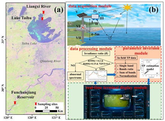
Figure 1.
Location of three monitoring sites (a); the framework of the GHPSs and workflow of real-time observation for TP (b) (I. high-definition video monitoring; II. lower spectrometer; III. ambient light sensor; IV. upper spectrometer; V. solar panel; VI. power and data storage; VII. bracket).
2.2. GHPSs Framework
Figure 1b shows the framework of the GHPSs and workflow for monitoring TP. In general, it is composed of four modules, namely a data acquisition module, a data processing module, a parameter inversion module, and a real-time terminal display module. First, real-time and high-frequency hyperspectral data of water bodies were automatically and stably collected by the data acquisition module installed in field lakes, reservoirs, and rivers according to the proposed acquisition frequency. These were then transferred to the data processing module to eliminate the abnormal spectrum caused by wood block, leaves and floating garbage, etc. After that, the remaining spectra were applied to the parameter inversion module with the built-in TP estimation model to obtain the time series dataset for high-frequency TP. Finally, it was transmitted through a 4G (or 5G) network and displayed in terminal modules such as computers or mobile phones. All data calculations and processes were completed by an embedded artificial intelligence chip. As one of the core modules, the basic principle of the parameter inversion module is to isolate the sensitive band containing the material components and their concentration for the water body from the spectrum and to then retrieve water quality parameters following the relationship between the sensitive band and the water component and concentration.
2.3. Field Data Collection and Measurement
The in situ dataset contained 172, 96, and 109 water samples, which were sampled at LT, LR and FR every 10 or 15 min during the three time periods 28 October to 3 November, 7 to 9 November, and 10 to 13 November 2020, respectively (Figure 1a). The mixed water column was collected by a 2.5 L acid-cleaned plastic water collector within the range of 0 m to 0.5 m below the water surface. All the water samples were preserved in the dark at 4 °C and immediately transported to the laboratory and, within 24 h, chlorophyll a (Chla), suspended particulate matter (SPM), total nitrogen (TN), and TP was measured in the Taihu Laboratory for Lake Ecosystem Research. After being filtered through Whatman GF/F fiberglass filters, samples for Chla extracted in 90% ethanol at 80 °C for 4 h were determined the difference in optical density between 665 nm and 750 nm measured by a Shimadzu UV-2550 PC UV–Vis spectrophotometer [27,39]. After pre-burning at 550 °C for 4 h and pre-weighed by an electronic balance, then the Whatman GF/F fiberglass filters containing SPM with a pore size of 0.7 were baked at 105 °C for 4 h and reweighed, and the finally the SPM was calculated. After the samples were decomposed by alkaline potassium persulfate obeying the “Standard Methods for the Examination of Water and Wastewater”, the TN and TP were measured by a Shimadzu UV-2550 PC UV-Vis spectrophotometer [24,40].
In addition, according to the above-water method, 8, 7 and 5 the remote-sensing reflectance (Rrs(λ), sr−1) were respectively collected during sunny, cloudy and overcast weather using an Analytical Spectral Devices spectroradiometer (ASD, Inc., Boulder, CO) with 1 nm interval between 350 and 2500 nm [41] on 4, 8 and 9 November 2021. According to the above-water method, Rrs(λ) was defined as the ratio of upwelling water-leaving radiance to downwelling irradiance [41]. There were three steps to measure it: (1) the downwelling radiance was an average value of the downwelling radiance collected from the reference panel twice, namely Lp; (2) then the total upwelling radiance above the water surface (Lt) was measured with a nadir view angle of 45° and an azimuth angle of 135°; (3) after that, the downwelling sky radiance (Lsky) was measured by the spectrometer rotated upwards to 90°. Notably, ten radiance spectra were collected every time to eliminate random error. Rrs(λ) was calculated by the following formula.
where Lt denotes the total upwelling radiance above the water surface (W·m−2·sr−1); rsky represents the skylight reflectance at the air-water surface, taken as 2.2% for calm weather, 2.5% for wind speed lower than 5 m/s, and 2.6% to 2.8% for wind speed of about 10 m/s [41]. Lsky is the downwelling sky radiance (W·m−2·sr−1); (W·m−2·sr−1) and ρρ are the downwelling radiance and the reflectance collected from the reference panel.
Rrs(λ) = (Lt − rsky × Lsky)/(Lp × π/ρρ)
2.4. GHPSs Dataset and Preprocessing
Relying on the instrument support system of the GHPSs, spectrum data under complex weather were continuously and stably collected by a high-resolution spectrometer placed at a height of approximately 4 m above the surface of water and 2–5 m away from the shore. The spectrometer had a field of view of 3° with a spectral resolution of 1 nm between 400 nm and 1000 nm at the highest frequency of 20 s. In this study, the monitoring temporal resolution for LT was set to 30 s, while those for LR and FR were set to 1 min, which met the different monitoring needs to reconstruct the second-minute TP dataset. The GHPSs datasets were acquired between 8:30 and 16:30 to avoid sensor deviation and low sunlight. Notably, the irradiance ratio (R(λ)) collected from the GHPSs was the ratio of upwelling and downwelling irradiance above the water surface measured synchronously by the upper and lower spectrometers, which was different from Rrs(λ). In addition, upwelling and downwelling irradiance above the water surface were corrected by the ambient light sensor combining a convolutional neural network algorithm to minimize the influence of the skylight and the solar altitude angles (Figure 1). The R(λ) was derived according to the following formula:
where Eu and Ed denote the upwelling and the downwelling irradiance at λ nm gathered from the GHPSs (W·m−2), respectively.
Two preprocessing programs were used to eliminate abnormal spectra. First, the R(λ) of 900–1000 nm was eliminated according to the low signal-to-noise ratio. The effective bands spanning 400–900 nm were selected to develop and validate the TP model. Second, to eliminate abnormal spectrum data caused by leaves, wood blocks and floating vegetation, the R(λ) at 550 nm and 880 nm were determined to be lower than 0.2 and 0.5, respectively, by analyzing the spectrum data from the three study areas. Moreover, given the spectral characteristics of cyanobacteria pigments with high absorption in the red band and high reflection in the near-infrared band, the Normalized Difference Vegetation Index (NDVI) was introduced to detect and eliminate the abnormal spectrum data of cyanobacteria blooms completely covering the water surface and obstructing water quality information. The spectrum data was removed when the NDVI was greater than 0.4 (corresponding to Chla > 200 μg·L−1) via the following equation:
where R(λ) represents the irradiance ratio at λ nm collected from GHPSs.
2.5. Matchups between the GHPS and Field Data
Ideally, the temporal and spatial satellite and field data should be synchronized when the natural variation of the water body was observed [42,43]. Therefore, to ensure minimum error caused by the temporal and spatial difference, we set a spatio-temporal criterion for matching between the GHPSs data and the field data to ≤30 s and ≤0.1 m (the time interval and the distance between the field dataset and the corresponding GHPSs dataset). Our criterion generated 377 pairs of effective matching data to develop and validate a TP estimation model. Subsequently, considering the robustness and applicability of the TP estimation model development and validation, we randomly selected two-thirds of the matching data for developing models and the rest served for validating the performance of the model.
2.6. Empirical Method and Machine Learning Method
Currently, there are two major methods for estimating TP, namely the empirical method and the machine learning method [14,44,45]. Generally, developing an empirical model required two steps: (1) selecting the most sensitive spectral index to the measured TP from a series of spectral indices, and (2) determining the relationship between the optimal spectral indexes and the measured TP with the highest R2 and lowest error according to linear and nonlinear fitting functions such as linear, logarithmic, exponential, and power formulations [46,47]. Considering the complex relationship between TP and optically active substances may not be expressed by linear or nonlinear, the machine learning method was introduced to directly estimate TP [44]. Extreme gradient boosting (XGBoost) is an extensible gradient boosting model, which continuously adds trees to segmentation features until the stop criteria are reached, and achieves the final prediction by summing the importance score in each tree [48]. Compared to the other gradient boosting models, the regularization process, algorithmic parallel, and distributed computing of the XGBoost technique, reduce overfitting and improve the learning rate and the robustness of noise prediction [48], which makes the model widely used in water quality estimation [49,50].
2.7. Classification of Lake and River
The water of lakes (including reservoirs) and rivers can be divided into six types according to TP pollution in Environmental Quality Standard for Surface Water (https://www.mee.gov.cn/ywgz/fgbz/bz/bzwb/shjbh/shjzlbz/200206/W020061027509896672057.pdf (accessed on 13 August 2022)). Specific classification thresholds are given in Table 1.

Table 1.
The classification thresholds of six water types according to TP.
2.8. Statistics Analysis and Accuracy Assessment
Statistical analyses, including maximum, minimum, mean and standard deviation (S.D.), were conducted using the Statistical Program for Social Sciences (SPSS 22.0). Moreover, the Pearson correlation coefficient (r), regressions analysis, and nonparametric tests were performed to analyze the relationship between the measured and estimated data. Statistical significance was defined as p ≤ 0.05. The coefficient of determination (R2), mean absolute percentage error (MAPE), root mean square error (RMSE) and relative error (RE) were calculated as the following formulas to evaluate the performance and accuracy of the TP model.
where n denotes the number of samples, Yi,m represents the measured value and Yi,e represents the estimated values.
3. Results
3.1. Water Quality Conditions
Table 2 gives the summary statistics for the measured water quality data of LT, LR, and FR. Overall, obvious differences in water quality were conducive to establishing a robust TP estimation model. The SPM of samples ranged from 6.92 mg·L−1 to 127.83 mg·L−1, with a mean value of 33.49 ± 18.96 mg·L−1 (mean ± standard deviation, the same below); TN varied from 0.93 mg·L−1 to 6.37 mg·L−1 (1.66 ± 0.73 mg·L−1); the range of TP was from 0.04 mg·L−1 to 0.62 mg·L−1 (0.11 ± 0.08 mg·L−1); Chla changed from 0.07 to 442.94 μg·L−1, with a mean value of 35.76 ± 57.65 μg·L−1. Specifically, significant differences in water quality among different study areas were found. The mean values of TP, SPM, and Chla in LT and LR were significantly higher than those in FR (p ≤ 0.05), indicating that the water of FR has the lowest nutrient load and phytoplankton biomass (Table 2).
Table 2.
Statistical analyses of in situ measurements were collected from three study areas.
In addition, significant positive correlations were found between TP and TN, and SPM and Chla, in LT and LR, while TP in FR was only significantly correlated with TN and SPM (p < 0.05) but not significant with Chla (p > 0.05). The results revealed that phytoplankton and SPM were important factors affecting TP in LT and LR, while TP in FR was mainly related to other factors other than phytoplankton.
3.2. Model Development and Validation
The dataset containing 252 field samples with a range of 0.04 mg·L−1 to 0.62 mg·L−1, and a mean value of 0.11 ± 0.08 mg·L−1 was used to develop the TP estimation model. The developed models were evaluated by the independent analysis of 125 pairs of matching datasets with a TP mean value of 0.11 ± 0.08 mg·L−1.
To obtain the optimal empirical model, five spectral indexes including single band, band ratio, sum or difference of two bands, and normalized different index, were used to fit in situ TP. Consequently, Table 3 shows that the R2 of four fitting functions between the five optimal spectral indices and the measured TP ranged from 0.53 to 0.85 based on the empirical method. Among these models, the linear and power function models (Formulas (7) and (8)) based on the ratio of 740 nm and 670 nm had the highest R2 value of 0.85 and RMSE values of 0.030 mg·L−1 and 0.032 mg·L−1, respectively, while the MAPE values were 15.0% and 14.5% (Figure 2a,c). The developed models were expressed by the following equations:
TP = 0.1965 × R(740)/R(670)) + 0.027 R2 = 0.85, p < 0.001
TP = 0.1872 × (R(740)/R(670))0.9048 R2 = 0.85, p < 0.001
Table 3.
The R2 of four fitting models for TP with optimal spectral indexes.
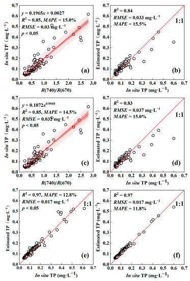
Figure 2.
Scatterplots of development (n = 252) and validation (n = 125) based on TP linear model (a,b), power exponential model (c,d) and the XGBoost model (e,f).
Moreover, machine learning model estimation was carried out. First, to reduce the calculation and accelerate the model convergence, we selected the bands with an interval of 10 nm between 400 and 900 nm and the five optimal spectral indices (Table 3) as the input characteristics. Then, the TP machine learning model based on the XGBoost method was obtained with the highest R2 of 0.97 as well as the lowest RMSE and MAPE of 0.017 mg·L−1 and 12.8% (Figure 2e).
To validate the accuracy and robustness of the TP estimation model, the R2, RMSE and MAPE of the three models were calculated based on the validation datasets (Table 4). The XGBoost model exhibited higher accuracy (R2 = 0.97, RMSE = 0.017 mg·L−1, MAPE = 11.8% and the RE of 84.0% samples lower than 20%) than the linear model (R2 = 0.84, RMSE = 0.033 mg·L−1, MAPE = 15.5% and the RE of 75.2% samples lower than 20%) and power function model (R2 = 0.83, RMSE = 0.037 mg·L−1, MAPE =15.0% and RE of the 74.4% samples lower than 20%) (Figure 2b,d,f). In addition, compared with the models based on the ratio of 740 nm and 670 nm, the retrieved TP values based on the XGBoost estimation model and the in situ TP were evenly distributed around the 1:1 line. The result implied that the developed XGBoost models performed well in estimating TP from GHPSs data. To further verify the superiority of our model, we introduced three published TP models for comparison (Table 4). Among the six models, our XGBoost TP model outperformed the YH-model proposed by Xiong et al. (R2 = 0.64, RMSE= 0.06 mg·L−1 and MAPE = 34.13%), the semi-analytical TP model proposed by Du et al. based on the absorption of 675 nm (R2 = 0.87, RMSE= 0.04 mg·L−1 and MAPE = 16.8%), and the empirical TP model proposed by Xiong et al. for Lake Hongze (R2 = 0.75, RMSE = 0.03 and MAPE = 37.6%).
Table 4.
The R2, RMSE and MAPE of different TP estimation models.
Therefore, to reduce the estimation error as much as possible, the XGBoost model for TP estimation with the highest determination coefficient and low errors was selected to quantify the dynamics of TP with satisfactory performance and good applicability.
3.3. Time Series of the TP Variation in Three Studies
The minute-scale time-series variations of TP for LT, LR and FR were produced from the GHPSs data using the developed TP model (Figure 3). Overall, there was an obvious difference between the TP of LT, LR and FR (nonparametric test, p < 0.05). More specifically, the TP of LT (0.13 ± 0.08 mg·L−1) and LR (0.13 ± 0.04 mg·L−1) were significantly higher than those of FR (0.06 ± 0.003 mg·L−1) (p ≤ 0.05), which was consistent with the results of laboratory analysis (Table 2). Moreover, different short-term dynamic characteristics of TP in LT, LR and FR are shown in Figure 3 for the observation period.
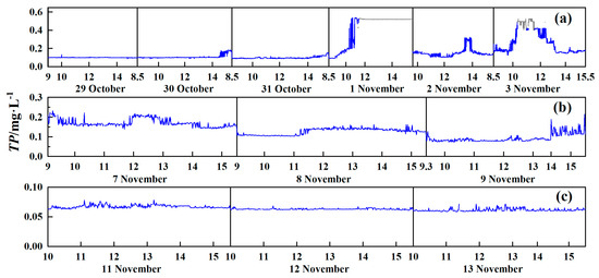
Figure 3.
Time series of TP derived from the GHPSs and XGboost TP estimation model in Lake Taihu (a) from 29 October to 3 November 2020; Liangxi River (b) during 7–9 November 2020 and Fuchunjiang Reservoir (c) during 11–13 November 2020. Note the data of the grey represent the abnormal data with NDVI values above 0.4, which are not used for statistics and calculation.
In general, the time series of TP in LT recorded the most dramatic variation which could be roughly divided into a low-value stable period with a mean value of 0.10 ± 0.01 mg·L−1 from 29 to 31 October and a sharp change period with a range of 0.09 to 0.54 mg·L−1 and a mean value of 0.19 ± 0.09 mg·L−1 from 1 to 3 November (Figure 3a). The TP of the second stage was significantly higher than that of the first stage (nonparametric test, p < 0.05), illustrating the water quality had deteriorated. For the second stage, there were three drastic variations in TP. Fundamentally, the TP increased exponentially from 0.10 mg·L−1 at 8:30 to 0.54 mg·L−1 at 10:40 on 1 November, increasing by 440.0% (R2 = 0.65, p < 0.05). Additionally, a complete single peak of TP was captured on 2 November, which quickly increased from 0.16 mg·L−1 at 13:25 to the peak value of 0.32 mg·L−1 at 13:50, then decreased to 0.15 mg·L−1 at 14:15. The last variation in TP concentration was observed on 3 November, when it quickly increased from 0.17 mg·L−1 at 9:51 to the first peak value of 0.42 mg·L−1 at 10:19, and then decreased to a low value of 0.15 mg·L−1 at 13:19.
Subsequently, TP decreased significantly from 7 to 9 November (R2 = 0.57, p < 0.01) with mean values of 0.17 ± 0.02 mg·L−1, 0.13 ± 0.02 mg·L−1 and 0.091 ± 0.02 mg·L−1 in LR (Figure 3b), implying that the nutrient load of LR decreased day by day, consistently with laboratory analysis. Furthermore, it should be noted that two short-term rapid rise events for TP occurred: from 0.16 mg·L−1 at 11:48 to 0.22 mg·L−1 at 12:03 on 7 November, or an increase of 37.5%, as well as an increase from 0.08 mg·L−1 at 13:34 to 0.19 mg·L−1 at 14:13 on 9 November, or an increase of 137.5%, indicating that the water body had experienced two pollution events recorded by the GHPSs.
In contrast to LR and LT, the TP of FR had no obvious diurnal variation from 11 to 13 November with mean values of 0.07 ± 0.003 mg·L−1, 0.06 ± 0.001 mg·L−1 and 0.06 ± 0.002 mg·L−1 respectively, revealing the relative stability of nutrient load in FR (Figure 3c).
4. Discussion
4.1. Reliability and Stability of the GHPSs Spectrum Data under Complex Weather
Acquiring accurate water-leaving radiation data is the basis of remote sensing of water quality [51,52]. For satellite remote sensing, radiometric calibration, cloud mask and atmospheric correction are widely performed to acquire accurate spectrum data [53]. As innovative monitoring equipment, the reliability and stability of the GHPSs spectra for TP estimation need to be discussed with reference to the synchronous measured Rrs(λ), especially under complex weather. Therefore, a linear regression analysis on each R(λ) and the synchronous measured Rrs(λ) from 400 nm to 900 nm was conducted. Significantly strong correlations with R2 of more than 0.99 (p < 0.01) were found in 20 pairs of matching datasets, which implied that the spectral shapes between R(λ) and Rrs(λ) were highly consistent under complex weather conditions (Figure S1 in Supporting Information). However, the extent and regression analysis slopes (a range of 2.3 to 4.8) between Rrs(λ) and R(λ) showed obvious differences. In other words, different extents indicated different light intensities, and different slopes meant that the response relationship between Rrs(λ) and R(λ) was unstable under different light intensities, which would result in great deviation in estimating the same water body under different weather conditions. Therefore, considering highly consistent spectral shapes and different slopes between Rrs(λ) and R(λ), we first proposed the maxima standardized method to eliminate the inconsistencies caused by complex weather without changing spectral shapes. In this method, the maximum bands with the highest frequency were counted as the reference band, the corrected spectrum data was the ratio of each band to the reference band. To evaluate the stability of the corrected spectrum under different weather, 574 nm with the highest frequency of the maximum spectral value in 20 spectral curves was selected as the standardized reference band under complex weather. Then, linear regression between the standardized Rrs(λ) and R(λ) was carried out, which yielded a fitting line with the slope and R2 values of 0.98 and 0.99, respectively (n = 10,521, p < 0.05) (Figure 4b), which were better than those before standardization (Figure 4a). In simpler terms, the results between the standardized R(λ) and Rrs(λ) along a 1:1 line meant that their response relationship is consistent and stable in complex weather, which improved the accuracy of the GHPSs spectrum. The maxima standardized method offset the error before and after standardization, which further enhanced the robustness and accuracy of the TP model in sunny, cloudy, and overcast weather.
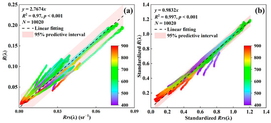
Figure 4.
Linear regression between Rrs(λ) and R(λ) from 400 to 900 nm before (a) and after (b).
4.2. Advantages of the Real-Time Tracking of TP Using GHPSs
With the rapid development of agricultural modernization and urbanization, massive amounts of phosphorus have been discharged and enriched into ditches, rivers, lakes and reservoirs, resulting in water quality deterioration and eutrophication since the 1980s [6,12,54,55]. However, time-consuming and spatiotemporal limited manual sampling methods, weather-vulnerable satellite and UAV remote sensing methods, and underwater sensors being limited by adhesive fouling, have resulted in the requirements for rapid, timely, accurate and reliable TP monitoring not being met [15]. Fortunately, with the development of sensor technology and the advent of the era of big data, the GHPSs with automation, real-time online, visualization and commercialization have overcome these shortcomings [56,57,58,59]. Unlike the existing traditional methods, the GHPSs, with characteristics of simple and efficient, high spectral and temporal-spatial resolution as well as proximal sensing, realized unmanned, real-time online, high-frequency, accurate and continuous observation of TP under complex weather, not only validates and supplements the TP dataset collected by traditional methods but also quickly diagnoses sudden TP pollution events, effectively improving regulatory capacity and service quality. Overall, the advantages of TP monitoring using the GHPSs are as follows:
First, the GHPSs provides an efficient and easy-operation tool for rapid observation of TP dynamics without secondary pollution under normal temperature and pressure. The traditional laboratory analysis method and automatic analyzer for TP needed to go through, not only cockamamie sampling, reaction reagent addition and spectrophotometer measurement, but also high temperature and high-pressure digestion, which slowed down the monitoring efficiency and caused thermal pollution and secondary chemical pollution to the natural water body [19,60]. Similarly, extracting TP from satellite and UAVs images also requires complex radiometric calibration, atmospheric correction, geometric correction and model development and application [18,28,50], all of which require not only high knowledge reserves but also professional skills. These defects were the current challenges in rapid monitoring of TP, which urgently needed to be solved [60]. In contrast, real-time TP derived from the GHPSs was exhibited on the terminal by simply setting the sampling frequency under normal temperature and pressure without secondary pollution, which improved monitoring efficiency and lowered barriers to entry for TP inspectors.
Second, using the GHPSs for real-time, high-frequency and continuous TP observation was conducive to tracking complete variation, and validating and supplementing the dataset collected by traditional monitoring methods. Under the superimposed influence of anthropogenic activities and extreme weather, the response of the TP loads in rivers and lakes to precipitation, plume and wind waves varied significantly with time on a daily scale [28,61]. Whereas, low-frequency manual sampling and satellite remote sensing with a fixed revisit, limited the operation time, and possible cloud obscuration resulted in data gaps for TP (TP can only be recorded during cloudless observation times), which might distort the pattern of TP [62]. Figure 5a displays the time and cloud conditions of the Moderate Resolution Imaging Spectroradiometer (MODIS, square) and Geostationary Ocean Color Imager (GOCI, triangle) crossing LT from 29 October to 3 November 2020. The green and blue colors represent cloudless while the black represents the cloud covering LT. The effective cloudless images of MODIS and GOCI were less than 50% during the observation period (Figure 5a). Moreover, Figure 5b shows the distribution of the monthly cloudless MODIS image covering LT during 2003–2020. About 70.8% of the months had less than 10 effective images and 96.8% of the months had less than 15 effective images. Therefore, the lack of enormous image data caused by cloud and a fixed revisit time was an important reason that hinders the continuous recording of the water environment by satellites. Although the UAVs performed proximal sensing to reduce the impact of aerosols and cloud, the limited hover time still limited its continuous TP observation. In contrast, the applicability to complex weather, proximal sensing avoided the effect of cloud, as well as an uninterruptible power supply, provided the possibility for the GHPSs recording high-frequency observation of total phosphorus, further created conditions for multi-temporal satellite data verification and supplements. In Figure 5a, the minute scale TP dataset derived from GHPSs supplemented the lack of satellite data and completely depicted an exponential increase and two complete single peak variations for TP during 1–3 November.

Figure 5.
The time and cloud conditions of MODIS and GOCI images covering Lake Taihu from 29 October to 3 November 2020 (a) and the distribution of monthly cloud-free high-quality MODIS images covering Lake Taihu from 2003 to 2020 (b).
Last but not the least, the GHPSs with proximal and non-contact sensing improved the accuracy and reliability of TP estimation. Less than 10% of the effective water signal is received by satellite and difficult atmospheric correction directly impacts the accuracy of the TP estimation [52]. Although the underwater sensor was not limited by the atmosphere, its application was affected by cost, and it is easy to be eroded by wind and waves, and there is significant data error caused by adhesive pollution [21,60,63]. Fortunately, the 4–5 m observation height of the GHPSs not only reduced the influence of atmospheric aerosols and increased the signal-to-noise ratio of the water body, but also avoided wind-wave erosion and adhesive pollution, which improved the accuracy of spectrum data for TP estimation.
Although the GHPSs has successfully estimated TP in LT, LR and FR, it still faces some improvements in precision and application, mainly in the following three aspects. First, the observation field needs to be expanded from point to plane because the single-point spectrometer limits the observation field of the GHPSs. Second, more water samples with complex optical characteristics are required for developing the TP estimation model, because the representativeness, universality and diversity of water quality datasets directly influence the stability and robustness of the proximal sensing models. Third, more estimation methods such as analytical, semi-analytical models, and even deep learning will be introduced to develop an intelligent TP estimation model.
4.3. Potential Application and Significance of Water Quality Monitoring Using the GHPSs
With the increasingly prominent problem of global water eutrophication and cyanobacterial blooms, governments have paid extensive attention and strengthened the management of pollution control, environmental treatment and aquatic ecosystem restoration, but the problem remains serious [2,64]. For instance, a total of 337,000 tons of TP were discharged into the water in China in 2020, 73.5% from agriculture, 1.1% from industry and 25.4% from domestic sewage (https://www.mee.gov.cn/hjzl/sthjzk/sthjtjnb/202202/W020220218339925977248.pdf (accessed on 18 February 2022)). Therefore, it is urgent to strengthen the rapid, timely, accurate, reliable, and cost-effective monitoring and management of surface water, which provides an opportunity for the GHPSs with real-time high-frequency and suitability for complex weather.
Lakes and rivers are highly dynamic and heterogeneous systems, which are sensitive to anthropogenic perturbations, hydrology, and meteorological changes [65]. It is a great challenge to capture the temporal and spatial variation pattern of water quality with one type of monitoring equipment [66,67]. Therefore, it is necessary to cooperate with a variety of monitoring equipment to establish an integrated “space-air-ground” multi-platform observation network. Deeply integrating the advantages of high-precision manual sampling, large-scale satellite remote sensing, the mobility and flexibility of the UAV, as well as the real-time high-frequency and continuity of the GHPSs overcome the defects of one type of monitoring equipment and realizes the real-time perception of multi-temporal and spatial scales and multi-parameter water quality [27,67,68]. Finally, a real-time dynamic water quality database is generated to serve the environmental management department. As an important part of the integrated multi-platform observation network of the water environment in the future, the GHPSs has been deployed in 13 rivers and reservoirs, such as LT (Jiangsu Province), Ganjiang River (Jiangxi Province) and Qiandao Lake (Zhejiang Province), initially forming a ground joint observation network (Figure S2).
In addition, the GHPSs, with the characteristics of accurate, real-time online, minute-scale sampling frequency and the efficient identification of abnormal data stands out for use in the emergency monitoring and early warning system in the face of sudden water environmental pollution events (Figure 3 and Figure 6). In the future, relying on the high spatial-temporal resolution, multi-dimensional and real-time water quality database collected by the integrated “space-air-ground” multi-platform observation network, a watershed emergency management system will be established. It aims to quickly identify water quality abnormalities, timely diagnose sudden water events, automatically alarm and start emergency plans, and release real-time water quality dynamics, which help coordinate regional joint prevention and linkage, clarify regional pollution responsibilities, and form a scientific and perfect water emergency prevention and control system. At the same time, the accurate and high-frequency water quality database provides data support for short-term prediction and early warning, improving the accuracy and timeliness of early warning and diagnosis. Therefore, the GHPSs will become an indispensable part of emergency early warning and monitoring systems in the future and has broad application prospects.
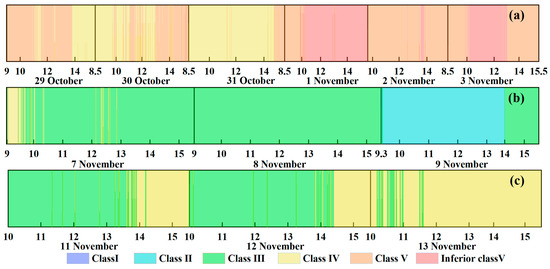
Figure 6.
Time series of water body types of Lake Taihu (a), Liangxi River (b) and Fuchunjiang Reservoir (c) based on total phosphorus concentration assessment from 9:00 to 15:30 during 29 October to 13 November 2020.
5. Conclusions
In this study, a real-time high-frequency and automatic GHPSs is proposed for tracking TP dynamics, which is characterized by a spectral resolution of 1 nm between 400 nm and 900 nm and a minimum sampling interval of 20 s. A TP machine learning model was developed and validated with ideal accuracy based on the XGBoost method using 377 pairs of synchronous samples (R2 = 0.97, RMSE = 0.017 mg·L−1, MAPE = 12.8%). Compared with traditional TP monitoring equipment, the GHPSs, with the advantages of simple operation, high-frequency, real-time, accurate and being suitable for complex weather, supplements the defects of low frequency monitoring, poor timeliness and accuracy of existing monitoring equipment, and complements the lack of TP data during overcast and cloudy weather. Short and rapid TP changes were observed within one day in LT and LR based on the GHPSs minute scale monitoring, which highlighted the importance of high frequency observation of TP. In the future, the GHPSs has great potential value and application prospects in raising our awareness of the dynamics and driving mechanisms of water quality for inland waters. Therefore, our findings will contribute to the deep understanding of short-term dynamics and long-term trends of TP concentration by using the GHPSs, which will greatly improve water environment management and prediction precision for algal blooms.
Supplementary Materials
The following supporting information can be downloaded at https://www.mdpi.com/article/10.3390/rs15020507/s1: Figure S1. The relationship between R(λ) and corresponding Rrs(λ) from 400 to 900 nm under overcast (a–e), cloud (f–i) and sunny (m–t); Figure S2. The application of GHPSs in different water bodies including Lake Taihu (a), Ganjiang River (b), an urban lake in shanghai (c), Daxi Reservoir (d), Fuchunjiang Reservoir (e), Liangxi River (f), Juhe River (g), Chenhe River (h) and Shiwei River (i).
Author Contributions
Investigation, data curation, software, visualization, methodology, writing and editing, N.L.; conceptualization, supervision, writing and editing, Y.Z. (Yunlin Zhang); resources, writing and editing, funding acquisition, K.S.; software, investigation, Y.Z. (Yibo Zhang); investigation and data curation X.S., W.W., H.Q., H.Y., Y.N. All authors have read and agreed to the published version of the manuscript.
Funding
This study was funded by the Special Program of Network Security and Informatization of Chinese Academy of Sciences (CAS-WX2021SF-0504), the Industry Prospect and Key Core Technology Project of Jiangsu Province (BE2022152), the Scientific Instrument Developing Project of the Chinese Academy of Sciences (YJKYYQ20200071), Social Development Foundation of Jiangsu province (BE2022857), Water Resource Science and Technology Project in Jiangsu Province (2020004 and 2020057), the Tibetan Plateau Scientific Expedition and Research Program (2019QZKK0202), and the NIGLAS foundation (E1SL002). We are grateful to all participants for their contribution in the field investigation. We would like to express our gratitude to the three anonymous reviewers for their critical comments and constructive suggestions.
Data Availability Statement
The data presented in this study are available on request from the corresponding author.
Conflicts of Interest
The authors declare no conflict of interest.
References
- Howarth, R.W.; Marino, R. Nitrogen as the limiting nutrient for eutrophication in coastal marine ecosystems: Evolving views over three decades. Limnol. Oceanogr. 2006, 51, 364–376. [Google Scholar] [CrossRef]
- Powers, S.M.; Bruulsema, T.W.; Burt, T.P.; Chan, N.I.; Elser, J.J.; Haygarth, P.M.; Howden, N.J.K.; Jarvie, H.P.; Lyu, Y.; Peterson, H.M.; et al. Long-term accumulation and transport of anthropogenic phosphorus in three river basins. Nat. Geosci. 2016, 9, 353–356. [Google Scholar] [CrossRef]
- Stow, C.A.; Cha, Y.; Johnson, L.T.; Confesor, R.; Richards, R.P. Long-term and seasonal trend decomposition of Maumee River nutrient inputs to western Lake Erie. Environ. Sci. Technol. 2015, 49, 3392–3400. [Google Scholar] [CrossRef]
- Schindler, D.W.; Hecky, R.E.; Findlay, D.L.; Stainton, M.P.; Parker, B.R.; Paterson, M.J.; Beaty, K.G.; Lyng, M.; Kasian, S.E.M. Eutrophication of lakes cannot be controlled by reducing nitrogen input: Results of a 37-year whole-ecosystem experiment. Proc. Natl. Acad. Sci. USA 2008, 105, 11254–11258. [Google Scholar] [CrossRef]
- Carpenter, S.R. Phosphorus control is critical to mitigating eutrophication. Proc. Natl. Acad. Sci. USA 2008, 105, 11039–11040. [Google Scholar] [CrossRef]
- Sinha, E.; Michalak, A.M.; Balaji, V. Eutrophication will increas during the 21st century as a result of precipitation changes. Sccience 2017, 357, 405–408. [Google Scholar] [CrossRef]
- Ho, J.C.; Michalak, A.M.; Pahlevan, N. Widespread global increase in intense lake phytoplankton blooms since the 1980s. Nature 2019, 574, 667–670. [Google Scholar] [CrossRef]
- Wang, S.; Li, J.; Zhang, B.; Spyrakos, E.; Tyler, A.N.; Shen, Q.; Zhang, F.; Kuster, T.; Lehmann, M.K.; Wu, Y.; et al. Trophic state assessment of global inland waters using a MODIS-derived Forel-Ule index. Remote Sens. Environ. 2018, 217, 444–460. [Google Scholar] [CrossRef]
- Abell, J.M.; Ozkundakci, D.; Hamilton, D.P.; van Dam-Bates, P.; McDowell, R.W. Quantifying the extent of anthropogenic eutrophication of lakes at a national scale in New Zealand. Environ. Sci. Technol. 2019, 53, 9439–9452. [Google Scholar] [CrossRef]
- Hussain, T.S.; Al-Fatlawi, A.H. Remove chemical contaminants from potable water by household water treatment system. Civ. Eng. J. 2020, 6, 1534–1546. [Google Scholar] [CrossRef]
- Zhang, Y.; Deng, J.; Qin, B.; Zhu, G.; Zhang, Y.; Jeppesen, E.; Tong, Y. Importance and vulnerability of lakes and reservoirs supporting drinking water in China. Fundam. Res. 2022, Online. [Google Scholar] [CrossRef]
- Hou, X.; Feng, L.; Dai, Y.; Hu, C.; Gibson, L.; Tang, J.; Lee, Z.; Wang, Y.; Cai, X.; Liu, J.; et al. Global mapping reveals increase in lacustrine algal blooms over the past decade. Nat. Geosci. 2022, 15, 130–134. [Google Scholar] [CrossRef]
- Nkansah, M.A.; Donkoh, M.; Akoto, O.; Ephraim, J.H. Preliminary studies on the use of sawdust and peanut shell powder as adsorbents for phosphorus removal from water. Emerg. Sci. J. 2019, 3, 33. [Google Scholar] [CrossRef]
- Xiong, J.; Lin, C.; Cao, Z.; Hu, M.; Xue, K.; Chen, X.; Ma, R. Development of remote sensing algorithm for total phosphorus concentration in eutrophic lakes: Conventional or machine learning? Water Res. 2022, 215, 118213. [Google Scholar] [CrossRef] [PubMed]
- Wang, G.; Li, J.; Sun, W.; Xue, B.; Yinglan, A.; Liu, T. Non-point source pollution risks in a drinking water protection zone based on remote sensing data embedded within a nutrient budget model. Water Res. 2019, 157, 238–246. [Google Scholar] [CrossRef]
- Zhuang, Y.; Wen, W.; Ruan, S.; Zhuang, F.; Xia, B.; Li, S.; Liu, H.; Du, Y.; Zhang, L. Real-time measurement of total nitrogen for agricultural runoff based on multiparameter sensors and intelligent algorithms. Water Res. 2022, 210, 117992. [Google Scholar] [CrossRef]
- Du, C.; Li, Y.; Lyu, H.; Liu, N.; Zheng, Z.; Li, Y. Remote estimation of total phosphorus concentration in the Taihu Lake using a semi-analytical model. Int. J. Remote Sens. 2020, 41, 7993–8013. [Google Scholar] [CrossRef]
- Du, C.; Wang, Q.; Li, Y.; Lyu, H.; Zhu, L.; Zheng, Z.; Wen, S.; Liu, G.; Guo, Y. Estimation of total phosphorus concentration using a water classification method in inland water. Int. J. Appl. Earth Obs. Geoinf. 2018, 71, 29–42. [Google Scholar] [CrossRef]
- Xu, J.; Lin, K.; Huang, Y.; Guo, Q.; Li, H.; Yuan, D. Development of an online analyzer for determination of total phosphorus in industrial circulating cooling water with UV photooxidation digestion and spectrophotometric detection. Talanta 2019, 201, 74–81. [Google Scholar] [CrossRef]
- Li, C.; Wang, B.; Wan, H.; He, R.; Li, Q.; Yang, S.; Dai, W.; Wang, N. An integrated optofluidic platform enabling total phosphorus on-chip digestion and online real-time detection. Micromachines 2020, 11, 59. [Google Scholar] [CrossRef]
- Chen, Y.T.; Crossman, J. The impacts of biofouling on automated phosphorus analysers during long-term deployment. Sci. Total Environ. 2021, 784, 147188. [Google Scholar] [CrossRef] [PubMed]
- Viviano, G.; Salerno, F.; Manfredi, E.C.; Polesello, S.; Valsecchi, S.; Tartari, G. Surrogate measures for providing high frequency estimates of total phosphorus concentrations in urban watersheds. Water Res. 2014, 64, 265–277. [Google Scholar] [CrossRef] [PubMed]
- Olson, C.R.; Jones, S.E. Chlorophyll–total phosphorus relationships emerge from multiscale interactions from algae to catchments. Limnol. Oceanogr. Lett. 2022, 7, 483–491. [Google Scholar] [CrossRef]
- Zhang, Y.; Zhou, Y.; Shi, K.; Qin, B.; Yao, X.; Zhang, Y. Optical properties and composition changes in chromophoric dissolved organic matter along trophic gradients: Implications for monitoring and assessing lake eutrophication. Water Res. 2018, 131, 255–263. [Google Scholar] [CrossRef]
- Zhang, Y.; Shi, K.; Zhou, Y.; Liu, X.; Qin, B. Monitoring the river plume induced by heavy rainfall events in large, shallow, Lake Taihu using MODIS 250m imagery. Remote Sens. Environ. 2016, 173, 109–121. [Google Scholar] [CrossRef]
- Zhou, Y.; Liu, M.; Zhou, L.; Jang, K.S.; Xu, H.; Shi, K.; Zhu, G.; Liu, M.; Deng, J.; Zhang, Y.; et al. Rainstorm events shift the molecular composition and export of dissolved organic matter in a large drinking water reservoir in China: High frequency buoys and field observations. Water Res. 2020, 187, 116471. [Google Scholar] [CrossRef]
- Li, N.; Zhang, Y.; Shi, K.; Zhang, Y.; Sun, X.; Wang, W.; Huang, X. Monitoring water transparency, total suspended matter and the beam attenuation coefficient in inland water using innovative ground-based proximal sensing technology. J. Environ. Manag. 2022, 306, 114477. [Google Scholar] [CrossRef]
- Du, C.; Li, Y.; Wang, Q.; Liu, G.; Zheng, Z.; Mu, M.; Li, Y. Tempo-spatial dynamics of water quality and its response to river flow in estuary of Taihu Lake based on GOCI imagery. Environ. Sci. Pollut. Res. 2017, 24, 28079–28101. [Google Scholar] [CrossRef]
- Song, K.; Brewer, A.; Ahmadian, S.; Shankar, A.; Detweiler, C.; Burgin, A.J. Using unmanned aerial vehicles to sample aquatic ecosystems. Limnol. Oceanogr. Methods 2017, 15, 1021–1030. [Google Scholar] [CrossRef]
- Qin, B.; Zhu, G.; Gao, G.; Zhang, Y.; Li, W.; Paerl, H.W.; Carmichael, W.W. A drinking water crisis in Lake Taihu, China: Linkage to climatic variability and lake management. Environ. Manag. 2010, 45, 105–112. [Google Scholar] [CrossRef]
- Zhang, M.; Duan, H.; Shi, X.; Yu, Y.; Kong, F. Contributions of meteorology to the phenology of cyanobacterial blooms: Implications for future climate change. Water Res. 2012, 46, 442–452. [Google Scholar] [CrossRef]
- Qin, B.; Deng, J.; Shi, K.; Wang, J.; Brookes, J.; Zhou, J.; Zhang, Y.; Zhu, G.; Paerl, H.W.; Wu, L. Extreme climate anomalies enhancing cyanobacterial blooms in eutrophic Lake Taihu, China. Water Resour. Res. 2021, 57, e2020WR029371. [Google Scholar] [CrossRef]
- He, X.; Wang, H.; Yan, H.; Ao, Y. Numerical simulation of microcystin distribution in Liangxi River, downstream of Taihu Lake. Water Environ. Res. 2020, 93, 1934–1943. [Google Scholar] [CrossRef]
- Feng, L.; Sun, X.; Zhu, X. Impact of floodgates operation on water environment using one-dimensional modelling system in river network of Wuxi city, China. Ecol. Eng. 2016, 91, 173–182. [Google Scholar] [CrossRef]
- Guo, Y.; Xu, H.; Chen, X.; Zheng, J.; Zhan, X.; Zhu, G.; Zhu, M. Change of algal particles and its water quality effect in the outflow river of Taihu Lake. Environ. Sci. 2021, 42, 242–250. [Google Scholar] [CrossRef]
- Wu, T.; Luo, L.; Qin, B.; Cui, G.; Yu, Z.; Yao, Z. A vertically integrated eutrophication model and its application to a river-style reservoir—Fuchunjiang, China. J. Environ. Sci. 2009, 21, 319–327. [Google Scholar] [CrossRef]
- Qunfang, H.; Chaoxuan, G.; Na, L.; Yuan, L. Characteristics of summer heat waves and potential effect on algal blooms in Fuchunjiang Reservoir. Res. Environ. Sci. 2022, 35, 530–539. [Google Scholar] [CrossRef]
- Guo, C.; Zhu, G.; Paerl, H.W.; Zhu, M.; Yu, L.; Zhang, Y.; Liu, M.; Zhang, Y.; Qin, B. Extreme weather event may induce microcystis blooms in the Qiantang River, Southeast China. Environ. Sci. Pollut. Res. 2018, 25, 22273–22284. [Google Scholar] [CrossRef]
- Simis, S.G.H.; Peters, S.W.M.; Gons, H.J. Remote sensing of the cyanobacterial pigment phycocyanin in turbid inland water. Limnol. Oceanogr. 2005, 50, 237–245. [Google Scholar] [CrossRef]
- Xiong, J.; Lin, C.; Ma, R.; Cao, Z. Remote sensing estimation of lake total phosphorus concentration based on MODIS: A case study of Lake Hongze. Remote Sens. 2019, 11, 2068. [Google Scholar] [CrossRef]
- Tang, J.; Tian, G.; Wang, X.; Wang, X.; Song, Q. The methods of water spectra measurement and analysis Ⅰ: Above-water method. J. Remote Sens. 2004, 8, 37–44. [Google Scholar] [CrossRef]
- Zhang, Y.; Zhang, Y.; Shi, K.; Zhou, Y.; Li, N. Remote sensing estimation of water clarity for various lakes in China. Water Res. 2021, 192, 116844. [Google Scholar] [CrossRef] [PubMed]
- Li, N.; Shi, K.; Zhang, Y.; Gong, Z.; Peng, K.; Zhang, Y.; Zha, Y. Decline in transparency of Lake Hongze from long-term MODIS observations: Possible causes and potential significance. Remote Sens. 2019, 11, 177. [Google Scholar] [CrossRef]
- Sun, X.; Zhang, Y.; Shi, K.; Zhang, Y.; Li, N.; Wang, W.; Huang, X.; Qin, B. Monitoring water quality using proximal remote sensing technology. Sci. Total Environ. 2022, 803, 149805. [Google Scholar] [CrossRef]
- Chang, N.-B.; Xuan, Z.; Yang, Y.J. Exploring spatiotemporal patterns of phosphorus concentrations in a coastal bay with MODIS images and machine learning models. Remote Sens. Environ. 2013, 134, 100–110. [Google Scholar] [CrossRef]
- Gao, Y.; Gao, J.; Yin, H.; Liu, C.; Xia, T.; Wang, J.; Huang, Q. Remote sensing estimation of the total phosphorus concentration in a large lake using band combinations and regional multivariate statistical modeling techniques. J. Environ. Manag. 2015, 151, 33–43. [Google Scholar] [CrossRef]
- Shi, K.; Zhang, Y.; Zhou, Y.; Liu, X.; Zhu, G.; Qin, B.; Gao, G. Long-term MODIS observations of cyanobacterial dynamics in Lake Taihu: Responses to nutrient enrichment and meteorological factors. Sci. Rep. 2017, 7, 40326. [Google Scholar] [CrossRef]
- Chen, T.; He, T.; Benest, Y.M.; Khotilovic, H.V.; Tang, Y.; Cho, H.; Chen, K. Xgboost: Extreme gradient boosting. R Package Version 0.4-2 2015, 1, 1–4. Available online: https://www.bibsonomy.org/bibtex/23ab0146e17e289054647d77c16c383e3/msteininger (accessed on 12 January 2023).
- Zhang, Y.; Shi, K.; Sun, X.; Zhang, Y.; Li, N.; Wang, W.; Zhou, Y.; Zhi, W.; Liu, M.; Li, Y.; et al. Improving remote sensing estimation of Secchi disk depth for global lakes and reservoirs using machine learning methods. GIScience Remote Sens. 2022, 59, 1367–1383. [Google Scholar] [CrossRef]
- Tian, S.; Guo, H.; Xu, W.; Zhu, X.; Wang, B.; Zeng, Q.; Mai, Y.; Huang, J.J. Remote sensing retrieval of inland water quality parameters using Sentinel-2 and multiple machine learning algorithms. Environ. Sci. Pollut. Res. 2022. [Google Scholar] [CrossRef]
- Wang, M.; Shi, W. The NIR-SWIR combined atmospheric correction approach for MODIS ocean color data processing. Opt. Express 2007, 15, 15722–15733. [Google Scholar] [CrossRef] [PubMed]
- Surisetty, V.V.A.K.; Sahay, A.; Ramakrishnan, R.; Samal, R.N.; Rajawat, A.S. Improved turbidity estimates in complex inland waters using combined NIR–SWIR atmospheric correction approach for Landsat 8 OLI data. Int. J. Remote Sens. 2018, 39, 7463–7482. [Google Scholar] [CrossRef]
- Liu, G.; Li, Y.; Lyu, H.; Wang, S.; Du, C.; Huang, C. An improved land target-based atmospheric correction method for Lake Taihu. IEEE J. Sel. Top. Appl. Earth Obs. Remote Sens. 2016, 9, 793–803. [Google Scholar] [CrossRef]
- Xu, H.; Qin, B.; Paerl, H.W.; Peng, K.; Zhang, Q.; Zhu, G.; Zhang, Y. Environmental controls of harmful cyanobacterial blooms in Chinese inland waters. Harmful Algae 2021, 110, 102127. [Google Scholar] [CrossRef]
- Gao, Y.; Zhou, F.; Ciais, P.; Miao, C.; Yang, T.; Jia, Y.; Zhou, X.; Klaus, B.-B.; Yang, T.; Yu, G. Human activities aggravate nitrogen-deposition pollution to inland water over China. Natl. Sci. Rev. 2020, 7, 430–440. [Google Scholar] [CrossRef]
- Ye, L.; Cai, Q.; Zhang, M.; Tan, L. Real-time observation, early warning and forecasting phytoplankton blooms by integrating in situ automated online sondes and hybrid evolutionary algorithms. Ecol. Inform. 2014, 22, 44–51. [Google Scholar] [CrossRef]
- Teta, R.; Romano, V.; Sala, G.D.; Picchio, S.; Sterlich, C.D.; Mangoni, A.; Tullio, G.D.; Costantino, V.; Lega, M. Cyanobacteria as indicators of water quality in Campania coasts, Italy: A monitoring strategy combining remote/proximal sensing and in situ data. Environ. Res. Lett. 2017, 12, 024001. [Google Scholar] [CrossRef]
- Chang, N.B.; Bai, K.; Chen, C.F. Integrating multisensor satellite data merging and image reconstruction in support of machine learning for better water quality management. J. Environ. Manag. 2017, 201, 227–240. [Google Scholar] [CrossRef]
- Pomati, F.; Jokela, J.; Simona, M.; Veronesi, M.; Ibelings, B.W. An automated platform for phytoplankton ecology and aquatic ecosystem monitoring. Environ. Sci. Technol. 2011, 45, 9658–9665. [Google Scholar] [CrossRef]
- Zhou, X.; Cheng, W. Research progress of total phosphorus detection in water. Chem. Manag. 2021, 36, 148–149. [Google Scholar] [CrossRef]
- Shi, K.; Zhang, Y.; Zhang, Y.; Qin, B.; Zhu, G. Understanding the long-term trend of particulate phosphorus in a cyanobacteria-dominated lake using MODIS-Aqua observations. Sci. Total Environ. 2020, 737, 139736. [Google Scholar] [CrossRef]
- Marce, R.; George, G.; Buscarinu, P.; Deidda, M.; Dunalska, J.; de Eyto, E.; Flaim, G.; Grossart, H.P.; Istvanovics, V.; Lenhardt, M.; et al. Automatic high frequency monitoring for improved lake and reservoir management. Environ. Sci. Technol. 2016, 50, 10780–10794. [Google Scholar] [CrossRef] [PubMed]
- Cao, W.; Sun, Z.; Li, C.; Zou, G. Biofouling protection for water quality monitoring buoy and sensors. J. Trop. Oceanogr. 2018, 37, 7–12. [Google Scholar] [CrossRef]
- Deng, C.; Liu, L.; Peng, D.; Li, H.; Zhao, Z.; Lyu, C.; Zhang, Z. Net anthropogenic nitrogen and phosphorus inputs in the Yangtze River economic belt: Spatiotemporal dynamics, attribution analysis, and diversity management. J. Hydrol. 2021, 597, 126221. [Google Scholar] [CrossRef]
- Peng, Z.; Hu, W.; Liu, G.; Zhang, H.; Gao, R.; Wei, W. Development and evaluation of a real-time forecasting framework for daily water quality forecasts for Lake Chaohu to Lead time of six days. Sci. Total Environ. 2019, 687, 218–231. [Google Scholar] [CrossRef] [PubMed]
- Gittins, J.R.; Hemingway, J.R.; Dajka, J.C. How a water-resources crisis highlights social-ecological disconnects. Water Res. 2021, 194, 116937. [Google Scholar] [CrossRef] [PubMed]
- Duan, H.; Wan, N.; Qiu, Y.; Liu, G.; Chen, Q.; Luo, J.; Chen, Y.; Qi, T. Discussions and practices on the framework of monitoring system in eutrophic lakes and reservoirs. J. Lake Sci. 2020, 32, 1396–1405. [Google Scholar] [CrossRef]
- Qiu, Y.; Duan, H.; Wan, N.; Gao, R.; Huang, J.; Xun, K.; Peng, Z.; Xiao, P. Design and practice of a platform for monitoring, early-warning and simulation of algal blooms in Lake Chaohu. J. Lake Sci. 2022, 34, 38–48. [Google Scholar] [CrossRef]
Disclaimer/Publisher’s Note: The statements, opinions and data contained in all publications are solely those of the individual author(s) and contributor(s) and not of MDPI and/or the editor(s). MDPI and/or the editor(s) disclaim responsibility for any injury to people or property resulting from any ideas, methods, instructions or products referred to in the content. |
© 2023 by the authors. Licensee MDPI, Basel, Switzerland. This article is an open access article distributed under the terms and conditions of the Creative Commons Attribution (CC BY) license (https://creativecommons.org/licenses/by/4.0/).