A Handheld LiDAR-Based Semantic Automatic Segmentation Method for Complex Railroad Line Model Reconstruction

Abstract

To ensure efficient railroad operation and maintenance management, the accurate reconstruction of railroad BIM models is a crucial step. This paper proposes a workflow for automated segmentation and reconstruction of railroad structures using point cloud data, without relying on intensity or trajectory information. The workflow consists of four main components: point cloud adaptive denoising, scene segmentation, structure segmentation combined with deep learning, and model reconstruction. The proposed workflow was validated using two datasets with significant differences in railroad line point cloud data. The results demonstrated significant improvements in both efficiency and accuracy compared to existing methods. The techniques enable direct automated processing from raw data to segmentation results, providing data support for parameterized modeling and greatly reducing manual processing time. The proposed algorithms achieved an intersection over union (IoU) of over 0.9 for various structures in a 450-m-long railroad line. Furthermore, for single-track railroads, the automated segmentation time was within 1 min per kilometer, with an average mean intersection over union (MIoU) and accuracy of 0.9518 and 1.0000, respectively.

1. Introduction

Railroad systems have long been recognized as vital components of transportation networks, playing a crucial role in driving economic growth and facilitating social development [1,2,3]. However, the operation of railroads is susceptible to various factors such as geological changes, line degradation, and train-induced vibrations, which pose risks to their safe operation [4,5,6]. To ensure the stability and safety of railroads, it is essential to establish a real-time monitoring and maintenance system that replaces the conventional manual inspection methods, known for being inefficient and time-consuming [7].

The foundation of such a system lies in the railroad model, which serves as a platform for displaying diverse data. However, the complexity of railroad infrastructure, extensive track networks, and intricate structures make the reconstruction of accurate railroad models challenging and labor-intensive [8,9]. Therefore, there is a pressing need for digital construction techniques to efficiently capture and represent engineering structures. Moreover, as the demand for modifications and expansions continues to rise, exploring more efficient and precise management approaches becomes increasingly critical.

Digital construction not only facilitates subsequent maintenance and transformation processes by providing comprehensive data sources but also significantly enhances the efficiency of maintenance tasks while streamlining data collection and decision-making procedures [10,11,12].

With the advancement of technology, the combination of Building Information Modeling (BIM) and point cloud technology has found extensive applications in railroad maintenance and operations within the transportation sector [13,14,15]. By utilizing laser scanners to capture surface information of railroad infrastructure, a vast amount of precise three-dimensional point cloud data with coordinates and intensity information are obtained, facilitating the rapid and accurate reconstruction of large-scale BIM models [16,17,18]. This integration addresses various issues in railroad projects, such as incomplete drawing preservation, inaccuracies in construction descriptions, and variations during operational phases, which would otherwise hinder the precise establishment of BIM models [19,20,21]. Consequently, these issues lead to increased operational difficulties, rising costs, and reduced efficiency in information dissemination and scheduling [22,23].

The integration of BIM and point cloud technology provides the railroad engineering domain with digital twin systems that accelerate information sharing, enhance maintenance effectiveness, simulate scenarios, acquire health status information, and offer other advantages [24,25,26].

In the railroad domain, point cloud data collection is commonly achieved through the utilization of inspection vehicles mounted on the tracks [27,28]. However, such equipment is often associated with substantial costs and operational complexities as it necessitates running on the steel rails and requires obtaining approval for a “Skylight Period” from railroad operators. This approval process adds considerable difficulty to the scanning operation and results in significant maintenance expenses for railroad authorities.

In recent years, the adoption of Handheld LiDAR-based 3D point cloud acquisition methods has gained widespread acceptance and has been extensively validated for accuracy in various domains, including forestry, tunneling, mining, and urban environments [29,30]. These studies have demonstrated that Handheld LiDAR devices can provide data support with centimeter-level precision in large-scale scenes, proving instrumental in tasks such as visual positioning and model reconstruction.

One of the primary advantages of Handheld LiDAR-based devices is their relatively lower cost, enabling researchers to conduct data collection by walking and significantly reducing the barriers and expenses associated with scanning operations. However, it is important to note that, compared to the inspection vehicle-based scanning approach, the walking method presents challenges in accurately determining the alignment of railroad tracks based on trajectory information. This can potentially introduce data errors. Additionally, the intensity information of acquired points is influenced by various factors, such as scanning angles, target object characteristics, and equipment specifications, making it difficult to validate and account for errors during data processing in the railroad domain.

Addressing these challenges and advancements in Handheld LiDAR-based point cloud data acquisition holds promise for improving railroad maintenance and operational processes while optimizing costs and efficiency.

It is important to note that the vast amount of point cloud data generated by Lidar laser scanners lacks inherent structure and correlations, making it unsuitable for directly generating Building Information Modeling (BIM) models. Therefore, specific preprocessing is required to segment and extract necessary geometric information and feature representations from the acquired data [15,31]. This processing enables effective model reconstruction of railroad tracks, overhead lines, tunnels, bridges, and other structures [22,32,33].

Existing segmentation approaches in the railroad domain mostly rely on the trajectory and intensity information of railroad tracks, utilizing heuristic and hybrid model-fitting methods for extracting key structures [22,34]. However, these methods demonstrate limited effectiveness in complex point cloud scenes with significant structural variations, as they heavily depend on specific point cloud feature calculations for matching, resulting in reduced robustness. Any changes in the data or the influence of a considerable number of noise points may lead to deviations in the extracted results, rendering them ineffective, particularly when using Handheld LiDAR-based scanning devices. Thus, one crucial step in promoting the applicability and generalization of these segmentation methods is to reduce their dependence on specific data types and precision levels.

In recent years, the application of deep learning techniques [35] has gradually extended to feature extraction [36,37], classification, and segmentation [38,39,40,41,42] tasks for three-dimensional point cloud data, showcasing remarkable performance. Moreover, frameworks specifically tailored for point cloud data processing have matured [43,44,45]. However, there is currently a lack of publicly available segmentation datasets specifically designed for railroad scenes. Consequently, the absence of widely adopted segmentation algorithms has made the creation of railroad three-dimensional point cloud datasets a laborious process. Hence, there is an urgent need to drive the integration of deep learning with segmentation algorithms and develop suitable solutions for the automated segmentation of railroad point clouds. By addressing this challenge, the railroad industry can leverage the full potential of deep learning to enhance the efficiency and accuracy of point cloud segmentation, ultimately leading to more streamlined and automated workflows.

Following the segmentation of point cloud data, the data become structured. In subsequent project applications, it is advantageous to assign information to the structure first, facilitating data attachment in the comprehensive management system and establishing a one-to-one linkage with the model. Additionally, by leveraging parameterized point cloud data, the BIM model can be rapidly reconstructed, offering benefits such as reduced storage resource consumption, clear structural representation, and enhanced applicability compared to other methods [46].

The open image programming software Dynamo© [47], integrated into the Revit platform, enables programming input of linear structure parameters and direct modeling of the provided section. In this paper, the reconstruction of the railroad’s point cloud model primarily focuses on three key structures: tracks, power lines, and catenary posts, while also reconstructing the ground based on track information. Overall, the emphasis lies on linear structures and standard structures, aligning with the modeling characteristics supported by Dynamo©.

Building upon the aforementioned background, this paper presents a significant contribution in proposing an automated process for reconstructing railroad Building Information Modeling (BIM) models using Handheld LiDAR-based devices. The approach is designed to adapt to various railroad line Lidar three-dimensional laser point cloud coordinate data, without relying on trajectory information or intensity data. The key contributions of this research can be summarized as follows:

(1)

We introduce an automatic segmentation process for extracting key railroad structures from 3D point cloud coordinate data. This segmentation process does not rely on intensity information or scanning device trajectory information, ensuring its robustness and applicability;

(2)

We propose an adaptive filtering process and enhance the Cloth Simulation Filter (CSF) method to cater specifically to railroad scene point clouds. This enables the separation of ground and overhead line scenes and facilitates the rough extraction of rails;

(3)

We develop a rail point extraction algorithm that effectively handles noise and further refines the rail extraction process after the initial rough extraction;

(4)

We improve the hybrid machine learning-based power line extraction algorithm to significantly enhance extraction performance;

(5)

We combine deep learning techniques with segmentation algorithms to achieve the automatic segmentation of corresponding structures. Furthermore, we establish a BIM model by performing parameterized extraction of the structure.

2. Related Work

2.1. Semantic Segmentation of Key Railroad Structures

The segmentation of railroad point cloud data is often challenging due to the large volume and complex structure of the data, making manual division a time-consuming and labor-intensive task. However, the dominant structures in railroads are typically linear, such as tracks and power lines, which allows for segmentation by leveraging geometric features and corresponding algorithms.

Existing algorithms primarily rely on heuristic approaches and utilize external contour features and intensity information of rail tracks as the basis for segmentation. For instance, Sánchez-Rodríguez et al. [28] proposed a heuristic method that successfully segmented various parts of a railroad tunnel by exploiting the geometry features and intensity information of rail tracks. The method effectively extracted structures like the ground and tracks.

In a subsequent study, M. Soilán et al. [48] employed a heuristic point cloud processing step to reliably extract rail track point clouds. They detected linearity through equation fitting and converted the data into a format compliant with the Industry Foundation Classes (IFC) standard for BIM modeling. This approach successfully achieved the reconstruction of a BIM model from point cloud data. However, it should be noted that the effectiveness of this method decreases when applied to more complex scenes, such as multi-line tracks and other ground facilities.

The intensity information in point clouds is influenced by numerous factors, and more importantly, it is relative and can exhibit significant variations across different point cloud datasets [49]. Hence, it is advisable to minimize the reliance on intensity information during the point cloud segmentation process. On the other hand, the geometry information of steel rails remains relatively consistent, making the extraction of geometry information more stable and easier to verify and evaluate. Consequently, the crucial aspect of extracting steel rails from diverse point cloud data lies in effectively handling the ground information in different scenes.

Previous research, such as that conducted by Yun-Jian Cheng [22], successfully extracted track vertices from relatively flat tunnels using solely the height difference information of steel rails. The extracted line form was then employed for track model reconstruction. However, such methods become ineffective when confronted with more complex ground information. To the best of the author’s knowledge, there is currently no universal approach capable of accurately separating railroad tracks from ground surfaces in complex environments.

Existing ground filtering algorithms, such as morphological operations, normal differences, and region growing, lack theoretical support when addressing these challenges [50,51,52]. In recent years, progressively morphological filters (PMF) [53] and cloth simulation filters (CSF) [54], which are scale-invariant and terrain-adaptive, have been widely utilized in combination with irregular triangulated networks (TIN) or differential digital elevation models (DEM) [55,56,57] to process digital terrain models (DTM) obtained from airborne LiDAR. These methods often employ native techniques and integrate them with other approaches to separate the ground from large-scale scenes and extract structures like trees, buildings, and power lines. However, they typically have low requirements for detailed results. When faced with the separation of specific structures, such as railroad vegetation filtering and shield tunnel bolt-hole extraction [27,58], a higher level of detail is required, necessitating adaptive modifications to the CSF method. Despite these adaptations, these methods still primarily focus on extracting a particular type of outward protruding structure from the space, which demonstrates the versatility of the approach. Currently, there are no studies that have employed the CSF method for railroad structure extraction. Hence, there is value and rationale in enhancing the CSF method to suit the extraction of railroad structures.

In the segmentation of overhead line-type structures, a common approach is the adoption of a mixed model fitting method. Liang et al. utilized the least squares method (LSM) to identify power lines and reconstruct them based on the spatial distribution characteristics of adjacent point clouds [59]. Yadav et al. employed the Hough transform (HT) to successfully separate power lines from diverse scenes, including urban and rural areas, achieving an accuracy of 98.84% [60]. Furthermore, by combining principal component analysis (PCA) with the RANSAC algorithm, M. Lehtomäki et al. extracted column and power line data with 93.6% completeness from various complex environments [61]. These methods have demonstrated their effectiveness in extracting different power line models. However, their performance may decline in the presence of uneven point cloud distribution and a significant amount of noise. Therefore, further consideration is necessary to address these limitations in future work.

Moreover, the existing point cloud segmentation methods heavily rely on the device trajectory information during the scanning process as the basis for line segmentation [28,48]. However, such devices are subject to certain limitations during the occupation time of railroad works and track inspection equipment, as well as being relatively expensive. For the purpose of railroad maintenance and operation, handheld laser scanners have the advantages of being lightweight, low-cost, and flexible, allowing workers to scan the railroad structure flexibly during non-occupation periods. The device’s precision is also sufficient to extract key information about the railroad line. However, there are some structural occlusion issues during the scanning process, and scanning personnel need to move left and right along the railroad line to complete the scanning of the railroad structure, which renders the trajectory information of limited value.

Therefore, this paper aims to develop an automatic segmentation algorithm for railroad point clouds that can adapt to complex scenes and does not rely on intensity or trajectory information. Compared with various scene segmentation methods mentioned earlier, this paper mainly focuses on algorithm design in several aspects, such as adapting to complex ground scenes, noise-resistant point segmentation for rail segmentation, and integrity of power line structure segmentation. The process mainly adopts a combination of adaptive filtering algorithm and CSF method to realize the segmentation of three scenes: overhead lines, ground, and rails. Subsequently, the rail scene is further refined, and the mixed model fitting method and columnar search method are integrated to achieve a comprehensive extraction of the power line. Then, two types of point cloud data with significant differences are used to verify the method, which will be detailed in Section 3.

2.2. Deep Learning

In the past five years, deep learning networks have been extensively employed for processing three-dimensional point cloud data, owing to their robust generalization capability and high classification accuracy. Different deep learning methods have been proposed based on the specific application domains. In [62], existing methods are categorized as follows:

Multi-view-based methods: These techniques project the point cloud into multiple desired views and subsequently process the resulting 2D images using deep learning to represent the 3D shape of objects. This approach finds wide application in the classification of 3D objects [63]. However, it faces challenges in handling large-scale scene data, as it struggles to fully utilize spatial information and address geometric relationships between structures effectively.

Voxel-based methods: These approaches divide the original point cloud into uniformly discrete data using a regular 3D grid, generating corresponding voxel data where each voxel contains a group of corresponding points. Subsequently, multi-scale convolutions with deep learning are used to extract local features [64] and handle relationships among voxels for classification and segmentation. Nevertheless, factors such as voxel grid size selection, potential empty areas in the scene, and varying scales of 3D shapes greatly impact the processing results, making this method unsuitable for large-scale point cloud processing.

Point cloud-based methods: These methods directly process the point cloud coordinates, aggregating local and global features of discrete points to achieve classification and segmentation. It is not limited by structural scales, thus finding extensive application in large scene segmentation. Two prominent networks, PointNet++ and RandLa-Net [39,41], have demonstrated excellent performance in point cloud scene segmentation. However, based on practical point cloud segmentation in the railroad domain, PointNet++ tends to lose global information while segmenting the point cloud into local regions, and the Farthest Point Sampling (FPS) algorithm exhibits lower efficiency in large-scale scenes. On the other hand, RandLa-Net addresses large-scale point cloud segmentation by employing random sampling and aggregating local features, resulting in faster processing speed and more comprehensive global information [65,66], making it more suitable for point cloud segmentation tasks in railroad environments.

Currently, there have been some achievements in the semantic segmentation of complex railroad scenes [67]. This approach successfully performs key structural segmentation for various elements such as “Rails, Background, Informative Signs,” and other large-scale components. However, it is acknowledged that solely relying on deep learning methods for railroad scene segmentation presents challenges in handling noise issues, and the resulting model might not be readily applicable to other scenarios. Therefore, to ensure segmentation quality, deep learning can be used as a semi-automatic segmentation method to replace certain manual labor, while dedicated segmentation algorithms for specific structures should also be considered.

In light of this, this study proposes a combination of segmentation algorithms and deep learning to achieve the partial automation of scene segmentation, with deep learning taking over some of the manual segmentation tasks. Subsequently, the corresponding scene data undergo algorithmic segmentation, resulting in a highly accurate and automated segmentation process that enhances work efficiency. The subsequent section will present a comparative validation between the aforementioned workflow and the direct application of deep learning for segmentation, as outlined in Section 4.

3. Methodology of Segmentation Algorithms

This section proposes a workflow and corresponding algorithms for segmenting complex railroad point cloud key structures. The method aims to adaptively filter noise in the raw data and provides parameters for initial scene segmentation, enabling the automatic segmentation of the original scene into different scenes. Subsequently, the corresponding structures are segmented based on the characteristics of each scene. The workflow is illustrated in the pre-processing, manual, and algorithmic segmentation sections of Figure 1.

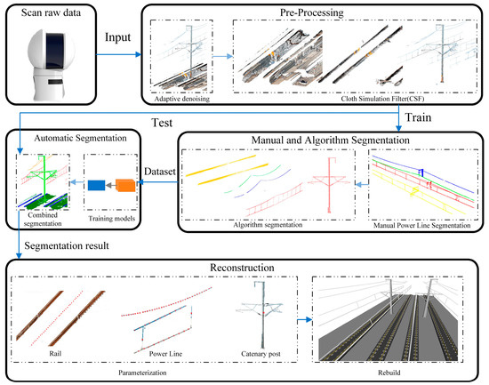
Figure 1. Flow chart of reconstruction of key railroad structure model.

3.1. Data Preprocessing

This section preprocesses the raw point cloud data to achieve adaptive denoising and scene segmentation.

3.1.1. Adaptive Denoising

As mentioned earlier, it is inevitable to have noise in point clouds, which can mainly be classified into two types: outliers that clearly deviate from the structure, and noise that appears on the surface of the structure. In addition, due to factors such as scanning equipment and methods, the final data density collected can also vary, and the density of point cloud datasets for almost any railroad scene is different.

Therefore, it is extremely difficult to use existing general solutions to achieve noise reduction for railroad scene point clouds with minimal data loss. However, compared to surface noise, outliers clearly do not fall within the model range and can have a greater impact on subsequent point cloud processing and analysis. Therefore, in denoising, the processing of such points will be given priority. Existing general algorithms require manual adjustment of various parameters and have poor adaptability. Therefore, a joint filtering method was designed in this paper to perform adaptive denoising on the data, as shown in Figure 2.

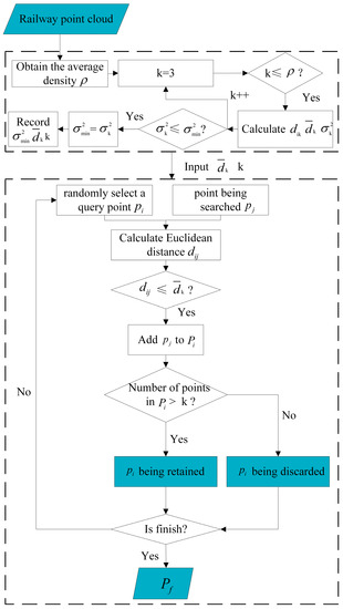
Figure 2. Flow chart of adaptive denoising.

The principle of statistical filtering (PSF) method is to calculate the average distance from each point to its specified k-nearest neighbors, and the average distance calculated for all points in the point cloud should follow a Gaussian distribution. On the other hand, the radius-based filtering method is an algorithm that has a significant filtering effect on outliers in point clouds. The two methods have their own emphasis on denoising, with the former focusing more on using neighborhood information for smoothing, and the latter focusing more on using neighborhood information to remove obvious outliers while preserving edge information. Theoretically, their combination can effectively remove a large number of outlier points, but both methods need to consider the relationship between the central point and the surrounding points. In practice, it is difficult to directly specify parameters for such algorithms based on point cloud density, and inappropriate parameters may cause significant data loss.

In this work, we use KD-Tree to search for each point as a sampling point $p_i$ and search for $k$ neighboring points. The resulting index relationship is denoted as $P_{ik}=\{p_i(x_{ij},y_{ij},z_{ij})|j=1,2,3,\dots ,k\}$. Then, we calculate the average Euclidean distance $d_{ik}$ between the sampling point and its $k$ neighboring points, the current overall average Euclidean distance ${\overline{d}}_k$, and the variance of the sampling point and the global variance ${\sigma }_k^2$, where $N$ represents the total number of points within the point cloud:

$$d_{ik}=\sqrt{\frac{{\displaystyle {\sum }_{j=1}^k{(x_{ij}-x_i)}^2+{(y_{ij}-y_i)}^2+{(z_{ij}-z_i)}^2}}{k}}$$

(1)

$${\overline{d}}_k=\frac{{\displaystyle {\sum }_{i=1}^N{d}_{ik}}}{N}$$

(2)

$${\sigma }_k^2=\frac{{{\displaystyle {\sum }_{i=1}^N(d_{ik}-{\overline{d}}_k)}}^2}{N}$$

(3)

Starting with $k$ = 3, the abovementioned calculation process is traversed and the minimum ${\sigma }_{\min }^2$ and corresponding $k$ ${\overline{d}}_k$ values are recorded, resulting in a KD-Tree clustering method that can adapt to the varying point cloud densities of different devices and better express the structural characteristics.

Using this organization method for radius filtering, the basic principle is to first randomly select a query point and set the minimum number of points M and the maximum radius $R_{\max }$. Then, search for points within the range and calculate the Euclidean distance $d_{ij}$ between the query point and the searched points, which can be represented as:

$$d_{ij}=\left|p_i{p}_j\right|=\sqrt{{(x_i-x_j)}^2+{(y_i-y_j)}^2+{(z_i-z_j)}^2}$$

(4)

where $p_i$ and $p_j$ are the query point and the point being searched, respectively, and $x_i$,$y_i$,$z_i$ correspond to the coordinates of the point cloud.

Here, we set the minimum number of points M to be the k value, and the maximum radius $R_{\max }$ to be ${\overline{d}}_k$. After traversing the range of ${\overline{d}}_k$ around the query point $p_i$ and searching for points within this range, if the number of points in the point cloud $P_i$ is greater than $k$, then the query point $p_i$ is retained in the point cloud, as shown in Figure 3.

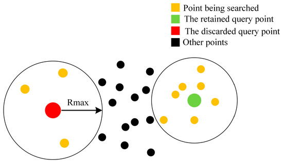
Figure 3. Schematic illustration of denoising by radius filtering.

After the adaptive filtering process, the resulting filtered point cloud is named $P_f$. This process is capable of adapting to the different density characteristics of point clouds and can quickly and simply remove obvious outlier points while preserving the boundaries of the point cloud.

3.1.2. Scene Segmentation

The railroad environment can be considered as a scene with significant differences between the ground and overhead line structures. To achieve segmentation of these structures, it is necessary to separately consider the two scenes. However, the large amount of railroad data implies a tremendous manual effort in scene partitioning. Moreover, within the ground scene, there exists the challenge of separating the actual ground from the railroad tracks. In complex ground conditions, the height difference between them becomes ambiguous, making segmentation extremely difficult without intensity information.

To address these issues, we introduce an improved approach based on the CSF method, adapted for railroad environments, to achieve automated partitioning of the ground and overhead line scenes. This enables automatic separation of the actual ground from the railroad tracks in complex ground scenes.

(1)

Related Concepts on CSF.

CSF employs a completely different approach from traditional filtering algorithms that consider slope and elevation changes to distinguish “ground points” and “non-ground points”. As shown in Figure 4, the algorithm first flips the point cloud model upside down and assumes a piece of cloth under the influence of gravity is draped over the model, with the boundary of the point cloud that comes into contact with the cloth representing the “current terrain”. Due to space constraints, this paper mainly introduces the relevant principles of railroad scene segmentation and the specific algorithm is not discussed further.

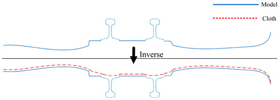
Figure 4. CSF concept.

This method treats the model as a grid composed of particles with mass and interconnecting springs. The displacement calculation of the particles considers two aspects: the displacement of particles under gravity force and the displacement of particles under internal force, where the latter connects the particles through springs. Therefore, the algorithm adjusts the particle displacement by traversing each spring, and it uses a 1-D method to compare the height differences between the two particles that make up the current spring, attempting to move particles with different heights to the same level.

Since particles can only move in the vertical direction, their movability can be determined by comparing their height with that of the ground. If a particle’s height is lower than or equal to the ground height, it is designated as immovable. If both points in the spring can move, they will be moved in opposite directions based on the average distance between them. If one point cannot move, the other will be moved. If the two points have the same height, they will not move. Thus, the displacement of each particle can be calculated by the following formula:

$$\overrightarrow{d}=\frac{1}{2}b(\overrightarrow{p_i}-\overrightarrow{p_0})•\overrightarrow{n}$$

(5)

where $\overrightarrow{d}$ represents the adjustment displacement vector, $b$ represents the particle movement determination, which is 1 if movable and 0 otherwise, $\overrightarrow{p_i}$ and $\overrightarrow{p_0}$ represent the coordinate vectors of the particle and the connected particle, respectively, and $\overrightarrow{n}=(0,0,1)$ represents the normal vector in the vertical direction.

Iterate this process with Rigidness representing the number of iterations. The distance moved each time is half of the previous one, as shown in Figure 5a. Typically, Rigidness is set to 1, 2, and 3, and the greater the number of iterations, the greater the stiffness of the cloth.

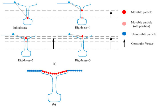
Figure 5. Principle of applying the CSF method to rail segmentation. (a) Parameterization of rigidness. (b) Iterative effect.

In principle, due to the relative continuity of the ground in the railroad environment, there will be obvious gaps in the point cloud at the bottom of the rail, as shown in Figure 4. Considering the displacement module under internal force can prevent particles from falling into the rail area, the ground and non-ground areas can be segmented even if the ground is uneven. Therefore, this method can achieve scene pre-segmentation in the absence of information such as height thresholds, and the effect is shown in Figure 5b.

(2)

CSF Adaptive Method for Rail Structure Extraction

In [54], the algorithm mentions three adjustable parameters related to the purpose of this paper: grid resolution (GR), Rigidness, and time step length (dT). The effect of the Rigidness has been detailed above and set to 3. dT determines the gravitational displacement of particles, and its value should be slightly less than H/Rigidness (where H is the height of the rail), to avoid misjudgment of some rail structures.

GR represents the horizontal distance between two adjacent cloth particles and is a crucial parameter for obtaining surface features of the railroad structure. However, setting this parameter manually can result in either large distances between cloth particles, causing difficulty in fitting the ground and leading to misidentification of rails as ground, or small distances, causing excessive computational burden. Adjusting this parameter poses a significant challenge for industry practitioners.

Moreover, the original method did not take into account the potential impact of noise on the positioning determination of cloth particles, resulting in unsatisfactory results when dealing with tasks that require high segmentation details. Considering the adaptive denoising process mentioned above, this paper introduces a pre-judgment step prior to the algorithm to address this issue, setting the GR as $r_{\max }$ adaptively obtained during the denoising process. Then, the point closest to the center within the grid and able to form K neighboring points within the grid is selected as the position of the cloth particle in the grid. If the number of points in the grid is insufficient, no particle placement is set to avoid the impact of remaining noise on the computation. Otherwise, an erroneous distribution, as shown in Figure 6b, would be generated. In practice, discarding some positioned cloth particles due to internal forces does not lead to significant errors in ground detection. Following the particle placement principles illustrated in Figure 6a, a distribution pattern like Figure 6c is formed.

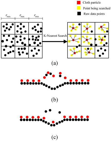
Figure 6. Cloth particles selection and distribution (a) Selection principle, (b) Original distribution, (c) Adjusted distribution.

The aforementioned approach involves placing cloth particles in relatively dense regions to avoid the influence of noise, resulting in a more accurate fitting of the particles to the ground and a more detailed representation of surface variations. Additionally, when dealing with railroad scenes, leveraging the structural characteristics of the rail tracks and the ground enables a more convenient segmentation process. Industry practitioners can simply set the rail height based on different rail types to configure the parameters, greatly reducing the complexity of use and enabling adaptation to railroad environments. The detailed algorithmic workflow of the CSF method will not be further elaborated here.

(3)

Railroad Scene Segmentation Scheme

Processing of point cloud data $P_f$ was performed according to the workflow shown in Figure 7. Firstly, the native CSF algorithm was directly applied to $P_f$ the point cloud to achieve segmentation of ground with rails and overhead lines. Then, the ground data with rails is segmented again using the proposed method in this paper, and the resulting segmented regions of overhead lines, ground, and rails were labeled as $P_{f-OL}$, $P_{f-ground}$, $P_{f-rail}$, respectively, for ease of identification of the processing steps and point cloud scenes.

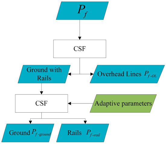
Figure 7. Railroad point cloud processing process based on CSF.

Due to the relatively high Rigidness, the segmented rails may contain irrelevant points caused by protruding areas of the original ground. Therefore, further refinement of the rails area is necessary.

3.2. Rail Segmentation

$P_{f-rail}$ have been extracted previously, and in this section, the rail structure is segmented based on factors such as the rail structure and size. Due to various reasons, there may be certain differences between point cloud data of rails at different locations, making it difficult to segment them using a holistic method. In this paper, the model is sliced in the forward direction and processed in segments, with each segment slice represented as $C_i$, as follows:

First, the algorithm selects either side of the rail cross-section $C_i$ for analysis, and then, in descending order of elevation values, a certain number of points are chosen (three points are shown in the figure for illustrative purposes, typically 10 or more points can be selected). Then, the algorithm calculates the curvature at each of these points by estimating the normal vectors with respect to the adjacent points within the same cross-section, as illustrated in Figure 8a–c.

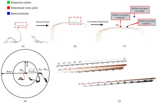
Figure 8. Segmentation of rail points. (a) Origin point data, (b) possible vertex points, (c) curvature calculation result, (d) obtaining the vertex from another rail, and (e) extracted results.

Subsequently, the algorithm identifies the highest point with relatively stable curvature as the vertex $p_{h1}$, denoted by the red point in Figure 8c.

Next, as depicted in Figure 8d, the algorithm draws a circle based on the track gauge information. It then repeats the same process as in Step 1 for the other side of the rail section, within the coordinate range defined by $R_{\max }$ and $R_{\min }$ (the specific values of $R_{\max }$ and $R_{\min }$ depends on the track gauge). The algorithm determines a set of candidate points $p_{h0}$ and calculates the vector $\overrightarrow{p_{h0}{p}_{h1}}$ between $p_{h0}$ and $p_{h1}$. The algorithm then evaluates the angles between this vector and the ground for each $p_{h0}$ and selects the candidate point with the smallest angle as the other vertex $p_{h2}$.

After the $p_{h1}$ and $p_{h2}$ are determined, the range of the planes of the two rails is determined based on the size information, and all points below the plane are taken as rail points in $C_i$. Finally, the entire process is iterated for all slices, as shown in Figure 8e, to achieve rail segmentation for the entire section and obtain the final rail point cloud $P_{f-rail}$.

3.3. Power Line and Catenary Post Segmentation

This section focuses on the segmentation of three types of structures in $P_{f-OL}$: messenger-wire, double-chain suspension line, and catenary post. The term “double-chain suspension lines” here refers to power lines that include conductors, messengers, and suspension cables. Power lines are prone to low data density or discontinuities during the scanning process, and there may be poor segmentation results at the connection between power lines and catenary posts. In order to optimize the segmentation of power lines and catenary posts, this paper improves the existing commonly used mixed model fitting method (including PCA and RANSAC algorithm) [61,68] by integrating columnar search method, to achieve accurate segmentation and noise reduction of power lines, and to extract catenary posts by taking the difference set. The overall process can be summarized in Figure 9. To facilitate the intuitive display of the effect, this section will use a power line in contact with a catenary post as a data example.

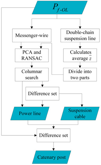
Figure 9. Process flowchart for an overhead line.

3.3.1. Candidate Points for Power Line Rough Extraction

Although power lines are distributed in three-dimensional space, they typically exhibit good linear characteristics when projected onto the XY plane. Taking advantage of this feature, the PCA algorithm is used for the coarse extraction of power line candidates. As this algorithm is widely applied, the detailed process is not elaborated here.

The core parameter of this algorithm is the use of the linear measure $\alpha ={\lambda }_1/{\displaystyle {\sum }_{i=1}^3{\lambda }_i}$ [69] for classification. Here, $\lambda$ refers to the eigenvalues extracted from the covariance matrix decomposition of the local plane established during the PCA calculation. The detailed calculation process is not described here. If α is greater than the set threshold, it is classified as a candidate point. When dealing with curved line segments, this value can be appropriately relaxed. For the example data processing, the extracted candidate points are shown in Figure 10a.

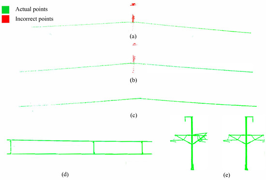
Figure 10. Segmentation of the line. (a) The result of the PCA method processing, (b) the result of the processing after adding RANSAC, (c) the result of the processing after adding columnar search, (d) the result of the extraction of the double chain suspension line, and (e) the result of the extraction of catenary post.

The RANSAC algorithm can accurately fit the parameterized equation of a model and achieve some level of denoising when dealing with data containing irrelevant structures [70]. The key parameter is the allowable distance D between points and the parameterized equation, which is usually considered as 0.1 m, meeting the requirement for extracting power lines. The optimization result is shown in Figure 10b. However, this method still filters points from a two-dimensional perspective, making it difficult to completely remove irrelevant points in space while preserving the integrity of power lines.

3.3.2. Precise Extraction Method Based on Columnar Search

Due to the linear geometric structure of power lines in space, this paper proposes a columnar search method to achieve precise extraction. The process is shown in Figure 11.

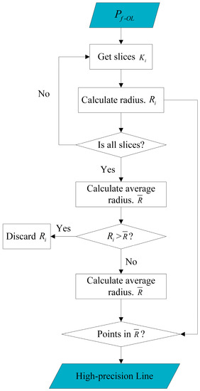
Figure 11. Flowchart of the columnar search.

Using the same slicing method as in Section 3.2 for rail segmentation, each segment is defined as $K_i$, and the radius $R_i$ of $K_i$ is obtained by calculating the average height difference between all points in $K_i$ and the centroid.

$$R_i=\frac{1}{n}{\displaystyle {\sum }_{j=1}^n\left|z_j-\overline{z}\right|}$$

(6)

where $R_i$ and $n$ represent the fitting radius and number of points in the $K_i$ slice, and $z_i$ and $\overline{z}$ represent the z coordinate of the point $j$ in the slice and the average z coordinate of all points, respectively.

Next, based on all the $R_i$, the average value $\overline{R}$ of the entire segment is calculated, and any $R_i$ greater than $\overline{R}$ is removed. Then, a second average value $\overline{R}$ is calculated as the final value. Afterward, only the points within distance $\overline{R}$ from the centroid are retained in each slice $K_i$, thus achieving the extraction of a relatively complete, low noise and intact power line point cloud with intact junctions, as shown in Figure 10c.

3.3.3. Precise Extraction Method for Composite Model of Double-Chain Suspension Line

First, the same slicing method is used to obtain the slice $K_i$, and then the average height $\overline{z}$ of the points in $K_i$ is calculated. Based on this value, the model is divided into upper and lower parts, and the processing flow of Section 3.3.2 is performed on each part to extract the conductor and messenger wire parts of the model. Then, the middle line between the two wire parts in $K_i$ is extracted to obtain the suspension cable part of the model. The process is illustrated in Figure 12, and the overall extraction effect is shown in Figure 10d.

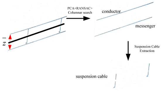
Figure 12. Extraction process of the double-chain suspension line.

Finally, for the two types of power lines extracted from $P_{f-OL}$, the complete catenary post model can be obtained by taking the difference set and performing minimum clustering. The extraction results are shown in Figure 10e.

3.4. Performance Validation

The advantages of the proposed segmentation algorithm in this paper are mainly reflected in two aspects: the segmentation of ground and steel rails in complex railroad environments without relying on the intensity information and line direction information, and the preservation of the completeness of power lines. Therefore, two scenes were tested, which contain different railroad data and most importantly, completely different ground styles for comparison. The power lines also have a lot of interference, including the problem of contact between lines and supports, as well as noise. Additionally, these data come from different scanning methods, different regions, different point cloud densities, and different structural compositions, which can provide a test for the algorithm’s adaptability. Finally, CloudCompare software [71] was used to display the point cloud, and all other algorithms were implemented by programming. The input data here are a set of point clouds $P=\{p_1,p_2,p_3\dots p_n\}$ containing Euclidean coordinates and RGB color information, and any point can be described as $p_i=(x_i,y_i,z_i,r_i,g_i,b_i),1\le i\le n$.

3.4.1. Case of Study

The first scene (referred to as Scene A), was obtained by scanning with a LiGrip H120 handheld laser scanner at the site, as shown in Figure 13a,b. The device has a maximum measurement range of 120 m, a scan field of view of 280° × 360°, and a scanning frequency of 320,000 pts/s. The scanning trajectory of the device is shown in Figure 13a, and the scanning process is shown in Figure 13c. The resulting scene shown in Figure 14a consists of approximately 2 km of ballasted railroad. To facilitate the validation of the segmentation algorithm in this section, it was divided into a point cloud of approximately 450 m in length, which is the same length as the second scene, and the remaining point cloud was used for deep learning validation in the next section. During the scanning process, the track was undergoing major repairs, and the ground was extremely uneven, with no fixed pattern of protrusions or depressions. Some parts of the ground even rose higher than the track. Furthermore, due to the handheld scanning, the trajectory information collected by the device had no practical value and required significant adjustment for segmentation work. The specific information on the total number of points, density, and accuracy of the scene is shown in Table 1, where the accuracy is derived from the scanning device.

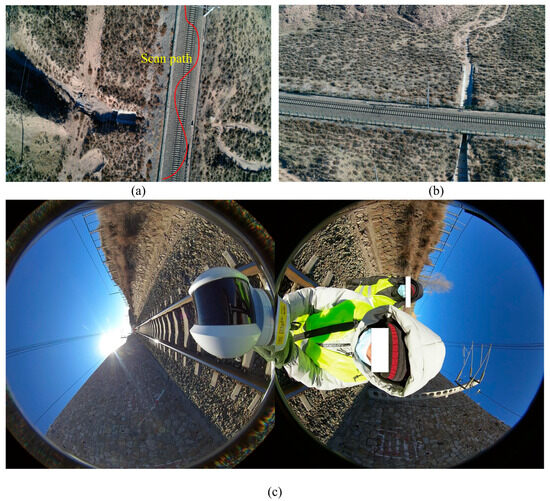
Figure 13. Data sources for Scene A: (a,b) railroad track; (c) scanning equipment.

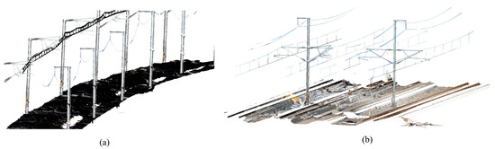
Figure 14. Railroad scenes: (a) self-test railroad dataset; (b) WHU-TLS railroad dataset.

Table 1. Case studies’ data.

Scene	Length (m)	Total Points (Million)	Point Density $(\mathbf{Points}/{\mathbf{m}}^2$)	Range Precision
A	2000	137.28	297.54	±3 cm
B	450	29.73	3366	—

The second scene (referred to as Scene B), was obtained from the publicly available WHU-TLS dataset [72] Railroad module. This scene contains four ballastless tracks, as well as rail and ground data, with an effective length of approximately 450 m, as shown in Figure 14b. The ground data in this scene is relatively flat, making the segmentation of ground and steel rail easier and more suitable for comparison with the first scene. However, this scene has multiple tracks and a complex distribution of power lines, which presents some challenges for the automation of segmentation algorithms. The total number of points and density information for this scene is presented in Table 1, while the accuracy information is not publicly available.

3.4.2. Evaluation Method

To compare with the proposed improved CSF method in this paper, we also processed the data using the PMF method, with its parameters including the local minimum surface resolution (Rs), the maximum expected slope of the ground (MaxS), the maximum window radius (MaxW), the elevation threshold for point classification (Et), and the elevation scaling factor for the scaled elevation threshold (Es). The optimal values of these key parameters were selected as the experimental basis [51], and the data was processed following the railroad scene segmentation scheme proposed in this paper.

The subsequent steel rail segmentation and power line segmentation are for further optimization or fine segmentation of the divided scenes, and the experimental data under the optimization method proposed in this paper is directly presented for performance evaluation.

Meanwhile, in order to evaluate the effectiveness and efficiency of each method, we introduce the concept of Intersection over Union (IoU). It considers the model-predicted segmentation result as one set and the true segmentation result as another set and calculates the intersection and union of the two sets to obtain a value, which measures the degree of overlap between the model-predicted segmentation result and the true segmentation result and can express the segmentation accuracy. The formula can be written as

$$IoU=\frac{TP}{TP+FP+FN}$$

(7)

where $TP$, $FP$, and $FN$ represent true positive, false positive, and false negative, respectively.

3.4.3. Results and Analysis

After being processed by the adaptive denoising algorithm, for quantitative demonstration of the denoising effect, we conducted further manual processing based on the results obtained from a specific scene. The specific details of the adaptive algorithm and the denoising results are shown in Table 2 and Figure 15, respectively.

Table 2. Adaptive denoising data.

Scene	${\overline{\mathit{d}}}_{\mathit{k}}$	${\mathit{\sigma }}_{\mathbf{min}}^2$	K	Detail Scene	Outlier Points Recognized by Manual Operation	Outlier Points Recognized by Algorithm	Denoising Rate (%)
A	0.1295	0.0137	141	Ground	371,955	347,034	93.3
				Over Line	16,609	14,881	89.6
B	0.1273	0.0499	17	Ground	734,654	702,329	95.6
				Over Line	65,413	60,899	93.1

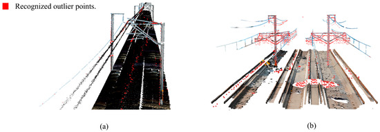
Figure 15. Adaptive denoising effect: (a) Scene A; (b) Scene B.

In Scene A, the noise points primarily originate from the walking trajectory of the operators using handheld scanning devices and surface noise from certain overhead line structures. In Scene B, the noise mainly comes from surface point drift and void areas of the overhead line structures, resulting in a higher number of noise points and longer offset distances. However, overall, the evident noise points in both scenes have been removed, indicating that the proposed adaptive denoising method can adaptively establish a KD-Tree based on different input datasets, overcoming the characteristics and types of various data. It achieves high-precision outlier denoising for the overall structure without significantly losing overhead line data. This allows practitioners to avoid the tuning problems associated with traditional filtering algorithms, thereby greatly enhancing the efficiency of the denoising work.

According to the scene division scheme proposed in this paper, two denoised scenes were processed. The first CSF processing was implemented using default parameters, while the grid resolution GR for the second CSF processing was determined based on the ${\overline{d}}_k$ value of the scene. The Rigidness was set to 3, and the rail height H was set to 176 mm according to the actual scanned rail height. The time step dT was set to 58 mm. The segmentation parameters and results are shown in Table 3. Combined with Figure 16 and Figure 17, and the data, it can be seen that for flat ground like scene B, both CSF and PMF algorithms can segment the required scene. However, for the curved track and uneven ground of scene A, the PMF method cannot segment the rail area.

Table 3. Segmentation data results.

Methods	Parameters	Stage 1	Stage 2	Scene	Classification	IoU	Runtime (s)
CSF	GR	2	${\overline{d}}_k$	A	Overhead lines	0.9699	2.1
	Rigidness	1	3		Rails	0.5258
	H (m)	1	0.176	B	Overhead lines	0.9736	1.6
	dT (m)	1	0.058		Rails	0.7004
PMF	Rs (m)	1.5	1.5	A	Overhead lines	0.9616	79,089.7
	MaxS	0.2	0.1		Rails	—
	MaxW (m)	5	5	B	Overhead lines	0.9845	106,522.3
	Et (m)	0.4	0.4		Rails	0.7032
	Es	0.4	0.1

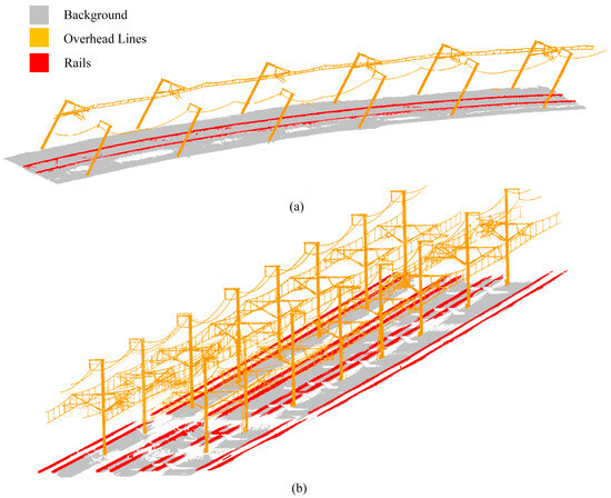
Figure 16. Scene segmentation results based on CSF: (a) Scene A, (b) Scene B.

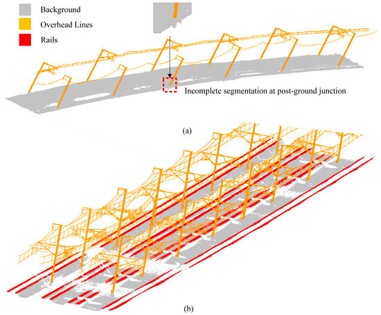
Figure 17. Scene segmentation results based on PMF: (a) Scene A, (b) Scene B.

In terms of performance, using the CSF method proposed in this paper to process two scenes of approximately 450 m each took about 2 s, while the processing time using the PMF method may even be higher than manual processing. In terms of accuracy, the two methods have relatively close IoU values in the segmented areas, with a minimum of 0.9616 for the overhead line area. However, the PMF method based on the height difference information may result in incomplete segmentation at the junction between the post and the ground, as shown in the enlarged area in Figure 17a. The IoU of the rail area is as low as 0.5258, mainly because the segmented area is larger than the actual area, but it can be seen from the results that the rail area can be fully preserved for subsequent fine segmentation processing.

Prior to this, due to the possibility of different numbers of tracks and distances between them in different scenes, we did not set up adaptive processing for multiple railroad tracks. Therefore, we manually segmented each track in scene B and processed them separately for subsequent analysis.

It can be seen that in the case of complex railroad scenes, relying solely on elevation information for segmentation is difficult to implement. However, with the CSF processing scheme proposed in this paper, adaptive segmentation of complex railroad scenes can be achieved with only the steel rail height parameter H set for the track used. Subsequently, the steel rail areas of the two scenes were subjected to the steel rail fine segmentation proposed in Section 3.2 of this paper, and the changes in the areas are shown in Figure 18, with the corresponding IoU changes listed in Table 4.

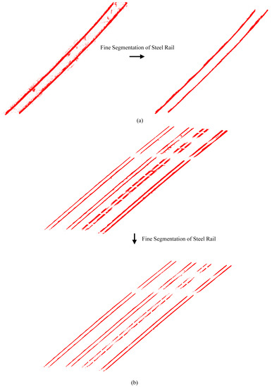
Figure 18. Rail segmentation results: (a) Scene A, (b) Scene B.

Table 4. Rail segmentation data results.

Scene	Runtime (s)	IoU Previous	IoU after
A	15.4	0.5258	0.8814
B	71.9	0.7004	0.9613

The results demonstrate that this study integrates the development of an adaptive filtering algorithm and an improved CSF method for data preprocessing. Subsequently, a novel rail segmentation approach is employed for fine-tuning. Compared to mainstream rail segmentation methods [22,28,48], our proposed method achieves precise rail point segmentation solely based on point cloud coordinate data without relying on track alignment or intensity information. Furthermore, the proposed method fulfills the required accuracy and efficiency demands for data processing, significantly reducing the challenges and costs associated with obtaining authentic rail point cloud data in the field of railroad engineering maintenance and operation.

In the process of extracting power lines, due to the different distribution and quantity of power lines in the two scenes, we manually pre-divided each power line area so that each point cloud contains only one power line, including surface noise points and catenary posts. Because the structure is located in the air and is far apart, this process is easy to implement.

For the segmentation of power lines and catenary posts in the overhead wire area of the two scenes, the effectiveness of each process in the segmentation method has been described in detail in Section 3.3, and the processing results are shown directly in Figure 19. In terms of parameter settings, the key parameters of the PCA and RANSAC algorithms are relatively conservative. The linear metric $\alpha$ is set to 0.6 and the allowable distance D is set to 0.1. The subsequent columnar search approach requires no parameter settings, enabling adaptive detection of the direction of power lines, whether they are straight or curved, and precise segmentation of messenger-wire and double-chain suspension lines.

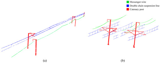
Figure 19. Overhead lines segmentation results: (a) Scene A, (b) Scene B.

In summary, by combining commonly used hybrid segmentation methods [59] with the proposed Columnar search method, the IoU for power line segmentation has been significantly enhanced without incurring noticeable time overhead. Compared to previous efforts that extracted power lines from overhead line data [61] with an IoU of 0.9360, the results obtained in this study achieved an impressive IoU of 0.9981, as detailed in Table 5. This substantial improvement allows for more precise extraction of power line data from point cloud datasets, thereby providing accurate information for automated modeling and other related tasks.

Table 5. Power line segmentation data.

Methods	Parameter	Runtime (s)	IoU
PCA	$\alpha$ 0.6	26.6	0.9283
+RANSAC	D 0.1	+6.0	0.9302
+Columnar search		+6.6	0.9981

4. Automatic Segmentation Verification

As mentioned in the earlier validation process, railroad scenes may involve a complex spatial distribution of multiple tracks and power lines, which do not have fixed distribution rules and require manual adjustments for algorithmic segmentation. To address this, this paper introduced a deep learning method for automation, replacing the parts that still require manual processing (such as scene segmentation for multiple track and power line scenes) with a deep learning segmentation approach, and combining it with segmentation algorithms to achieve efficient and accurate point cloud data segmentation.

4.1. Data Description

The semantic segmentation data obtained from the performance verification in Section 3 were used as the dataset for evaluation. The dataset consists of five different types of structures, and the results are shown in Table 6.

Table 6. Distribution of classes.

Scene	Total Points	Background	Rails	Catenary Post	Messenger-Wire	Double Chain Suspension Line
Scene A	29,638,949	26,605,500	1,838,351	471,642	165,151	558,305
Scene B	29,009,362	22,731,479	3,791,550	1,834,265	156,682	495,386

4.2. Deep Learning

4.2.1. Parameter Configuration

In Section 2, it was mentioned that the RandLa-Net network improved the random sampling and aggregation of local features for 3D point clouds in large scenes, making it suitable for training point cloud segmentation in railroad environments. Therefore, this paper utilized this deep learning network for training and constructed the environment based on the Tensorflow machine learning and artificial intelligence framework. The training hardware configuration is as follows: GPU: NVIDIA GeForce RTX 3070, CPU: AMD Ryzen9 5900X, RAM: 32 GB DDR4.

4.2.2. Training Data Preprocessing

Point cloud data in different formats may have varying attribute descriptions. This paper took into account the features of the RandLa-Net network and dataset and used only the Euclidean coordinates and RGB information of each point cloud as input. This can be represented as follows:

$$X_{N\mathrm{x}6}=\left[\begin{array}{ccc}\begin{array}{ccc}\begin{array}{c}{x}_1\\ ⋮\\ x_N\end{array}& \begin{array}{c}{y}_1\\ ⋮\\ y_N\end{array}& \begin{array}{c}{z}_1\\ ⋮\\ z_N\end{array}\end{array}& \begin{array}{c}{r}_1\\ ⋮\\ r_N\end{array}& \begin{array}{cc}\begin{array}{c}{g}_1\\ ⋮\\ g_N\end{array}& \begin{array}{c}{b}_1\\ ⋮\\ b_N\end{array}\end{array}\end{array}\right]$$

(8)

where $N$ represents the number of point clouds, $(x,y,z)$ represents the Euclidean coordinates of a point, and $(r,g,b)$ represents the color information of a point.

(1)

Down-sampling

The original point cloud data collected by the device are often very large. To input the data into the network, a downsampling process that does not affect the geometric features is performed to reduce the data size. First, the original data and the point clouds downsampled in the grid format (using a grid width of 0.8 m for this dataset) are both saved in the ply format, and a kdtree file is created for the downsampled points to retain the corresponding relationship with the original data, facilitating quick input of the point cloud into the network. Secondly, the nearest downsampled point is assigned to each point in the original data, and a proj file is created to save the corresponding relationship, making it easier to obtain labels for the original data from the downsampled point cloud after semantic segmentation.

(2)

Training data generator

To obtain the local features of the entire point cloud, a random and comprehensive selection of local point clouds is necessary, from which data and labels are extracted for input into the network. The generator first assigns a random probability value to each point and selects the point with the minimum value as the center point. Then, a batch of points near the center point is obtained based on the preset number of points fed in at a time and the kdtree file. Next, the probabilities are updated considering the distance between this batch of points and the center point, as well as the weight of the number of points in each category (i.e., the proportion of this category in the dataset). This ensures that all parts of the point cloud can be adequately represented. Finally, the necessary training data and corresponding labels are extracted from this batch of points to generate a unit of training data. This process is iterated for the entire point cloud to generate the global training data.

(3)

Data augmentation

To enhance the model’s applicability, it is often necessary to expand the dataset through data augmentation, which enables the model to better generalize to new data. After generating the training data, this batch of data can be transformed through rotation, scaling, translation, and other techniques to create more diverse data samples. This process enables the model to better handle different inputs and improve its overall performance.

For verification and testing, this paper divided the training and validation sets according to the method shown in Table 7, where “m” represents meters of track-length.

Table 7. Distributions of training/test sets.

Scene	Training Set (m/%)	Test Set (m/%)
Scene A	450/22	1550/78
Scene B	90/20	360/80

4.2.3. Training Evaluation Parameters

Training was performed with an initial learning rate of 0.01, a learning rate decay rate of 0.95, a total of 100 epochs, 500 training steps per Epoch, 100 validation steps, a batch size of 4, and 500 points input per step.

To evaluate the model’s performance, this paper recorded the $Accuracy$ and $Loss$ data during the training process and recorded the $IoU$ for each class and the overall $mIoU$ during the testing process. The definitions of these indicators are as follows:

$$Accuracy=\frac{TP+TN}{TP+TN+FP+FN}$$

(9)

where $TN$ represents true negative, and $Accuracy$ represents the proportion of correctly predicted samples to the total number of samples.

$$Loss={\displaystyle {\sum }_{i=1}^C{w}_i\times (-y_i\times \log p_i-(1-y_i)\times \log (1-p_i))}$$

(10)

where $C$ represents the number of classes. $y_i$ represents the probability distribution of the true class, $p_i$ represents the probability distribution of the predicted class, and $w_i$ represents the weight of each class.

This loss function calculates the cross-entropy between the true class $y_i$ and the predicted class $p_i$ for each class and then multiplies it by the weight $w_i$ to obtain the weighted cross-entropy. Finally, the sum of the weighted cross-entropy of all classes is obtained as the value of the total $Loss$.

$$mIoU=\frac{{\displaystyle {\sum }_{i=1}^{C}Io{U}_i}}{C}$$

(11)

$mIoU$ is the average of the $IoU$ values for all categories, used to measure the overall performance of the model, and the maximum value of this value is usually taken as the best model.

4.2.4. Training and Segmentation

To verify the effectiveness of the proposed automatic segmentation method, this paper compared two different approaches during the training process.

Approach 1 involves training the network using all five types of data in the dataset, and then performing segmentation validation directly on the complete point cloud after adaptive denoising, as shown in Figure 20a.

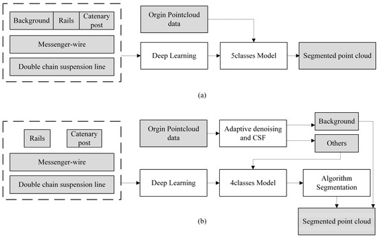
Figure 20. Flowchart for point cloud segmentation using deep learning: (a) Approach 1, (b) Approach 2.

In Approach 2, all four types of data (excluding background) are used to train the network. For segmentation validation, the complete point cloud is first separated into ground and non-ground points using adaptive denoising and CSF algorithms. The remaining points are then inputted into the trained model for scene segmentation and classification. Finally, the data is sent to the corresponding segmentation algorithm for further refinement, as shown in Figure 20b. The algorithms mentioned here are consistent with the methods introduced in Section 3.

4.3. Conclusions and Analysis

For Approach 1, the training $Accuracy$ and $Loss$ data, as well as the $mIoU$ and $IoU$ data for each class, after 100 epochs of training, are shown in Figure 21. The best $mIoU$ achieved was 0.8303, and the $IoU$ for each category is presented in Table 8. The segmentation results are shown in Figure 22a and Figure 23a.

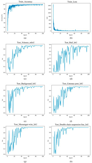
Figure 21. Training results for Approach 1.

Table 8. Results of segmentation.

Scene	Ground Data	Train Runtimes (min)	mIoU	Rails	Background	Catenary Post	Messenger-Wire	Double Chain Suspension Line
Scene A	No	51	0.9518	0.9999	—	0.9359	0.9245	0.9471
	Yes	87	0.8265	0.5117	0.8471	0.9369	0.9318	0.9052
Scene B	No	59	0.9665	0.9999	—	0.9029	0.9900	0.9734
	Yes	113	0.8303	0.7596	0.9333	0.8183	0.9943	0.9852

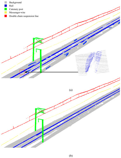
Figure 22. Automatic segmentation results for scene A: (a) Approach 1, (b) Approach 2.

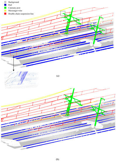
Figure 23. Automatic segmentation results for scene B: (a) Approach 1, (b) Approach 2.

For Approach 2, the training $Accuracy$ and $Loss$ data, as well as the $mIoU$ and $IoU$ data for each class, after 100 epochs of training, are shown in Figure 24. Compared with direct segmentation, all data improved significantly. The best $mIoU$ achieved was 0.9665, and the $IoU$ for each category is presented in Table 8. The specific segmentation results are shown in Figure 22b and Figure 23b.

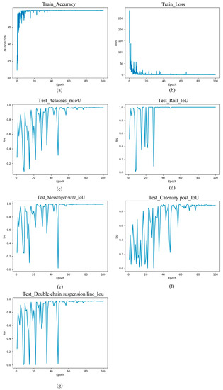
Figure 24. Training results for Approach 2.

Based on the results, it is evident that Approach 1, as a comparative method, was prone to significant segmentation errors due to unclear boundary features between the rail and the ground. This leads to frequent missing parts of the rail and poor segmentation performance in the zoom-in area where the power line and catenary post intersect, as illustrated in Figure 23. The overall $IoU$ of each structure is also lower, making it challenging to ensure the accuracy of segmentation results for modeling or other purposes, and thus, it is not suitable for production use.

On the other hand, Approach 2, with the proposed processing pipeline, achieved a higher $IoU$ of above 0.9 for each structure while maintaining a model accuracy of 1. This success indicates that automatic segmentation for each structure in both scenes is achieved, with a processing time of less than 1 min per kilometer for the single-track line scene A.

Existing semantic segmentation approaches for complex railroad point clouds [67] have explored various deep-learning network segmentation techniques, achieving an overall best $mIoU$ of 0.9095. The best $IoU$ for rails reached 0.8376, and for cables, it reached 0.9239. However, the $IoU$ for most structures fluctuated between 0.5 and 0.8, with a minimum training time of 113 min. Additionally, significant discrepancies in test results were observed among different datasets. The study concluded that the current deep-learning methods struggle to address noise interference. It was evident from the discussion and results that processing large-scale point cloud data directly using pure deep learning networks results in long training times, difficulty in identifying noise interference, and errors in segmenting local rail and Catenary posts from the ground, similar to Approach 1 used in this paper. Moreover, the segmentation performance was poor for special railroad structures such as informative signs and traffic signs. Furthermore, due to the variability of railroad scenes, the model’s generalization capability when applied to other datasets was limited, restricting its applicability in specific engineering projects.

As a point of comparison, this study introduced a novel workflow that begins with the application of an adaptive denoising method for noise reduction. Subsequently, deep learning techniques were employed to handle the pre-classification and segmentation of extensive point cloud data, followed by the integration of corresponding segmentation algorithms to extract key structures. The efficacy of these algorithms was validated in earlier sections, demonstrating stable performance across different datasets. The proposed approach achieved $IoU$ of 0.9 and above for the key structures of interest, even as the number of points increases, with a notable reduction in training time. Researchers can utilize our segmentation algorithm to create localized datasets specific to railroad lines, enabling automated segmentation for most structures with similar characteristics. Consequently, this enhances the method’s applicability to specific railroad engineering projects and offers valuable insights for achieving efficient and accurate automation of critical structure segmentation directly from raw point cloud data.

4.4. Model Reconstruction

The numerous point cloud data are of little significance for establishing BIM models in railroad scenes. For linear structures (including rails and power lines), the key point of modeling is to extract their directions, while for catenary supports, the key point of modeling is to extract their placement coordinates [73]. These parameterization schemes have been widely used. Therefore, this section briefly introduces the modeling methods of various structures in the scenes involved in this paper.

Parameterization and Modeling of Key Structures

Railroad structure: The centerline information of the steel rail is extracted using the least-squares method, and the railroad structure section is established based on standard design parameters. The rail model is built by integrating these two types of information, as shown in Figure 25a.

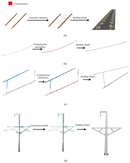
Figure 25. Process of parameterization and modeling of key structures: (a) rail structure, (b) messenger wire structure, (c) double-chain suspension line structure, and (d) catenary post structure.

Power line structure: Two types of power line structures are involved in this paper. For a messenger wire, the line shape is directly fitted. For a double-chain suspension line, the upper and lower lines are constructed in the same way as the former, and the suspension cable’s centroid coordinates are extracted, considering it as a vertical line intersecting with the upper and lower lines, as shown in Figure 25b,c.

Catenary post structure: A BIM model of the catenary post is preset, and the model is established based on its centroid coordinates, as shown in Figure 25d.

Upon completion of the three major structural models, the core model of the railroad has been successfully established. To enhance the final presentation of the BIM model, this paper further improves the overall BIM model by incorporating manually prefabricated BIM models for bridge piers, guardrails, and fasteners, along with embankment cross-sections and corresponding material textures. The entire BIM model is programmatically created using Dynamo software, as illustrated in Figure 26.

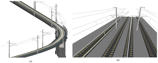
Figure 26. Modeling overall effect: (a) Scene A, (b) Scene B.

Notably, in Scene A, the placement of bridge piers, guardrails, and other equipment is automated by inputting the respective mileage positions during the programming process.

5. Discussion

As the data collected in this study originate from handheld laser scanning devices, which have relatively lower accuracy, the use of such BIM models for railroad engineering management tasks, such as the integration of GIS data and sensor data for visualization-based maintenance, can tolerate these errors without causing a significant impact on the work. However, this automated method has limitations in meeting the high-scale precision requirements for tasks such as measuring rail deformation, analyzing rail vibrations, and detecting changes in track gauges.

Noise information is the biggest influencing factor on point cloud segmentation. In railroad scenes, commonly used denoising methods can cause significant data loss to overhead line structures, and directly lead to information loss in sparsely populated areas. Moreover, excessive noise can also have an impact on ground detection. The adaptive denoising method proposed in this paper works best on data with relatively uniform density across structures. However, when different devices are used to collect data on different structures, differences in density can pose greater challenges for denoising. To avoid difficulties in processing field data, future research needs to consider denoising methods that are combined with field scanning processes.

Point cloud intensity is an essential piece of information, but its accuracy is difficult to ensure due to the influence of multiple factors, and there is relatively little work on intensity calibration. In the data collected in this paper, the intensity information can roughly show the rail surface, but some ground points’ intensity information falls into this range, causing the rail extraction algorithm to fail. Therefore, in the authors’ view, it is meaningful to combine intensity information for ground segmentation in the railroad environment, which is crucial for promoting segmentation work in more scenes. Subsequently, it is possible to consider reverse correction of stiffness information combined with geometric information to adjust erroneous stiffness information in ground points, achieving faster and more accurate classification. Of course, correcting this information during data acquisition is even more critical.

Deep learning is one of the key approaches in the automatic segmentation of point clouds. In terms of application, the same trained model performs well in situations where the railroad section or structure is similar. However, there are variations in railroad construction standards among different countries and types. Moreover, the limited availability of open point cloud datasets and the significant differences in data acquisition devices make it challenging to train highly generalizable large models that can be applied to specific engineering projects. The proposed approach of combining the segmentation algorithm presented in this paper with deep learning processing offers a solution. Creating a small dataset specific to a particular railroad ensures high-quality automated segmentation for the majority of that railroad. However, the creation of datasets for multi-line railroads involves some manual processing, which may result in increased time requirements when dealing with larger railroad scenes. In conclusion, in the railroad environment, it is difficult to enhance the generalization power of deep learning by expanding the dataset. Considering modifications to the deep learning network may be the key to improving model robustness.

Regarding the developed segmentation algorithm, this paper mainly focuses on extracting critical structures of the railroad line. For other accessory structures in the line, they have not been addressed. When facing structures that do not have obvious geometric features, the automatic segmentation process is often challenging. Therefore, corresponding segmentation methods should be designed for similar signal equipment, power supply equipment, and along-line stations’ data to provide data support for deep learning, or else there will be a large amount of manual segmentation work.

In general, current deep learning-based point cloud semantic segmentation solutions [67] and mainstream segmentation algorithms [22,48,74] mentioned earlier have made significant progress in point cloud processing in railroad environments. However, there still exist certain manual operations in dealing with noise, separating ground data, and handling complex situations such as multi-track steel rails and multiple power lines in railroads. Additionally, it remains challenging to perform point cloud semantic segmentation without relying on intensity information or trajectory information.

By employing the solutions proposed in this paper and subsequent improvements based on these techniques, it is possible to achieve low-cost and efficient processing of point cloud data in specific offline railroad environments, as well as automated semantic segmentation of key structures. This provides data support for the reconstruction of railroad environments. Moreover, tasks such as health monitoring or data visualization of railroad and other civil engineering structures will become more convenient and effortless, ensuring the safety of structures and the general public with greater accuracy.

6. Conclusions

In this paper, we proposed an automatic segmentation method for railroad point clouds, which utilizes a handheld laser scanner to acquire data and only processes coordinate information due to the higher cost of collecting accurate trajectory information and point cloud intensity information. In practical work, manual or semi-automatic processing of railroad point cloud data is usually required, but it is time-consuming and labor-intensive due to the large amount of data. Therefore, our work mainly realizes an automatic point cloud segmentation method, which includes four stages: point cloud adaptive denoising, scene segmentation, structure segmentation combined with deep learning, and model reconstruction. We validated the proposed process on two types of railroad point cloud data with significant ground differences, and the results showed that our process has strong applicability.

We achieved ground data processing through adaptive denoising combined with the improved CSF method and steel rail point extraction through the proposed double steel rail segmentation method that can resist certain surface noise. Additionally, we improved the completeness of power line structure segmentation without significantly increasing computation time, resulting in a 6% improvement over existing methods. Moreover, we proposed a process for automatic segmentation of critical structures by combining deep learning, achieving at least 90% IoU, which is more efficient and accurate than existing direct deep learning segmentation methods and supports model reconstruction.

In summary, our work provides a low-cost method for railroad line model reconstruction, allowing researchers to perform large-scale automated segmentation using only the three-dimensional coordinate data of railroad point clouds, which can reliably reduce the cost of railroad engineering operation and maintenance and improve the efficiency of BIM model construction.

References

- Chen, Z.; Haynes, K.E. Impact of high-speed rail on regional economic disparity in China. J. Transp. Geogr. 2017, 65, 80–91. [Google Scholar] [CrossRef]
- Qin, Y. ’No county left behind?’ The distributional impact of high-speed rail upgrades in China. J. Econ. Geogr. 2017, 17, 489–520. [Google Scholar] [CrossRef]
- Chen, Z.; Xue, J.; Rose, A.Z.; Haynes, K.E. The impact of high-speed rail investment on economic and environmental change in China: A dynamic CGE analysis. Transp. Res. Part A Policy Pract. 2016, 92, 232–245. [Google Scholar] [CrossRef]
- Zhu, S.; Cai, C. Interface damage and its effect on vibrations of slab track under temperature and vehicle dynamic loads. Int. J. Non-Linear Mech. 2014, 58, 222–232. [Google Scholar] [CrossRef]
- Zerbst, U.; Lundén, R.; Edel, K.O.; Smith, R.A. Introduction to the damage tolerance behaviour of railway rails—A review. Eng. Fract. Mech. 2009, 76, 2563–2601. [Google Scholar] [CrossRef]
- Bian, J.; Gu, Y.; Murray, M.H. A dynamic wheel-rail impact analysis of railway track under wheel flat by finite element analysis. Veh. Syst. Dyn. 2013, 51, 784–797. [Google Scholar] [CrossRef]
- Yin, J.; Tang, T.; Yang, L.; Xun, J.; Huang, Y.; Gao, Z. Research and development of automatic train operation for railway transportation systems: A survey. Transp. Res. Part C Emerg. Technol. 2017, 85, 548–572. [Google Scholar] [CrossRef]
- Ghofrani, F.; He, Q.; Goverde, R.M.P.; Liu, X. Recent applications of big data analytics in railway transportation systems: A survey. Transp. Res. Part C Emerg. Technol. 2018, 90, 226–246. [Google Scholar] [CrossRef]
- Lidén, T. Railway Infrastructure Maintenance—A Survey of Planning Problems and Conducted Research. Transp. Res. Procedia 2015, 10, 574–583. [Google Scholar] [CrossRef]
- Siebert, S.; Teizer, J. Mobile 3D mapping for surveying earthwork projects using an Unmanned Aerial Vehicle (UAV) system. Autom. Constr. 2014, 41, 1–14. [Google Scholar] [CrossRef]
- Labonnote, N.; Rønnquist, A.; Manum, B.; Rüther, P. Additive construction: State-of-the-art, challenges and opportunities. Autom. Constr. 2016, 72, 347–366. [Google Scholar] [CrossRef]
- Budroni, A.; Böhm, J. Toward automatic reconstruction of interiors from laser data. Int. Arch. Photogramm. Remote Sens. Spat. Inf. Sci. 2009. [Google Scholar]
- Dell’Acqua, G.; De Oliveira, S.G.; Biancardo, S.A. Railway-BIM: Analytical review, data standard and overall perspective. Ing. Ferrov. 2018, 73, 901–923. [Google Scholar]
- Macher, H.; Landes, T.; Grussenmeyer, P. From point clouds to building information models: 3D semi-automatic reconstruction of indoors of existing buildings. Appl. Sci. 2017, 7, 1030. [Google Scholar] [CrossRef]
- Xiong, X.; Adan, A.; Akinci, B.; Huber, D. Automatic creation of semantically rich 3D building models from laser scanner data. Autom. Constr. 2013, 31, 325–337. [Google Scholar] [CrossRef]
- Yang, X.; del Rey Castillo, E.; Zou, Y.; Wotherspoon, L.; Tan, Y. Automated semantic segmentation of bridge components from large-scale point clouds using a weighted superpoint graph. Autom. Constr. 2022, 142, 104519. [Google Scholar] [CrossRef]
- Kim, M.; Lee, D.; Kim, T.; Oh, S.; Cho, H. Automated extraction of geometric primitives with solid lines from unstructured point clouds for creating digital buildings models. Autom. Constr. 2023, 145, 104642. [Google Scholar] [CrossRef]
- Wang, J.; Sun, W.; Shou, W.; Wang, X.; Wu, C.; Chong, H.Y.; Liu, Y.; Sun, C. Integrating BIM and LiDAR for Real-Time Construction Quality Control. J. Intell. Robot. Syst. Theory Appl. 2015, 79, 417–432. [Google Scholar] [CrossRef]
- McKenna, T.; Minehane, M.; O’Keeffe, B.; O’Sullivan, G.; Ruane, K. Bridge information modelling (BrIM) for a listed viaduct. In Proceedings of the Institution of Civil Engineers: Bridge Engineering; Thomas Telford Ltd.: London, UK, 2017; pp. 192–203. [Google Scholar]
- Tchana, Y.; Ducellier, G.; Remy, S. Designing a unique Digital Twin for linear infrastructures lifecycle management. Procedia CIRP 2019, 84, 545–549. [Google Scholar]
- Abdal Noor, B.; Yi, S. Review of BIM literature in construction industry and transportation: Meta-analysis. Constr. Innov. 2018, 18, 433–452. [Google Scholar] [CrossRef]
- Cheng, Y.-J.; Qiu, W.-G.; Duan, D.-Y. Automatic creation of as-is building information model from single-track railway tunnel point clouds. Autom. Constr. 2019, 106, 102911. [Google Scholar] [CrossRef]
- Carnevali, L.; Lanfranchi, F.; Russo, M. Built information modeling for the 3d reconstruction of modern railway stations. Heritage 2019, 2, 2298–2310. [Google Scholar] [CrossRef]
- Neves, J.; Sampaio, Z.; Vilela, M. A case study of BIM implementation in rail track rehabilitation. Infrastructures 2019, 4, 8. [Google Scholar] [CrossRef]
- Kaewunruen, S.; Lian, Q. Digital twin aided sustainability-based lifecycle management for railway turnout systems. J. Clean. Prod. 2019, 228, 1537–1551. [Google Scholar] [CrossRef]
- Panah, R.S.; Kioumarsi, M. Application of building information modelling (BIM) in the health monitoring and maintenance process: A systematic review. Sensors 2021, 21, 837. [Google Scholar] [CrossRef] [PubMed]
- Ji, C.; Sun, H.; Zhong, R.; Li, J.; Han, Y. Precise Positioning Method of Moving Laser Point Cloud in Shield Tunnel Based on Bolt Hole Extraction. Remote Sens. 2022, 14, 4791. [Google Scholar] [CrossRef]
- Sánchez-Rodríguez, A.; Riveiro, B.; Soilán, M.; González-deSantos, L.M. Automated detection and decomposition of railway tunnels from Mobile Laser Scanning Datasets. Autom. Constr. 2018, 96, 171–179. [Google Scholar] [CrossRef]
- Ramezani, M.; Wang, Y.; Camurri, M.; Wisth, D.; Mattamala, M.; Fallon, M. The newer college dataset: Handheld LiDAR, inertial and vision with ground truth. In Proceedings of the IEEE International Conference on Intelligent Robots and Systems, Las Vegas, NV, USA, 25–29 October 2020; pp. 4353–4360. [Google Scholar]
- Sammartano, G.; Spanò, A. Point clouds by SLAM-based mobile mapping systems: Accuracy and geometric content validation in multisensor survey and stand-alone acquisition. Appl. Geomat. 2018, 10, 317–339. [Google Scholar] [CrossRef]
- Vignali, V.; Acerra, E.M.; Lantieri, C.; Di Vincenzo, F.; Piacentini, G.; Pancaldi, S. Building information Modelling (BIM) application for an existing road infrastructure. Autom. Constr. 2021, 128, 103752. [Google Scholar] [CrossRef]
- Al-Adhamia, M.; Roobleb, S.; Wuc, S.; Osuna-Yevenesb, C.; Ruby-Lewisb, V.; Greatrixb, M.; Cartagenaa, Y.; Talebi, S. An automated approach to digitise railway bridges. In Proceedings of the 37th International Symposium on Automation and Robotics in Construction, ISARC 2020: From Demonstration to Practical Use—To New Stage of Construction Robot, Kitakyushu, Japan, 27–28 October 2020; pp. 962–968. [Google Scholar]
- Ariyachandra, M.R.M.F.; Brilakis, I. Digital twinning of railway overhead line equipment from airborne lidar data. In Proceedings of the 37th International Symposium on Automation and Robotics in Construction, ISARC 2020: From Demonstration to Practical Use—To New Stage of Construction Robot, Kitakyushu, Japan, 27–28 October 2020; pp. 1270–1277. [Google Scholar]
- Weidner, L.; Walton, G.; Kromer, R. Classification methods for point clouds in rock slope monitoring: A novel machine learning approach and comparative analysis. Eng. Geol. 2019, 263, 105326. [Google Scholar] [CrossRef]
- Lecun, Y.; Bengio, Y.; Hinton, G. Deep learning. Nature 2015, 521, 436–444. [Google Scholar] [CrossRef] [PubMed]
- Lu, X.; Zhong, Y.; Zheng, Z.; Liu, Y.; Zhao, J.; Ma, A.; Yang, J. Multi-Scale and Multi-Task Deep Learning Framework for Automatic Road Extraction. IEEE Trans. Geosci. Remote Sens. 2019, 57, 9362–9377. [Google Scholar] [CrossRef]
- Chen, J.; Lei, B.; Song, Q.; Ying, H.; Chen, D.Z.; Wu, J. A Hierarchical Graph Network for 3D Object Detection on Point Clouds. In Proceedings of the IEEE Computer Society Conference on Computer Vision and Pattern Recognition, Seattle, WA, USA, 14–19 June 2020; pp. 389–398. [Google Scholar]
- Xu, M.; Ding, R.; Zhao, H.; Qi, X. PAConv: Position Adaptive Convolution with Dynamic Kernel Assembling on Point Clouds. In Proceedings of the IEEE Computer Society Conference on Computer Vision and Pattern Recognition, Virtual, 19–25 June 2021; pp. 3172–3181. [Google Scholar]
- Qi, C.R.; Yi, L.; Su, H.; Guibas, L.J. PointNet++: Deep hierarchical feature learning on point sets in a metric space. In Proceedings of the Advances in Neural Information Processing Systems, Long Beach, CA, USA, 4–9 December 2017; pp. 5100–5109. [Google Scholar]
- Qi, C.R.; Su, H.; Mo, K.; Guibas, L.J. PointNet: Deep learning on point sets for 3D classification and segmentation. In Proceedings of the 30th IEEE Conference on Computer Vision and Pattern Recognition, CVPR 2017, Honolulu, Hawaii, 21–26 July 2017; pp. 77–85. [Google Scholar]
- Hu, Q.; Yang, B.; Xie, L.; Rosa, S.; Guo, Y.; Wang, Z.; Trigoni, N.; Markham, A. Randla-Net: Efficient semantic segmentation of large-scale point clouds. In Proceedings of the IEEE Computer Society Conference on Computer Vision and Pattern Recognition, Seattle, WA, USA, 14–19 June 2020; pp. 11105–11114. [Google Scholar]
- Hamraz, H.; Jacobs, N.B.; Contreras, M.A.; Clark, C.H. Deep learning for conifer/deciduous classification of airborne LiDAR 3D point clouds representing individual trees. ISPRS J. Photogramm. Remote Sens. 2019, 158, 219–230. [Google Scholar] [CrossRef]
- Wu, B.; Zhou, X.; Zhao, S.; Yue, X.; Keutzer, K. SqueezeSegV2: Improved model structure and unsupervised domain adaptation for road-object segmentation from a LiDAR point cloud. In Proceedings of the IEEE International Conference on Robotics and Automation, Montreal, QC, Canada, 20–24 May 2019; pp. 4376–4382. [Google Scholar]
- Pan, Z.; Liang, Y.; Wang, W.; Yu, Y.; Zheng, Y.; Zhang, J. Urban traffic prediction from spatio-temporal data using deep meta learning. In Proceedings of the ACM SIGKDD International Conference on Knowledge Discovery and Data Mining, Anchorage, AK, USA, 4–8 August 2019; pp. 1720–1730. [Google Scholar]
- Caltagirone, L.; Bellone, M.; Svensson, L.; Wahde, M. LIDAR–camera fusion for road detection using fully convolutional neural networks. Robot. Auton. Syst. 2019, 111, 125–131. [Google Scholar] [CrossRef]
- Moyano, J.; Gil-Arizón, I.; Nieto-Julián, J.E.; Marín-García, D. Analysis and management of structural deformations through parametric models and HBIM workflow in architectural heritage. J. Build. Eng. 2022, 45, 103274. [Google Scholar] [CrossRef]
- Software, Dynamo BIM; Autodesk: San Rafael, CA, USA.
- Soilán, M.; Nóvoa, A.; Sánchez-Rodríguez, A.; Justo, A.; Riveiro, B. Fully automated methodology for the delineation of railway lanes and the generation of IFC alignment models using 3D point cloud data. Autom. Constr. 2021, 126, 103684. [Google Scholar] [CrossRef]
- Streiff, D.; Bernreiter, L.; Tschopp, F.; Fehr, M.; Siegwart, R. 3D3L: Deep Learned 3D keypoint Detection and Description for Lidars. In Proceedings of the IEEE International Conference on Robotics and Automation, Xi’an, China, 5 June 2021; pp. 13064–13070. [Google Scholar]
- Rabbani, T.; Van Den Heuvel, F.A.; Vosselman, G. Segmentation of point clouds using smoothness constraint. Int. Arch. Photogramm. Remote Sens. Spat. Inf. Sci. 2006, 36, 248–253. [Google Scholar]
- Zhang, K.; Chen, S.C.; Whitman, D.; Shyu, M.L.; Yan, J.; Zhang, C. A progressive morphological filter for removing nonground measurements from airborne LIDAR data. IEEE Trans. Geosci. Remote Sens. 2003, 41, 872–882. [Google Scholar] [CrossRef]
- Vo, A.V.; Truong-Hong, L.; Laefer, D.F.; Bertolotto, M. Octree-based region growing for point cloud segmentation. ISPRS J. Photogramm. Remote Sens. 2015, 104, 88–100. [Google Scholar] [CrossRef]
- Chen, C.; Chang, B.; Li, Y.; Shi, B. Filtering airborne LiDAR point clouds based on a scale-irrelevant and terrain-adaptive approach. Measurement 2021, 171, 108756. [Google Scholar] [CrossRef]
- Zhang, W.; Qi, J.; Wan, P.; Wang, H.; Xie, D.; Wang, X.; Yan, G. An easy-to-use airborne LiDAR data filtering method based on cloth simulation. Remote Sens. 2016, 8, 501. [Google Scholar] [CrossRef]
- Cai, S.; Zhang, W.; Liang, X.; Wan, P.; Qi, J.; Yu, S.; Yan, G.; Shao, J. Filtering Airborne LiDAR Data Through Complementary Cloth Simulation and Progressive TIN Densification Filters. Remote Sens. 2019, 11, 1037. [Google Scholar] [CrossRef]
- Oniga, V.-E.; Breaban, A.-I.; Pfeifer, N.; Diac, M. 3D Modeling of Urban Area Based on Oblique UAS Images—An End-to-End Pipeline. Remote Sens. 2022, 14, 422. [Google Scholar] [CrossRef]
- Viedma, O. Applying a Robust Empirical Method for Comparing Repeated LiDAR Data with Different Point Density. Forests 2022, 13, 380. [Google Scholar] [CrossRef]
- Štroner, M.; Urban, R.; Lidmila, M.; Kolář, V.; Křemen, T. Vegetation Filtering of a Steep Rugged Terrain: The Performance of Standard Algorithms and a Newly Proposed Workflow on an Example of a Railway Ledge. Remote Sens. 2021, 13, 3050. [Google Scholar] [CrossRef]
- Liang, J.; Zhang, J.; Deng, K.; Liu, Z.; Shi, Q. A new power-line extraction method based on airborne LiDAR point cloud data. In Proceedings of the 2011 International Symposium on Image and Data Fusion, ISIDF 2011, Tengchong, China, 9–11 August 2011. [Google Scholar]
- Yadav, M.; Chousalkar, C.G. Extraction of power lines using mobile LiDAR data of roadway environment. Remote Sens. Appl. Soc. Environ. 2017, 8, 258–265. [Google Scholar] [CrossRef]
- Lehtomäki, M.; Kukko, A.; Matikainen, L.; Hyyppä, J.; Kaartinen, H.; Jaakkola, A. Power line mapping technique using all-terrain mobile laser scanning. Autom. Constr. 2019, 105, 102802. [Google Scholar] [CrossRef]
- Zhang, H.; Wang, C.; Tian, S.; Lu, B.; Zhang, L.; Ning, X.; Bai, X. Deep learning-based 3D point cloud classification: A systematic survey and outlook. Displays 2023, 79, 102456. [Google Scholar] [CrossRef]
- Hamdi, A.; Giancola, S.; Ghanem, B. MVTN: Multi-View Transformation Network for 3D Shape Recognition. In Proceedings of the IEEE International Conference on Computer Vision, Venice, Italy, 22–29 October 2021; pp. 1–11. [Google Scholar]
- Wang, L.; Huang, Y.; Shan, J.; He, L. MSNet: Multi-Scale Convolutional Network for Point Cloud Classification. Remote Sens. 2018, 10, 612. [Google Scholar] [CrossRef]
- Bai, Q.; Lindenbergh, R.C.; Vijverberg, J.; Guelen, J.A.P. Road Type Classification of Mls Point Clouds Using Deep Learning. Int. Arch. Photogramm. Remote Sens. Spat. Inf. Sci. 2021, 43, 115–122. [Google Scholar] [CrossRef]
- Balado, J.; Martínez-Sánchez, J.; Arias, P.; Novo, A. Road environment semantic segmentation with deep learning from mls point cloud data. Sensors 2019, 19, 3466. [Google Scholar] [CrossRef]
- Grandio, J.; Riveiro, B.; Soilán, M.; Arias, P. Point cloud semantic segmentation of complex railway environments using deep learning. Autom. Constr. 2022, 141, 104425. [Google Scholar] [CrossRef]
- Ariyachandra, M.R.M.F.; Brilakis, I. Detection of Railway Masts in Airborne LiDAR Data. J. Constr. Eng. Manag. 2020, 146, 04020105. [Google Scholar] [CrossRef]
- Lehtomäki, M.; Jaakkola, A.; Hyyppä, J.; Lampinen, J.; Kaartinen, H.; Kukko, A.; Puttonen, E.; Hyyppä, H. Object Classification and Recognition From Mobile Laser Scanning Point Clouds in a Road Environment. IEEE Trans. Geosci. Remote Sens. 2016, 54, 1226–1239. [Google Scholar] [CrossRef]
- Car, M.; Markovic, L.; Ivanovic, A.; Orsag, M.; Bogdan, S. Autonomous Wind-Turbine Blade Inspection Using LiDAR-Equipped Unmanned Aerial Vehicle. IEEE Access 2020, 8, 131380–131387. [Google Scholar] [CrossRef]
- GitHub. Software. CloudCompare (Version 2.12.2). 2022. Available online: https://github.com/cloudcompare/cloudcompare (accessed on 2 August 2023).
- Dong, Z.; Liang, F.; Yang, B.; Xu, Y.; Zang, Y.; Li, J.; Wang, Y.; Dai, W.; Fan, H.; Hyyppäb, J.; et al. Registration of large-scale terrestrial laser scanner point clouds: A review and benchmark. ISPRS J. Photogramm. Remote Sens. 2020, 163, 327–342. [Google Scholar] [CrossRef]
- Monszpart, A.; Mellado, N.; Brostow, G.J.; Mitra, N.J. RAPter: Rebuilding man-made scenes with regular arrangements of planes. In Proceedings of the ACM Transactions on Graphics, Los Angeles, CA, USA, 9–13 August 2015. [Google Scholar]
- Soilán, M.; Nóvoa, A.; Sánchez-Rodríguez, A.; Riveiro, B.; Arias, P. Semantic Segmentation of Point Clouds with Pointnet and Kpconv Architectures Applied To Railway Tunnels. ISPRS Ann. Photogramm. Remote Sens. Spat. Inf. Sci. 2020, 2, 281–288. [Google Scholar] [CrossRef]
Disclaimer/Publisher’s Note: The statements, opinions and data contained in all publications are solely those of the individual author(s) and contributor(s) and not of MDPI and/or the editor(s). MDPI and/or the editor(s) disclaim responsibility for any injury to people or property resulting from any ideas, methods, instructions or products referred to in the content. |
© 2023 by the authors. Licensee MDPI, Basel, Switzerland. This article is an open access article distributed under the terms and conditions of the Creative Commons Attribution (CC BY) license (https://creativecommons.org/licenses/by/4.0/).