Abstract
The relationships between hillslope and fluvial processes were studied in a mountainous area of the Northern Apennines (Italy) where intermittent landslide activity has interacted for a long time with river morphodynamics. The aim of the study was to analyse such relationships in two study sites of the Scoltenna catchment. The sites were analysed in detail and monitored through time. A long-term analysis was carried out based on multitemporal photointerpretation of aerial photos. Slope morphological changes and land use modifications since 1954 were detected and compared with the evolution of the channel morphology. A short-term analysis was also performed based on two monitoring campaigns accomplished in 2021 and 2022 in order to detect possible slope displacements and channel-bed-level changes. The techniques used are global navigation satellite systems and drone photogrammetry accompanied by geomorphological surveys and mapping. The multitemporal data collected allowed us to characterise slope surface deformations and quantify morphological changes. The combination of various techniques of remote and proximal sensing proved to be a useful tool for the analysis of the surface deformations and for the investigation of the interaction between slope and fluvial dynamics, showing the important role of fluvial processes in the remobilisation of the landslide toe causing the displacement of a significant volume of sediment into the stream.
1. Introduction
In mountain areas, hillslope processes and fluvial dynamics can be strictly correlated with each other. Together, they constitute the slope–fluvial system [1]. Hillslope processes are capable of significant erosion and the transport of slope material, producing remarkable morphological changes, especially under the ongoing climate changes [2,3,4,5,6], whereas channel systems continuously evolve responding to fluctuations and changes in sediment supply and runoff [7,8,9,10].
In mountain environments, channel banks and beds are composed of bedrock or thin layers of alluvial material. Valleys—classified as confined or partly confined [11]—are relatively narrow, meaning rivers are frequently in contact with hillslopes. In such conditions, the primary source of sediments are landslides [12,13,14,15,16]. Indeed, the rate of sediment supply is controlled by the strength of coupling between sediment sources and channels; this is related to the lateral sediment connectivity, which is defined as the specific linkage between the channel network and the hillslopes [17,18,19,20]. Thus, mass-wasting processes can be important sources of sediment supply where the landslide toe reaches the riverbed and eventually obstructs the water flow [21,22,23,24].
On the other hand, water courses can also erode the foot of the slope and re-activate dormant landslides, crucially contributing to the shaping of the mountain relief [25,26]. Most channel–hillslope interaction takes place during infrequent, high-magnitude floods, when mountain channels experience widening occurring through lateral erosion [27,28,29,30,31]. In confined or partly confined channels, the erosion of the valley sides triggers slope instability processes, with the consequent transfer of sediment material in the fluvial system [16,32,33].
The understanding and assessment of the interaction between slope and fluvial morphodynamics requires a combination of different proximal and remote sensing techniques and in situ methods. Remote and proximal sensing (e.g., satellite radar interferometry, global navigation satellite system (GNSS) surveys, traditional topography, uncrewed aerial vehicle (UAV) photogrammetry, and airborne and terrestrial laser scanning) integrated with geotechnical in situ surveys (e.g., inclinometers, piezometers, and extensometers) can be effectively employed for the geomorphological mapping of fluvial riparian vegetation or strongly vegetated slopes, with important implications for flood hazard assessment [34,35,36,37,38,39]. Proximity photogrammetry and LiDAR are very effective for monitoring natural processes (landslides and floodplain width and their control on channel dynamics) because of the technological developments of the UAV’s systems (lightweight cameras, miniature GNSS, and miniature LiDAR) and the development of new processing methodologies, both for LIDAR data and photogrammetric datasets [40,41]. These methods allow the generation of high-resolution 3D models at repeated intervals (months or years) that can be used to calculate slope dynamics and sediment budgets and to investigate channel pattern changes [42,43,44]. Given the pros and cons of each technique, the integrated use of different methods is fundamental for obtaining reliable research outputs and helping to reduce uncertainties [45]. In this study, UAV photogrammetry and GNSS methods are used and integrated for the monitoring of landslides and fluvial processes.
GNSS positioning provides the coordinates of specific points in a global reference system [45,46]. Several methods for GNSS positioning can be implemented depending on the required accuracy, number of available receivers, need for real time coordinates, and surveying repetition frequency. Access to the area is required, and a proper materialisation of interest points is mandatory for monitoring or integrating purposes [47]. Land-monitoring applications can be performed by real-time or post-processing solutions. Real-time positioning allows final accuracy at the cm level, whereas accuracy to the level of a few mm can be obtained with static methods based on relative positioning. GNSS has been effectively applied for the monitoring of slope dynamics [48,49,50] to provide information on morphometry, locations, and displacements [51]. Measurements from conventional monitoring techniques (e.g., inclinometers, extensometers, and topographic and GNSS surveys) are normally restricted to a small number of ground points with respect to the surface of the investigated area [52]. Therefore, if the monitoring of specific points or the establishment of a common reference system are required, GNSS or traditional topographic methods can be adopted.
UAV photogrammetry is largely used in geoscience applications because UAV can reach remote and dangerous areas without risks for operators and ensuring affordable costs. The technique allows the rapid execution of the survey, a proper design and automation of flight paths, the collection of high-resolution images and geocoded data. The use of structure from motion (SfM) photogrammetric algorithms allow the generation of 3D products with photorealistic and metric contents and a detailed reconstruction of the morphology of the investigated area [53,54,55,56,57,58,59]. SfM photogrammetry requires metric references in order to georeference the obtained results; to this aim, ground control points (GCPs) or RTK UAVs can be used. The overall quality of the obtained 3D reconstructions can be affected by the overlap between the images, image resolution, the geometry of acquisition, the numerosity and distribution of GCPs, and the accuracy of their coordinates [60,61,62,63,64,65]. UAV photogrammetry can be effectively applied in small–medium extension areas (a few tenth of a Ha) with low–sparse vegetation; it is suited for volume computations and surface deformation controls [66]. The frequency of subsequent surveys is low (periodic monitoring) because operators in the field and the processing of data are required.
Several methods for change detection evaluation can be implemented using point coordinates, 3D point clouds or digital elevation models (DEM) and orthomosaics. DEMs can be compared in GIS software and the cell-by-cell height difference calculated, leading to vertical displacement analyses and volume calculations [58,67,68,69]. Orthomosaics can be processed with feature tracking algorithms in order to compute the planar movements of specific features [70,71]. Additionally, 3D point clouds can be compared and the point-to-point distance between subsequent 3D reconstructions computed [72,73,74] to evaluate 3D displacements. The accuracies and resolutions of the generated reconstructions need to be evaluated and implemented in monitoring studies as they define the detectable geometric changes and the significance of computed distances [75,76,77,78,79,80]. When dealing with the monitoring of slow-moving landslides and the investigation of their interaction with fluvial dynamics, the integration of different survey methodologies and the careful design of the field survey are mandatory to perform high-resolution analyses [24].
This research aims at deciphering the response of the slope–fluvial system to environmental changes in a catchment area of the Northern Apennines (Italy) by analysing the interactions between mass movements and fluvial dynamics. The slope and river subsystems are often investigated separately, leaving a number of issues unexplored regarding the complex interconnections between slope and fluvial morphodynamics. This paper therefore aims to contribute to filling this gap in knowledge while also taking into account the outputs of other studies carried out in mountain areas [13,16,17]. This research topic is of paramount importance in the context of climate change and related mitigation strategies worldwide.
Our investigation was focused on two study sites in the Modena Apennines located in the Scoltenna Stream catchment (Emilia-Romagna region). The catchment has a huge number of landslides of different types and sizes, as shown in the Regional Landslide Inventory Map [81]. In particular, the evolution of two slow-moving landslides and their interactions with the Scoltenna Stream are analysed.
The objectives of this study are to: (i) analyse the hillslope processes and the Scoltenna channel dynamics over the last 70 years (long-term evolution), with special attention to their evolution over the period 2021–2022 (short-term evolution); (ii) quantify the volume of sediments eroded from the two investigated landslides and possibly released into the Scoltenna channel in the short-term period; and (iii) evaluate the effectiveness of integrated GNSS and UAV photogrammetric surveys in the investigation of slow-moving landslides.
2. Case Studies
Two sites were chosen for detailed investigations based on their representativity and significance within the Scoltenna catchment in terms of the relationships between slope processes and river dynamics and accessibility for direct field surveys. The two investigated sites (La Confetta and Sasso Cervaro) are characterised by slow-moving landslides interacting with the channel of the Scoltenna Stream, whose catchment has an area of about 280 km2 and an elevation ranging from 300 to 2000 m above sea level (a.s.l.) (Figure 1). The stream, with a total length of 33 km, has a confined—locally partly confined—channel presenting an average active channel width ranging between 10 m and 85 m. The channel morphology is strongly controlled by the physiographic conditions of the valley, with a prevalence of sinuous patterns.
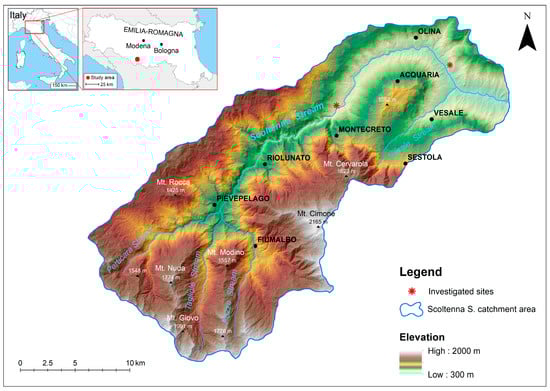
Figure 1.
Location and physiography of the Scoltenna catchment (province of Modena, Italy). The red stars indicate the investigated sites.
2.1. Physical and Climatic Setting
The Scoltenna catchment is located in the Modena Apennines, a fold-and-thrust mountain chain derived from the post-Eocene collisional history between the European and African plates and from a complex, multi-staged evolution [82,83]. Geologically, the area is composed of weak and fractured sedimentary rocks [84]. The main geological formations outcropping in the catchment are calcareous-marly formations in the southern part and clayey formations in the northern part, where the investigated sites are located (Figure 2). According to the regional geological map, the main geological formations outcropping in the Scoltenna catchment are: (i) Monghidoro Formation; (ii) Monte Venere Formation; (iii) Palombini Clays; and (iv) Modena Unit [81].
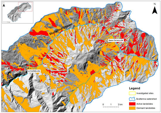
Figure 2.
Landslide map of the lower Scoltenna catchment (Available online: https://geoportale.regione.emilia-romagna.it/ (accessed on 5 July 2023).
The Monghidoro Formation consists of arenaceous-pelitic turbidites with dark grey sandstones that become yellowish brown by alteration and oxidation of femic minerals. The Monte Venere Formation is composed of light grey arenaceous-marly turbidites with thin or medium intervals of dark or blackish clays. The Palombini Clays consist of fissile clays and shale with interspersed medium-to-thick layers of grey calcilutites, usually intensely deformed. The Modena Unit refers to gravel deposits intercalated by sands and silts of alluvial terraces.
The geomorphological features of the Scoltenna catchment result from a series of processes that have been active over a long time (mainly from the Late Pleistocene) in changing climatic and geodynamic conditions. At present, slope instability is the main geomorphological process affecting the Scoltenna catchment, which has been locally obstructed by landslides through time [85]. According to the regional Landslide Map, the geological units show a significant proneness to slope instability [86,87] that is related to the poor mechanical resistance of the outcropping terrains and the presence of groundwater therein. The lithological character of landslide bodies, generally made up of thick clayey deposits with gravels and blocks, is due to the post-failure weathering of claystone, sandstone, and limestone rock fragments. These deposits are in residual strength conditions and, as such, can be quite easily mobilised by slope movements. All landslide types described by Cruden and Varnes [88] can be identified in the study area; however, the most frequent are slow-moving earth slides and earth flows [89,90,91,92,93,94]. According to the Regional Landslide Inventory Map, the lower Scoltenna catchment displays both active and dormant landslides (Figure 2).
The Scoltenna catchment has a Mediterranean climate. Spring and autumn are characterised by intense rainfall, whereas summer and winter are dry with moderate precipitation that sometimes occurs as snowfall [95,96,97]. The average total annual precipitation is 1231.2 mm in the lower Scoltenna catchment and 1915.0 mm in the upper Scoltenna catchment (data recorded in the period 1954–2021) [98]. According to the Köppen classification [99], the present climate of the area is defined as “sub-continental” and locally as “cool-temperate” with a mild temperate climate (Cfa).
2.2. Study Sites
La Confetta and Sasso Cervaro sites are located in the lower Scoltenna catchment. In each site, slope movements have clearly interacted with fluvial morphodynamics through time. La Confetta site is currently affected by an active landslide that is 370 m long and 150 m wide and has an elevation difference of about 80 m and an average slope angle of 12.5° (Table 1 and Figure 3). The substrate consists of arenaceous-pelitic turbidites and clays belonging to the Monghidoro Formation and Palombini Formation. The Sasso Cervaro site is characterised by the presence of an active landslide that is currently 530 m long and 50–60 m wide and has an elevation difference of 160-170 m and an average slope angle of 18.7° (Table 1 and Figure 4). The outcropping terrains consist of clays and shales belonging to the Palombini Formation. From 2019, the whole landslide deposit has been subjected to artificial drainage (Figure 4a).

Table 1.
Morphometry of the La Confetta and Sasso Cervaro sites.
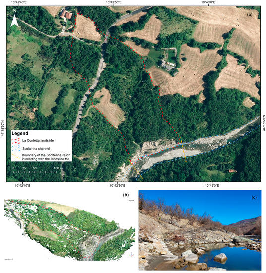
Figure 3.
La Confetta site. (a) La Confetta landslide and related channel reach (orthophoto 2020); (b) 3D model of the site built through the drone photogrammetry performed in 2021; (c) landslide toe and investigated channel reach (2021).
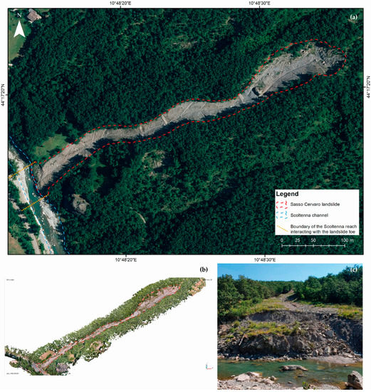
Figure 4.
Sasso Cervaro site. (a) Sasso Cervaro landslide and related channel reach (orthophoto 2020); (b) 3D model of the site built through the drone photogrammetry performed in 2021; (c) landslide toe and investigated channel reach (2021).
At both sites, the activity of the landslides is highlighted by the presence of leaning trees and numerous cracks on the surface of the landslides. The slope movements can be classified as slow-moving earth slides/earth flows and show centimetric movements per year.
The analysed channel reaches at the landslide toe show a length of 120 m at La Confetta site and 60 m at the Sasso Cervaro site and an average slope of 0.9° and 4.7°, respectively. In both reaches, a plane-bed morphology prevails [100] with submerging boulders and cobbles locally organised in oriented lines. Lateral bars are present in both reaches, whereas no pocket floodplains divide the two landslides from the Scoltenna channel; thus, the landslide toes reach the Scoltenna channel, confirming the high potential lateral sediment connectivity in both sites.
3. Materials and Methods
A multidisciplinary approach was used for the investigation of slope and fluvial dynamics, including (i) pre-existing aerial photo and orthophoto collection; (ii) field surveys and geomorphological analysis; (iii) GNSS and photogrammetric surveys; (iv) DEM and orthophoto generation (years 2021 and 2022); (v) multitemporal orthophoto interpretation; and (vi) surface change detection. The research approach and development are illustrated in Figure 5.
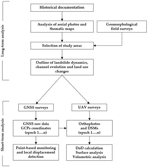
Figure 5.
Workflow of the implemented methodology.
3.1. Data Collection
The two study sites were analysed in a multitemporal perspective through aerial photos and orthophotos available from the Regional Web Map Service [81]. A time span of about 70 years was examined and the following years were considered: 1954, 1977, 1988, 1996, 1998, 2007, 2008, 2011, 2018, and 2020 (Table 2). New orthophotos (3 cm spatial resolution for La Confetta site and 1 cm spatial resolution for the Sasso Cervaro site) were acquired in 2021 and 2022 by means of drone flights (Table 3); two DEMs were obtained for each site with an average point cloud resolution of 0.1 points/cm2 for La Confetta site and 0.3 points/cm2 for the Sasso Cervaro site.
Table 2.
List of examined aerial photos and orthophotos.
Table 3.
Information on survey, photogrammetric processing, and related outputs.
GNSS and UAV photogrammetry surveys were implemented for the monitoring of the investigated landslides. The outputs of the survey campaigns carried out at each site in summers of 2021 and 2022 are discussed. Commercial UAVs and their standard cameras were used: Phantom 4 RTK at La Confetta site and Autel Evo2 at the Sasso Cervaro site. Several crossed flightpaths were planned for each investigated site to guarantee a complete reconstruction and the proper redundancy of images. The flights were planned using an aerial orthophoto and DSM and setting an altitude flight above ground level (a.g.l.) or above sea level (a.s.l.). Moreover, an autonomous mode of image acquisition (with a shot per second and a pseudo-nadiral pose of the camera) was set. Further information about instrumentations, images, and flights is available in Table 3. Artificial targets were positioned in the investigated areas; their positions were measured with a relative rapid static GNSS positioning; the coordinates were then used as GCPs in the SfM processing. The GNSS reference stations were installed in stable positions near the investigated areas. Stonex SC600 and S900A GNSS receivers were used. Some of the GCPs were permanently materialised on the ground in order to be re-measured at each epoch and used as GNSS monitoring points. Each measured baseline had a duration of 10 min and an acquisition rate of 1 Hz. The final accuracy of target coordinates was about 5–6 mm. The photogrammetric targets were wood or PVC numbered plates with a black and white chessboard pattern; the targets are coincident with the GNSS monitoring points incorporated the materialisation of the point.
3.2. Data Processing
The two study sites were analysed in a multitemporal perspective through aerial photos and orthophotos. The multitemporal mapping of landslides and active channels was performed in GIS (ESRI software ArcGis 10.2.1, ArcMap) through a manual delineation method. For each orthophoto in the landslide polygon, the state of activity and land use were mapped; the latter was divided in three classes: woods, bushes, and bare soil.
Active channels in the study reaches were digitised as polygons that included low flow channels and bars (exposed sediments). The average active channel width was evaluated as the ratio between the polygon area and length [101].
Images and ground data acquired on site were processed in Agisoft Metashape to obtain a 3D reconstruction. At the beginning, a quality check of the images was performed in order to delete bad-quality images; then, the relative orientation with high-quality settings was started, and the process was sped up by using the geotag information acquired during the flight. The target locations were manually set up in the acquired images and the coordinate values added to the project. An optimisation of the relative orientation parameters was run to correct errors and obtain georeferenced products. The accuracy of the 3D reconstruction was available at this step. The accuracy is expressed as the discrepancy between the measured and reconstructed coordinates of GCPs; this option is commonly accepted in the absence of validation points [54,65,102]. The values are shown in Table 3. Dense image matching was then performed with high-quality settings; the original images were processed in order to search for pixel-to-pixel correspondences and obtain a 3D dense point cloud. The main output of the photogrammetric processing is the dense point cloud. Additionally, 2D products were obtained starting from the dense cloud, the DEM, and the orthophoto. The processing of La Confetta site led to the generation of DEMs and orthophotos with a resolution of 3 cm; the DEMs generated for the Sasso Cervaro site had a resolution of 2 cm, whereas the orthomosaics had a resolution of 1 cm.
The use of GNSS allowed us to obtain georeferenced results, thus the detection of changes that occurred over time was performed through a direct comparison of the generated products. The DEMs generated at subsequent epochs for each site landslide were compared in a GIS software; QGIS was used in this study. The elevation difference between the same pixel at subsequent epochs was computed; the product is called the DEM of difference (DoD) and allows us to quantify the volume changes. The presence of vegetation affects the volume computation as the terrain surface cannot be detected. In this study, preliminary field surveys allowed the authors to gain knowledge about the investigated sites and to distinguish between vegetated and sparsely vegetated areas. The DoD analysis was performed on the entire sites, but the analyses of the displacements and the calculations of volumes were only performed on sparsely vegetated areas. Other comparison methods were tested, i.e., the comparison between point clouds; however, the results are not reported in this paper because they do not significantly differ from the DoD and are not very effective in volume computation.
In this study, a 3D accuracy value was derived by the discrepancy on GCPs and associated to each generated 3D model. The application of the variance propagation law allowed the estimation of error due to the comparison of the subsequent 3D models. A threshold defining the 95% level of significance was adopted to select reliable displacements.
4. Results
4.1. Long-Term Morphological Evolution of the Investigated Sites
In the 1950s and 1960s, La Confetta landslide was dormant. The landslide was 95% vegetated with woods and bushes covering almost the entire surface. In the 1954 orthophoto, a creek longitudinally crossing the landslide is visible. The Scoltenna Stream presented numerous lateral bars witnessing high sediment transport, and the channel width was approximately 36 m (Figure 6a). From the 1970s until the 2000s, the state of activity did not change significantly: the landslide remained dormant and was covered by woods and crops (Figure 6b).
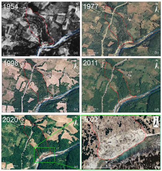
Figure 6.
Morphological evolution of La Confetta landslide through time, outlined by the comparison of orthophotos ranging from 1954 to 2022. The image from 2022 shows the detail of the landslide toe that had been recently reactivated. The red line indicates the boundary of the landslide. The green box indicates the area which is expanded in insert (f).
Although the upper part of the landslide persisted to be dormant, in the 1980s the toe started to activate; the vegetation cover decreased and the toe erosion caused by the Scoltenna Stream became more intense. Fluvial bars appeared on the right side of the stream and the average channel width increased to 39 m. In the 1990s, the upper part of the landslide continued to be rather stable and the landslide toe was less severely affected by toe erosion. As a consequence, the extension of the fluvial bars decreased in size in relation to the progressive stabilisation of the landslide toe (Figure 6c). From the 2000s, the landslide became more active as witnessed, especially in its lower part, by decreased vegetation cover and more widespread bare soil, fluvial processes playing an important role in bank erosion (Figure 6d,e). Figure 6f (from 2022), shows a clear remobilisation of the landslide toe that has caused the displacement of a remarkable volume of sediment into the Scoltenna Stream and the increase in the bars in the channel. As the studied reach is laterally confined, only very limited changes in channel width were observed. In fact, during the whole observation period of 60–70 years, the active channel width ranged between 36 m and 39 m.
During the analysed period, the Sasso Cervaro landslide was characterised by alternating dormant and active phases. In the 1950s and 1960s, the landslide was dormant. It was 70% vegetated and the presence of woods and bushes covering the surface was clearly visible (Figure 7a). The remaining 30% was bare soil, mostly concentrated in the upper part, where the crown developed, and in the middle part. Inside the Scoltenna riverbed, numerous gravel bars were present that were located on both sides of the channel. The channel width was approximately 16 m. In the 1970s and 1980s, the landslide became more active; the regression of the crown was about 15 m and the active surface increased, extending to the middle-lower part of the landslide. The bare soil increased, covering almost 50% of the surface (Figure 7b). By the end of the 1990s, the landslide returned to being dormant; the crown was inactive and the vegetation grew again, covering 60% of the landslide surface (Figure 7c). The same state of activity can be noticed in the 2000s and 2010s when the landslide was 80% vegetated, leaving just 20% of bare soil. From the 1970s to the 2010s, the channel width ranged between 16 and 14 m, and its overall morphology showed no changes. In 2011, the landslide was almost completely covered by vegetation and seemed more stable; the stream, with processes of lateral erosion, caused regression of the landslide toe of about 3 m (Figure 7d). In 2020, the state of activity completely changed, and the bare soil reached 90% of the surface, highlighting an active trend for the landslide (Figure 7e). In Figure 7f, the orthophoto of 2022 shows that the landslide toe advanced and invaded the Scoltenna Stream, causing a displacement of about 4 m of the water flow towards the right side of the riverbank.
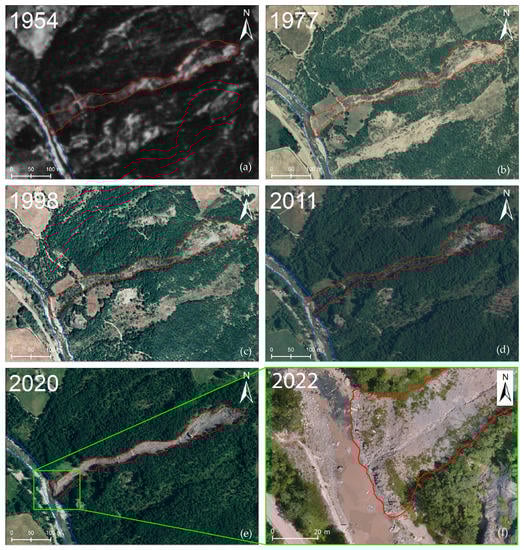
Figure 7.
Morphological evolution of the Sasso Cervaro landslide through time, outlined by the comparison of orthophotos from 1954 to 2022. The image from 2022 shows the detail of the landslide toe. The red line indicates the boundary of the landslide. The green box indicates the area which is expanded in insert (f).
4.2. Short-Term Evolution of the Investigated Sites: Multitemporal Analysis of GNSS Coordinates and Photogrammetric Models
As described in Section 3.2, the products obtained from photogrammetric processing, complemented by GCPs from precise GNSS, exhibit an accuracy to the cm level in the absolute positioning and spatial resolution for both of the investigated sites. The computation of displacements detected with photogrammetric surveys was performed through the direct comparison of the models generated at subsequent epochs. The maps reported below (Figure 8 and Figure 9) represent the DoDs calculated for the investigated sites. The DoDs were calculated as the difference between the second and the first investigated epochs (2022 and 2021, in this study). The DoD analysis allowed the calculation of deposition and erosion volumes that occurred in the investigated period. Positive values indicate an increase in the elevation between the elevation models, thus the deposition of material. Conversely, negative values denote erosion. The volume computation analysis for La Confetta landslide was performed within an area included in the orange polygon represented in Figure 8. La Confetta site exhibits a deposition of 660 m3 at the toe of the landslide and a volume of 190 m3 of sediment eroded by the Scoltenna channel. The computation for the Sasso Cervaro site was focused on the landslide toe and the drainage network. A deposition at the toe of 110 m3 and an erosion on the entire landslide of 213 m3 were detected (Figure 9). The erosional processes are localised inside the artificial drainage network and, due to the activity of the Scoltenna Stream, at the landslide toe.
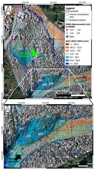
Figure 8.
Map of La Confetta site, displacements computed through DoD (coloured scale) and displacements calculated through GNSS surveys (dots and arrows); (a) view of the entire investigated area; (b) zoom on the landslide toe and channel reach.
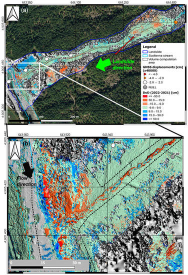
Figure 9.
Map of the Sasso Cervaro site, displacements computed through DoD (coloured scale) and displacements calculated through GNSS survey (dots and arrows); (a) view of the entire investigated area; (b) zoom on the lower part of the landslide and channel reach.
The maps produced (Figure 8 and Figure 9) show accumulation areas represented by blue tones and erosion areas as red tones that correspond to the positive and negative values from the DoD, respectively. The pixels with green colouring, whose values range in the order of ±3.7 cm and ±8.5 cm in La Confetta and Sasso Cervaro, respectively, show vertical displacements that are not significant due to the local statistics reported. The grey colour characterises areas where the absence of data prevents the analysis. Figure 8 and Figure 9 also show the position of the GCPs used to constrain the photogrammetric processing. GCPs permanently materialised on the ground allow the calculation of occurred displacements by comparing the two positions surveyed with GNSS. Displacements are represented with an arrow (horizontal component) and a coloured dot (vertical component); an exaggeration factor was applied for horizontal displacements. The GCPs shown with grey colour (value NULL) were not permanently materialised or their materialisation was lost/damaged during the investigated period.
La Confetta landslide shows significant changes in its lower part, which is in contact with the stream. Elsewhere, the distances calculated with the DoD are smaller and not significant (see the upper-right side of the landslide in Figure 8). The right side of the landslide toe shows positive variations between 15 cm and 50 cm, confirming deposition. The crown area shows vertical displacements ranging between −15 and −4 cm. The GNSS analysis of the detected movements allowed a better characterisation of the changes that occurred during the investigated period. At La Confetta site, the presence of vegetation and the remarkable activity of the landslide did not allow the materialisation of GNSS monitoring points in the toe area. In the GNSS network, points FM53 and FM52 show a subsidence of some centimetres (3–4 cm). The analysis of the GNSS points also provided the computation of the horizontal movements of the landslide: 3 and 5 cm in the south–west direction. These data allowed a better interpretation of the investigated slope processes; further discussion is provided in the following section. In Figure 8a, a focus on the interaction between the slope and the stream is shown, and the results obtained at the landslide toe are reported. At La Confetta site, the deposited materials reduced the channel width of the Scoltenna Stream from 21.5 m (in 2020) to 16.3 m (in 2022) (see Figure 8a). Between 2021 and 2022, although the landslide showed a remarkable deposition (660 m3) and its toe invaded the Scoltenna channel, the stream experienced bed-level lowering between 3 cm and 15 cm in the low-flow channels and stability or very limited aggradation, up to 15 cm, in a few points of the central bar located downstream of the landslide toe. These data do not allow a quantitative analysis, as the accuracy of the photogrammetric models and the significance of DoD, as calculated before, are no longer valid in the presence of water.
The DoD analysis performed on the Sasso Cervaro landslide (Figure 9) did not show significant volume variations, except in the crown area, the drainage network, and at the toe. The detected vertical displacements have a value ranging between −15 and −8.5 cm of removed material. Erosion processes in the artificial drainage channels were recognised, and a deepening of 15–50 cm was calculated. Bank erosion, sliding and consequent deposition were recognised at the foot of the slope (blue and red areas in Figure 9a). The calculated vertical displacements are up to 50 cm in this area. The deposition zone identified in the lower-right part of the landslide is not significant; in fact, values of 15–50 cm could be related to the growth of the grassland. The GNSS monitoring points installed at Sasso Cervaro showed results comparable with those deriving from the DoD analysis: erosion is evident at the landslide crown and toe. The movements calculated through the GNSS monitoring are of 2–4 cm in the elevation and plane components and showed a NE–SW direction. In Figure 9, the horizontal displacements are not visible due to the chosen scale of representation. Point FM02, on the other hand, shows a different behaviour, subsidence of 11 cm and a planimetric displacement of 18 cm according to the landslide direction were detected. As shown in Figure 9a, the landslide toe displays the most significant changes during the investigated period. The right portion of the landslide toe shows intense erosion, whereas the left part shows movements that are not significant for the implemented survey methods. The difference between the material eroded (213 m3) and the material deposited at the toe (110 m3) leads us to think that almost 103 m3 of sediment was transferred to the Scoltenna channel at the Sasso Cervaro site between 2021 and 2022.
5. Discussion
A notable interaction between slope and fluvial dynamics was observed at both investigated sites. The long-term multitemporal analysis of the last 70 years (Figure 6 and Figure 7) showed that when the landslides are more stable and covered by vegetation, the water course plays an important role in the erosion of the landslide toes. On the other hand, when the slopes are more active, the landslides tend to provide sediment to the riverbed.
In La Confetta site, the landslide became more active through time, especially in its lower part. When the vegetation cover decreased and the bare soil became more widespread, fluvial dynamics played an important role in bank erosion processes. Moreover, a remobilisation of the landslide toe caused the displacement of a significant volume of sediment into the Scoltenna Stream (660 m3).
In the Sasso Cervaro site, the landslide showed an intermittent activity through time. When the landslide was almost completely covered by vegetation, the stream caused the regression of the landslide toe due to the processes of lateral erosion. When the landslide was more active, the landslide toe advanced and invaded the Scoltenna Stream, causing a deposition of about 103 m3 of sediment into the riverbed and a displacement of about 4 m of the water flow towards the right side of the riverbank.
The high resolution of the generated products allowed a detailed characterisation of the processes that occurred; in fact, even small features such as boulders and stones could be identified in the DEM. The quantification of small changes, together with variations in topography and slope gradient, was possible. The resolution of the performed analyses is exemplified in the case of La Confetta (Figure 8), where it was possible to identify the uprooted trees and the boulders in the channel (a resolution of 3 cm was achieved). The photogrammetric products have a 3D accuracy of a few centimetres at each epoch (see Table 3). The variance propagation leads to a comparison error of 3.7 cm for La Confetta and 8.5 cm for Sasso Cervaro, these values constituting the threshold for considering the calculated distances as significant with a confidence interval of 95%. The use of a 3D accuracy value for the significance analysis of vertical displacements was precautionary but necessary when comparing DEMs generated from 3D point clouds.
The results shown in the previous section also highlight the accuracy of the photogrammetric products and the performed analyses. In both landslides, stable zones, areas of erosion, and areas of deposition were identified: the crown area and the drainage channels were subject to erosion, whereas at the foot of the slope, deposition can be detected.
The clear and shallow water of the Scoltenna Stream allowed the reconstruction of the riverbed at La Confetta site. Nevertheless, the results of the multitemporal comparison only provided a qualitative evolution of the riverbed during the investigated period. The presence of water refracts the optical rays preventing an accurate and precise 3D reconstruction; specific ground measurements would be necessary to properly model the refraction phenomenon and correct its effects on the riverbed depth computation.
Figure 8 and Figure 9 show good consistency between the displacements calculated with GNSS data on GCPs and DoD; only the vertical component of the GCP displacement was considered for this purpose. The two methods investigated the displacement differently: GNSS provided a punctual analysis of the displacement of a specific point, whereas DoD provided an areal analysis related to the photogrammetric process, the resolution of the point cloud, and the rasterisation process. The two results have different characteristics and genesis but, in the absence of local effects, they should represent the same displacement. DoD analysis allows the identification of processes that show a prevalent effect on the elevation component. DoD is widely used and effective in the monitoring of most landslides when the vertical component of displacements is predominant. There are, however, some displacements for which the horizontal component is also important and requires an integrated use of different surveying and analysis methods.
La Confetta site (see the upper sector in Figure 8) shows the limitations of the DoD analysis: vertical displacements have a small entity and horizontal displacements are predominant and allow a better understanding of the landslide dynamics. In this sector of the landslide, only analysis of GNSS data allowed the computation of displacements.
6. Conclusions
This research analysed the relationships between hillslope processes and the Scoltenna channel dynamics in a long-term (the past 70 years) and a short-term perspective (period 2021–2022). The multitemporal data collected allowed us to assess the morphological evolution of two significant sites in the Northern Apennines and quantify the evolution of surface deformations and volume variations.
The combination of various techniques of remote and proximal sensing used in this study proved to be a useful tool for deciphering the interaction between the investigated slow-moving landslides and fluvial morphodynamics at a suitable resolution and accuracy. In particular, UAV photogrammetry integrated with an accurate GNSS survey proved to be a technique capable of mapping multitemporal changes in the order of a few centimetres per year. Photogrammetry provided high-resolution results that allowed a quasi-continuous detection of the changes that occurred.
Traditional topography techniques provided multitemporal data only on discrete points. However, the use of traditional topography methods is mandatory for the survey of constraint coordinates when high accuracy and repeatable photogrammetric 3D reconstructions are required. The 3D reconstruction and DoD were performed for the whole of the investigated areas, but only the sparsely vegetated portions were considered for the computation of displacements and volumes. Vegetation was not filtered in the original images or final products because this would have resulted in a computed digital terrain model (DTM) with a lower accuracy in the filtered portions, determining a lower confidence.
La Confetta landslide is 370 m long and 150 m wide; the elevation difference is about 80 m. The site was investigated in 2021 and 2022. Vertical displacements up to 3.7 cm were computed at 95% level of significance, and a total of 660 m3 of sediment mobilised into the Scoltenna Stream was detected. The GNSS survey provided errors on the GCP coordinates of about 3–5 mm and allowed a proper coregistation of subsequent 3D reconstructions. In this case, the choice of two different heights of flight (60 m above the entire landslide and 40 m above the foot) allowed the 3D reconstruction of the entire site and a high-accuracy mapping (GSD < 1 cm) of the landslide foot.
In the case study of Sasso Cervaro, a landslide 530 m long and with 170 m of elevation difference was investigated in 2021 and 2022. Vertical displacements up to 8.5 cm/year were detected at 95% level of significance, and a deposition of 103 m3 in the Scoltenna Stream was computed. The detection of highly accurate coordinates for ground targets, together with proper planning of image acquisition, reduced the errors in image orientation and external orientation. A static relative GNSS survey was performed and errors on GCP coordinates were similar to those in La Confetta. In addition, the gridded flightpath followed by the UAV, the off-nadir pose, and the shooting rate ensured a redundancy of images of higher than 90%, a GSD of 1 cm, and strong acquisition geometry. The repeatability of the survey was guaranteed in this study by using the same flight trajectories, shooting frequencies, and processing parameters. In addition, some GCPs were permanently materialised on the ground in order to avoid the effects of a different constraint distribution on the generated 3D point clouds.
The integration of UAV photogrammetry and GNSS is largely used in monitoring applications and proved to be an effective method in landslide investigation. In this paper, it is shown that careful design of the survey and integration of accurate constraints allow a fine-scale investigation of volume changes and surface displacements to evaluate the interaction between slow-moving landslides and fluvial morphodynamics.
Author Contributions
Conceptualisation, C.P., P.R., F.M., V.S. and M.S.; methodology, C.P., P.R., F.M., V.S., F.G. and G.C.; software, C.P., P.R., F.M., V.S., F.G. and G.C.; validation, C.P., P.R., F.M., V.S., F.G. and G.C.; formal analysis, C.P., P.R., F.M., V.S. and G.C.; investigation, C.P., P.R., F.M., V.S., G.C. and M.S.; resources, C.P., P.R., F.M., V.S., F.G. and G.C.; data curation, C.P., P.R., F.M., V.S. and G.C.; writing—original draft preparation, C.P., P.R., F.M., V.S. and F.G.; writing—review and editing, C.P., P.R., F.M., V.S. and M.S.; visualisation, C.P., P.R., F.M., V.S. and M.S.; supervision, F.M. and M.S.; project administration, F.M., F.L. and M.S.; funding acquisition, F.M., F.L. and M.S. All authors have read and agreed to the published version of the manuscript.
Funding
The research presented here has been carried out within the framework of the collaboration between the Inter-Departmental Research and Innovation Centre on Constructions and Environmental Services (CRICT) of the University of Modena and Reggio Emilia and the Regional Agency for Territorial Safety and Civil Protection of Emilia-Romagna, in the frame of the project “Analysis of the interaction between fluvial dynamics and slope processes aiming at the recognition of geomorphological risk situations” (Scientific responsibility: Mauro Soldati).
Data Availability Statement
Not applicable.
Acknowledgments
The authors are grateful to the Regional Agency for Territorial Safety and Civil Protection of Emilia-Romagna and specifically to Edda Pattuzzi for the technical assistance and support. The authors would also like to thank Giada Possemato for her support during field work activities and data processing.
Conflicts of Interest
The authors declare no conflict of interest.
References
- Montgomery, D.R. Process Domains and the River Continuum. J. Am. Water Resour. Assoc. 1999, 35, 397–410. [Google Scholar] [CrossRef]
- Borgatti, L.; Soldati, M. Landslides and Climatic Change. In Geomorphological Hazards and Disaster Prevention; Alcántara-Ayala, I., Goudie, A.S., Eds.; Cambridge University Press: Cambridge, UK, 2010; pp. 87–95. [Google Scholar] [CrossRef]
- Crozier, M.J. Landslide Geomorphology: An Argument for Recognition, with Examples from New Zealand. Geomorphology 2010, 120, 3–15. [Google Scholar] [CrossRef]
- Carlini, M.; Chelli, A.; Vescovi, P.; Artoni, A.; Clemenzi, L.; Tellini, C.; Torelli, L. Tectonic Control on the Development and Distribution of Large Landslides in the Northern Apennines (Italy). Geomorphology 2016, 253, 425–437. [Google Scholar] [CrossRef]
- Cendrero, A.; Remondo, J.; Beylich, A.A.; Cienciala, P.; Forte, L.M.; Golosov, V.N.; Gusarov, A.V.; Kijowska-Strugała, M.; Laute, K.; Li, D.; et al. Denudation and Geomorphic Change in the Anthropocene; a Global Overview. Earth-Sci. Rev. 2022, 233, 104186. [Google Scholar] [CrossRef]
- Micu, M.; Micu, D.; Soldati, M. Mass Movements in Changing Mountainous Environments. In Treatise on Geomorphology; Shroder, J.F., Ed.; Academic Press: Cambridge, MA, USA, 2022; pp. 371–388. [Google Scholar] [CrossRef]
- Picco, L.; Tonon, A.; Ravazzolo, D.; Rainato, R.; Lenzi, M.A. Monitoring River Island Dynamics Using Aerial Photographs and Lidar Data: The Tagliamento River Study Case. Appl. Geomat. 2015, 7, 163–170. [Google Scholar] [CrossRef]
- Turowski, J.M.; Rickenmann, D.; Dadson, S.J. The Partitioning of the Total Sediment Load of a River into Suspended Load and Bedload: A Review of Empirical Data. Sedimentology 2010, 57, 1126–1146. [Google Scholar] [CrossRef]
- Mao, L.; Cavalli, M.; Comiti, F.; Marchi, L.; Lenzi, M.; Arattano, M. Sediment Transfer Processes in Two Alpine Catchments of Contrasting Morphological Settings. J. Hydrol. 2009, 364, 88–98. [Google Scholar] [CrossRef]
- Rainato, R.; Mao, L.; García-Rama, A.; Picco, L.; Cesca, M.; Vianello, A.; Preciso, E.; Scussel, G.; Lenzi, M. Three Decades of Monitoring in the Rio Cordon Instrumented Basin: Sediment Budget and Temporal Trend of Sediment Yield. Geomorphology 2017, 291, 45–56. [Google Scholar] [CrossRef]
- Brierley, G.; Fryirs, K. Geomorphology and River Management: Applications of the River Styles Framework; Blackwell Publishing: Oxford, UK, 2005; 398p. [Google Scholar] [CrossRef]
- Van Asch, T.; Buma, J.; Van Beek, L. A View on Some Hydrological Triggering Systems in Landslides. Geomorphology 1999, 30, 25–32. [Google Scholar] [CrossRef]
- Schuerch, P.; Densmore, A.L.; McArdell, B.W.; Molnar, P. The Influence of Landsliding on Sediment Supply and Channel Change in a Steep Mountain Catchment. Geomorphology 2006, 78, 222–235. [Google Scholar] [CrossRef]
- Brardinoni, F.; Mao, L.; Recking, A.; Rickenmann, D.; Turowski, J.M. Morphodynamics of Steep Mountain Channels. Earth Surf. Process. Landf. 2015, 40, 1560–1562. [Google Scholar] [CrossRef]
- Teng, T.-Y.; Huang, J.-C.; Lee, T.-Y.; Chen, Y.-C.; Jan, M.-Y.; Liu, C.-C. Investigating Sediment Dynamics in a Landslide-Dominated Catchment by Modeling Landslide Area and Fluvial Sediment Export. Water 2020, 12, 2907. [Google Scholar] [CrossRef]
- Scorpio, V.; Cavalli, M.; Steger, S.; Crema, S.; Marra, F.; Zaramella, M.; Borga, M.; Marchi, L.; Comiti, F. Storm Characteristics Dictate Sediment Dynamics and Geomorphic Changes in Mountain Channels: A Case Study in the Italian Alps. Geomorphology 2022, 403, 108173. [Google Scholar] [CrossRef]
- Beylich, A.A.; Brardinoni, F. Sediment Sources, Source-to-Sink Fluxes and Sedimentary Budgets. Geomorphology 2013, 188, 1–2. [Google Scholar] [CrossRef]
- Fryirs, K. (Dis)Connectivity in Catchment Sediment Cascades: A Fresh Look at the Sediment Delivery Problem. Earth Surf. Process. Landf. 2013, 38, 30–46. [Google Scholar] [CrossRef]
- Cavalli, M.; Vericat, D.; Pereira, P. Mapping Water and Sediment Connectivity. Sci. Total Environ. 2019, 673, 763–767. [Google Scholar] [CrossRef] [PubMed]
- Steger, S.; Scorpio, V.; Comiti, F.; Cavalli, M. Data-Driven Modelling of Joint Debris Flow Release Susceptibility and Connectivity. Earth Surf. Process. Landf. 2022, 47, 2740–2764. [Google Scholar] [CrossRef]
- Corsini, A.; Marchetti, M.; Soldati, M. Holocene Slope Dynamics in the Area of Corvara in Badia (Dolomites, Italy): Chronology and Paleoclimatic Significance of Some Landslides. Geogr. Fis. Dinam. Quat. 2001, 24, 127–139. [Google Scholar]
- Li, J.; Cao, Z.; Cui, Y.; Borthwick, A.G. Barrier Lake Formation due to Landslide Impacting a River: A Numerical Study Using a Double Layer-Averaged Two-Phase Flow Model. Appl. Math. Model. 2020, 80, 574–601. [Google Scholar] [CrossRef]
- Li, J.; Cao, Z.; Cui, Y.; Fan, X.; Yang, W.; Huang, W.; Borthwick, A. Hydro-Sediment-Morphodynamic Processes of the Baige Landslide-Induced Barrier Lake, Jinsha River, China. J. Hydrol. 2021, 596, 126134. [Google Scholar] [CrossRef]
- Parenti, C.; Rossi, P.; Soldati, M.; Grassi, F.; Mancini, F. Integrated Geomatics Surveying and Data Management in the Investigation of Slope and Fluvial Dynamics. Geosciences 2022, 12, 293. [Google Scholar] [CrossRef]
- Benda, L.; Hassan, M.A.; Church, M.; May, C.L. Geomorphology of Steepland Headwaters: The Transition from Hillslopes to Channels. J. Am. Water Resour. Assoc. 2005, 41, 835–851. [Google Scholar] [CrossRef]
- Płaczkowska, E. Slope-Fluvial System Structure in the Western Tatra Mountains (Poland): Slope-to-Channel Transition. Arct. Antarct. Alp. Res. 2017, 49, 569–583. [Google Scholar] [CrossRef]
- Krapesch, G.; Hauer, C.; Habersack, H. Scale Orientated Analysis of River Width Changes due to Extreme Flood Hazards. Nat. Hazards Earth Syst. Sci. 2011, 11, 2137–2147. [Google Scholar] [CrossRef]
- Lucía, A.; Comiti, F.; Borga, M.; Cavalli, M.; Marchi, L. Dynamics of Large Wood during a Flash Flood in Two Mountain Catchments. Nat. Hazards Earth Syst. Sci. 2015, 15, 1741–1755. [Google Scholar] [CrossRef]
- Nardi, L.; Rinaldi, M. Spatio-Temporal Patterns of Channel Changes in Response to a Major Flood Event: The Case of the Magra River (Central-Northern Italy). Earth Surf. Process. Landf. 2015, 40, 326–339. [Google Scholar] [CrossRef]
- Thompson, C.J.; Fryirs, K.; Croke, J. The Disconnected Sediment Conveyor Belt: Patterns of Longitudinal and Lateral Erosion and Deposition During a Catastrophic Flood in the Lockyer Valley, South East Queensland, Australia. River Res. Appl. 2015, 32, 540–551. [Google Scholar] [CrossRef]
- Scorpio, V.; Crema, S.; Marra, F.; Righini, M.; Ciccarese, G.; Borga, M.; Cavalli, M.; Corsini, A.; Marchi, L.; Surian, N.; et al. Basin-Scale Analysis of the Geomorphic Effectiveness of Flash Floods: A Study in the Northern Apennines (Italy). Sci. Total Environ. 2018, 640, 337–351. [Google Scholar] [CrossRef]
- Newson, M.D.; Sear, D. The Role of Geomorphology in Monitoring and Managing River Sediment Systems. Water Environ. J. 1997, 11, 264–270. [Google Scholar] [CrossRef]
- Righini, M.; Surian, N.; Wohl, E.; Marchi, L.; Comiti, F.; Amponsah, W.; Borga, M. Geomorphic Response to an Extreme Flood in Two Mediterranean Rivers (Northeastern Sardinia, Italy): Analysis of Controlling Factors. Geomorphology 2017, 290, 184–199. [Google Scholar] [CrossRef]
- Neal, J.; Schumann, G.; Bates, P.; Buytaert, W.; Matgen, P.; Pappenberger, F. A Data Assimilation Approach to Discharge Estimation from Space. Hydrol. Process. 2009, 23, 3641–3649. [Google Scholar] [CrossRef]
- Bishop, M.P.; James, L.A.; Shroder, J.F.; Walsh, S.J. Geospatial Technologies and Digital Geomorphological Mapping: Concepts, Issues and Research. Geomorphology 2012, 137, 5–26. [Google Scholar] [CrossRef]
- Calcaterra, S.; Cesi, C.; Di Maio, C.; Gambino, P.; Merli, K.; Vallario, M.; Vassallo, R. Surface Displacements of Two Landslides Evaluated by GPS and Inclinometer Systems: A Case Study in Southern Apennines, Italy. Nat. Hazards 2012, 61, 257–266. [Google Scholar] [CrossRef]
- Frattini, P.; Crosta, G.B.; Allievi, J. Damage to Buildings in Large Slope Rock Instabilities Monitored with the PSInSAR™ Technique. Remote Sens. 2013, 5, 4753–4773. [Google Scholar] [CrossRef]
- Scaioni, M.; Longoni, L.; Melillo, V.; Papini, M. Remote Sensing for Landslide Investigations: An Overview of Recent Achievements and Perspectives. Remote Sens. 2014, 6, 9600–9652. [Google Scholar] [CrossRef]
- Eker, R.; Aydın, A.; Hübl, J. Unmanned Aerial Vehicle (UAV)-Based Monitoring of a Landslide: Gallenzerkogel Landslide (Ybbs-Lower Austria) Case Study. Environ. Monit. Assess. 2017, 190, 1–14. [Google Scholar] [CrossRef] [PubMed]
- Nikolakopoulos, K.; Kavoura, K.; Depountis, N.; Kyriou, A.; Argyropoulos, N.; Koukouvelas, I.; Sabatakakis, N. Preliminary Results from Active Landslide Monitoring Using Multidisciplinary Surveys. Eur. J. Remote Sens. 2017, 50, 280–299. [Google Scholar] [CrossRef]
- Westoby, M.; Brasington, J.; Glasser, N.F.; Hambrey, M.J.; Reynolds, J.M. ‘Structure-from-Motion’ Photogrammetry: A Low-Cost, Effective Tool for Geoscience Applications. Geomorphology 2012, 179, 300–314. [Google Scholar] [CrossRef]
- Flener, C.; Vaaja, M.; Jaakkola, A.; Krooks, A.; Kaartinen, H.; Kukko, A.; Kasvi, E.; Hyyppä, H.; Hyyppä, J.; Alho, P. Seamless Mapping of River Channels at High Resolution Using Mobile LiDAR and UAV-Photography. Remote Sens. 2013, 5, 6382–6407. [Google Scholar] [CrossRef]
- Wheaton, J.M.; Brasington, J.; Darby, S.E.; Kasprak, A.; Sear, D.; Vericat, D. Morphodynamic Signatures of Braiding Mechanisms as Expressed Through Change in Sediment Storage in a Gravel-Bed River. J. Geophys. Res. Earth Surf. 2013, 118, 759–779. [Google Scholar] [CrossRef]
- Pirot, G.; Straubhaar, J.; Renard, P. Simulation of Braided River Elevation Model Time Series with Multiple-Point Statistics. Geomorphology 2014, 214, 148–156. [Google Scholar] [CrossRef]
- Carlà, T.; Tofani, V.; Lombardi, L.; Raspini, F.; Bianchini, S.; Bertolo, D.; Thuegaz, P.; Casagli, N. Combination of GNSS, Satellite InSAR, and GBInSAR Remote Sensing Monitoring to Improve the Understanding of a Large Landslide in High Alpine Environment. Geomorphology 2019, 335, 62–75. [Google Scholar] [CrossRef]
- Kyriou, A.; Nikolakopoulos, K.; Koukouvelas, I.; Lampropoulou, P. Repeated UAV Campaigns, GNSS Measurements, GIS, and Petrographic Analyses for Landslide Mapping and Monitoring. Minerals 2021, 11, 300. [Google Scholar] [CrossRef]
- Castagnetti, C.; Bertacchini, E.; Corsini, A.; Rivola, R. A Reliable Methodology for Monitoring Unstable Slopes: The Multi-Platform and Multi-Sensor Approach. In Proceedings of the SPIE, Earth Resources and Environmental Remote Sensing/GIS Applications V, Amsterdam, The Netherlands, 23–25 September 2014; Volume 9245, p. 92450J. [Google Scholar] [CrossRef]
- Gili, J.A.; Corominas, J.; Rius, J. Using Global Positioning System Techniques in Landslide Monitoring. Eng. Geol. 2000, 55, 167–192. [Google Scholar] [CrossRef]
- Zeybek, M.; Şanlıoğlu, İ.; Genç, A. Landslide Monitoring with GNSS Measurements and Prediction with Linear Regression Model: A Case Study Taşkent (Konya, Turkey) Landslide. In Proceedings of the Digital Proceeding of the ISDS’2014, Side, Turkey, 10–14 May 2014. [Google Scholar]
- Mantovani, M.; Bossi, G.; Dykes, A.P.; Pasuto, A.; Soldati, M.; Devoto, S. Coupling Long-Term GNSS Monitoring and Numerical Modelling of Lateral Spreading for Hazard Assessment Purposes. Eng. Geol. 2021, 296, 106466. [Google Scholar] [CrossRef]
- Eyo, E.; Musa, T.A.; Omar, K.M.; Idris, K.M.; Bayrak, T.; Onuigbo, I.C.; Opaluwa, Y.D. Application of Low-Cost GPS Tools and Techniques for Landslide Monitoring: A Review. J. Teknol. 2014, 71, 71–78. [Google Scholar] [CrossRef]
- Stark, T.D.; Choi, H. Slope Inclinometers for Landslides. Landslides 2008, 5, 339–350. [Google Scholar] [CrossRef]
- Lane, S.N.; James, T.D.; Crowell, M.D. Application of Digital Photogrammetry to Complex Topography for Geomorphological Research. Photogramm. Rec. 2000, 16, 793–821. [Google Scholar] [CrossRef]
- Rossi, P.; Mancini, F.; Dubbini, M.; Mazzone, F.; Capra, A. Combining Nadir and Oblique UAV Imagery to Reconstruct Quarry Topography: Methodology and Feasibility Analysis. Eur. J. Remote Sens. 2017, 50, 211–221. [Google Scholar] [CrossRef]
- Chudý, F.; Slámová, M.; Tomaštík, J.; Prokešová, R.; Mokroš, M. Identification of Micro-Scale Landforms of Landslides Using Precise Digital Elevation Models. Geosciences 2019, 9, 117. [Google Scholar] [CrossRef]
- Cignetti, M.; Godone, D.; Wrzesniak, A.; Giordan, D. Structure from Motion Multisource Application for Landslide Characterization and Monitoring: The Champlas du Col Case Study, Sestriere, North-Western Italy. Sensors 2019, 19, 2364. [Google Scholar] [CrossRef] [PubMed]
- Godone, D.; Allasia, P.; Borrelli, L.; Gullà, G. UAV and Structure from Motion Approach to Monitor the Maierato Landslide Evolution. Remote Sens. 2020, 12, 1039. [Google Scholar] [CrossRef]
- Lissak, C.; Bartsch, A.; De Michele, M.; Gomez, C.; Maquaire, O.; Raucoules, D.; Roulland, T. Remote Sensing for Assessing Landslides and Associated Hazards. Surv. Geophys. 2020, 41, 1391–1435. [Google Scholar] [CrossRef]
- Meng, Q.; Li, W.; Raspini, F.; Xu, Q.; Peng, Y.; Ju, Y.; Zheng, Y.; Casagli, N. Time-Series Analysis of the Evolution of Large-Scale Loess Landslides Using InSAR and UAV Photogrammetry Techniques: A Case Study in Hongheyan, Gansu Province, Northwest China. Landslides 2021, 18, 251–265. [Google Scholar] [CrossRef]
- Lucieer, A.; de Jong, S.M.; Turner, D. Mapping Landslide Displacements Using Structure from Motion (SfM) and Image Correlation of Multi-Temporal UAV Photography. Prog. Phys. Geogr. Earth Environ. 2014, 38, 97–116. [Google Scholar] [CrossRef]
- Peppa, M.V.; Mills, J.P.; Moore, P.; Miller, P.E.; Chambers, J.E. Accuracy Assessment of a UAV-Based Landslide Monitoring System. ISPRS Int. Arch. Photogramm. Remote Sens. Spat. Inf. Sci. 2016, 41, 895–902. [Google Scholar] [CrossRef]
- James, M.; Robson, S.; D’Oleire-Oltmanns, S.; Niethammer, U. Optimising UAV Topographic Surveys Processed with Structure-from-Motion: Ground Control Quality, Quantity and Bundle Adjustment. Geomorphology 2017, 280, 51–66. [Google Scholar] [CrossRef]
- Casella, V.; Chiabrando, F.; Franzini, M.; Manzino, A.M. Accuracy Assessment of a UAV Block by Different Software Packages, Processing Schemes and Validation Strategies. ISPRS Int. J. Geo-Inf. 2020, 9, 164. [Google Scholar] [CrossRef]
- Pessoa, G.G.; Carrilho, A.C.; Miyoshi, G.T.; Amorim, A.; Galo, M. Assessment of UAV-Based Digital Surface Model and the Effects of Quantity and Distribution of Ground Control Points. Int. J. Remote Sens. 2021, 42, 65–83. [Google Scholar] [CrossRef]
- Agüera-Vega, F.; Ferrer-González, E.; Carvajal-Ramírez, F.; Martínez-Carricondo, P.; Rossi, P.; Mancini, F. Influence of AGL Flight and Off-Nadir Images on UAV-SfM Accuracy in Complex Morphology Terrains. Geocarto Int. 2022, 37, 12892–12912. [Google Scholar] [CrossRef]
- Baum, R.; Messerich, J.; Fleming, R.W. Surface Deformation as a Guide to Kinematics and Three-Dimensional Shape of Slow-Moving, Clay-Rich Landslides, Honolulu, Hawaii. Environ. Eng. Geosci. 1998, 4, 283–306. [Google Scholar] [CrossRef]
- Abellan, A.; Derron, M.-H.; Jaboyedoff, M. “Use of 3D Point Clouds in Geohazards” Special Issue: Current Challenges and Future Trends. Remote Sens. 2016, 8, 130. [Google Scholar] [CrossRef]
- Okyay, U.; Telling, J.; Glennie, C.L.; Dietrich, W.E. Airborne Lidar Change Detection: An Overview of Earth Sciences Applications. Earth-Sci. Rev. 2019, 198, 102929. [Google Scholar] [CrossRef]
- Kakavas, M.P.; Nikolakopoulos, K.G. Digital Elevation Models of Rockfalls and Landslides: A Review and Meta-Analysis. Geosciences 2021, 11, 256. [Google Scholar] [CrossRef]
- Puniach, E.; Gruszczyński, W.; Ćwiąkała, P.; Matwij, W. Application of UAV-Based Orthomosaics for Determination of Horizontal Displacement Caused by Underground Mining. ISPRS J. Photogramm. Remote Sens. 2021, 174, 282–303. [Google Scholar] [CrossRef]
- Mugnai, F.; Masiero, A.; Angelini, R.; Cortesi, I. Integrating UAS Photogrammetry and Digital Image Correlation for Monitoring of Large Landslides. Preprints 2022, 2022010248. [Google Scholar] [CrossRef]
- Al-Rawabdeh, A.; Moussa, A.; Foroutan, M.; El-Sheimy, N.; Habib, A. Time Series UAV Image-Based Point Clouds for Landslide Progression Evaluation Applications. Sensors 2017, 17, 2378. [Google Scholar] [CrossRef]
- Macciotta, R.; Hendry, M.T. Remote Sensing Applications for Landslide Monitoring and Investigation in Western Canada. Remote Sens. 2021, 13, 366. [Google Scholar] [CrossRef]
- Kharroubi, A.; Poux, F.; Ballouch, Z.; Hajji, R.; Billen, R. Three Dimensional Change Detection Using Point Clouds: A Review. Geomatics 2022, 2, 457–485. [Google Scholar] [CrossRef]
- James, M.R.; Robson, S. Mitigating Systematic Error in Topographic Models Derived from UAV and Ground-Based Image Networks. Earth Surf. Process. Landf. 2014, 39, 1413–1420. [Google Scholar] [CrossRef]
- Eltner, A.; Schneider, D. Analysis of Different Methods for 3D Reconstruction of Natural Surfaces from Parallel-Axes UAV Images. Photogramm. Rec. 2015, 30, 279–299. [Google Scholar] [CrossRef]
- Harwin, S.; Lucieer, A.; Osborn, J. The Impact of the Calibration Method on the Accuracy of Point Clouds Derived Using Unmanned Aerial Vehicle Multi-View Stereopsis. Remote Sens. 2015, 7, 11933–11953. [Google Scholar] [CrossRef]
- Wheaton, J.M.; Brasington, J.; Darby, S.E.; Sear, D.A. Accounting for Uncertainty in DEMs from Repeat Topographic Surveys: Improved Sediment Budgets. Earth Surf. Process. Landf. 2010, 35, 136–156. [Google Scholar] [CrossRef]
- Casagli, N.; Frodella, W.; Morelli, S.; Tofani, V.; Ciampalini, A.; Intrieri, E.; Raspini, F.; Rossi, G.; Tanteri, L.; Lu, P. Spaceborne, UAV and Ground-Based Remote Sensing Techniques for Landslide Mapping, Monitoring and Early Warning. Geoenviron. Disasters 2017, 4, 9. [Google Scholar] [CrossRef]
- Nourbakhshbeidokhti, S.; Kinoshita, A.M.; Chin, A.; Florsheim, J.L. A Workflow to Estimate Topographic and Volumetric Changes and Errors in Channel Sedimentation after Disturbance. Remote Sens. 2019, 11, 586. [Google Scholar] [CrossRef]
- Regione Emilia-Romagna. Available online: https://geoportale.regione.emilia-romagna.it/ (accessed on 1 May 2023).
- Bettelli, G.; De Nardo, M.T. Geological Outlines of the Emilia Apennines (Northern Italy) and Introduction to the Formations Surrounding the Landslides which Resumed Activity in the 1994–1999 period. Quad. Geol. Appl. 2001, 8, 1–26. [Google Scholar]
- Cerrina Feroni, A.; Martelli, L.; Martinelli, P.; Ottria, G.; Catanzariti, R. Carta Geologico-Strutturale dell’Appennino Emiliano-Romagnolo alla Scala 1:250,000, (Regione Emilia-Romagna, Servizio Geologico, Sismico e dei Suoli, CNR, Istituto di Geoscienze e Georisorse, Pisa), S.EL.CA., Firenze. 2002. Available online: https://geodata.mit.edu/catalog/mit-q2c4ny27r5jey (accessed on 6 June 2023).
- Abbate, E.; Bortolotti, V.; Passerini, P.; Sagri, M. Introduction to the Geology of the Northern Apennines. Sediment. Geol. 1970, 4, 207–249. [Google Scholar] [CrossRef]
- Soldati, M.; Tosatti, G. Case Histories of Lake-Forming Landslides in the Dragone Valley (Northern Apennines, Italy). In Landslides—Proceedings of the Seventh International Conference and Field Workshop on Landslides in Czech and Slovak Republics; Novosad, N., Wagner, P., Eds.; A.A. Balkema: Rotterdam, The Netherlands, 1993; pp. 287–292. [Google Scholar]
- Bertolini, G.; Canuti, P.; Casagli, N.; De Nardo, M.T.; Egidi, D.; Mainetti, M.; Pignone, R.; Pizziolo, M. Carta della Pericolosità Relativa da Frana della Regione Emilia-Romagna; SystemCart: Rome, Italy, 2002. [Google Scholar]
- Bertolini, G.; Guida, M.; Pizziolo, M. Landslides in Emilia-Romagna region (Italy): Strategies for Hazard Assessment and Risk Management. Landslides 2005, 2, 302–312. [Google Scholar] [CrossRef]
- Cruden, D.M.; Varnes, D.J. Landslide Types and Processes. In Landslides: Investigation and Mitigation; Turner, A.K., Shuster, R.L., Eds.; Transportation Research Board; National Research Council: Washington, DC, USA, 1996. [Google Scholar]
- Ronchetti, F.; Borgatti, L.; Cervi, F.; Lucente, C.C.; Veneziano, M.; Corsini, A. The Valoria Landslide Reactivation in 2005–2006 (Northern Apennines, Italy). Landslides 2007, 4, 189–195. [Google Scholar] [CrossRef]
- Trigila, A.; Iadanza, C.; Bussettini, M.; Lastoria, B.; Barbano, A.; Munafò, M. Dissesto Idrogeologico in Italia: Pericolosità e Indicatori di Rischio. Rapporto 2015, 233, 2015. [Google Scholar]
- Bertolini, G.; Corsini, A.; Tellini, C. Fingerprints of Large-Scale Landslides in the Landscape of the Emilia Apennines. In Landscapes and Landforms of Italy. World Geomorphological Landscapes; Soldati, M., Marchetti, M., Eds.; Springer: Cham, Switzerland, 2017; pp. 215–224. [Google Scholar] [CrossRef]
- Mulas, M.; Ciccarese, G.; Ronchetti, F.; Truffelli, G.; Corsini, A. Slope Dynamics and Streambed Uplift during the Pergalla Landslide Reactivation in March 2016 and Discussion of Concurrent Causes (Northern Apennines, Italy). Landslides 2018, 15, 1881–1887. [Google Scholar] [CrossRef]
- Piacentini, D.; Troiani, F.; Daniele, G.; Pizziolo, M. Historical Geospatial Database for Landslide Analysis: The Catalogue of Landslide Occurrences in the Emilia-Romagna Region (CLOCkER). Landslides 2018, 15, 811–822. [Google Scholar] [CrossRef]
- Ciccarese, G.; Mulas, M.; Alberoni, P.P.; Truffelli, G.; Corsini, A. Debris Flows Rainfall Thresholds in the Apennines of Emilia-Romagna (Italy) Derived by the Analysis of Recent Severe Rainstorms Events and Regional Meteorological Data. Geomorphology 2020, 358, 107097. [Google Scholar] [CrossRef]
- Tomozeiu, R.; Busuioc, A.; Marletto, V.; Zinoni, F.; Cacciamani, C. Detection of Changes in the Summer Precipitation Time Series of the Region Emilia-Romagna, Italy. Theor. Appl. Climatol. 2000, 67, 193–200. [Google Scholar] [CrossRef]
- Tomozeiu, R.; Lazzeri, M.; Cacciamani, C. Precipitation Fluctuations during the Winter Season from 1960 to 1995 over Emilia-Romagna, Italy. Theor. Appl. Climatol. 2002, 72, 221–229. [Google Scholar] [CrossRef]
- Pavan, V.; Tomozeiu, R.; Cacciamani, C.; Di Lorenzo, M. Daily Precipitation Observations over Emilia-Romagna: Mean Values and Extremes. Int. J. Climatol. 2008, 28, 2065–2079. [Google Scholar] [CrossRef]
- Agenzia Prevenzione Ambientale Energia Emilia-Romagna. Available online: https://www.arpae.it/ (accessed on 1 May 2023).
- Köppen, W. Grundriß der Klimakunde, 2nd ed.; Walter de Gruyter and Co.: Berlin, Germany; Leipzig, Germany, 1931. [Google Scholar]
- Montgomery, D.R.; Buffington, J.M. Channel-Reach Morphology in Mountain Drainage Basins. GSA Bull. 1997, 109, 596–611. [Google Scholar]
- Surian, N.; Rinaldi, M.; Pellegrini, L. Linee Guida per l’analisi Geomorfologica Degli Alvei Fluviali e Delle loro Tendenze Evolutive; Cooperativa Libraria Editrice Università di Padova: Padova, Italy, 2009; 79p. [Google Scholar]
- Mancini, F.; Castagnetti, C.; Rossi, P.; Dubbini, M.; Fazio, N.L.; Perrotti, M.; Lollino, P. An Integrated Procedure to Assess the Stability of Coastal Rocky Cliffs: From UAV Close-Range Photogrammetry to Geomechanical Finite Element Modeling. Remote Sens. 2017, 9, 1235. [Google Scholar] [CrossRef]
Disclaimer/Publisher’s Note: The statements, opinions and data contained in all publications are solely those of the individual author(s) and contributor(s) and not of MDPI and/or the editor(s). MDPI and/or the editor(s) disclaim responsibility for any injury to people or property resulting from any ideas, methods, instructions or products referred to in the content. |
© 2023 by the authors. Licensee MDPI, Basel, Switzerland. This article is an open access article distributed under the terms and conditions of the Creative Commons Attribution (CC BY) license (https://creativecommons.org/licenses/by/4.0/).