Article

A New Blind Selection Approach for Lunar Landing Zones Based on Engineering Constraints Using Sliding Window

1
College of Geoexploration Science and Technology, Jilin University, Changchun 130026, China
2
Institute of Integrated Information for Mineral Resources Prediction, Jilin University, Changchun 130026, China
3
Institute of Geochemistry, Chinese Academy of Sciences, Guiyang 550081, China
4
State Key Laboratory of Lunar and Planetary Sciences, Macau University of Science and Technology, Macau 999078, China
5
Key Laboratory of Lunar and Deep-Space Exploration, National Astronomical Observatories, Chinese Academy of Sciences, Beijing 100101, China
6
School of Astronomy and Space Science, University of Chinese Academy of Sciences, Beijing 100049, China
*
Author to whom correspondence should be addressed.
Remote Sens. 2023, 15(12), 3184; https://doi.org/10.3390/rs15123184
Submission received: 9 May 2023 / Revised: 13 June 2023 / Accepted: 17 June 2023 / Published: 19 June 2023

Abstract

:
Deep space exploration has risen in interest among scientists in recent years, with soft landings being one of the most straightforward ways to acquire knowledge about the Moon. In general, landing mission success depends on the selection of landing zones, and there are currently few effective quantitative models that can be used to select suitable landing zones. When automatic landing zones are selected, the grid method used for data partitioning tends to miss potentially suitable landing sites between grids. Therefore, this study proposes a new engineering-constrained approach for landing zone selection using LRO LOLA-based slope data as original data based on the sliding window method, which solves the spatial omission problem of the grid method. Using the threshold ratio, mean, coefficient of variation, Moran’s I, and overall rating, this method quantifies the suitability of each sliding window. The k-means clustering algorithm is adopted to determine the suitability threshold for the overall rating. The results show that 20 of 22 lunar soft landing sites are suitable for landing. Additionally, 43 of 50 landing sites preselected by the experts (suitable landing sites considering a combination of conditions) are suitable for landing, accounting for 90.9% and 86% of the total number, respectively, for a window size of 0.5° × 0.5°. Among them, there are four soft landing sites: Surveyor 3, 6, 7, and Apollo 15, which are not suitable for landing in the evaluation results of the grid method. However, they are suitable for landing in the overall evaluation results of the sliding window method, which significantly reduces the spatial omission problem of the grid method. In addition, four candidate landing regions, including Aristarchus Crater, Marius Hills, Moscoviense Basin, and Orientale Basin, were evaluated for landing suitability using the sliding window method. The suitability of the landing area within the candidate range of small window sizes was 0.90, 0.97, 0.49, and 0.55. This indicates the capacity of the method to analyze an arbitrary range during blind landing zone selection. The results can quantify the slope suitability of the landing zones from an engineering perspective and provide different landing window options. The proposed method for selecting lunar landing zones is clearly superior to the gridding method. It enhances data processing for automatic lunar landing zone selection and progresses the selection process from qualitative to quantitative.

1. Introduction

As human knowledge of the Moon deepens and evidence increases for the potential presence of water ice and near-surface volatiles in polar regions, a new competition for lunar exploration has been initiated. China National Space Administration (CNSA), NASA, European Space Agency (ESA), Russian Federal Space Agency (ROSCOSMOS), Lunar and Planetary Institute (LPI), Japan Aerospace Exploration Agency (JAXA), Indian Space Research Organization (ISRO), and many other organizations have developed plans for future exploration of the Moon [1,2,3,4,5,6,7]. In order to clarify the conceptual framework of lunar exploration and guide scientific progress in lunar exploration, Ouyang [8], Scientific Context for Exploration of the Moon [9], Lunar Exploration and Analysis Group (LEAG) [10], European Space Agency [4,11], etc. have presented the main scientific concepts for lunar exploration. This can be summarized in eight propellable scientific concepts [12]. Manned landings on the lunar surface, in situ exploration, and sample return are the most efficient ways to advance the study of the scientific concepts of the Moon. These concepts include the history of thermal evolution, the thickness of the lunar crust, the internal structure, the history of impacts, the characteristics of volatile fractions in the lunar polar regions, and the available resources of the lunar surface [13].
So far, 22 soft lunar landings have been successful, including those by the Luna, Surveyor, Apollo, and Chang’E (CE) projects [14,15,16,17,18]. The success of these missions depends mainly on the choice of landing zones. As a result, research into landing zone selection can help the landing mission fulfill its scientific goals while simultaneously ensuring the probe’s safe landing. Since the development of lunar exploration, many scholars, domestic and abroad, have constrained the selection of landing zones for lunar missions from both engineering and scientific standpoints. These decisions generally follow the principles of technical feasibility, achievable scientific goals, and unique scientific objectives [19,20,21]. In this way, they suggest landing sites that are conducive to the advancement of lunar landing missions. For example, the CE-3 mission is the first Chinese lunar landing mission focusing on space engineering capabilities to select five candidate landing sites on the lunar near side [22]. Ultimately, Sinus Iridum was selected as the landing site based on CE-3 scientific and engineering constraints because of its significant advantages, including suitability for lunar-based astronomical observations, relatively flat terrain, and facilitation of smooth communications and temperature control [23]. With the development of space technology capabilities, CE-4 is more oriented toward the lunar far side. Nine candidate landing regions were selected to explore shallow structures on the lunar far side [24]. After selecting engineering constraints, including topographic slope, terrain obstacles (craters, rocks, and boulders), communication conditions, and temperature, the Von Kármán crater in the northern SPA basin was selected as the CE-4 landing site. It is the first rover to land and rove on the lunar far side [20,25]. The region of the lunar near-surface at about 43° latitude is ideal for measurements and communications, according to CE-3’s experience. Second, young lunar sample collection was a goal of the CE-5 mission [26]. Combining the aforementioned two points, CE-5, China’s first lunar sample return mission, selected the zone around Mons Rümker’s relatively young geological age. In successive CE missions, the selection of landing zones resulted from a balancing act between scientific objectives that provided the vital impetus to studying fundamental scientific concepts such as lunar geological dating [27,28], volcanic activity, and thermodynamic evolution. Simultaneously, engineering considerations were considered to ensure the spacecraft’s safety and the scientific mission’s accomplishment [29].
Traditional landing zone selection methods currently use expert knowledge to manually analyze and scientifically evaluate, score, and rank potential landing zones to achieve their goals. Originally, expert knowledge for landing zone selection revolved around screening based on geological features [30,31], topography [32,33], composition [34], and internal structure [35]. As scientific concepts advanced and technologies for deep space exploration matured, a selection of scientific significance was gradually made. Jawin et al. [12] summarized recent progress in the Lunar Science for Landed Missions workshop, e.g., volcanism, the formation of impact craters and basins, and lunar water ice. Considering scientific topics such as impact crater formation processes and dating, volatiles, volcanism, magnetism, geophysics, and astrophysics, these topics describe many high-priority options for lunar surface landing sites. Xiao Long [36] recommended 18 alternative landing sites, focusing on lunar geological issues such as the composition of the deep lunar crust and mantle, mantle structure, impact fluxes, volcanic thermal evolution, lunar resources, and the environment. Bound H2O, or frozen water ice, occurs mainly in the permanently shadowed regions of the Moon in the southern and northern polar regions. In contrast, subsurface solid H2O could occur in a wider area than these shadowed areas [37]. As a result, the research on the lunar polar regions has attracted widespread attention. CE-6, CE-7, CE-8, Luna-25, Luna-27, and Chandrayaan-2 [1,3,33,38] focused on the water ice in the lunar polar region and other potential cold-capture volatiles and selected suitable sites with potential scientific results. Using high-precision lunar polar data, including LOLA 5 mpp (m per pixel), 1 mpp DEMs, LROC 20 mpp NAC, etc., the Environmental Systems Research Institute (ESRI) [39] analyzed craters in ArcGIS and identified six promising locations in Sverdrup that contain multiple regions of spatially dense ice. In June 2019, NASA [40] selected the SIMPLEx mission Lunar Trailblazer to purposefully measure the infrared properties of the lunar surface. Mission objectives are to detect and map water on the lunar surface at key targets to determine its form, assess possible time-variation in lunar water on sunlit surfaces, map the form, abundance, and distribution of water ice in the PSRs, and conduct reconnaissance for candidate landing sites. Guangfei Wei et al. [41] presented the concept of the Chinese Chang’e-7 (CE-7) lunar polar exploration mission. They calculated the illumination rate for partial coverage of Shackleton Crater in the lunar southern summer. They recommended one part of the Shackleton Crater rim as the main landing site for the CE-7’s sunlit area and cold trap explorations. The traditional approach can be summarized as the concentration of scientific content and location preference of potential regions. However, the selection process with expert knowledge is very time-consuming [42] and lacks effective models for quantifying the assessment.
In recent years, with the development of big data and machine learning, researchers have explored cost-effective quantitative modeling algorithms to automate the selection of landing zones [43]. To create an evaluation model for landing zones, Zeng and Mu [34] proposed a multifactor weighted ranking model to automatically calculate and visualize the suitability of a landing zone. Jia et al. [44] proposed a fuzzy analysis design selection model that uses fuzzy inference methods to determine candidate landing site evaluation metrics that can evaluate alternative landing zones with multiple engineering constraints based on available data. Daison et al. [45] used a coalescent hierarchical clustering approach to classify different lunar landforms identified with Lunar Reconnaissance Orbiter (LRO) Wide Angle Camera (WAC) data. They then applied trajectory constraints to narrow down the number of potential landing sites. To establish an effective model to evaluate the whole Moon from a quantitative perspective for intelligent optimization, Cao and Wang et al. [46] proposed the automatic optimization of landing zone selection using a weight-of-evidence and fractal approach. For the automatic selection of landing zones, two issues must be considered: (1) the lack of overlap in the whole-Moon grid cut results in missing space in the grid boundary; (2) it is difficult to calculate the appropriate index of the landing zone for any area at any location by the quantitative model of the weight-of-evidence and fractal method.
Sliding windows can process large data sets by decomposing the data into smaller and partially overlapping windows to analyze the data while improving computational performance [47,48]. Furthermore, because of its variable step size, it may more thoroughly cover the range of grid borders that the grid approach neglects, offering a simple and efficient solution. The landing zone should be able to provide a smooth and safe geographic area for the probe’s soft landing and the probe’s work while considering the safety requirements of spacecraft and scientific instruments [12]. During the rocket-supported landing process, the slope affects its propellant loss and the insignificance of the collision when it touches the lunar surface. On the other hand, during the descent of a rover on a slope while driving on the surface, the slope also affects the safety of the rover’s route. Major bumps can jeopardize the rover’s operation [1]. Therefore, the suitability or unsuitability of the slope is often the first consideration in selecting the landing zones as the primary evaluation condition [3,12,33,44]. Previous methods for selecting landing zones to quantify slope data consisted mainly of the average slope and the slope percentage below a certain threshold (threshold ratio) [21,22,30]. However, slope data should be considered in the following three aspects when selecting a suitable landing site: (1) The average slope data in the selected range should be low, and the percentage of slope that is below the threshold should be high; (2) the dispersion of the slope data in the selected range should be more stable; (3) the spatial characteristics of the slope data in the selected range should have high aggregation characteristics. The mean slope and threshold ratio only consider the first aspect. Therefore, in this study, the coefficient of variation and Moran’s I [49] are used to evaluate and quantify the dispersion and aggregation characteristics of the data. The hierarchical analysis method is used to construct a comprehensive quantitative index for the slope range suitable for landing. The threshold value for evaluating whether a location is acceptable for landing is established using the k-means approach (unsupervised learning’s most popular clustering algorithm).
In summary, this study adopts the sliding window method to solve the spatial omission problem in the grid method by taking advantage of the overlap and variables. The coefficient of variation and Moran’s I are introduced based on the threshold ratio and mean slope. It evaluates the dispersion and spatial distribution characteristics of single-window slope data, visually quantifies the suitability of single-window landing zones, and realizes a landing zone preference method based on engineering constraints.

2. Materials and Methods

2.1. LOLA Data Introduction and Pre-Processing

The Lunar Reconnaissance Orbiter (LRO) [50] was launched to the Moon at 5:32 p.m. EDT on 18 June 2009 [51]. The Lunar Orbiter Laser Altimeter (LOLA) was carried aboard the Lunar Reconnaissance Orbiter [52]. It uses short pulses of a solid-state laser through a diffractive optical element (DOE) to make four types of measurements: the distance between the spacecraft and the lunar surface, the energy of the laser pulse reflected from the lunar surface, the width of the returned laser pulse, and the solar radiation reflected from the lunar surface. These basic measurements obtained results such as topography, laser wavelength, roughness of the lunar surface, and solar reflectance [52].
The LRO Digital Elevation Model (DEM) integrates more than 6.5 billion measurements collected between July 2009 and July 2013 [53]. The elevation results achieved a high accuracy of 60 m at 256 pixels per degree over the whole lunar region.
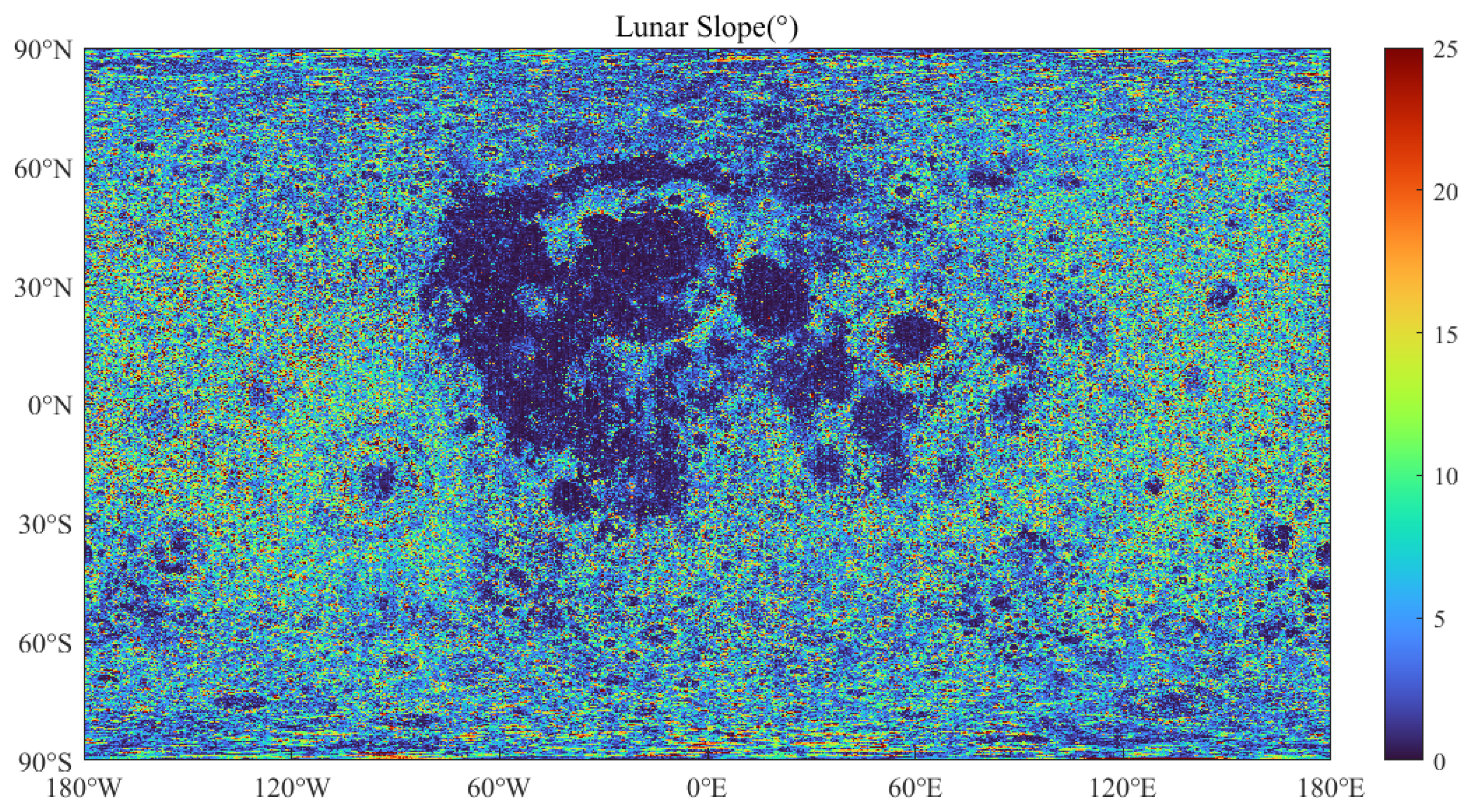
As shown in Figure 1, terrain slope indicates the steepness of the surface terrain. In DEM raster data, a pixel is usually combined with eight adjacent pixels to form a slope. The slope is calculated by dividing the elevation difference from east to west by the elevation difference from north to south [54]. The equation used to calculate the slope of pixel “e” is as follows:
d z / d x = [ ( c + 2 f + i ) ( a + 2 d + g ) ] / ( 8 × L ) ,
d z / d y = [ ( g + 2 h + i ) ( a + 2 b + c ) ] / ( 8 × L ) ,
S = tan 1 ( d z / d x ) 2 + ( d z / d y ) 2
where a–i represents the elevation of each pixel, L represents the size of the pixel, dz/dx represents the slope in the east–west direction (x), and dz/dy represents the slope in the north–south direction (y). The slope of “e” is the arc tangent of the square root of the sum of the squares of the two slopes. S represents the slope. A slope map of the whole Moon was obtained based on the DEM data and the above equation [55]. It is shown in Figure 2. Figure 2 shows the slope of the whole Moon with a horizontal resolution of 512 pixels per degree (60 m at the equator) and a typical vertical accuracy of 3 to 4 m. The DEM has a horizontal resolution of 5.5 m per degree. Approximately 90% of the DEM pixels show root mean square vertical residuals of less than 5 m. In addition, geolocation errors using LOLA altimetry profiles are typically 10 m horizontally and 1 m vertically [56].

2.2. Methods

2.2.1. The Sliding Window Principle

An array of data with a defined window size is subjected to the requested operation using the sliding window algorithm, which loops across the data in the desired direction. The sliding window algorithm performs the requested operation on an array of data with a specified window size and loops across the data in the specified direction. It provides a flexible and powerful way to process the data in a structured and efficient manner [48]. The method is applied to landing zone selection using a sliding window to move and analyze two-dimensional whole Moon slope data (a remote sensing image of the slope) row by row and column by column. Finally, the method provides areas suitable for landing in terms of engineering aspects. The method can cut out the whole Moon grid without limiting the operation. Therefore, it can reduce the complexity of the landing zone suitability assessment problem.
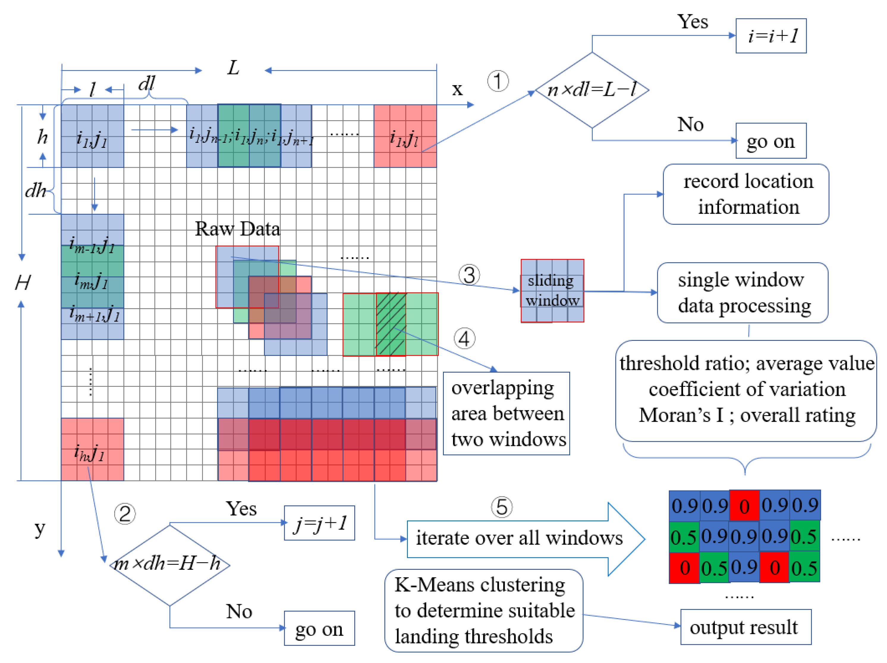
The schematic diagram of the sliding window algorithm is shown in Figure 3. The diagram includes the original data’s total length, L, and the total width, H. Additionally, it showcases the window length, l, and the window width, h. The diagram also highlights the sliding step, dl, in the direction of window length and the sliding step, dh, in the direction of window width. Here, im and jn represent the window length and width direction indexes, respectively. The basic content includes the following parts:
  • Selecting the window size: The first step in using sliding windows is to select the window size that contains the number of data points in each window, depending on the specific problem to be solved and the properties of the data set. During the landing zone selection process, the choice of window size depends mainly on the purpose of the landing site. For example, if the purpose is to build a lunar base, a larger area is needed to accommodate the site selection; if the purpose is for a lander landing, the smaller the window size, the better with high-resolution data.
  • Window slide: Once the window size is selected, the window begins to slide into the dataset within a specified increment. The distance between each slide is called the step size and determines the degree of overlap between successive windows. This is shown in Figure 3 ④.
  • Sliding termination condition: When sliding lengthwise, as in Figure 3 ①, the window slides from the beginning of the next line if the product of the column index and lengthwise step is equal to the difference between the data length and the window length; correspondingly, when sliding widthwise, the decision condition is as in Figure 3 ②. If both ① and ② are satisfied, it means that the traversal cycle of the original data is complete, and the sliding is terminated.
  • Data analysis: As the windows move through the data set, each window is analyzed independently. Independent analysis of the windows includes recording the window position information and processing the data from each window. Data processing includes statistics and the calculation of the average slope, threshold ratio, coefficient of variation, Moran’s I, and overall rating.
  • Output generation: When the sliding of the original data is completed, as shown in Figure 3 ⑤, each window already contains the corresponding index, which results in the output. The output results represent the summary statistics of each window, or a set of features extracted from the slope data, to generate the landing zone selection results in the form of a matrix or surface elements. “Surface elements” means the area corresponding to the window size is contained in surface elements. For example, the attributes of a 1° × 1° window size include the composite indicator within the window as well as the 30.3 × 30.3 km2 area and range filled by that window. In the rendering process, a k-means clustering algorithm is used to determine the appropriate thresholds for landing.

2.2.2. Threshold Ratio

The threshold ratio, defined as the ratio between the number of pixels smaller than a given threshold and the total number of pixels, is used to evaluate the flatness of slope data. It is the most commonly used metric for evaluating slopes in landing zones [23].
S = p ( < t h r e s h o l d ) / P
where S represents the threshold percentage, p(<threshold) represents the number of pixels in the window less than the threshold, and P represents the total number of pixels in the window.
Previous studies assumed that the average terrain slope of the landing zones should not exceed 8° [1,21,29]. In the initial selection of candidate landing regions, it was assumed that an average slope of less than 20° would be suitable for the rover’s landing and roving [33]. Therefore, 8° and 20° were chosen as the thresholds for selection.

2.2.3. The Coefficient of Variation

The coefficient of variation provides a method for comparing the variability of data with different means and is a useful tool in the process of data analysis [57]. The coefficient of variation, Cv, is introduced to quantify the amount of scatter in slope data. It can be calculated by standard deviation, σ,/mean, μ.
C v = σ μ
A too-large average slope does not correspond to safe landing conditions in the landing zones and leads to a higher average value and, thus, a lower coefficient of variation. In addition, the threshold of 8° is more uniformly distributed than the threshold of 20°, so the raw data from the single window are binarized according to the threshold of 8°. The data that is below the threshold (flatter) is set to 1, and vice versa, to 0.

2.2.4. Moran Index

The Moran Index (Moran’s I) was devised by Moran [58] to measure geographic autocorrelation. Evaluations of the spatial distribution characteristics of the data, whether the data are spatially aggregated or discrete, employ the Moran Index, with Moran’s I value distributed in [−1, 1]. In this range, [0, 1] denotes a positive correlation between geographical units, [−1, 0] denotes a negative correlation, and 0 denotes no correlation. The formula is as follows:
I = n S 0 j = 1 n j = 1 n w i , j z i z j i = 1 n z i 2
where zi is the deviation of the element’s attribute from its mean (xi − X), wi,j is the spatial weighting between elements i and j, n is the total number of elements, and S0 is the aggregation of all spatial weightings:
S 0 = i = 1 n j = 1 n w i , j
For the spatial matrix, wi,j, the spatial weight matrix is introduced based on Queen proximity. Queen proximity refers to defining neighboring locations or areas based on a specific criterion. When creating a spatial weight matrix, the concept of queen proximity involves considering all adjacent or neighboring locations as connected, as shown in Figure 4. The Queen proximity cell of cell “A” is cell “B”, which contains the common vertex connection and common adjacent edge connection.
Assuming that the boundary points, i, of the spatial cell are represented by bi, the spatial weight matrix based on the proximity of Queen is calculated as in Equation (8).
w i , j = { 1 , b i b j 0 0 , b i b j = 0

2.2.5. Overall Rating and Factor Weights

From the standpoint of landing safety, we intended to choose a window suitable for landing that provided the four benefits listed below: (1) the mean value inside this window’s slope data is low, which meets the basic criterion that the lander can land safely; hence, the mean value was chosen for evaluation; (2) the percentage of low slope within this window’s slope data should be high, indicating that this window offers a wide range of safe landing terrain; hence, the threshold ratio was chosen. (3) there are fewer high anomalies in this window’s slope data, which reduces the risk of landing in areas with abrupt terrain changes, so the coefficient of variation is chosen; (4) the low values of slope data in this window have spatial aggregation characteristics, which ensure the spatial continuity of safe landing terrain. While the threshold ratio may not capture the degree of dispersion or spatial characteristics, the Moran index is chosen. Since each indicator has its drawbacks, the threshold ratio, defined as the ratio between the number of pixels smaller than a given threshold and the total number of pixels, cannot evaluate the degree of dispersion and spatial characteristics of the data. Additionally, the coefficient of variation does not consider the spatial distribution characteristics of the data. Moran’s I can only assess the spatial aggregation of the same attribute values of the data (spatial distribution). When the high value of the data is aggregated with the high value, its value will be higher than that of the aggregation of low value and low value. Therefore, the Analytic Hierarchy Process (AHP) was introduced to provide ideas for weighing multiple indicators for selecting landing zones on the slope.
AHP has been widely used in many fields, such as natural resource management, regional planning, environmental impact assessment [59,60], and the study of lunar science [61]. The AHP breaks down the problem into various constituent factors according to the nature of the problem and the overall goal to be achieved. It assembles the factors at various levels according to their mutual influences and affiliations and forms a multilevel analytical structural model. Thus, the problem becomes focused on determining the relative weights or relative advantages and disadvantages of the lowest level (options, measures, etc., for decision-making) in relation to the highest level (the overall goal) [62].
Five parameters, such as threshold ratio (8), threshold ratio (20), mean slope, coefficient of variation, and Moran’s I are used to construct a comprehensive index for evaluating the suitability of landing zones. It includes three dimensions to quantify flatness: data mean, data dispersion, and data spatial distribution characteristics. To quantify the parameters’ significance, the slope data’s dispersion and spatial distribution characteristics are considered according to the Saaty scale of 1–9 (see Table 1) [62].
The weights are determined as follows: Moran’s I measures the spatial distribution properties of the data, with a value of 1 classified as important when high values are clustered with high values. Additionally, while the slope dispersion tends to affect the safety of the landing zone, the coefficient of variation becomes more important, and the quantified value of importance is 5. In the initial check of the landing zone, an average slope of less than 20° is safe for landing and roving the probe [33]. However, because it extends the threshold boundary, a more fundamental determinant of landing zone selection, landing zone safety is quantified to a lesser degree and is considered of low importance, with a quantified value of 3. Considering that threshold ratio versus average slope is commonly used to evaluate slope in previous literature and that the average terrain slope of the landing zone should not exceed 8°, the area with a slope of less than 8° should account for a relatively large percentage [1,21,29]. Subsequently, it was found that the threshold ratio (8) and the average slope with a quantitative value of 7 were equally important. The judgment matrix was constructed as shown in Table 2.
The consistency evaluation of the judgment matrix is an essential step in applying the hierarchical analysis method, and the principal eigenvalue (λmax) represents a function of the dispersion of the matrix consistency [64]. The pairwise matrix is considered consistent if λmax is greater than or equal to the number of constructed layers (5 layers), and the principal eigenvalue is calculated as 5.1127. To check the consistency of the normalized weights, the consistency ratio (CR) is used. The consistency test is regarded as passed if the consistency ratio (CR) is equal to or less than 10%. To calculate the consistency ratio (CR), the consistency index (CI) formula was introduced as follows [65]:
C I = λ max n n 1
where λmax denotes the principal eigenvalue and n denotes the number of parameters. Here, the CI is 0.028181. The consistency ratio (CR) is then calculated according to the following equation:
C R = C I R I ( n )
The random consistency index RI represents the random index given in Table 3 for different values of n. Here, the RI for the five parameters (n = 5) equals 1.12, and the CR is 2.5%.
Of these, a 2.5% (less than 10%) CR was allowed for a weighted overlay analysis to integrate the weighted parameters of the composite metrics for the landing zones. The final overall rating, Q, is derived as follows:
Q = 0.3632 * M e a n + 0.3632 * R a t i o ( 8 ) + 0.076652 * R a t i o ( 20 ) + 0.15782 * ( 1 C v ) + 0.039119 * M o r a n I
To normalize the overall rating, when the average slope is less than 8°, the mean value is 1, and vice versa, it is 0.

2.2.6. K-Means Clustering Algorithm

For the quantitative results of the landing zones, it is still necessary to determine the threshold value to distinguish the interval range of suitable or unsuitable values for landing. The k-means algorithm is characterized by its fast calculation and good clustering performance, and it is also the most popular classification method [15,67,68] that has been widely used in lunar research [69]. The k-means clustering method is an unsupervised learning algorithm that divides a dataset into k clusters based on the similarity of the dataset. The algorithm works by iteratively assigning data points to the closest cluster center (centroid) and then updating the centroid based on the new assignment. This process is repeated until the assignment converges and the center of mass no longer changes [70].
One of the challenges of using k-means clusters is determining the appropriate value of k, which indicates the number of clusters. If the value of k is too low, the algorithm will attempt to group the data into fewer clusters than are actually there. This can cause separate clusters to merge, resulting in the loss of valuable information. However, if the value of k is chosen too high, the algorithm will attempt to construct more clusters than necessary. This might result in excessive data fragmentation, resulting in small and perhaps unimportant clusters. The expectation that sample points within each class have high similarity and sample points between classes have low similarity is often achieved by minimizing the sum of the squares of the errors from each sample point within a class to the class midpoint [71]. The elbow method is commonly used for determining this value, which selects the best k value by plotting the sum of squares within the cluster (WCSS) as a function of the following values, k [72]. Using the error sum of squares as the objective function for clustering includes the sum of the squared distances between each data point and its assigned center of mass. Multiple runs of k-means resulted in several different sets of clusters. As the number of classifications k increases, so does the number of clustering centers. As more clustering centers are assigned to the same data, the original data becomes closer to the clustering centers, and the WCSS decreases. Beyond a certain point, the decrease in WCSS becomes less significant. Consequently, the plot of WCSS as a function of k begins to exhibit an “elbow” shape. This characteristic allows for the plotting of WCSS for different values of k, enabling visual inspection of the elbow points to determine the optimal value of k. The overall flow of the k-means clustering algorithm is as follows [73]:
In the sample data set:
( D = { ( x 11 , x 12 , , x 1 T ) , , ( x M 1 , x M 2 , , x M T ) } )
Set k clustering centers, which means the sample set is divided into k classes; T is the number of data features to assign M sample point values to each of the initial clustering centers:
( μ 1 ( 1 ) , μ 2 ( 1 ) , , μ k ( 1 ) )
Find the minimum distance of Pt with respect to μ i ( j ) and assign Pt to the class with the minimum distance with respect to μ i ( j ) to update the clustering center of each class:
μ i ( j + 1 ) = 1 M i P i t
The squared error Ei is calculated for all points in the data set, D, and compared with the previous error comparison, Ei−1.
E i = i = 1 k t = 1 M i | P i t μ i j + 1 |
If |Ei+1 − Ei| < δ, the algorithm terminates, and the error sum of squares at that k value is recorded; otherwise, it continues with the next iteration. After the completion of the iteration, multiple k values are substituted to represent the WCSS for different k values and determine the optimal number of classifications. Data results from multiple indicators in the landing zones are clustered using the k-means algorithm, and the smallest value in the data class with the largest center of mass is selected as the threshold for evaluating the suitability of the landing zones.

3. Results

The whole lunar slope obtained using DEM data processing [56] undergoes a series of steps, including sliding window traversal and a single window evaluation based on multiple indicators such as threshold ratio, average value, coefficient of variation, Moran’s I, and overall rating. These processes represent the results of automatic landing zone preference in the following three ways: (1) the quantification of whole-Moon results of landing zone suitability by the sliding window method; (2) the local comparison between the sliding window method and the grid method; and (3) the evaluation of the candidate landing regions.

3.1. Quantitative Results of Whole Moon Slope Evaluation

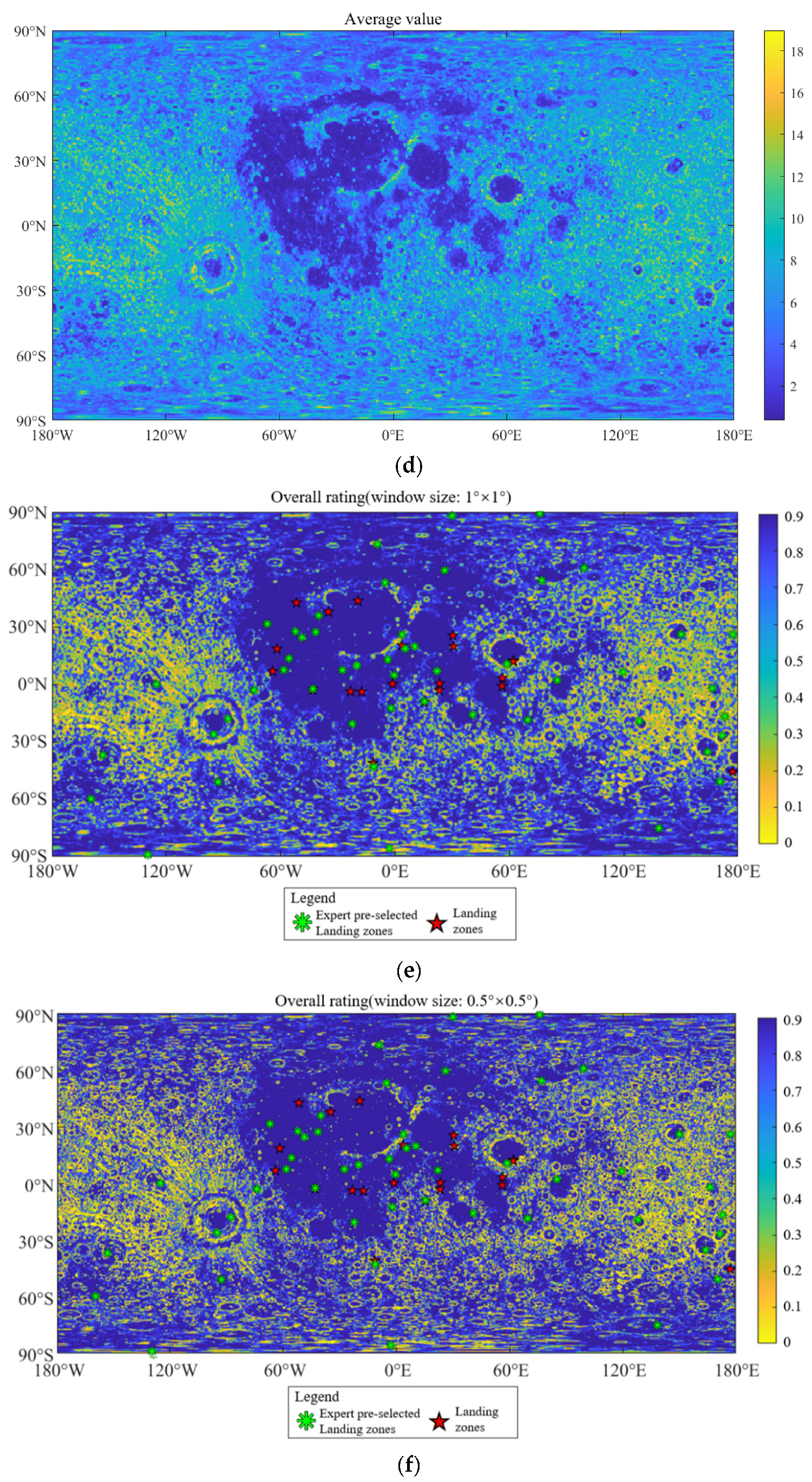
When selecting the landing zones, considering a slope based on the sliding window method for the whole Moon, the size of the single window is set to 1° × 1° (actual range: 30.3 cosφ km × 30.3 km, φ is the latitude), 0.5° × 0.5°. The same movement step in both directions is set to 0.5° and 0.25°, respectively. Additionally, 359 × 719 and 719 × 1439 windows are obtained with overlap from the corresponding window rating index database. The quantitative scores of each window were aggregated for the whole Moon, and the results of the whole Moon slope evaluation varied for different indicators (Figure 5).
Figure 5a–f shows the quantitative scoring results of the whole-Moon slope threshold ratio (20), threshold ratio (8), coefficient of variation, average value, and overall rating, respectively. The composite evaluation results in Figure 5f are overlaid with the successful soft landing sites (red pentagons) and the landing sites preselected by the experts (green snowflakes).
The results in Figure 5 show a consistent general trend. The blue areas suitable for landing are all on the flat lunar mare and at the bottom of the large impact craters, reflecting the lunar topography and landscape better. This is consistent with the perception that the bottom of the lunar mare and the large impact craters are flatter [46]. Second, the quantification of the threshold ratio (20) in Figure 5a shows that the blue area suitable for landing is too wide relative to other results in Figure 5b–f. Furthermore, the average slope of the whole Moon is 6.23°, as shown by the statistics of the 258,123 windows obtained by the sliding window method. The total number of windows with a threshold ratio (20) less than 0.8 is only 3922, which is 1.5% of the total number of windows, highlighting the scattering of the unsuitable areas. This explains the scattered distribution of yellow areas in Figure 5a. In addition, the results of Moran’s I tend to produce higher values for areas where high values are clustered with high values and lower values for areas where low values are clustered with low values. However, the overall range of Moran’s I is between [−1, 1], and the minimum value of Moran’s I for the whole Moon is more than 0.7, indicating that the slope has strong spatial autocorrelation properties. It can strictly constrain the overall rating scores considering the spatial characteristics of the slope data, which can be seen in Figure 5e.
Based on the comparison of the results of Figure 5f (overall rating), Figure 5c (coefficient of variation), Figure 5b (threshold ratio (8)), and Figure 5d (mean), it can be concluded that the suitable landing range has an incremental variation characteristic. However, this pattern does not apply to the central lunar mare region of the Moon, which remains constant. This is determined by the properties of the slope data in the window. If the slope data are concentrated in a 1° window containing 256 × 256 pixels at values below 8° in the lunar mare, the result will be suitable for landing. If the data are concentrated in the window at values above 8° in the highland region, the result will not be suitable for landing. Suppose there are data “anomalies” that are much higher than the average value in the border area between the lunar mare and the highlands, and the coefficient of variation is more sensitive to this situation than the average value and the threshold percentage indicator. In that case, the coefficient of variation will increase, affecting the results of the composite indicator. This is consistent with the Surveyor 3 assessment results in Table 4, where the mean slope and threshold ratio metrics are acceptable. Still, the coefficient of variation is inadequate, leading to the conclusion that the Surveyor 3 one-window is not suitable for landing. However, determining the suitable landing range is rather subjective, and it is impossible to objectively determine the range of suitable landing indicators. The association between the range of values in the blue area and the degree of landing suitability is determined by the color bar of the resulting map. The application of the scientific method is needed to provide a scientific explanation. The numerical range of the overall rating suitable for landing can be provided for the classification of the window. Therefore, the k-means clustering algorithm determines the interval of each suitable indicator for landing. The best classification scheme for different window sizes is shown in Figure 6.
Figure 6 shows that the degree of distortion measured by WCSS improves significantly when k = 3, since image degradation is no longer significant after that. The optimal number of clusters is 3 for both the window sizes of 1° and 0.5°. For a window size of 1° × 1° and 0.5° × 0.5°, the data class prime of the overall rating is 0.93, 0.79, 0.27, 0.93, 0.70, and 0.17, respectively. Therefore, the thresholds of 0.81 and 0.77 for the overall rating were chosen to determine the appropriate landing criteria for the two window sizes.
Among them, 38 of the 50 preselected landing sites were within the interval at a window size of 1°, corresponding to 76%. At a window size of 0.5°, 43 landing sites were within the interval, corresponding to 86%. A comparison between Figure 5e,f shows that the blue range suitable for landing is wider in Figure 5f. This feature is more evident in the highlands because the window area covered by the smaller window size is smaller, and the slope is less hilly in the geomorphological features of the highlands and impact craters. Therefore, the smaller window size is more suitable for the landing zone preference scheme, consistent with experts’ pre-selection of the landing zone statistics.
The sliding window method was used to create a whole Moon database containing the location information of each window, corresponding indices, and multiple evaluation metrics. To evaluate the quantification effect of the whole Moon slope and demonstrate the database effect, Table 4 lists the various evaluation metrics of the soft landing sites more directly.
Table 4 lists several evaluation metrics for the successful 22 soft landing sites. Since the sliding window motion step is half the window size, each landing site is contained in four windows, reflecting the following characteristics: (1) the maximum average slope of the previous landing sites was 11.08° for Apollo 17. With a window size of 1° × 1°, the average inclination of all landing sites is 3.7°. (2) Since each landing site corresponds to four windows, the highest value among the four windows is used as the overall rating for the landing site. With a window size of 1° × 1°, the number of landing windows above the threshold of 0.81 determined by k-means clustering is counted. There are 20 landing site windows in total, which is 90.9%. The total number of windows below the threshold is 12. For a window size of 0.5° × 0.5°, the number of landing site windows meeting the threshold of 0.77 is 20, which is 90.9%. The total number of windows below the threshold is 10. Among the landing site windows that scored lower than the overall score threshold, Luna 20 (Apollonius Plateau in Mare Fecunditatis), Surveyor 7 (Tycho), Apollo 15 (Montes Apenninus) and Apollo 17 (Taurus–Littrow) are landing sites that are different from general landing sites on the lunar mare and are more focused on scientific objectives. Special terrains such as highlands, canyons, and mountains were chosen to ensure the mission’s safety and smooth operation, which explains their lower overall rating [17,74]. Surveyor 3 landed within the impact crater Surveyor, which is a small crater that was subsequently named after the mission. This impact crater is situated at the Mare Cognitum of southeastern Oceanus Procellarum. It is worth noting that the Mare Cognitum has a significant slope ripple that surrounds the impact crater Surveyor in a semicircle and extends to another impact crater Head, resulting in a higher coefficient of variation and a lower overall rating [15]. Therefore, the overall rating provides a better quantitative level for evaluating previous soft landing sites.

3.2. Comparison of Sliding Window and Grid Method

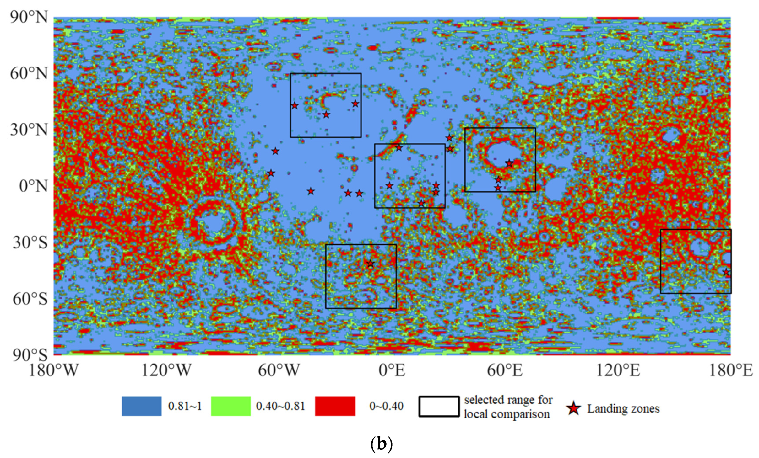
The grid method referred to here is different from the grid method that focuses on the areal distribution of various surface morphology features in the planetary surface analysis [75], but rather a fishing net cut approach that deals with raster data. The purpose is to grid the data in order to make the individual data more standardized for statistical purposes. To compare the differences between the grid method and the sliding window method, the size of the single window was set to 1° × 1°. The step size of the grid method was equal to the window size, and the step size of the sliding window method was set to 0.5° in both directions. This resulted in 179 × 359 grids without overlap and 359 × 719 windows with overlap. The overall rating was then classified using the k-means cluster method. The optimal number of classifications for the grid method is set to 3 according to the WCSS and the error inflection point, and the classification intervals are set to 0.81 and 0.40, respectively. The final results are output in the form of surface elements to obtain the results of evaluating the whole Moon slope based on the grid method and the sliding window method (Figure 7).
The results in surface elements (Figure 7) differ from the output results in matrix form in Figure 5 in that each window and grid contain the corresponding area. The comparison shows that the preferred results of the landing zones calculated by the sliding window are more detailed than those of the conventional grid method. Specifically, the sliding window method provides a larger spatial range of suitable landing sites in the central lunar mare region and the high-latitude highland region. The adjacent part between the grids contains the spatial area not included in the operation, and the sliding window’s overlapping characteristic extracts the grid method’s central area and merges it from there. The unsuitable landing zones in the raster method become more suitable for landing, and the newly formed suitable landing zones are smoother and more natural, making the transition more distinct.
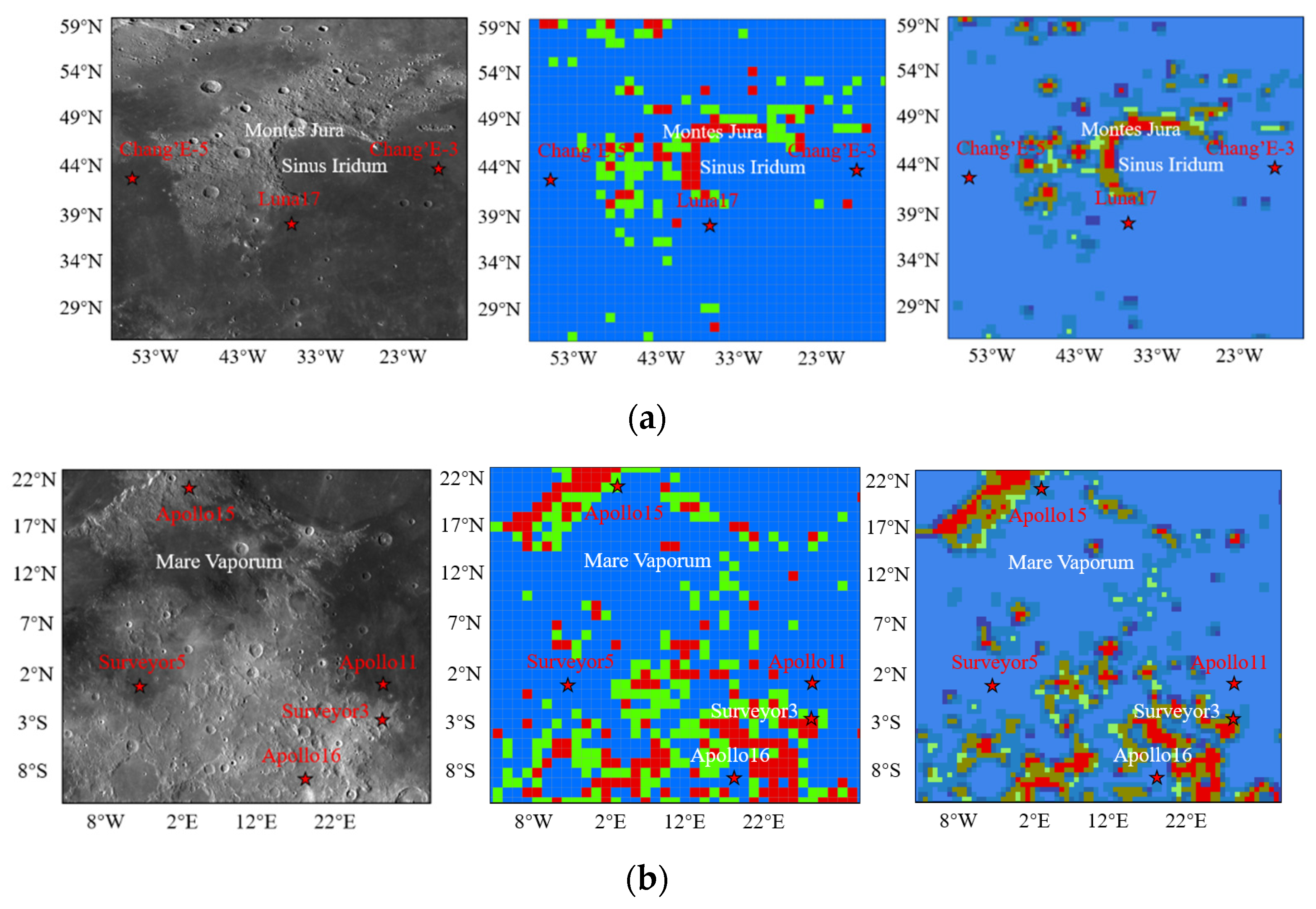
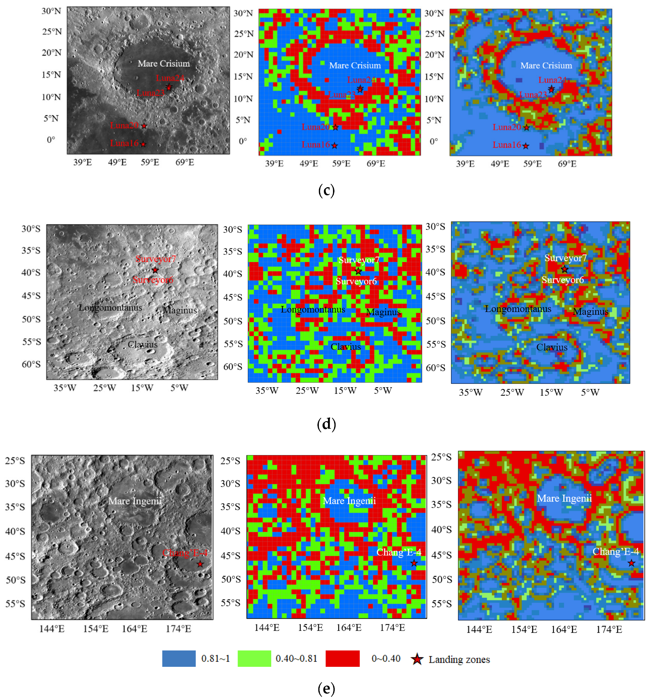
To compare the local differences between the grid and the sliding window methods, geomorphic terrains such as the boundary of the lunar mare, highlands, mountains, and impacts were selected as study areas. The lunar place names and soft landing sites were locally magnified and overlaid to obtain Figure 8.
The results in Figure 8 show the local differences between the grid and sliding window methods. Figure 8a is located in the Sinus Iridum rainbow bay and the Jura Mountains in the northwestern part of Mare Imbrium, including the landing sites CE-3 and CE-5. The results of the grid and sliding window methods show that there are a wide range of suitable landing spaces in Mare Imbrium. At the same time, the Jura Mountains and the scattered impact areas are unsuitable for landing because of the greater differences in slope. Figure 8b, located in Mare Vaporum, contains five landing sites, including Apollo 11, 15, and 16, and Surveyor 3 and 5. The grid method results show that two landing sites, Surveyor 3 and Apollo 15, are not suitable for landing, while the sliding window method results show that they are suitable for landing. The regional spatial distribution of suitable landing sites is continuous, except for the highlands in the south, the mountains, and the impact crater terrain in the north. Figure 8c is located in Mare Crisium, which contains four landing sites: Luna 16, 20, 23, and 24—all suitable for landing. The unsuitable landing space is distributed in a circular pattern, consistent with the geomorphology. Figure 8d is located in the Tycho impact, in the southern highlands of Mare Nubium, where Surveyors 6 and 7’s landing sites are located. It is evident that two landing sites are suitable for landing in the sliding window method results but not in the grid method results, which reflects the completeness of the sliding window method for data evaluation. Figure 8e, located at the Von Kármán impact crater, contains the landing site CE-4, which is suitable for landing according to the slope estimation results. The geomorphology surrounding it is more clearly outlined in the sliding window method results than in the grid method results.
In general, Figure 8a–e all contain soft landing sites, and the suitable landing zones of the grid method results are also considered suitable for landing from the sliding window method results. However, the landing zones unsuitable for the grid method, such as in Figure 8b Surveyor 3, Apollo 15, and Figure 8d Surveyor 6, 7, fall into the suitable landing zones of the sliding window method results. This is consistent with the conclusion that only Luna 20 and Apollo 17 are unsuitable for landing based on the slope evaluation in Table 4. Second, the differences are primarily reflected in the lunar mare boundaries, impacts, mountains, and other geomorphic terrain. The sliding window method evaluates the area between grids to make the transition between the overall assessment classification results smoother and complement the grid method’s spatial omissions.

3.3. Evaluation of Lunar Candidate Landing Regions

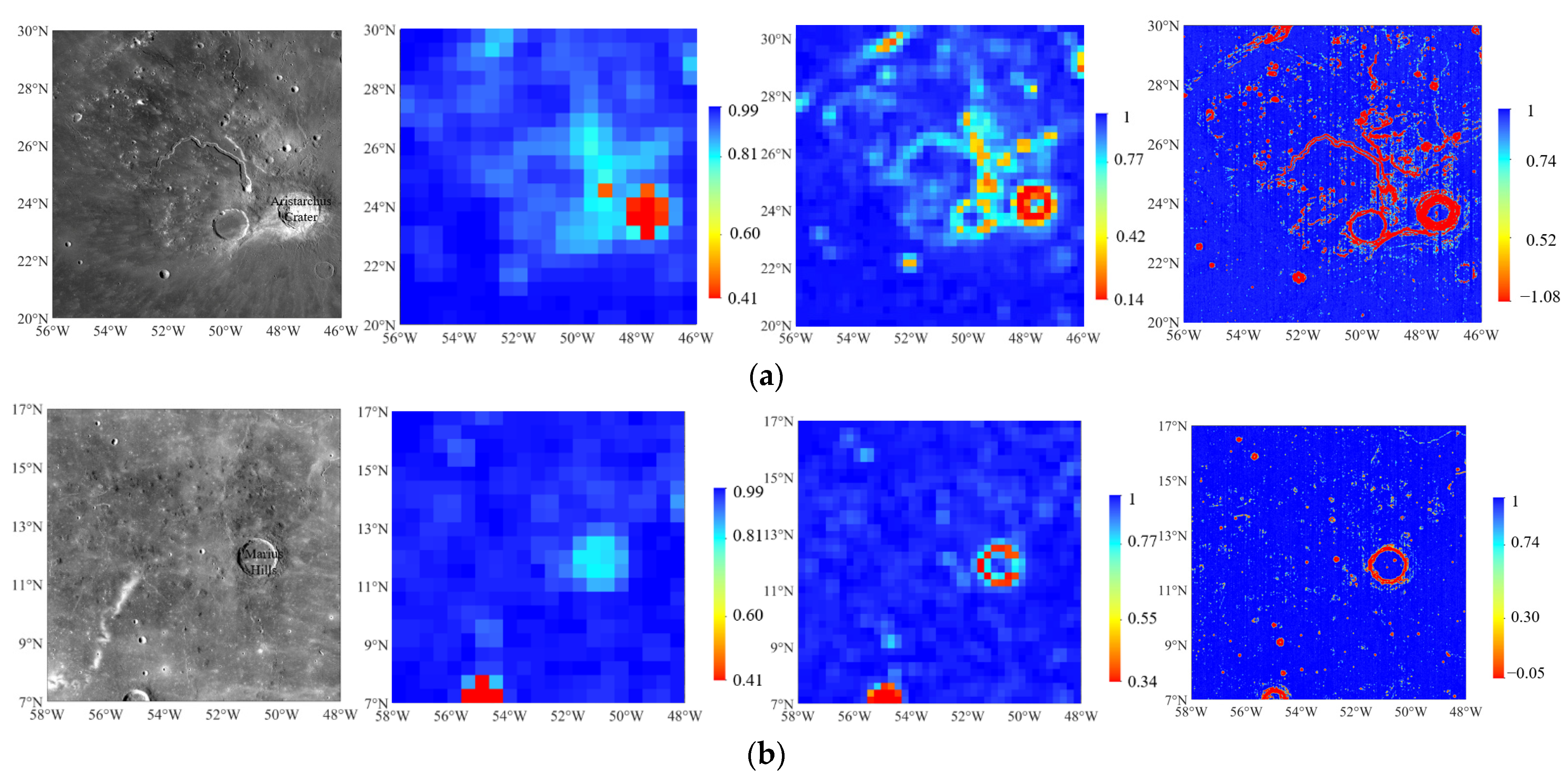
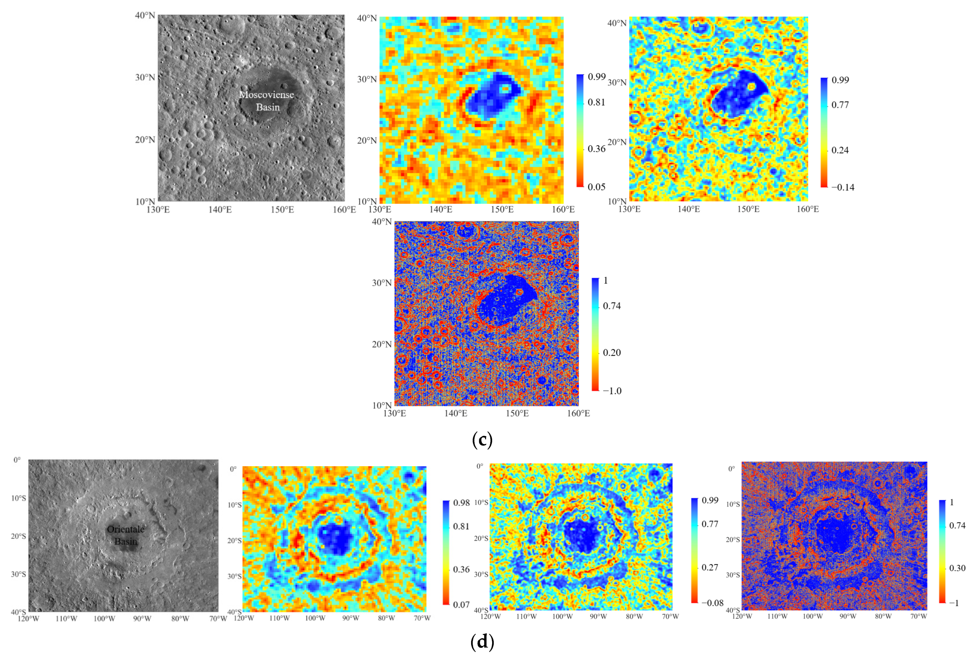
Lunar candidate landing regions are recommended jointly by Jawin et al. [12] and Xiao Long et al. [36]. There are four identical landing sites: two on the lunar near side (Aristarchus Crater and Marius Hill) and two on the lunar far side (Moscoviense Basin and Orientale Basin). For the obtained integrated index of the slope, the results are output in matrix form to obtain Figure 9. With a window size of 1° × 1°, 0.5° × 0.5°, and 0.03125° × 0.03125°, the suitable landing zones according to the k-means clustering algorithm are in the range of 0.81~1.00, 0.77~1.00, and 0.74~1.00, respectively.
Aristarchus Crater, located on the Aristarchus Plateau, was formed during the Copernican period and had a central position of 23.7°N, 312.6°E, and a diameter of 40 km. The Aristarchus plateau contains the largest pyroclastic deposit, the widest and deepest sinuous rille, and relatively young basalts immediately adjacent to the plateau [76,77]. Its young formation history has resulted in less erosion and later alteration, with layered rock outcrops on its central peak and crater walls [78]. The presence of Mare Imbrium ejecta could excavate lunar mantle material. Therefore, as a landing site, Aristarchus Crater may provide new insights into scientific questions about volcanism, the primitive products of magma ocean differentiation [78], and the composition of the deep Moon.
The results in Figure 9a show the suitable areas for landing at Aristarchus Crater and the surrounding area considering the slope, with the percentage of suitable areas in the different window sizes being 92%, 94%, and 90%, respectively. The unsuitable areas at the bottom of Aristarchus Crater increase with decreasing window sizes. The degree of landing evaluation for the sinuous rille with linear features can also reflect the suitable landing area.
Marius Hills lie in the middle of the Oceanus Procellarum and contain mare basalt units of varying composition, centered at 13.3°N, 306.8°E. There are a large number of volcanic constructions (domes, cones, meandering Moon streams, lava flows, etc.) [79,80], and the ages of the different basalt units vary widely, with young basalts being rich in olivine [81]. Therefore, as a landing site, Marius Hills can advance scientific questions about complex and long-lasting volcanism, olivine outcrops, and basalt units.
The results in Figure 9b reflect the suitable landing areas in Marius Hills and nearby areas, considering the slope. Figure 9b shows that the candidate area has a wide range of suitable landing zones for different window sizes, with the suitable landing area percentages being 99%, 98%, and 97%, respectively. The suitable landing areas can be evaluated for small window sizes, even if the impact is small. The impact craters, such as those around Marius Hills, are shown as red circles in the last column of Figure 9b (due to the small window size assessment) and are not shown in the third column of Figure 9b.
Moscoviense Basin is a multiring impact basin of Nectarian age [82], centered at 27.2°N, 147.6°E. The basin contains the thinnest crust on the Moon, mare deposits, pyroclastic deposits, and lunar swirls. It is geologically diverse and contains gorthopyroxene, olivine, and Mg–Al spinel. The composition of a lunar mare within the basin is highly variable, and the interior of the basin has undergone multiple magma fillings [83]. Therefore, scientific knowledge about the Moon that can be obtained as a landing site includes magnetic anomalies of the lunar swirls, the geologic age, structure, and composition of the lunar far side basin, evidence of heat flows in the thinnest region of the lunar crust, and the tectonic features of the high-density lunar mare basalt.
The results in Figure 9c reflect the suitable landing areas in the Moscoviense Basin and adjacent regions considering the slope, with the percentage of suitable landing windows in different window sizes being 17%, 26%, and 49%, respectively. The increase in the area of the candidate landing regions makes the combined indices at large window sizes also reflect good identification.
Orientale Basin is the youngest and best-preserved multiring basin on the Moon, centered at 20.0°S and 265.0°E and containing three concentric rings with more than 20 mare ponds. The ejecta of the basin is divided into three distinct units, of which the Maunder Formation is considered to be ancient primary Orientale ejecta material [84]. Possible scientific discoveries at this landing site include valid constraints on the dating curve of impact craters, information on KREEP rocks, access to lower lunar crust or even lunar mantle material, and information on pyroclastic deposits or ancient lunar mare samples [85].
The results in Figure 9d show the suitable areas for landing in Orientale Basin and adjacent areas considering slope, with the percentage of suitable areas being 21%, 37%, and 55%, respectively. The evaluation results for different window sizes show that the central part of the Orientale Basin is suitable for landing. At the same time, the areas between the concentric rings are also increasingly suitable for landing from large to small window sizes. Table 5 shows the overall assessment results for the four candidate landing regions mentioned above.
From Table 5 and comparisons with Figure 9, it can be concluded that the difference in the preselected area of the candidate zone affects the evaluation of the overall rating metrics. The suitable landing areas of Aristarchus Crater, Marius Hills, and Orientale Basin are greater than 50%, and the suitable landing area of Moscoviense Basin is 49% with a small window size of 0.03125° × 0.03125°. For the Aristarchus Crater and the Marius Hills on the lunar near side, the small impacts and sinuous rille contained in them are difficult to estimate by the overall assessment for a large window size when the preselected landing area is small. For the Moscoviense Basin and Orientale Basin, when the landing area is large, the large window size has obvious differences in evaluating the suitability of the landing area for various landform features. The small window size can finely evaluate the suitability of the landing area with the advantage of a large number of windows (3,682,561 and 8,186,241 windows were involved in the assessment, respectively). This approach increases the area of the candidate regions suitable for landing, especially in the region of transition from high to low slope. Consequently, there is a gradual increase in the area ratio of large windows to small windows, which explains the higher results of the small window evaluation for Moscovien Basin and Orientale Basin in Table 5. Therefore, the overall evaluation proposed in this paper can constrain the suitability range of the landing area from the engineering perspective of slope and quantify the suitability degree of the landing area within the range.

4. Discussions

Although the method proposed in this paper can obtain a spatial region suitable for landing on the whole Moon with slope-oriented constraints in any area and range, there are still two possible problems that need to be improved:
  • The sliding window method causes all pixel points to participate in the operation more than once. The evaluation index in the range of the whole Moon needs 30 h to complete the calculation with a window size of 1° × 1° and a step size of 0.5°, which takes more than three days when each window is cut and presented. For the 10° × 10° candidate landing zones, the required computation time for all window sizes is about 150 s, which is still not sufficient even for evaluating the safety of the probe’s lunar surface landing site slope during descent. The required computation time is relatively long, and optimized calculation methods such as distributed computing and high-performance computing may need to be used to increase the computation speed.
  • This study only confirms the effectiveness of this method; hence, it only analyzes slopes with an engineering boundary condition. The amount of rock [86,87], the roughness of the lunar surface, the lighting conditions, the polar terrain for water ice [88], and the communication conditions are also central to the technical considerations. The integration of these data, the quantification of land suitability, and the comprehensive index weighting of data from multiple sources can be further researched.

5. Conclusions

In this study, we propose a sliding window method for landing zone blind selection for lunar rovers to quantify the suitability of the landing zones at arbitrary locations and domains.
First, the slope, a factor that greatly influences landing, is selected as data. The sliding window method is used to traverse the selected lunar region assessment area. For the single-window assessment, the slope quantification results of the whole lunar landing region are obtained using data property quantification methods such as average slope, threshold ratio, coefficient of variation, Moran’s I, and overall rating. Based on the quantification results, each index of soft landing sites and sites preselected by experts is summarized. The threshold value of suitable landing assessment criteria is obtained using the k-means clustering algorithm. According to the threshold and results, the percentages of suitable landing zones for soft landing sites and expert preselected landing sites are 90.9% and 86%, respectively, with a window size of 0.5° × 0.5°. This proves the feasibility of the integrated index for quantifying the slope.
Second, the overall rating results for the grid method and the sliding window method were generated in the form of surface elements. Comparing the two results, it was found that four landing sites—Surveyor 3, Apollo 15, Surveyor 6, and Surveyor 7—were not suitable for landing in the grid method, but they fell within the suitable landing zones in the sliding window method. This is an intuitive and effective solution to the problem of spatial omission of data not included in the grid method.
Next, the landing suitability of the four candidate sites on the near and far sides of the Moon, recommended by Jawin et al. [12] and Xiao Long et al. [36], is evaluated. Using the sliding window method with different window sizes, the landing suitability within the candidate landing zones was quantified. The percentage of suitable landing zones within the preselected landing areas was also calculated. The results show that the suitable landing areas of Aristarchus Crater, Marius Hills, and Orientale Basin are more than 50%, and the suitable landing area of Moscoviense Basin is 49%, with a small window size of 0.03125° × 0.03125° (0.95 × 0.95 km2). This shows the effectiveness of the sliding window method for evaluating any area or region of the Moon.
In summary, this study provides a feasible method for rapidly screening the whole lunar landing zone and can provide fine evaluation results for local areas. It also solves the problems of spatial non-overlap (omissions of data between grids due to grid slicing) and the inability to calculate arbitrary areas with the landing zone selection grid method. All of these findings are useful for further developments in the automatic landing zone selection process on the Moon.

Author Contributions

Conceptualization, H.L. and Y.W.; methodology, H.L. and Y.W.; software, H.L.; validation, S.W. and J.L.; formal analysis, H.L., Y.W. and J.W.; resources, J.L. and Y.C.; data curation, J.L. and Y.C.; writing—original draft, H.L.; writing—review and editing, Y.W., S.W. and Y.C.; visualization, H.L. and J.W.; supervision, J.L., Z.M. and Y.Z.; project administration, Y.W.; funding acquisition, Y.W. All authors have read and agreed to the published version of the manuscript.

Funding

This paper was supported by National Key Research and Development Program of China (2022YFF0503100, 2022YFF0503102).

Data Availability Statement

In this study, the WAC image data used in Figure 8 and Figure 9 can be downloaded at: https://astrogeology.usgs.gov/search/map/Moon/LRO/LROC_WAC/Lunar_LRO_LROC-WAC_Mosaic_global_100m_June2013 (accessed on 11 January 2014). The original LRO DEM data used to obtain Figure 2, Figure 5, Figure 7, Figure 8 and Figure 9 can be downloaded at: https://astrogeology.usgs.gov/search/details/Moon/LRO/LOLA/Lunar_LRO_LOLA_Global_LDEM_118m_Mar2014/cub (accessed on 11 March 2014).

Acknowledgments

The authors express their thanks to the people helping with this work, the providers of the data used in this article, and acknowledge the valuable suggestions from the peer reviewers.

Conflicts of Interest

The authors declare no conflict of interest regarding the publication of this paper.

References

  1. Li, C.; Wang, C.; Wei, Y.; Lin, Y. China’s present and future lunar exploration program. Science 2019, 365, 238–239. [Google Scholar] [CrossRef]
  2. De Rosa, D.; Bussey, B.; Cahill, J.T.; Lutz, T.; Crawford, I.A.; Hackwill, T.; van Gasselt, S.; Neukum, G.; Witte, L.; McGovern, A.; et al. Characterisation of potential landing sites for the European Space Agency’s Lunar Lander project. Planet. Space Sci. 2012, 74, 224–246. [Google Scholar] [CrossRef] [Green Version]
  3. Djachkova, M.V.; Litvak, M.L.; Mitrofanov, I.G.; Sanin, A.B. Selection of Luna-25 landing sites in the South Polar Region of the Moon. Sol. Syst. Res. 2017, 51, 185–195. [Google Scholar] [CrossRef]
  4. ESA. ESA Strategy for Science at the Moon. Available online: https://exploration.esa.int/web/moon/-/61371-esastrategy-for-science-at-the-moon (accessed on 8 October 2019).
  5. Hashimoto, T.; Hoshino, T.; Tanaka, S.; Otsuki, M.; Otake, H.; Morimoto, H. Japanese moon lander SELENE-2—Present status in 2009. Acta Astronaut. 2011, 68, 1386–1391. [Google Scholar] [CrossRef]
  6. NASA. NASA Seeks US Partners to Develop Reusable Systems to Land Astronauts on Moon. Available online: https://www.nasa.gov/feature/nasa-seeks-us-partners-to-develop-reusable-systems-to-land-astronautson-moon (accessed on 8 October 2019).
  7. Singh, A.; Srinivasan, T. Potential Landing Sites for Chandrayaan-2 Lander in Southern Hemisphere of Moon. In Proceedings of the Lunar and Planetary Science Conference, The Woodlands, TX, USA, 18–22 March 2019. [Google Scholar]
  8. Ouyang, Z.Y. An Introduction to Lunar Science; China Astronautic Publishing House: Beijing, China, 2005. [Google Scholar]
  9. NRC. Scientific Context for the Exploration of the Moon; National Academies Press: Washington, DC, USA, 2007. [Google Scholar]
  10. LEAG. Advancing Science of the Moon Specific Action Team Report. In Proceedings of the Advancing Science of the Moon: Report of the Specific Action Team, Houston, TX, USA, 7–8 August 2017. [Google Scholar]
  11. Boazman, S.; Kereszturi, A.; Heather, D.; Sefton-Nash, E.; Orgel, C.; Tomka, R.; Houdou, B.; Lefort, X. Analysis of the Lunar South Polar Region for PROSPECT, NASA/CLPS. In Proceedings of the European Planetary Science Congress, Granada, Spain, 18–23 September 2022; pp. EPSC2022–EPSC2530. [Google Scholar]
  12. Jawin, E.R.; Valencia, S.N.; Watkins, R.N.; Crowell, J.M.; Neal, C.R.; Schmidt, G. Lunar Science for Landed Missions Workshop Findings Report. Earth Space Sci. 2019, 6, 2–40. [Google Scholar] [CrossRef] [Green Version]
  13. Liu, N.; Jin, Y.Q. Selection of a Landing Site in the Permanently Shadowed Portion of Lunar Polar Regions Using DEM and Mini-RF Data. IEEE Geosci. Remote Sens. Lett. 2022, 19, 2–40. [Google Scholar] [CrossRef]
  14. Slyuta, E. CHAPTER 3–The Luna program. In Sample Return Missions; Longobardo, A., Ed.; Elsevier: Amsterdam, The Netherlands, 2021; pp. 37–78. [Google Scholar]
  15. Newell, H.E. Surveyor III: A Preliminary Report; National Aeronautics and Space Administration: Washington, DC, USA, 1967. [Google Scholar]
  16. Center, M.S. Apollo 12: Preliminary Science Report; NASA Manned Spacecraft Center: Washington, DC, USA, 1970. [Google Scholar]
  17. Quaide, W.L.; Oberbeck, V.R. Geology of the Apollo landing sites. Earth-Sci. Rev. 1969, 5, 255–278. [Google Scholar] [CrossRef]
  18. Li, C.; Liu, J.; Zuo, W.; Su, Y.; Ouyang, Z.Y. Progress of China’s Lunar Exploration (2011–2020). Chin. J. Space Sci. 2021, 41, 68–75. [Google Scholar] [CrossRef]
  19. Zhang, H.; Guan, Y.; Huang, X.; Li, J.; Zhao, Y.; Yu, P.; Zhang, X.; Yang, W.; Liang, J.; Wang, D. Guidance navigation and control for Chang’E-3 powered descent. Sci. Sin. Technol. 2014, 339, 668–671. [Google Scholar] [CrossRef]
  20. Wu, W.; Li, C.; Zuo, W.; Zhang, H.; Liu, J.; Wen, W.; Su, Y.; Ren, X.; Yan, J.; Yu, D.; et al. Lunar farside to be explored by Chang’E-4. Nat. Geosci. 2019, 12, 222–223. [Google Scholar] [CrossRef]
  21. Zezhou, S.; TingXin, Z.; He, Z.-H.; Yang, J.; Honghua, Z.; Jianxin, C.; Xueying, W.; ZhenRong, S. The technical design and achievements of Chang’E-3 probe. Sci. Sin. Technol. 2014, 44, 331–343. [Google Scholar] [CrossRef] [Green Version]
  22. Li, C.; Liu, J.; Ren, X.; Zuo, W.; Tan, X.; Wen, W.; Li, H.; Mu, L.; Su, Y.; Zhang, H.; et al. The Chang’E 3 Mission Overview. Space Sci. Rev. 2015, 190, 85–101. [Google Scholar] [CrossRef]
  23. Li, C.-L.; Mu, L.-L.; Zou, X.-D.; Liu, J.-J.; Ren, X.; Zeng, X.-G.; Yang, Y.-M.; Zhang, Z.-B.; Liu, Y.-X.; Zuo, W.; et al. Analysis of the geomorphology surrounding the Chang’E-3 landing site. Res. Astron. Astrophys. 2014, 14, 1514–1529. [Google Scholar] [CrossRef]
  24. Jia, Y.; Zou, Y.; Ping, J.; Xue, C.; Yan, J.; Ning, Y. The scientific objectives and payloads of Chang’E−4 mission. Planet. Space Sci. 2018, 162, 207–215. [Google Scholar] [CrossRef]
  25. Liu, J.; Ren, X.; Yan, W.; Li, C.; Zhang, H.; Jia, Y.; Zeng, X.; Chen, W.; Gao, X.; Liu, D.; et al. Descent trajectory reconstruction and landing site positioning of Chang’E-4 on the lunar farside. Nat. Commun. 2019, 10, 4229. [Google Scholar] [CrossRef] [Green Version]
  26. Qian, Y.Q.; Xiao, L.; Zhao, S.Y.; Zhao, J.N.; Huang, J.; Flahaut, J.; Martinot, M.; Head, J.W.; Hiesinger, H.; Wang, G.X. Geology and Scientific Significance of the Rümker Region in Northern Oceanus Procellarum: China’s Chang’E-5 Landing Region. J. Geophys. Res. Planets 2018, 123, 1407–1430. [Google Scholar] [CrossRef] [Green Version]
  27. Nesvorný, D.; Roig, F.V.; Vokrouhlický, D.; Bottke, W.F.; Marchi, S.; Morbidelli, A.; Deienno, R. Early bombardment of the moon: Connecting the lunar crater record to the terrestrial planet formation. Icarus 2023, 399, 115545. [Google Scholar] [CrossRef]
  28. Kereszturi, A.; Steinmann, V. Terra-mare comparison of small young craters on the Moon. Icarus 2019, 322, 54–68. [Google Scholar] [CrossRef]
  29. Liu, J.; Zeng, X.; Li, C.; Ren, X.; Yan, W.; Tan, X.; Zhang, X.; Chen, W.; Zuo, W.; Liu, Y.; et al. Landing Site Selection and Overview of China’s Lunar Landing Missions. Space Sci. Rev. 2020, 217, 6. [Google Scholar] [CrossRef]
  30. Flahaut, J.; Blanchette-Guertin, J.F.; Jilly, C.; Sharma, P.; Souchon, A.; van Westrenen, W.; Kring, D.A. Identification and characterization of science-rich landing sites for lunar lander missions using integrated remote sensing observations. Adv. Space Res. 2012, 50, 1647–1665. [Google Scholar] [CrossRef]
  31. Lemelin, M.; Blair, D.M.; Roberts, C.E.; Runyon, K.D.; Nowka, D.; Kring, D.A. High-priority lunar landing sites for in situ and sample return studies of polar volatiles. Planet. Space Sci. 2014, 101, 149–161. [Google Scholar] [CrossRef]
  32. Liang, H.; Ren, Q.; Feng, Y.; Zhang, J.; Liu, S.; Chen, S. Real-time dynamic addressing for spacecraft soft landing in the lunar surface. In Proceedings of the 2015 IEEE International Conference on Information and Automation, Lijiang, China, 8–10 August 2015; pp. 987–992. [Google Scholar]
  33. Flahaut, J.; Carpenter, J.; Williams, J.P.; Anand, M.; Crawford, I.A.; van Westrenen, W.; Füri, E.; Xiao, L.; Zhao, S. Regions of interest (ROI) for future exploration missions to the lunar South Pole. Planet. Space Sci. 2020, 180, 104750. [Google Scholar] [CrossRef]
  34. Xingguo, Z.; Lingli, M. Lunar Spatial Environmental Indicators Dynamically Modeling Based Exploration Area Selection. Geomat. Inf. Sci. Wuhan Univ. 2017, 42, 91–96. [Google Scholar] [CrossRef]
  35. Zhiguo, M.; Cui, L.; Jinsong, P.; Qian, H.; Zhanchuan, C.; Gusev, A. Analysis About Landing Site Selection and Prospective Scientific Objectives of the Von Kármán Crater in Moon Farside. J. Deep Space Explor. 2018, 5, 3–11. [Google Scholar]
  36. Xiao, L.; Qiao, L.; Xiao, Z.; Huang, Q.; He, Q.; Zhao, J.; Xue, Z.; Huang, J. Major scientific objectives and candidate landing sites suggested for future lunar explorations. Sci. Sin. Phys. Mech. Astron. 2016, 46, 029602. [Google Scholar] [CrossRef] [Green Version]
  37. Kereszturi, A. Polar Ice on the Moon. In Encyclopedia of Lunar Science; Cudnik, B., Ed.; Springer International Publishing: Cham, Switzerland, 2020; pp. 1–9. [Google Scholar]
  38. Amitabh, S.; Srinivasan, T.P.; Suresh, K. Potential Landing Sites for Chandrayaan-2 Lander in Southern Hemisphere of Moon. In Proceedings of the 49th Annual Lunar and Planetary Science Conference, The Woodlands, TX, USA, 19–23 March 2018; p. 1975. [Google Scholar]
  39. Deitrick, S.R.; Russell, A.T.; Loza, S.B. Landing Site Analysis for a Lunar Polar Water Ice Ground Truth Mission. In Lunar Surface Science Workshop; Universities Space Research Association: Washington, DC, USA, 2020; p. 5120. [Google Scholar]
  40. Ehlmann, B. Lunar Trailblazer: A Pioneering Smallsat for Lunar Water and Lunar Geology. In Proceedings of the 44th COSPAR Scientific Assembly, Athens, Greece, 16-–24 July 2022; p. 301. [Google Scholar]
  41. Wei, G.; Li, X.; Zhang, W.; Tian, Y.; Jiang, S.; Wang, C.; Ma, J. Illumination conditions near the Moon’s south pole: Implication for a concept design of China’s Chang’E-7 lunar polar exploration. Acta Astronaut. 2023, 208, 74–81. [Google Scholar] [CrossRef]
  42. Golombek, M.; Parker, T.; Kass, D.; Crisp, J.; Squyres, S.; Carr, M.; Adler, M.; Zurek, R.; Haldermann, A. Selection of the Final Four Landing Sites for the Mars Exploration Rovers. In Proceedings of the Lunar and Planetary Science Conference, Houston, TX, USA, 17–21 March 2003; p. 1754. [Google Scholar]
  43. Chen, S.; Li, Y.; Zhang, T.; Zhu, X.; Sun, S.; Gao, X. Lunar features detection for energy discovery via deep learning. Appl. Energy 2021, 296, 117085. [Google Scholar] [CrossRef]
  44. Jia, Y.; Liu, L.; Wang, X.; Guo, N.; Wan, G. Selection of Lunar South Pole Landing Site Based on Constructing and Analyzing Fuzzy Cognitive Maps. Remote Sens. 2022, 14, 4863. [Google Scholar] [CrossRef]
  45. Darlan, D.; Ajani, O.S.; Mallipeddi, R. Lunar Landing Site Selection using Machine Learning. In Proceedings of the 2023 International Conference on Machine Intelligence for GeoAnalytics and Remote Sensing (MIGARS), Hyderabad, India, 27–29 January 2023; pp. 1–4. [Google Scholar]
  46. Cao, Y.; Wang, Y.; Liu, J.; Zeng, X.; Wang, J. Selection of Whole-Moon Landing Zones Based on Weights of Evidence and Fractals. Remote Sens. 2022, 14, 4623. [Google Scholar] [CrossRef]
  47. Song, L.; Wang, J.; Zhang, Y.; Zhao, F.; Zhu, S.; Jiang, L.; Du, Q.; Zhao, X.; Li, Y. Sliding Window Detection and Analysis Method of Night-Time Light Remote Sensing Time Series&mdash;A Case Study of the Torch Festival in Yunnan Province, China. Remote Sens. 2022, 14, 5267. [Google Scholar] [CrossRef]
  48. Yin, Q.; Chen, Z.; Zheng, X.; Xu, Y.; Liu, T. Sliding Windows Method Based on Terrain Self-Similarity for Higher DEM Resolution in Flood Simulating Modeling. Remote Sens. 2021, 13, 3604. [Google Scholar] [CrossRef]
  49. Rajashekara, H.M.; Nagajothi, K.; Sanda, A.V.; Sagar, B.S.D. Categorization of hierarchically partitioned waterbody-spread via Moran’s index. In Proceedings of the 2017 IEEE International Geoscience and Remote Sensing Symposium (IGARSS), Fort Worth, TX, USA, 23–28 July 2017; pp. 5567–5570. [Google Scholar]
  50. Chin, G.; Brylow, S.; Foote, M.; Garvin, J.; Kasper, J.; Keller, J.; Litvak, M.; Mitrofanov, I.; Paige, D.; Raney, K.; et al. Lunar Reconnaissance Orbiter Overview: The Instrument Suite and Mission. Space Sci. Rev. 2007, 129, 391–419. [Google Scholar] [CrossRef]
  51. Vondrak, R.; Keller, J.; Chin, G.; Garvin, J. Lunar Reconnaissance Orbiter (LRO): Observations for Lunar Exploration and Science. Space Sci. Rev. 2010, 150, 7–22. [Google Scholar] [CrossRef]
  52. Smith, D.E.; Zuber, M.T.; Jackson, G.B.; Cavanaugh, J.F.; Neumann, G.A.; Riris, H.; Sun, X.; Zellar, R.S.; Coltharp, C.; Connelly, J.; et al. The Lunar Orbiter Laser Altimeter Investigation on the Lunar Reconnaissance Orbiter Mission. Space Sci. Rev. 2010, 150, 209–241. [Google Scholar] [CrossRef]
  53. Mazarico, E.; Rowlands, D.D.; Neumann, G.A.; Smith, D.E.; Torrence, M.H.; Lemoine, F.G.; Zuber, M.T. Orbit determination of the Lunar Reconnaissance Orbiter. J. Geod. 2012, 86, 193–207. [Google Scholar] [CrossRef]
  54. Burrough, P.A.; McDonnell, R. Principles of Geographical Information Systems; Oxford Univ. Press: Oxford, UK, 1998. [Google Scholar]
  55. Smith, D.E.; Zuber, M.T.; Neumann, G.A.; Mazarico, E.; Lemoine, F.G.; Head Iii, J.W.; Lucey, P.G.; Aharonson, O.; Robinson, M.S.; Sun, X.; et al. Summary of the results from the lunar orbiter laser altimeter after seven years in lunar orbit. Icarus 2017, 283, 70–91. [Google Scholar] [CrossRef] [Green Version]
  56. Barker, M.K.; Mazarico, E.; Neumann, G.A.; Zuber, M.T.; Haruyama, J.; Smith, D.E. A new lunar digital elevation model from the Lunar Orbiter Laser Altimeter and SELENE Terrain Camera. Icarus 2016, 273, 346–355. [Google Scholar] [CrossRef] [Green Version]
  57. Altunkaynak, B.; Gamgam, H. Bootstrap confidence intervals for the coefficient of quartile variation. Commun. Stat.-Simul. Comput. 2019, 48, 2138–2146. [Google Scholar] [CrossRef]
  58. Moran, P.A.P. The Interpretation of Statistical Maps. J. R. Stat. Soc. Ser. B (Methodol.) 1948, 10, 243–251. [Google Scholar] [CrossRef]
  59. Kaliraj, S.; Chandrasekar, N.; Magesh, N.S. Identification of potential groundwater recharge zones in Vaigai upper basin, Tamil Nadu, using GIS-based analytical hierarchical process (AHP) technique. Arab. J. Geosci. 2014, 7, 1385–1401. [Google Scholar] [CrossRef]
  60. Rahaman, S.A.; Ajeez, S.A.; Aruchamy, S.; Jegankumar, R. Prioritization of Sub Watershed Based on Morphometric Characteristics Using Fuzzy Analytical Hierarchy Process and Geographical Information System—A Study of Kallar Watershed, Tamil Nadu. Aquat. Procedia 2015, 4, 1322–1330. [Google Scholar] [CrossRef]
  61. Wang, X.; Mao, L.; Yue, Y.; Zhao, J. Manned lunar landing mission scale analysis and flight scheme selection based on mission architecture matrix. Acta Astronaut. 2018, 152, 385–395. [Google Scholar] [CrossRef]
  62. Saaty, R.W. The analytic hierarchy process—What it is and how it is used. Math. Model. 1987, 9, 161–176. [Google Scholar] [CrossRef] [Green Version]
  63. Saaty, T.L. Group Decision Making and the AHP. In The Analytic Hierarchy Process: Applications and Studies; Golden, B.L., Wasil, E.A., Harker, P.T., Eds.; Springer: Berlin/Heidelberg, Germany, 1989; pp. 59–67. [Google Scholar]
  64. Brunelli, M. Introduction to the Analytic Hierarchy Process; Springer: Cham, Switzerland, 2015. [Google Scholar]
  65. Saaty, T.L. How to make a decision: The analytic hierarchy process. Eur. J. Oper. Res. 1990, 48, 9–26. [Google Scholar] [CrossRef]
  66. Saaty, T.L. Decision making for leaders. IEEE Trans. Syst. Man Cybern. 1985, SMC-15, 450–452. [Google Scholar] [CrossRef]
  67. Jain, A.K.; Dubes, R.C. Algorithms for Clustering Data; Prentice-Hall: Englewood Cliffs, NJ, USA, 1988. [Google Scholar]
  68. MacQueen, J. Some methods for classification and analysis of multivariate observations. In Proceedings of the Berkeley Symposium on Mathematical Statistics and Probability, Statistical Laboratory of the University of California, Berkeley, CA, USA, 1 January 1967; pp. 281–297. [Google Scholar]
  69. Luo, M.; Yu-Fei, M.; Hong-Jiang, Z. A spatial constrained K-means approach to image segmentation. In Proceedings of the Fourth International Conference on Information, Communications and Signal Processing, 2003 and the Fourth Pacific Rim Conference on Multimedia. Proceedings of the 2003 Joint, Singapore, 15–18 December 2003; Volume 732, pp. 738–742. [Google Scholar]
  70. Sinaga, K.P.; Yang, M.S. Unsupervised K-Means Clustering Algorithm. IEEE Access 2020, 8, 80716–80727. [Google Scholar] [CrossRef]
  71. Maheshwary, P.; Srivastav, N. Retrieving Similar Image Using Color Moment Feature Detector and K-Means Clustering of Remote Sensing Images. In Proceedings of the 2008 International Conference on Computer and Electrical Engineering, Dhaka, Bangladesh, 20–22 December 2008; pp. 821–824. [Google Scholar]
  72. Tibshirani, R.; Walther, G.; Hastie, T. Estimating the number of clusters in a data set via the gap statistic. J. R. Stat. Soc. Ser. B (Stat. Methodol.) 2001, 63, 411–423. [Google Scholar] [CrossRef]
  73. Jin, X.; Han, J. K-Means Clustering. In Encyclopedia of Machine Learning; Sammut, C., Webb, G.I., Eds.; Springer: Boston, MA, USA, 2010; pp. 563–564. [Google Scholar]
  74. Basilevsky, A.T.; Abdrakhimov, A.M.; Head, J.W.; Pieters, C.M.; Wu, Y.; Xiao, L. Geologic characteristics of the Luna 17/Lunokhod 1 and Chang’E-3/Yutu landing sites, Northwest Mare Imbrium of the Moon. Planet. Space Sci. 2015, 117, 385–400. [Google Scholar] [CrossRef]
  75. Séjourné, A.; Costard, F.; Swirad, Z.M.; Łosiak, A.; Bouley, S.; Smith, I.; Balme, M.R.; Orgel, C.; Ramsdale, J.D.; Hauber, E.; et al. Grid Mapping the Northern Plains of Mars: Using Morphotype and Distribution of Ice-Related Landforms to Understand Multiple Ice-Rich Deposits in Utopia Planitia. J. Geophys. Res. Planets 2019, 124, 483–503. [Google Scholar] [CrossRef] [Green Version]
  76. Mustard, J.F.; Pieters, C.M.; Isaacson, P.J.; Head, J.W.; Besse, S.; Clark, R.N.; Klima, R.L.; Petro, N.E.; Staid, M.I.; Sunshine, J.M.; et al. Compositional diversity and geologic insights of the Aristarchus crater from Moon Mineralogy Mapper data. J. Geophys. Res. Planets 2011, 116, E00G12. [Google Scholar] [CrossRef] [Green Version]
  77. Ling, Z.; Zhang, J.; Wu, Z.; Sun, L.; Liu, J. The compositional distribution and rock types of the Aristarchus region on the Moon. Sci. Sin. Phys. Mech. Astron. 2013, 43, 1403–1410. [Google Scholar] [CrossRef]
  78. Lucey, P.G.; Hawke, B.R.; Pieters, C.M.; Head, J.W.; McCord, T.B. A compositional study of the Aristarchus Region of the Moon using near-infrared reflectance spectroscopy. J. Geophys. Res. Solid Earth 1986, 91, 344–354. [Google Scholar] [CrossRef] [Green Version]
  79. Huang, J.; Xiao, L.; He, X.; Qiao, L.; Zhao, J.; Li, H. Geological characteristics and model ages of Marius Hills on the Moon. J. Earth Sci. 2011, 22, 601–609. [Google Scholar] [CrossRef]
  80. Hargitai, H.; Kereszturi, A. Encyclopedia of Planetary Landforms; Springer: Berlin, Germany, 2015. [Google Scholar]
  81. Pieters, C.M.; Head, J.W.; Adams, J.B.; McCord, T.B.; Zisk, S.H.; Whitford-Stark, J.L. Late high-titanium basalts of the Western Maria: Geology of the Flamsteed REgion of Oceanus Procellarum. J. Geophys. Res. Solid Earth 1980, 85, 3913–3938. [Google Scholar] [CrossRef] [Green Version]
  82. Wieczorek, M.A.; Neumann, G.A.; Nimmo, F.; Kiefer, W.S.; Taylor, G.J.; Melosh, H.J.; Phillips, R.J.; Solomon, S.C.; Andrews-Hanna, J.C.; Asmar, S.W.; et al. The Crust of the Moon as Seen by GRAIL. Science 2013, 339, 671–675. [Google Scholar] [CrossRef]
  83. Pieters, C.; Moriarty, D.; Garrick-Bethell, I. Atypical Regolith Processes Hold the Key to Enigmatic Lunar Swirls. In Proceedings of the 45th Lunar Planet Science Conference, The Woodlands, TX, USA, 17–21 March 2014. [Google Scholar]
  84. Whitten, J.; Head, J.W.; Staid, M.; Pieters, C.M.; Mustard, J.; Clark, R.; Nettles, J.; Klima, R.L.; Taylor, L. Lunar mare deposits associated with the Orientale impact basin: New insights into mineralogy, history, mode of emplacement, and relation to Orientale Basin evolution from Moon Mineralogy Mapper (M3) data from Chandrayaan-1. J. Geophys. Res. Planets 2011, 116, E00G09. [Google Scholar] [CrossRef] [Green Version]
  85. Kring, D.A.; Durda, D.D. A global lunar landing site study to provide the scientific context for exploration of the Moon. In Proceedings of the LPI Contribution No. 1694. LPI-JSC Center for Lunar Science and Exploration, Houston, TX, USA; 2012. [Google Scholar]
  86. Jia, B.; Fa, W.; Xie, M.; Tai, Y.; Liu, X. Regolith Properties in the Chang’E-5 Landing Region of the Moon: Results From Multi-Source Remote Sensing Observations. J. Geophys. Res. Planets 2021, 126, e2021JE006934. [Google Scholar] [CrossRef]
  87. Zhang, L.; Xu, Y.; Bugiolacchi, R.; Hu, B.; Liu, C.; Lai, J.; Zeng, Z.; Huo, Z. Rock abundance and evolution of the shallow stratum on Chang’E-4 landing site unveiled by lunar penetrating radar data. Earth Planet. Sci. Lett. 2021, 564, 116912. [Google Scholar] [CrossRef]
  88. Kereszturi, A.; Boazman, S.J.; Heather, D.; Tomka, R.; Warren, T. Comparison of Landing Regions at the Southern Lunar Polar Terrain for Water Ice Access. In Proceedings of the Lunar Polar Volatiles Conference, Virtual, 2–4 November 2022; p. 5038. [Google Scholar]
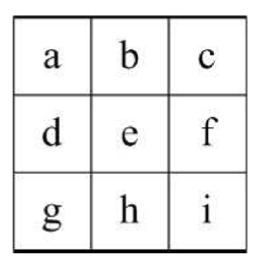
Figure 1. Schematic diagram of slope calculation. A certain pixel “e” is usually combined with eight adjacent pixels to form a slope, a~i stands for the elevation of each pixel.
Remotesensing 15 03184 g001
Figure 2. Slope of the whole Moon with a horizontal resolution of 512 pixels per degree (60 m at the equator) and a typical vertical accuracy of 3 to 4 m.
Remotesensing 15 03184 g002
Figure 3. The basic theory of sliding window algorithm. ① and ② represent the sliding window cyclic decision condition, ③ represents a single sliding window containing information and processing, ④ demonstrates the overlapping characteristics of sliding windows, ⑤ represents the completion of the sliding cycle of the original data.
Remotesensing 15 03184 g003
Figure 4. Spatial units based on the Queen proximity rule. “A” represents the spatial unit being studied, “B” represents the neighboring spatial unit for “A” under the Queen’s proximity rule, which contains the common vertex connection and common adjacent edge connection.
Remotesensing 15 03184 g004
Figure 5. The results of the evaluation of the whole Moon slope based on sliding windows combined with multiple indicators are shown in Figure (af) with a window size of 1° × 1° and in Figure (e) with a window size of 0.5° × 0.5°. (a) Results for the ratio of the whole Moon slope with a threshold of 20. (b) Results for the ratio of the whole Moon slope with a threshold of 8. (c) Results for the coefficient of variation of the whole Moon slope. (d) Results for the mean of the whole Moon slope. (e) Results for the whole Moon overall rating. (f) Results for the 0.5° × 0.5° whole Moon overall rating. Green snowflakes are expertly preselected landing sites, and red asterisks are available soft landing sites. Considering that the lower mean value reflects the overall flatness of the slope and the lower coefficient of variation reflects the dispersion of slope data, the color bars of results in Figure 5c,d were flipped (low value (blue) to high value (yellow) flip to high value (yellow) to low value (yellow) from top to bottom) to ensure consistency in the results and improve the overall presentation.
Remotesensing 15 03184 g005aRemotesensing 15 03184 g005b
Figure 6. K value clustering deviation map for different K values with different window sizes. The red circles represent the within-cluster sum of squares at the corresponding K values. (a) 1° × 1° window size. (b) 0.5° × 0.5° window size.
Remotesensing 15 03184 g006
Figure 7. Comparison of the whole Moon evaluation results of the sliding window and grid methods. (a) The whole Moon evaluation results of the grid algorithm are presented in the form of surface elements. (b) Whole Moon evaluation results of the sliding window algorithm in the form of surface elements. The black box represents the area selected for local comparison. For example, some areas with more landing points were selected to compare the differences between the grid and sliding window methods. The red asterisk represents the soft landing sites.
Remotesensing 15 03184 g007aRemotesensing 15 03184 g007b
Figure 8. WAC image maps of five local candidate regions (left column), grid method results (middle column), and sliding window method results (right column). The red asterisks are soft landing sites. (a) Sinus Iridum and Jura Mountains in northwestern Mare Imbrium. (b) Mare Vaporum and vicinity. (c) Mare Crisium and vicinity. (d) Tycho and vicinity. (e) Von Kármán impact crater and vicinity. According to the clustering results, the blue areas ranging from 0.81 to 1 represent suitable landing areas, and the green and red areas represent the quantitative results of less suitable and unsuitable landings, respectively.
Remotesensing 15 03184 g008aRemotesensing 15 03184 g008b
Figure 9. WAC images of the four candidate landing sites and the combined index results at different window sizes: first column (WAC images), second column (evaluation results at 1° × 1° window size), third column (evaluation results at 0.5° × 0.5° window size), and fourth column (evaluation results at 0.03125° × 0.03125° window size). (a) Candidate landing site, Aristarchus Crater. (b) Marius Hills. (c) Moscoviense Basin. (d) Orientale Basin.
Remotesensing 15 03184 g009aRemotesensing 15 03184 g009b
Table 1. The one-to-nine scale of parameters’ significance [63].
Strength of SignificanceExplanation
1Equal significance
3Medium significance
5Strong significance
7Very strong significance
9Maximum significance
2, 4, 6, 8Interim number between two adjacent numbers
Table 2. Weight proportion scale.
FactorMean SlopeThreshold Ratio (8)Threshold Ratio (20)Coefficient of VariationMoran’s INormalized Principal Eigenvector
Mean slope1153736.32%
Threshold ratio (8)1153736.32%
Threshold ratio (20)1/51/511/337.67%
Coefficient of variation1/51/531715.78%
Moran’s I1/71/71/31/513.91%
Total 100.00%
Table 3. Ratio indices (RI) for various n scores [66].
n123456
RI000.580.901.121.24
Table 4. Quantification of soft landing sites’ slope scores. The average slope and threshold ratio reflect the general level of the window data and show whether the base condition for measuring the suitability for landing. The Moran index reflects the degree of spatial autocorrelation of the window data, reflecting the degree of aggregation of similar values and whether there is a sufficient concentrated area to accommodate landing. The coefficient of variation reflects the degree of dispersion of the window data and whether there are high outliers to influence landing.
No.DetectorAverageThreshold Ratio (8) *Cv *Moran’s IThreshold Ratio (20) *Overall Rating (1) *Overall Rating (0.5) *
1Luna92.820.880.370.970.980.900.82
1.660.950.230.960.990.940.77
4.990.770.540.970.980.830.86
2.720.910.310.950.990.920.81
2Luna130.460.990.050.8210.980.97
0.420.990.040.8210.980.97
0.550.990.080.9310.980.98
0.640.990.080.9310.980.98
3Luna160.8610.030.7810.990.96
0.8810.060.8610.990.96
0.9710.030.8410.990.97
110.040.8310.990.97
4Luna170.570.990.080.8910.980.98
0.660.990.100.9110.980.98
0.5310.050.8210.990.98
0.090.990.090.8910.980.98
5Luna207.720.610.790.950.980.730.24
7.060.680.680.9510.980.770.32
8.190.570.870.950.970.340.76
7.500.650.730.960.950.750.75
6Luna212.330.950.230.9510.940.98
2.770.880.360.980.980.900.89
4.280.870.390.950.990.890.98
5.970.710.640.960.980.790.83
7Luna232.380.940.250.980.970.940.97
1.450.990.100.8910.980.98
1.320.990.110.8910.970.96
1.550.990.110.8910.970.98
8Luna241.320.990.110.8910.970.98
1.550.990.110.8910.970.98
1.080.990.080.8810.980.98
1.400.990.090.8910.980.97
9Surveyor11.390.960.200.9510.950.98
1.560.960.190.9410.950.98
0.6210.050.8210.990.98
1.160.990.110.9210.980.98
10Surveyor35.420.790.520.930.990.840.76
5.90.750.580.930.990.810.74
7.100.650.740.950.980.750.80
5.800.750.570.940.990.820.82
11Surveyor50.950.990.080.8510.980.98
0.8810.070.8610.980.97
0.960.990.090.8410.980.99
0.800.990.070.8610.980.98
12Surveyor60.950.990.080.8510.980.88
0.8810.070.8610.980.82
0.960.990.090.8410.980.93
0.800.990.070.8610.980.82
13Surveyor75.700.780.530.920.990.830.83
5.260.820.470.911.00.860.88
5.820.770.550.9310.830.87
7.010.650.730.960.980.750.93
14Apollo111.470.980.150.9310.970.96
1.220.980.130.9210.970.96
1.430.980.140.9210.970.97
1.170.990.100.8910.980.98
15Apollo120.760.990.080.8910.980.97
0.750.990.090.8910.980.97
0.850.990.100.8910.980.97
0.780.990.090.8810.980.96
16Apollo143.300.950.230.8710.940.95
3.280.950.230.8710.940.94
3.380.950.230.8710.940.95
3.940.900.340.9310.910.95
17Apollo156.150.730.600.9210.800.82
5.640.770.550.9410.830.79
6.20.730.600.950.990.800.84
5.990.740.590.950.990.810.85
18Apollo164.250.860.410.9110.880.87
5.240.820.480.920.990.850.87
4.440.820.460.930.990.860.86
5.340.800.500.9210.850.82
19Apollo179.630.530.940.980.840.300.31
11.080.451.110.980.800.250.74
8.460.580.850.980.890.340.25
9.320.501.010.970.910.290.33
20CE-30.830.990.110.9410.980.98
0.6110.050.8110.980.98
0.900.980.120.9310.970.98
0.7810.070.8310.980.98
21CE-41.250.990.070.8510.980.99
1.010.990.070.8410.980.99
0.9510.060.8310.980.98
0.9210.070.8310.980.98
22CE-50.950.970.170.9710.960.98
0.5210.040.8010.990.98
0.5710.060.8310.980.99
0.6710.050.8510.990.99
* The value in the brackets of the threshold ratio column identifies the threshold value. Cv represents the coefficient of variation. The value in the brackets of the overall rating column identifies the window size, with 1 representing 1° × 1° and 0.5 representing 0.5° × 0.5°. The red font in the table represents windows that are not suitable for landing.
Table 5. Statistics of suitable landing indicators for candidate landing regions.
No.Candidate Landing SiteWindow SizeNumber of Suitable WindowsTotal Number of WindowsArea of Candidate Landing Zones (km2)Percentage of Suitable Landing Area
1Aristarchus Crater1° × 1°4074411000.92
0.5° × 0.5°182219350.94
0.03125° × 0.03125°369,306408,3210.90
2Marius Hills1° × 1°4374411000.99
0.5° × 0.5°165316810.98
0.03125° × 0.03125°396,861408,3210.97
3Moscoviense Basin1° × 1°60536609000.17
0.5° × 0.5°389915,1250.26
0.03125° × 0.03125°1,806,6873,682,5610.49
4Orientale Basin1° × 1°1713808020000.21
0.5° × 0.5°1219033,0890.37
0.03125° × 0.03125°4,518,4418,186,2410.55
Disclaimer/Publisher’s Note: The statements, opinions and data contained in all publications are solely those of the individual author(s) and contributor(s) and not of MDPI and/or the editor(s). MDPI and/or the editor(s) disclaim responsibility for any injury to people or property resulting from any ideas, methods, instructions or products referred to in the content.